Dissipation in gases trapped in time–dependent external potentials

Abstract

We investigate an ideal gas in a time–dependent external trapping potential. We use the Boltzmann equation with the relaxation time ansatz to explore the time–dependent energy of an adiabatically isolated system. In particular we are interested on the dissipation during a potential change along a given protocol with finite velocity. The role of the relaxation less evolution as a limiting case is studied: starting from an equilibrium distribution and for small times the energy of the gas with relaxation is always smaller than that of the relaxation–less. This means that relaxation processes show an ambivalent behavior: on the one hand entropy production, but on the other hand reduction of dissipation by driving back the system into equilibrium.

I Introduction

Dissipation of energy in gases or liquids due to a moving body is at the core of physical theories such as hydrodynamics, statistical physics or kinetic theory. Some interesting new results at a fundamental level, regarding the connection of equilibrium and non–equilibrium free energy differences, as the Jarzynski equation, or the relation between dissipation and the asymmetry of time–reversal processes are knownJarzynski (1996); Crooks (1999); Seifert (2005); Kawai et al. (2007); Parrondo et al. (2009). These results have been extended from classical to quantum mechanical systems Mukamel (2003); Engel and Nolte (2007); Andrieux and Gaspard (2008). In this work we investigate the dissipation process in gases using the Boltzmann equation (BE) with a time–dependent external potential. The main motivation for considering this problem was the ambivalent behavior of elastic collisions during the potential deformation: on the one hand collisions do not change the energy of the colliding particles, and this is also true for a time–dependent potential, since the collisions are described as pointlike in phase space. On the other hand it is immediately clear that the energy of the gas in a time–dependent potential must depend on the collisions during the potential change. It makes a difference in the distribution function if in the BE collisions are present or not. The first impulse to investigate such problems using kinetic theory was the study of Bose–Einstein condensation in trapped gases, where one can reach the condensation of a Bose gas by changing the trapping potential Stamper-Kurn et al. (1998); Dalvovo et al. (1999).
The paper is organized as follows: Sec.  II gives a short overview of the theoretical elements and formulas used to derive the main results represented in Sec.  III. Sec. IV gives a numerical example and Sec. V conclusion and outlook. The appendix contains a proof of the H–Theorem for time–dependent potentials and the relaxation time ansatz in the BE.

II General approach: kinetic theory

First we present some general equations of kinetic theory used in this paper. The central quantity to describe the system is the time–dependent one particle distribution function $f({\textbf{p}},{\textbf{x}},t)$. The distribution function depends on the one particle phase space coordinates $\{{\textbf{p}},{\textbf{x}}\}$ (momentum and space coordinates, sometimes suppressed to simplify notation) and time $t$ (also suppressed sometimes). $f$ is normalized to the number of particles $N$,

$$\int f({\textbf{p}},{\textbf{x}},t)\mathrm{d}\Gamma=N~{}.$$ (1)

Here $\mathrm{d}\Gamma=\mathrm{d}^{3}x\mathrm{d}^{3}p/(2\pi)^{3}$ denotes the volume element in the 6 dimensional phase space (we omit always Planck’s constant $\hbar$ and the Boltzmann constant $k_{B}$).

II.1 Kinetic equation

We consider a gas in a time–dependent external potential $U({\textbf{x}},t)$. The time evolution of the distribution function is given by the Boltzmann equation (see for example Lifschitz and Pitajewski (1982))

$$\frac{\partial f}{\partial t}+\frac{{\textbf{p}}}{m}\cdot\nabla_{\textbf{x}}f-\nabla_{\textbf{x}}U({\textbf{x}},t)\cdot\nabla_{\textbf{p}}f=\left(\frac{\partial f}{\partial t}\right)_{coll}~{}.$$ (2)

Here $(\partial f/\partial t)_{coll}$ denotes the collision integral, which we approximate by the relaxation time ansatz,

$$\left(\frac{\partial f}{\partial t}\right)_{coll}=-\frac{f-f_{g}}{\tau}~{}.$$ (3)

Because the external potential is time–dependent the equilibrium distribution $f_{g}({\textbf{p}},{\textbf{x}},t)$ becomes time–dependent as well,

$$f_{g}({\textbf{p}},{\textbf{x}},t)=\exp\{-\beta(t)[H({\textbf{p}},{\textbf{x}},t)-\mu(t)]\}~{}.$$ (4)

Here $\mu(t)$ is the time–dependent chemical potential, $\beta(t)=1/T(t)$ corresponds to the time–dependent inverse temperature $T(t)$ and

$$H({\textbf{p}},{\textbf{x}},t)=\frac{{\textbf{p}}^{2}}{2m}+U({\textbf{x}},t)~{},$$ (5)

is the one particle Hamiltonian for particles with mass $m$ and without inner degrees of freedom. The equilibrium distribution Eq. (4) does not contain a macroscopic momentum or angular momentum because we restrict ourselves to spherical symmetric potentials to make the discussion transparent. The main result Eq. (16) is not affected by this restriction, as the derivations show, since the explicit structure of $f_{g}$ does not enter. So let us assume that the number of particles and the energy for a fixed time are the only conserved quantities, which allow the determination of $\beta(t)$ and $\mu(t)$ in Eq. (4). In particular we have the relation

$$\int f_{g}({\textbf{p}},{\textbf{x}},t)\mathrm{d}\Gamma=\int f({\textbf{p}},{\textbf{x}},t)\mathrm{d}\Gamma~{},$$ (6)

ensuring conservation of the number of particles. The conservation of energy $E(t)$ for a fixed time is expressed as

$$E(t)=\int H({\textbf{p}},{\textbf{x}},t)f_{g}({\textbf{p}},{\textbf{x}},t)\mathrm{d}\Gamma={}$$

$$\int H({\textbf{p}},{\textbf{x}},t)f({\textbf{p}},{\textbf{x}},t)\mathrm{d}\Gamma~{}.$$ (7)

Eq. (2) with an initial condition (in our case a Maxwell–Boltzmann distribution) and the two conditions Eq. (6) and Eq. (II.1) are the basis for our analytical and numerical studies in Sec. IV. We remark that Eq. (2) due to Eq. (6) and Eq. (II.1) becomes non linear, in contrast to the Focker–Planck equation, which is a linear evolution equation.

II.2 Entropy

A central quantity is the nonequilibrium entropy of the gas. For a given one particle distribution function it is computed as Lifschitz and Pitajewski (1982)

$$S(t)=-\int f({\textbf{p}},{\textbf{x}},t)\ln[f({\textbf{p}},{\textbf{x}},t)]\mathrm{d}\Gamma~{}.$$ (8)

One can proof the validity of the H–Theorem, $\dot{S}(t)=-\int\ln(f)(\partial f/\partial t)_{coll}\mathrm{d}\Gamma\geq 0$ with the relaxation time ansatz and a time–dependent external potential also. For details see the appendix App. A. Here we need an additional expression for $S(t)$ for gases not far from equilibrium. We split the distribution function as $f=f_{g}+\delta f_{g}$, where $\delta f_{g}$ denotes the small deviation of $f$ from the equilibrium. Expansion of the logarithm in Eq. (8) up to second order and some lines of algebraic simplifications yields

$$S(t)=S_{eq}(t)-\int\frac{\delta f_{g}^{2}}{2f_{g}}\mathrm{d}\Gamma~{}.$$ (9)

Here $S_{eq}(t)=\beta(t)E(t)-\beta(t)\mu(t)N$ is the time–dependent equilibrium entropy, reached when $\delta f_{g}=0$ . Due to relaxation $\delta f_{g}(t)$ becomes smaller and smaller and at the end (for a fixed potential) $S(t\gg\tau)=S_{eq}$.

III Distribution function: Perturbation theory

To proceed we have to compute the distribution function. Because the analytical integration of the kinetic equation for time–dependent potentials (even with the simple relaxation time ansatz) in general is not possible we look for a perturbation theory approach. There are two interesting limiting cases as starting points for this attempt: an infinitely slow potential change, corresponding to the adiabatic time evolution of the distribution function, and the relaxation less time evolution [$\tau\rightarrow\infty$ in Eq. (2)], corresponding to the Liouville evolution (denoted as $f_{L}$), respectively. We choose here the second way, where the system has a large relaxation time, compared with the time $t$, for which we are interested, so that $t/\tau\ll 1$. An analytical integration of the time–dependent collision less BE is still impossible in general, but here we do not need the solution explicitly.

III.1 First order expression

The lowest (zeroth) order of such an expansion is the time–dependent Liouville function $f_{L}$. We split the true distribution function into two parts,

$$f=f_{L}+\delta f_{L}$$ (10)

where $f_{L}({\textbf{p}},{\textbf{x}},t)$ is the solution of the collision less BE and $\delta f_{L}$ is the deviation from the actual distribution. If we enter with this ansatz into Eq. (2), we get for the first order correction

$$\delta f^{(1)}_{L}({\textbf{p}},{\textbf{x}},t)=-\frac{1}{\tau}\int_{0}^{t}\mathrm{d}t^{\prime}[f_{L}({\textbf{p}},{\textbf{x}},t^{\prime})-f^{(0)}_{g}({\textbf{p}},{\textbf{x}},t^{\prime})]~{}.$$ (11)

This first order expression is sufficient as long as the ratio $t/\tau$ is small. The equilibrium distribution $f^{(0)}_{g}$ is computed using $f_{L}$ on the right hand side of the conditions Eq. (6), Eq. (II.1). We do not require the computation of $f_{g}^{(0)}$, but we know that it does not depend on the relaxation time $\tau$.

III.2 Energy

The distribution function Eq. (10) with Eq. (11) allows us to clarify the influence of $\tau$ on the dissipated energy. We consider the begin of a potential change, where the distribution function deviates weakly from equilibrium. The starting point is Eq. (9), where we replace $S(t)$, using Eq. (22), by

$$S(t)=S(0)+\frac{t}{\tau}\int\frac{\delta f_{g}^{2}}{2f_{g}^{(0)}}\mathrm{d}\Gamma~{}.$$ (12)

Now we use $f$ from Eq. (10), where we approximate the time integral in Eq. (11) by a trapezoidal rule. After some simplifications we obtain up to the order $(t/\tau)^{2}$,

$$S_{eq}(t)=S(0)+\left[1-\left(\frac{t}{\tau}\right)^{2}\right]\int\frac{(f_{L}-f_{g}^{(0)})^{2}}{2f_{g}^{(0)}}\mathrm{d}\Gamma~{}.$$ (13)

The dissipated energy (heat) is given by $T(t)[S_{eq}(t)-S(0)]$. For small times the choice $T(t)=T_{ad}(t)$ is reasonable and we get

$$E(t)=E_{ad}(t)+T_{ad}(t)\left[1-\left(\frac{t}{\tau}\right)^{2}\right]\int\frac{(f_{L}-f_{g}^{(0)})^{2}}{2f_{g}^{(0)}}\mathrm{d}\Gamma~{}.$$ (14)

For $\tau\rightarrow\infty$ we obtain from this expression

$$E_{L}(t):=\int Hf_{L}\mathrm{d}\Gamma=E_{ad}(t)+T_{ad}(t)\int\frac{(f_{L}-f_{g}^{(0)})^{2}}{2f_{g}^{(0)}}\mathrm{d}\Gamma~{}.$$ (15)

and further (for $t/\tau\ll 1$)

$$E(t)\leq E_{L}(t)~{}.$$ (16)

This result shows that the time–dependent energy $E_{L}$ represents an upper bound of the energy of the gas, independent of the characteristics of the potential. Relaxation favors minimization of dissipation. This is remarkable because the Liouville evolution itself conserves entropy $S(t)=-\int f_{L}\ln(f_{L})\mathrm{d}\Gamma=S(0)$. For larger times Eq. (16) can be violated, however for slow potential changes it must fulfilled, because the true distribution functions $f$ and $f_{g}$ approaches the adiabatic distribution function $f_{ad}$. Because the dissipated energy is given by $E_{diss}=E-E_{ad}$ one obtains $E_{diss}\leq E_{L}-E_{ad}$.

IV Numerical example

For a model potential we consider a one dimensional harmonic oscillator with time–dependent frequency, as widely used to investigate dissipation of Brownian particles and the Jarzynski equation Speck (2011); Engel and Nolte (2007). An increase/decrease of the frequency leads to a compression/expansion of the gas. We integrate numerically the BE with the relaxation time ansatz and monitor the energy (and entropy) of the gas during the potential change. The numerical method is based on a discretization of the phase space into equal sized cells and a numerical integration of the resulting ordinary differential equations. To obtain the time–dependent equilibrium distribution $f_{g}$, we compute for each time step the integrals Eq. (6) and Eq. (II.1) and solve numerically the resulting equations for $\beta$ and $\mu$ (where the values for the quasistatic potential change are used as a starting guess). This procedure runs well and there are no numerical problems which we should report. To be sure that energy conservation (not only number of particles) for a fixed potential is fulfilled, the used numerical limits of the phase space must be large enough. The external potential has the form

$$U(x,t)=\frac{1}{2}m\omega(t)^{2}x^{2}~{},\hskip 14.22636pt\omega(t)=\omega_{0}+\Delta\omega\sin(2\pi t/t_{f})~{}.$$ (17)

Here $t_{f}$ characterize the switching time and likewise denotes the final integration time. We set $t_{f}=1$ as our time scale. We choose $\omega_{0}t_{f}=1$ and $|\Delta\omega/\omega_{0}|=0.5$, so we are far away from adiabatic conditions. The mean free fly time of a particle is on the order $\sim 1/(\omega_{0}N)$, where we have choosen $N=1250$ (and the ratio initial temperature to initial frequency $T_{0}/\omega_{0}=200$). For Bose gases at low temperatures and densities as H and Na in magneto–optical traps the relaxation time differs dramatically due to the different $s$-wave scattering cross sections (by a factor of $\sim 10^{3}$)Walraven (1996). For an adiabatic potential change the temperature of the gas is given by $T_{ad}/T_{0}=\omega/\omega_{0}$ and the energy $E_{ad}/E_{0}=\omega/\omega_{0}$, respectively.

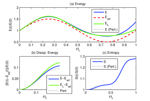
Figure 1: (color online) (a) Energy of the gas during the compression and expansion. The frequency ratio is $\Delta\omega/\omega_{0}=0.5$. The green line corresponds to the Liouville evolution ($E_{L}$) and the blue line to a evolution with finite relaxation time ($\tau/t_{f}=0.5$). The red dotted line is the adiabatic limit and in black–dotted it is shown the result from the perturbation theory. (b) shows the dissipated energy for a time regime where Eq. (14) is valid. In (c) we have plotted the entropy of the gas and the approximation according Eq. (12). For small times $E_{L}$ is the upper bound for the energy.

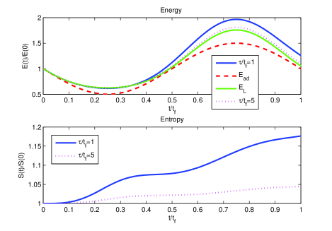
Figure 2: (color online) Energy of the gas during the expansion and compression cycle, $\Delta\omega/\omega_{0}=-0.5$. Although it is difficult to see the energy corresponding to the Liouville evolution $E_{L}$ for small times is always greater than all others, in accordance to Eq. (16).

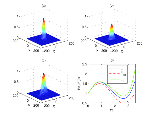
Figure 3: (color online) The same potential deformation as in Fig. 1 but 3.5 times slower as there (with $\tau=t_{f}$). In (a) it is shown the initial Maxwell–Boltzmann distribution in phase space [in units $(P,X)=(p/\sqrt{mT_{0}},x\sqrt{m\omega_{0}^{2}/T_{0}})$], (b) shows the partially relaxed distribution at $t=t_{f}$ and (c) shows the Liouville distribution $f_{L}(t_{f})$. In (d) we have plotted again the energy of the gas (blue line) to demonstrate the validity of Eq. (16) for the entire time.

In Fig. 1 we show the energy/entropy for one compression – expansion chicle as a function of time for a gas with specified relaxation time. The lines for the energy reflect the time–dependent frequency, whereas the entropy increase as required from the H–theorem. We have also plotted the perturbation theory expressions Eq. (14) and Eq. (12) to demonstrate the result Eq. (16). Fig. 2 demonstrates the same behavior of the gas for the opposite chicle, where first the frequency $\omega$ decrease and hereafter increase (expansion and compression). Here we have plotted the time–dependent energy of two gases with different relaxation times and additional $E_{ad}(t)$ and $E_{L}(t)$. For small times $E_{L}(t)$ is an upper bound of the energy. Fig. 3 shows the distribution function, obtained by the numerical integration. The initial Maxwell–Boltzmanm distribution (a) and the collision less evolved function (c), as well as an example with finite relaxation time (b) the are plotted. In this case (slower potential change as in the previous example) the energy of the $\tau\neq 0$ system is smaller as $E_{L}$ for the entire switching time.

V Conclusion and outlook

In this paper we have discussed energy dissipation in gases in time–dependent trapping potentials. Using the Boltzmann equation with the relaxation time ansatz we have shown that the dissipated energy depends on the relaxation time. In particular we have demonstrated using perturbation theory, that for small times (compared with the relaxation time) the relaxation less time evolution always leads to a higher energy than that with finite relaxation time. On this time scales relaxation decreases dissipation. The derivation shows that this statement is fairly general: it does not depend on the shape of the external potential. It would be interesting to make some numerical studies with the full collision integral of the BE to check if the results of this paper are still valid Markowich et al. (2004); Goulko et al. (2012).

Appendix A H–Theorem for time–dependent potentials and the relaxation time ansatz

The time derivative of the entropy in the relaxation time ansatz is equal

$$\dot{S}(t)=\int\ln(f)\frac{f-f_{g}}{\tau}\mathrm{d}\Gamma~{}.$$ (18)

If we set inside the logarithm $f=f_{g}+\delta f_{g}$ we obtain

$$\int\ln(f)\frac{f-f_{g}}{\tau}\mathrm{d}\Gamma=\frac{1}{\tau}\int f\ln(f)\mathrm{d}\Gamma-{}$$

$$\frac{1}{\tau}\int f_{g}\ln\left[f_{g}\left(1+\frac{\delta f_{g}}{f_{g}}\right)\right]\mathrm{d}\Gamma~{}.$$ (19)

Now we split the argument of the logarithm in to two parts,

$$\dot{S}(t)=\frac{S_{eq}(t)-S(t)}{\tau}-\frac{1}{\tau}\int f_{g}\ln\left[1+\frac{\delta f_{g}}{f_{g}}\right]\mathrm{d}\Gamma~{},$$ (20)

where we have defined the equilibrium entropy $S_{eq}(t)=-\int f_{g}\ln(f_{g})\mathrm{d}\Gamma$. Because $f_{g}$ is the equilibrium distribution, corresponding to the same number of particles and energy as $f$, it follows $S_{eq}(t)-S(t)\geq 0$. The last integral in Eq. (20) is positive for all $t$. If $x>0$ is a real number, then $\ln(x)\leq x-1$ is always true. Using this for the integral above we obtain ($f_{g}\geq 0$),

$$\int f_{g}\ln\left[1+\frac{\delta f_{g}}{f_{g}}\right]\mathrm{d}\Gamma\leq\int\delta f_{g}\mathrm{d}\Gamma=0~{}.$$ (21)

With the $-$ sign in front of the integral in Eq. (20) we conclude that $\dot{S}\geq 0$.
In the text we use an expression for $\dot{S}$ for small $\delta f_{g}$. One can obtain this expression by insertion of $f=f_{g}+\delta f_{g}$ into the logarithm in Eq. (18) and a series expansion,

$$\dot{S}(t)\approx\frac{1}{\tau}\int\frac{\delta f_{g}^{2}}{f_{g}}\mathrm{d}\Gamma~{}.$$ (22)

References

- Jarzynski (1996) C. Jarzynski, Phys. Rev. Lett. 78, 14 (1996).
- Crooks (1999) G. E. Crooks, Phys. Rev. E 60, 3 (1999).
- Seifert (2005) U. Seifert, Phys. Rev. Lett. 95, 040602 (2005).
- Kawai et al. (2007) R. Kawai, J. M. R. Parrondo, and C. V. den Broeck, Phys. Rev. Lett. 98, 080602 (2007).
- Parrondo et al. (2009) J. Parrondo, C. van den Broeck, and R. Kawai, New Journal of Phys. 11, 073008 (2009).
- Engel and Nolte (2007) A. Engel and R. Nolte, EPL 79, 10003 (2007).
- Mukamel (2003) S. Mukamel, Phys. Rev. Lett. 90, 17 (2003).
- Andrieux and Gaspard (2008) D. Andrieux and P. Gaspard, Phys. Rev. Lett. 100, 230404 (2008).
- Dalvovo et al. (1999) F. Dalvovo, S. Giorgini, L. P. Pitaevskii, and S. Stringari, Rev. Mod. Phys. 71, 463–512 (1999).
- Stamper-Kurn et al. (1998) D. Stamper-Kurn, H. Miesner, A. Chikkatur, S. Inouyec, J. Stenger, and W. Ketterle, Phys. Rev. Lett. 81, 2194–2197 (1998).
- Lifschitz and Pitajewski (1982) E. M. Lifschitz and L. P. Pitajewski, Lehrbuch der Theoretischen Physik X (Akademie Verlag Berlin, 1982).
- Speck (2011) T. Speck, J. Phys. A: Math. Gen. 44, 305001 (2011).
- Walraven (1996) J. T. M. Walraven, Quantum dynamics of simple systems (SUSSP Proceedings 44, 1996).
- Goulko et al. (2012) O. Goulko, F. Chevy, and C. Lobo, New Journal of Phys. 141, 073036 (2012).
- Markowich et al. (2004) P. Markowich, L. Pareschi, and W. Bao, Quantum kinetic theory: modelling and numerics for Bose-Einstein condensation (Birkhauser, 2004).