Automated construction of maximally localized Wannier functions: Optimized projection functions method

Abstract

Maximally localized Wannier functions are widely used in electronic structure theory for analyses of bonding, electric polarization, orbital magnetization, and for interpolation. The state of the art method for their construction is based on the method of Marzari and Vanderbilt. One of the practical difficulties of this method is guessing functions (initial projections) that approximate the final Wannier functions. Here we present an approach based on optimized projection functions that can construct maximally localized Wannier functions without a guess. We describe and demonstrate this approach on several realistic examples.

I Introduction and motivation

Within the quasiparticle approximation, the electronic states of a crystal can be described in terms of single-particle Bloch functions $\psi_{n\mathbf{k}}(\mathbf{r})$. These functions are eigenstates of the crystal Hamiltonian, and can be labeled by their band index $n$ and crystal momentum $\mathbf{k}$. Wannier functions (WFs) provide an alternative representation in which an entire band of electrons is described by a single function $\ket{\mathbf{R}n}$ localized in or near the unit cell labeled by the lattice vector $\mathbf{R}$. In their simplest form, WFs are obtained from the Bloch functions via the Fourier transformation

$$\ket{\mathbf{R}n}=\frac{V}{{(2\pi)}^{3}}\int_{\textrm{BZ}}\textrm{d}\mathbf{k}\,e^{-i\mathbf{k}\cdot\mathbf{R}}\ket{\psi_{n\mathbf{k}}},$$ (1)

where $V$ is the volume of the real-space primitive cell. The definition of WFs is not unique because there is a gauge freedom in the right-hand side of Eq. (1). Namely, at each $\mathbf{k}$ point and for each $n$, one can change the overall phase of the Bloch state $\ket{\psi_{n\mathbf{k}}}$. In fact, one often considers an even more general gauge choice which allows an arbitrary unitary transformation of a set of $N$ bands at each $\mathbf{k}$ point,

$$\ket{\psi_{n\mathbf{k}}}\rightarrow\sum_{m}u^{(\mathbf{k})}_{mn}\ket{\psi_{m\mathbf{k}}}.$$ (2)

We focus here on the case when these $N$ bands are isolated from the rest. The choice of gauge is now expressed through a $\mathbf{k}$-dependent $N\!\times\!N$ unitary matrix $u^{(\mathbf{k})}$.

When Wannier functions are localized in real space they have a wide use in the electronic structure community. An extensive review of maximally localized Wannier functions (MLWFs) and their properties and applications can be found in Ref. 1. For example, they have been used in the description of electronic polarizationWu et al. (2006) and orbital magnetization, in addition to being used for interpolation of band structures and matrix elements Yates et al. (2007); Giustino et al. (2007); Noffsinger et al. (2010) and electron transport calculations.Pizzi et al. (2014)

For this reason, one often uses the gauge freedom $u^{(\mathbf{k})}$ so that the corresponding WFs are localized. As a general consequence of the Fourier transform, the localization of the WFs $\ket{\mathbf{R}n}$ in $\mathbf{r}$ space will depend on the smoothness of the gauge $u^{(\mathbf{k})}$ in $\mathbf{k}$ space. If the $\psi_{n\mathbf{k}}(\mathbf{r})$ are chosen with random overall complex phases [which often happens if $\psi_{n\mathbf{k}}(\mathbf{r})$ are acquired numerically by diagonalizing a $\mathbf{k}$-dependent Hamiltonian matrix separately for each $\mathbf{k}$ point] the WFs obtained from Eq. (1) need not be localized. However, if matrices $u^{(\mathbf{k})}$ are chosen so that Bloch states are smooth in $\mathbf{k}$ space (smooth gauge), the corresponding WFs will be localized in $\mathbf{r}$ space.

The idea of maximally localized Wannier functions and a procedure for obtaining them from a set of composite bands was introduced by Marzari and VanderbiltMarzari and Vanderbilt (1997) for isolated bands and later extended to the case of entangled bands.Souza et al. (2001) Maximally localized Wannier functions are constructed by choosing a gauge $u^{(\mathbf{k})}_{mn}$ for Eq. (2) that minimizes the spread functional

$$\Omega =\sum_{n}\quantity[\expectationvalue{r^{2}}_{n}-\overline{\mathbf{r}}_{n}^{2}],$$ (3)

where

$$\expectationvalue{r^{2}}_{n} =\expectationvalue{r^{2}}{\mathbf{0}n},$$ (4)

$$\overline{\mathbf{r}}_{n} =\expectationvalue{\mathbf{r}}{\mathbf{0}n}.$$ (5)

Here the spread functional $\Omega$ is written in terms of the Wannier functions $\ket{\mathbf{0}n}$. Usually there exists a global minimum of $\Omega$ corresponding to a unique choice of $u^{(\mathbf{k})}$ (up to translation of the WFs and their overall complex phase), but in some cases there are multiple solutions.Marzari and Vanderbilt (1997)

Using the general form of Eq. (1) including the $u^{(\mathbf{k})}$ matrix in Eq. (2), the spread can be recast in terms of the Bloch states. More specifically, $\Omega$ can be expressed only as a function of the overlaps of the periodic parts of the Bloch functions at neighboring $\mathbf{k}$ points $\mathbf{k}$ and $\mathbf{k}+\mathbf{b}$,

$$m^{(\mathbf{k},\mathbf{b})}_{ij}=\innerproduct{u_{i\mathbf{k}}}{u_{j\mathbf{k}+\mathbf{b}}}.$$ (6)

See Appendix A for an explicit definition of $\Omega$ in terms of $m^{(\mathbf{k},\mathbf{b})}$,

$$\Omega=\Omega\quantity[m^{(\mathbf{k},\mathbf{b})}].$$ (7)

Here we only note that spread $\Omega$ can be decomposed into three parts: the invariant part, which does not depend on the gauge, and the diagonal part and the off-diagonal parts which do,

$$\Omega\quantity[m^{(\mathbf{k},\mathbf{b})}]=\Omega_{\text{I}}+\Omega_{\text{D}}+\Omega_{\text{OD}}.$$ (8)

The procedure for minimizing $\Omega$, outlined in Refs. 7 and 8, is implemented in the Wannier90 codeMostofi et al. (2008) and has become the standard method for obtaining localized WFs. A notable drawback in the standard approach that we address in this manuscript is that one often needs to provide a good initial guess of the MLWFs to find the global minimum of $\Omega$. In this work we demonstrate a modified procedure, in which localized Wannier functions are constructed as a linear combination of physically based atom-centered orbitals without requiring an initial guess, as in the standard approach.Marzari and Vanderbilt (1997) This is achieved by finding optimal projection functions (OPFs) so that the resulting Wannier functions obtained via projection (as in Sec. II.1) are as localized as possible. This OPF method could, for example, be used in constructing material properties databases, such as the database of the Materials Project,Jain et al. (2013) by providing a simple localized Hamiltonian that could serve as a descriptor for the electronic structure of a material. We present the theoretical approach and numerical methods in Sec. II and III. Several realistic materials are investigated in Secs. IV to illustrate our approach for constructing localized WFs.

Schemes beyond the standard implementationMarzari and Vanderbilt (1997); Souza et al. (2001); Mostofi et al. (2008) have been developed by others to improve the construction of MLWFs and their properties. The inclusion of unoccupied anti-bonding states has been shownThygesen et al. (2005a); *PhysRevB.72.125119 to give more localized Wannier functions, but at the expense of a chemical picture of the occupied states. Additionally, constraints on the $u^{(\mathbf{k})}$ matrices can be imposed in order to construct localized Wannier functions that possess all the space group symmetries of the crystal.Sakuma (2013)

II Standard approach

Here we summarize the main result of Ref. Marzari and Vanderbilt, 1997 for a two-step construction of maximally localized Wannier functions. In the first step of minimizing the spread functional $\Omega$ one needs to guess orbitals $g_{j}(\mathbf{r})$ with roughly the same orbital characters and real-space location $\overline{\mathbf{r}}_{j}$ as the target MLWFs. This choice is often done based on an intuitive understanding of the band structure of the crystal under investigation. Given a choice of $g_{j}(\mathbf{r})$ close to target WFs, one constructs the gauge for which spread functional $\Omega$ is near its global minimum (better choices give $\Omega$ closer to the global minimum). In the second step, this initial gauge choice is iteratively optimized until $\Omega$ reaches a global minimum. In practice, the second step usually reduces the spread $\Omega$ only by 20% or less.

II.1 First step

Now we describe the first step of this procedure in the simple case of a single band of states $\psi_{\mathbf{k}}(\mathbf{r})$. Given a localized function $g(\mathbf{r})$ approximating the target MLWF at the origin, we first project it onto the Bloch state $\psi_{\mathbf{k}}(\mathbf{r})$ at each $\mathbf{k}$

$$a^{(\mathbf{k})}=\innerproduct{\psi_{\mathbf{k}}}{g}.$$ (9)

Now we rotate the phase of Bloch state $\psi_{\mathbf{k}}(\mathbf{r})$ so that the relative phase of rotated Bloch state and $g(\mathbf{r})$ is zero for all $\mathbf{k}$ points,

$$\ket{\psi_{\mathbf{k}}}\rightarrow a^{(\mathbf{k})}\quantity(a^{(\mathbf{k})*}a^{(\mathbf{k})})^{-1/2}\ket{\psi_{\mathbf{k}}}.$$ (10)

It is easy to check that if the initial guess $g(\mathbf{r})$ were a true target MLWF, inserting these rotated Bloch states into Eq. (1) would give back the target MLWF. However, since $g(\mathbf{r})$ is only an approximation, the spread $\Omega$ of the rotated Bloch states is not exactly at the global minimum. For a good guess $g(\mathbf{r})$, however, the spread should be close to the global minimum.

Following the procedure in the case of a single band, we now generalize it to the case of $N$ composite bands. First, we choose a set of $N$ localized orbitals $g_{j}(\mathbf{r})$ that are approximately equal to the $N$ target MLWFs,

$$\ket{g_{j}}\approx\ket{\mathbf{0}j}.$$ (11)

Here we choose for convenience $\ket{g_{j}}$ to be close to the MLWFs near the origin ($\mathbf{R}=\mathbf{0}$), but in principle any other $\mathbf{R}$ can be chosen.

Next we compute the overlap between all $N$ Bloch bands and $N$ initial guesses for the WFs,

$$a^{(\mathbf{k})}_{ij}=\innerproduct{\psi_{i\mathbf{k}}}{g_{j}}.$$ (12)

Unlike the case of a single band, $a^{(\mathbf{k})}$ for an isolated group of N Bloch bands is a $N\!\times\!N$ matrix, so that Eq. (10) generalizes to

$$\ket{\psi_{i\mathbf{k}}}\rightarrow\sum_{j}u^{(\mathbf{k})}_{ji}\ket{\psi_{j\mathbf{k}}}=\sum_{jl}a_{jl}\quantity[\quantity(a^{\dagger}a)^{-1/2}]_{li}\ket{\psi_{j\mathbf{k}}}.$$ (13)

Here, to simplify notation, we suppress the $\mathbf{k}$ dependence of $a$. The inverse square root on the right-hand side is the matrix square root of $\quantity(a^{\dagger}a)^{-1}$. For further simplification, define $u_{x}$, for an arbitrary matrix $x$, as

$$u_{x}\equiv x(x^{\dagger}x)^{-1/2}.$$ (14)

The matrix $u_{x}$ is unitary by construction. In fact, it is the closest unitary approximation of $x$.

In practice, the unitary matrix $u_{x}$ is obtained via the singular value decomposition (SVD) of $x$. If $x=zdv$ is a SVD with $z$ and $v$ unitary, and $d$ diagonal, then $u_{x}$ is simply $zv$. Given this notation, the earlier gauge transformation from Eq. (13) now reads

$$\ket{\psi_{i\mathbf{k}}}\rightarrow\sum_{j}\quantity[u^{(\mathbf{k})}_{a}]_{ji}\ket{\psi_{j\mathbf{k}}}.$$ (15)

As in the case of a single band, if trial orbitals $g_{j}(\mathbf{r})$ were chosen close enough to the target MLWF, the gauge $u^{(\mathbf{k})}_{a}$ from Eq. (15) will by definition give a spread close to the global minimum,

$$\Omega=\Omega\quantity[u^{(\mathbf{k})\dagger}_{a}m^{(\mathbf{k},\mathbf{b})}u^{(\mathbf{k}+\mathbf{b})}_{a}].$$ (16)

Here we implicitly wrote $\Omega$ in terms of overlap matrices $m^{(\mathbf{k},\mathbf{b})}$ and used gauge transformation of Bloch states from Eq. (2) to get transformation of the overlap matrix $m^{(\mathbf{k},\mathbf{b})}$ defined in Eq. (6).

II.2 Second step

The initial gauge $u^{(\mathbf{k})}_{a}$ can be further improved in the second step by rotating, at each $\mathbf{k}$ point, the gauge from $u^{(\mathbf{k})}_{a}$ to $u^{(\mathbf{k})}_{a}v^{(\mathbf{k})}$ with an appropriate choice of $\mathbf{k}$-dependent matrices $v^{(\mathbf{k})}$. The spread functional $\Omega$ is minimized using the method of steepest descent. The gradient is determined by calculating the derivative of the spread with respect to the unitary matrices $v^{(\mathbf{k})}$ and then following the path along the direction which minimizes $\Omega$. Written more formally, the second step of the standard procedure finds a set of unitary $N\!\times\!N$ matrices

$$v^{(\mathbf{k})}\in\mathcal{U}(N,N),\text{ one for each $\mathbf{k}$,}$$ (17)

that

$$\text{minimize}\quad\Omega\quantity[v^{(\mathbf{k})\dagger}u^{(\mathbf{k})\dagger}_{a}m^{(\mathbf{k},\mathbf{b})}u^{(\mathbf{k}+\mathbf{b})}_{a}v^{(\mathbf{k}+\mathbf{b})}].$$ (18)

Quite generally, the global minimization of a function using the steepest descent algorithm is bound to work well when one starts near the global minimum. Otherwise it is quite possible for the algorithm to get stuck in a local minimum. In other words, the second step of the procedure will arrive at the true MLWFs as long as the initial guesses $g_{j}(\mathbf{r})$ in the first step are close enough. It is this issue that we aim to address in this manuscript: how to automatically construct a gauge that is guaranteed to be close to the global minimum.

III Alternative approach

In our approach, instead of choosing $N$ functions $g_{j}(\mathbf{r})$ that are close to the $N$ target MLWFs, we start with a larger set of $M$ functions ($M\!\geq\!N$) labeled $h_{j}(\mathbf{r})$. These functions $h_{j}$ will be chosen so that any MLWF near the origin ($\mathbf{R}=\mathbf{0}$) can approximately be written as a linear combination of $h_{j}$. In other words, the space spanned by $h_{j}$ must approximately contain, as a subset, the space spanned by the MLWFs near the origin,

$$\textrm{Span}\quantity(\ket{h_{j}})\supseteq\textrm{Span}\quantity(\ket{\mathbf{0}n}).$$ (19)

The requirement on $\ket{h_{j}}$ is significantly less restrictive than that on $\ket{g_{j}}$ in the standard approach. In fact, the requirement Eq. (19) should be rather easily satisfied. Since we expect MLWFs to be linear combinations of atomiclike valence electrons, we can simply choose $h_{j}$ to be a set of atom-centered atomic orbitals for each atom in the crystal basis and for each relevant atomiclike orbital in the valence (some combination of $s$, $p$, $d$, $f$ atomic orbitals, depending on the valence). If nominal valence atomiclike orbitals are not enough to satisfy Eq. (19) (which might happen for example in material under extreme pressure), one can always include atomic orbitals with higher radial and orbital quantum numbers.

In the case of covalently bonded materials, a specific target MLWF might have its center on a covalent bond at the edges of the primitive unit cell. If this is the case, then we can expand the set $h_{j}(\mathbf{r})$ by including the periodic images of a few atoms in the crystal basis, so that in the end, for each unique covalent bond, both atoms forming the bond are included in $h_{j}(\mathbf{r})$.

Since the functions $h_{j}$ satisfy Eq. (19), it is possible to approximate the MLWFs as linear combinations of $h_{j}$. Formally, it is possible to find a semiunitary rectangular $M\!\times\!N$ matrix $W$ such that the functions

$$\ket{\bar{g}_{j}}=\sum_{i=1}^{M}W_{ij}\ket{h_{i}}$$ (20)

are close to the target MLWFs. (Since $W$ is rectangular, the $N$ functions $\bar{g}_{j}$ are linear combinations of $M$ functions $h_{j}$.) Thus obtaining approximate MLWFs is equivalent to finding the matrix $W$. We shall call these $\bar{g}_{j}$ optimized projection functions (OPFs).

To measure the closeness of $\bar{g}_{j}$ to the target MLWFs, we need to express spread $\Omega$ in terms of $W$. Therefore, we first need a projection of $\bar{g}_{j}$ into Bloch states. Since $\bar{g}$ depends on $W$, it is more convenient to first project $h_{j}$ onto the Bloch states, yielding the $N\!\times\!M$ projection matrix

$$A^{(\mathbf{k})}_{ij}=\innerproduct{\psi_{i\mathbf{k}}}{h_{j}}.$$ (21)

Given $A^{(\mathbf{k})}$ we can compute the overlap matrix between the $\bar{g}_{j}$ and the Bloch states,

$$\bar{a}^{(\mathbf{k})}_{ij}=\innerproduct{\psi_{i\mathbf{k}}}{\bar{g}_{j}}=\sum_{l=1}^{M}\innerproduct{\psi_{i\mathbf{k}}}{h_{l}}W_{lj},$$ (22)

or, in short,

$$\bar{a}^{(\mathbf{k})}=A^{(\mathbf{k})}W.$$ (23)

Here we adopted the convention that small ($N\!\times\!N$) square matrices are written with lower-case Latin letters, while rectangular ($N\!\times\!M$ or $M\!\times\!N$) or large square matrices ($M\!\times\!M$) are denoted by upper-case Latin letters.

Now we are ready to express $\Omega$ in terms of $W$. Combining Eq. (16) and Eq. (23) yields

$$\Omega=\Omega\quantity[u^{(\mathbf{k})\dagger}_{AW}m^{(\mathbf{k},\mathbf{b})}u^{(\mathbf{k}+\mathbf{b})}_{AW}].$$ (24)

To draw comparison with Eqs. (17) and (18), in our approach the process of constructing MLWFs is equivalent to finding

$$W\in\mathcal{U}(M,N),\text{ a single matrix}$$ (25)

that

$$\text{minimizes}\quad\Omega\quantity[u^{(\mathbf{k})\dagger}_{AW}m^{(\mathbf{k},\mathbf{b})}u^{(\mathbf{k}+\mathbf{b})}_{AW}].$$ (26)

Once the $W$ which minimizes Eq. (26) is found, we use the matrices $u^{(\mathbf{k})}_{AW}$ to rotate Bloch states at each $\mathbf{k}$ point into a smooth gauge. In most of the concrete cases studied, the spread of the Wannier functions corresponding to this gauge is within 1% of the global minimum (this is discussed further in Sec. IV) and therefore there is no need to improve the gauge further. However, in principle one could run the second step of the standard procedure to bring spread to its true global minimum and thus obtain maximally localized Wannier functions.

Now we will compare our approach to the standard method in more detail, outlining both the advantages and disadvantages of our approach. We also discuss the approximations that are made to implement an algorithm to construct the $W$ matrix.

III.1 Comparison to the standard approach

The procedure for constructing MLWFs by generating OPFs [Eqs. (25) and (26)] has several advantages compared to the standard procedure [Eqs. (17) and  (18)]. First, OPF construction is given by a single matrix $W$, instead of a set of $v^{(\mathbf{k})}$ matrices, one at each $\mathbf{k}$ point. For this reason, as will be shown in Sec. III.2, one can more directly solve Eq. (26) without using the method of steepest descent; rather, an iterative procedure is used to construct $W$ as a product of large unitary transformations (Givens rotations). Therefore, this procedure is less likely to get stuck in a local minimum. The second advantage of OPF construction is that the $W$ matrix itself has a lot of chemical information encoded in it. For example, one can see directly from $W$ the contribution of the various atomic orbitals to each OPF and thus the corresponding Wannier functions. We discuss this point on concrete examples in Sec. IV. Third, the use of a single matrix might make it easier to impose constraints such as crystal symmetry.

There are however some disadvantages to the OPF construction approach. First, the spread $\Omega$ in Eq. (26) depends nonlinearly on $W$ since it appears under the matrix inverse square root in $u^{(\mathbf{k})}_{AW}$. In fact, Taylor expansion of the inverse square root leads to a power series in all positive integer powers of $W$. Second, since we do not want to rely on a steepest decent method, minimization of the diagonal part of the spread [$\Omega_{\text{D}}$ in Eq. (8)] becomes nontrivial.

In the following section we introduce two simplifications to Eq. (26) which deal with these two disadvantages of OPF and allow for an efficient numerical construction of OPFs in all the cases studied.

III.2 Simplifications

The following two subsections describe two simplifications that turn minimization of Eq. (26) into a numerically efficient form.

III.2.1 Linearizing $u_{AW}$

The first simplification in minimizing the spread $\Omega$ from Eq. (26) is to expand it to the leading order in $W$. Explicitly writing $u_{AW}$ in terms of its definition [Eq. (14)] and ignoring $\mathbf{k}$ index for the moment,

$$u_{AW}=AW\left(W^{\dagger}A^{\dagger}AW\right)^{-1/2}.$$ (27)

For $W$ which minimizes Eq. (26) we expect

$$W^{\dagger}A^{(\mathbf{k})\dagger}A^{(\mathbf{k})}W\approx I_{N},$$ (28)

for all $\mathbf{k}$ since the OPFs approximately overspan the space of MLWFs ($I_{N}$ is the $N\!\times\!N$ identity matrix). Therefore, at least near the optimal value of $W$, we are justified in Taylor expanding $u_{AW}$ around $W^{\dagger}A^{\dagger}AW$ close to the identity ($I_{N}$),

$$u_{AW}=AW\quantity[I_{N}-\frac{1}{2}\quantity(W^{\dagger}A^{\dagger}AW-I_{N})+\ldots].$$ (29)

Therefore, to lowest order, $u_{AW}\approx AW$. Restoring unitarity we can replace $A$ with $U_{A}$, thus obtaining a unitary approximation to $U_{AW}$,

$$u_{AW}\approx U_{A}W.$$ (30)

Here $U_{A}$ has been constructed according to the Löwdin orthonormalization procedure given by Eq. (14). We follow here the notation we introduced earlier so that $U_{A}$ with upper case $U$ is a rectangular $N\!\times\!M$ matrix (while $u_{AW}$ with lowercase $u$ is a square $N\!\times\!N$ matrix). We also note here that Eq. (30) is exact if $W$ were a square matrix.

Inserting Eq. (30) into Eq. (26) we find that construction of OPFs is equivalent to finding a rectangular matrix $W\in\mathcal{U}(M,N)$ that

$$\text{minimizes}\quad\Omega\quantity[W^{\dagger}U^{(\mathbf{k})\dagger}_{A}m^{(\mathbf{k},\mathbf{b})}U^{(\mathbf{k}+\mathbf{b})}_{A}W].$$ (31)

Here, $U^{\dagger}_{A}mU_{A}$ is identified as the enlarged ($M\!\times\!M$) overlap matrices projected into the space of $M$ orbitals $h_{j}$.

In most cases, the $W$ that minimizes Eq. (31) also satisfies Eq. (28), which then justifies the Taylor expansion of $u_{AW}$. However, occasionally this is not the case (for example, in strongly covalent materials with a lot of symmetry). Therefore, we will introduce a Lagrange multiplier $\lambda$ to Eq. (31), which imposes condition Eq. (28). With this modification, we now seek matrix $W$ and $\lambda$ at a saddle point of the Lagrangian,

$$\mathcal{L}\quantity(W,\lambda)= \Omega\quantity[W^{\dagger}U^{(\mathbf{k})\dagger}_{A}m^{(\mathbf{k},\mathbf{b})}U^{(\mathbf{k}+\mathbf{b})}_{A}W]$$

$$+ \lambda w\sum_{\mathbf{k}}\sum_{i=1}^{N}\absolutevalue{\quantity[W^{\dagger}A^{(\mathbf{k})\dagger}A^{(\mathbf{k})}W]_{ii}-1}^{2}.$$ (32)

For convenience we rescaled the Lagrange multiplier $\lambda$ so that $\lambda=1$ corresponds to a situation where the relative importance of the first and second term in the Lagrangian $\mathcal{L}$ are equal ($w$ is defined as $w=\sum_{\mathbf{b}}w_{\mathbf{b}}$ and $w_{\mathbf{b}}$ are $\mathbf{k}$-point weights appearing in the definition of $\Omega$; see Appendix A).

III.2.2 Replacing $\Omega$ with $\Omega_{\text{I},\text{OD}}$

Now we show that within our approach one can replace, in Eq. (26), the total spread $\Omega$ with $\Omega_{\text{I},\text{OD}}(=\Omega_{\text{I}}+\Omega_{\text{OD}})$ thus ignoring diagonal part of the spread $\Omega_{\text{D}}$.

We now examine how the diagonal and off-diagonal spread depend on the gauge transformation written in the Wannier space. The most general gauge transformation of Bloch states is given by Eq. (2) and it involves an arbitrary unitary transformation of the states at each $\mathbf{k}$ point in the Brillouin zone. In the Wannier space, this same gauge transformation corresponds to the unitary mixtures of WF’s among all unit cells,

$$\ket{\mathbf{0}n}\rightarrow\sum_{\mathbf{P}}\sum_{m}u^{(\mathbf{P})}_{mn}\ket{\mathbf{P}m}.$$ (33)

Here the matrix $u^{(\mathbf{P})}_{mn}$ is the Fourier transform of the matrix $u^{(\mathbf{k})}_{mn}$ in Eq. (2). A gauge transformation for which $u^{(\mathbf{P})}_{mn}$ is nonzero only for $\mathbf{P}=\mathbf{0}$ we will call an intracell gauge transformation, since it involves only mixtures of the WFs in the same unit cell.

Let us now start from a set of MLWFs in the home cell $\ket{\mathbf{0}n}$ and see what is the effect of the intracell gauge transformation on $\Omega_{\text{D}}$ and $\Omega_{\text{OD}}$. First we will express the diagonal and off-diagonal spread in terms of the WFsMarzari and Vanderbilt (1997),

$$\Omega_{\text{D}} =\sum_{n}\sum_{\mathbf{R}\neq\mathbf{0}}\quantity|\matrixelement{\mathbf{R}n}{\mathbf{r}}{\mathbf{0}n}|^{2},$$ (34)

$$\Omega_{\text{OD}} =\sum_{m\neq n}\sum_{\mathbf{R}}\quantity|\matrixelement{\mathbf{R}m}{\mathbf{r}}{\mathbf{0}n}|^{2}.$$ (35)

Since the MLWFs are exponentially localized, we expect that the dominant term of a gauge dependent spread $\Omega_{\text{D}}+\Omega_{\text{OD}}$ will be the $\mathbf{R}=0$ term. Since the $\mathbf{R}=0$ term appears only in $\Omega_{\text{OD}}$, it will dominate over $\Omega_{\text{D}}$ for an intracell gauge transformation.

Let us return now back to the optimization problem Eq. (26) in question. By construction, the OPFs $\bar{g}_{j}$ approximately overspan the space of MLWFs near the origin; in other words, they are related by an intracell gauge transformation. Therefore, we are justified in ignoring the diagonal part of the spread $\Omega_{\text{D}}$ in Eq. (26).

With this simplification, the problem of finding MLWFs is reduced to finding a rectangular semiunitary matrix $W$ and a real number $\lambda$ which are at a saddle point of the Lagrangian,

$$\mathcal{L}\quantity(W,\lambda)= \Omega_{\text{I},\text{OD}}\quantity[W^{\dagger}U^{(\mathbf{k})\dagger}_{A}m^{(\mathbf{k},\mathbf{b})}U^{(\mathbf{k}+\mathbf{b})}_{A}W]$$

$$+ \lambda w\sum_{\mathbf{k}}\sum_{i=1}^{N}\absolutevalue{\quantity[W^{\dagger}A^{(\mathbf{k})\dagger}A^{(\mathbf{k})}W]_{ii}-1}^{2}.$$ (36)

Inserting here an explicit definition of $\Omega_{\text{I},\text{OD}}$ (see Appendix A) and ignoring the constant term and the $1/N_{\mathbf{k}}$ prefactor, we obtain

$$\mathcal{L}\quantity(W,\lambda)= -\sum_{\mathbf{k},\mathbf{b}}w_{\mathbf{b}}\sum_{i=1}^{N}\absolutevalue{\quantity[W^{\dagger}U^{(\mathbf{k})\dagger}_{A}m^{(\mathbf{k},\mathbf{b})}U^{(\mathbf{k}+\mathbf{b})}_{A}W]_{ii}}^{2}$$

$$+ \lambda w\sum_{\mathbf{k}}\sum_{i=1}^{N}\absolutevalue{\quantity[W^{\dagger}A^{(\mathbf{k})\dagger}A^{(\mathbf{k})}W]_{ii}-1}^{2}.$$ (37)

Let us now define the following two quantities that are independent of $W$ and $\lambda$:

$$M^{(\mathbf{k},\mathbf{b})} =U^{(\mathbf{k})\dagger}_{A}m^{(\mathbf{k},\mathbf{b})}U^{(\mathbf{k}+\mathbf{b})}_{A},$$ (38)

$$S^{(\mathbf{k})} =A^{(\mathbf{k})\dagger}A^{(\mathbf{k})}-I_{M}.$$ (39)

With this simplification, the Lagrangian Eq. (37) now simply reads

$$\mathcal{L}\quantity(W,\lambda)=\sum_{\alpha}t^{(\alpha)}\sum_{i=1}^{N}\absolutevalue{\quantity[W^{\dagger}X^{(\alpha)}W]_{ii}}^{2}.$$ (40)

Here $X^{(\alpha)}$ stands for a collection of $M^{(\mathbf{k},\mathbf{b})}$ and $S^{(\mathbf{k})}$ matrices. The $t^{(\alpha)}$ are the weights associated with the matrices $X^{(\alpha)}$, with a weight $-w_{\mathbf{b}}$ for the $M^{(\mathbf{k},\mathbf{b})}$ matrices and a weight $\lambda w$ for the $S^{(\mathbf{k})}$ matrices. Therefore, we have reduced a problem of finding MLWFs to the problem of codiagonalizing a set of large ($M\!\times\!M$) square matrices $X^{(\alpha)}$ with a single (i.e. $\mathbf{k}$-point independent) rectangular ($M\!\times\!N$) matrix $W$. A mathematically similar approach for a square matrix $W$ has been used in Ref. Gygi et al., 2003 to find MLWFs of a localized system.

In Appendix B we present a numerically efficient algorithm for minimizing Eq. (40), largely following Refs. 15 and 16. In the following section, we illustrate the OPF procedure and empirically validate the approximations discussed above.

IV Illustration of our approach

We now illustrate the OPF procedure on a variety of systems with chemical bonding ranging from ionic to covalent. For predominantly ionic materials we choose NaCl, Cr₂O₃, and LaMnO₃. The last two cases have additional complexity because they have magnetic and orbital order on the transition metals. For predominantly covalently bonded materials we choose cubic silicon (c-Si), strongly distorted silicon with 20 atoms in the primitive unit cell (Si-20 from Ref. 17), cubic GaAs, and SiO₂ in the ideal $\beta$-cristobalite structure.

We computed Bloch wave functions for all seven compounds within the density-functional theory and plane wave pseudopotential approach as implemented in the Quantum ESPRESSO package.Giannozzi et al. (2009) The atomic potentials were replaced with ultrasoftVanderbilt (1990) pseudopotentials from the GBRVGarrity et al. (2014) library. For the plane wave cutoff, we used 40 and 200 Ry for the wave functions and charge density, respectively. All calculations are done with experimental lattice parameters. In the case of Cr₂O₃ we sampled the Brillouin zone on a uniform $6\times 6\times 6$ $\mathbf{k}$-point grid and for all other cases we used a $4\times 4\times 4$ grid.

Using the Bloch wave functions, we computed the overlap matrices $m^{(\mathbf{k},\mathbf{b})}$ between the neighboring Bloch states and the overlaps $A^{(\mathbf{k})}$ between the Bloch states and atomiclike functions that approximately overspan the space of MLWFs. For predominantly ionic materials in our test (NaCl, Cr₂O₃, and LaMnO₃), $A^{(\mathbf{k})}$ includes projections of Bloch states into all valence atomiclike functions for all atoms in the primitive unit cell. For covalently bonded materials (c-Si, Si-20, GaAs, and SiO₂) some Wannier function centers lie on the edge of the primitive unit cell (see Sec. III), so we included in $A^{(\mathbf{k})}$ projections onto atoms near the edge of the cell. Failing to include these additional projections in the case of c-Si yields Wannier functions at the computational unit cell boundary with spreads two times larger than if we include the additional projections.

We also checked the opposite case by overspanning the space of MLWFs even further by including orbitals into $A^{(\mathbf{k})}$ that are nominally not in valence (for example, d-orbitals in the case of cubic silicon). In this case, the final spread for the WFs for the occupied valence band complex is unaffected and the matrix elements of $W$ corresponding to these additional orbitals is small, as expected.

Given matrices $m^{(\mathbf{k},\mathbf{b})}$ and $A^{(\mathbf{k})}$ and a choice of the parameter $\lambda$ we now find matrix $W$ (i.e., OPFs) that minimizes Lagrangian from Eq. (40) using the algorithm described in Appendix B. Given $W$, we construct the $u^{(\mathbf{k})}_{AW}$ to rotate Bloch states into a smooth gauge as described in Sec. III. The smoothness of this gauge is quantified by first computing the spread $\Omega^{\rm OPF}$ from the rotated overlap matrices in Eq. (26) and then comparing it to the spread $\Omega^{\rm GM}$ at the global minimum. (We define $\Omega^{\rm GM}$ to be a spread of the Wannier functions after running both steps of the standard procedure for obtaining MLWFs. For convenience, in the first step of finding the global minimum, we do not guess the initial projections but instead project into the OPFs obtained from our approach.)

Figure 1 shows, for all seven cases studied, the ratio of the spread $\Omega^{\rm OPF}$ and $\Omega^{\rm GM}$ as a function of $\lambda$ on a logarithmic scale. In all cases, the spread $\Omega^{\rm OPF}$ is nearly insensitive to the value of $\lambda$ over several orders of magnitude. For example, in the case of GaAs or LaMnO₃ spread $\Omega^{\rm OPF}$ is nearly the same for $0.01<\lambda<100$. In the worst case scenario (c-Si), the spread is still nearly the same for $0.1<\lambda<2$. Therefore, even though in principle one may need to vary $\lambda$ to find an optimal value of spread, in practice, $\lambda\sim 1$ is usually a good enough choice.

In each of the seven test cases, the spread $\Omega^{\rm OPF}$ is only just 1% larger than at a global minimum ($\Omega^{\rm GM}$). In the worst case situation (Si-20), the spread is only 6% larger than at a global minimum. As mentioned earlier in Sec. III, this spread could be reduced further by starting from OPFs as initial projections and running the second step of the standard procedure.

We give numerical values of $\Omega^{\rm OPF}$ and $\Omega^{\rm GM}$ in Table 1 along with a decomposition of spread into diagonal and off-diagonal components. From here we find an additional validation of two simplifications discussed in Sec. III.2. First, Table 1 shows that linearization of $u_{AW}$ is justified since the off-diagonal component of the spread $\Omega^{\rm OPF}$ and $\Omega^{\rm GM}$ is nearly the same. Second, replacing $\Omega$ with $\Omega_{\text{I},\text{OD}}$ (thus, ignoring diagonal spread) is justified within our approach since diagonal spread of $\Omega^{\rm OPF}$ and $\Omega^{\rm GM}$ are both very small compared to the total spread.

Table 1: Total spread $\Omega^{\rm OPF}$ computed within our approach and at the global minimum $\Omega^{\rm GM}$ for all seven materials studied. We also give diagonal and off-diagonal components of spread in each case ($\Omega_{\text{D}}$ and $\Omega_{\text{OD}}$). The spreads $\Omega^{\rm OPF}$ are obtained using the optimal value of $\lambda$ (see Fig. 1). The units for the spreads are Ų. In the case of Cr₂O₃ we wannierize only the topmost 12 bands below the Fermi level, and in the case of LaMnO₃ we wannierize the top 2 spin-up bands. In all other cases we wannierize all valence bands.

	$\Omega^{\mathrm{OPF}}$				$\Omega^{\mathrm{GM}}$
	Total	Components			Total	Components
		$\Omega_{\text{D}}$	$\Omega_{\text{OD}}$			$\Omega_{\text{D}}$	$\Omega_{\text{OD}}$
c-Si	$6.51$	$0.00$	$0.59$		$6.48$	$0.00$	$0.56$
Si-20	$103.91$	$0.05$	$14.85$		$97.59$	$0.04$	$8.54$
GaAs	$7.25$	$0.02$	$0.61$		$7.22$	$0.01$	$0.59$
SiO2	$9.39$	$0.00$	$1.98$		$9.18$	$0.00$	$1.78$
Cr2O3	$36.04$	$0.10$	$1.17$		$35.74$	$0.05$	$0.91$
LaMnO3	$14.89$	$0.15$	$0.17$		$14.68$	$0.00$	$0.11$
NaCl	$4.05$	$0.00$	$0.80$		$4.04$	$0.00$	$0.79$

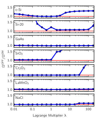
Figure 1: (Color online) Ratio of $\Omega^{\rm OPF}$ and $\Omega^{\rm GM}$ as a function of Lagrange multiplier $\lambda$ on a logarithmic scale.

IV.1 Insight gained from the matrix $W$

To demonstrate the kind of insight that can be gained from analyzing the $W$ matrix, we analyze here in more detail case of LaMnO₃ and Cr₂O₃. In both cases, $s$ and $p$ orbitals on the neighboring oxygen atoms outside the computational unit cell are included in $A^{(\mathbf{k})}$ in order to complete the octahedral coordination of the Cr and Mn atoms.

We studied LaMnO₃ in its low temperature $(\lesssim 135\textrm{K})$ A-AFM phase characterized by ferromagnetic ordering of the Mn spins in-plane and antiferromagnetic order between planes.Elemans et al. (1971) In addition to the magnetic order, Mn $d$ states are orbitally ordered, oxygen octahedra are tilted and Jahn-Teller distorted. In the following, we focus only on the two topmost spin-polarized bands below the Fermi level. Analyzing the $W$ matrix we see that the Wannier functions for the two topmost bands in LaMnO₃ are dominantly composed of rotated $d_{z^{2}}$ components on Mn that are oriented perpendicular to each other. This can be seen also by analyzing the $W$ matrix for these two WFs,

$$\ket{1} \approx 0.5\ket{\mathrm{Mn1};d_{z^{2}}}+0.6\ket{\mathrm{Mn1};d_{xy}}$$

$$\ket{2} \approx 0.6\ket{\mathrm{Mn2};d_{z^{2}}}-0.5\ket{\mathrm{Mn2};d_{xy}}.$$

Figure 2 shows a plot of these WFs for the top bands with isosurfaces in the left panels and contour plots in the right panels. The contours are plotted in the plane perpendicular to the $c$ axis, cutting through the Mn atom.

Furthermore, The $W$ matrix shows hybridization of the Mn $d$ states with the oxygen $p$ states, with the corresponding elements of $W$ having a magnitude of approximately 0.2 (three times smaller than for Mn $d$ states). The contribution of the $p$-like lobes (colored red) can be seen in the right panels of Fig. 2 as the large lobes near the center.

Now we analyze the case of Cr₂O₃ in more detail. Cr₂O₃ is an antiferromagnetic insulator with four Cr atoms in the primitive unit cell. Therefore, we expect each Cr³⁺ ion to nominally have three occupied $d$ orbitals of same spin. These three occupied $d$ orbitals on four Cr ions form a complex of $3\times 4=12$ isolated bands that make up the topmost valence bands. Again, analyzing the $W$ matrix we obtained within our approach we find that each of the twelve WFs is a particular linear combination of all five $d$ orbitals, all having the same spin component along the $z$ axis. In fact, there is a large degeneracy regarding the particular combination of $d$ orbitals that make up the WFs. For example, even slight change in $\lambda$ from 1 to 2 gives different linear combinations of $d$ orbitals, while the spread remains nearly the same (see Fig. 1). This observation is consistent with the fact that the choice of MLWFs is not always unique. This was first suggested in Ref. Marzari and Vanderbilt, 1997 for the case of LiCl. There it was found that an arbitrary rotation of the $sp^{3}$ orbitals on chlorine atoms has no effect on the total spread $\Omega$.

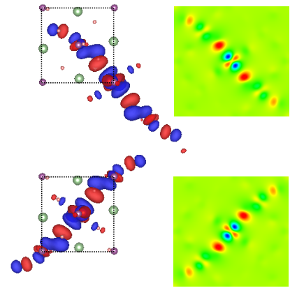
Figure 2: (Color online) Maximally localized Wannier functions of the two topmost valence bands in LaMnO₃. Isosurfaces of the WFs are shown on the left, looking down along the $c$ axis. The large green dots are La, medium purple dots are Mn, and small red dots are O. On the right, we show contour plots of the Wannier functions in the plane perpendicular to the $c$ axis, cutting through the Mn atom.

V Summary

We present an automated procedure for constructing maximally localized Wannier functions for an isolated group of bands. The extension of our method to the case of entangled bands will be the subject of future work.

Instead of having to guess functions (initial projections) that approximate the MLWFs as in Ref. Marzari and Vanderbilt, 1997, our approach only requires as input a set of functions that overspan the space of MLWFs. In practice, this can rather easily be achieved by selecting an appropriate set of valence atomiclike functions.

Appendix A Spread functional

Here we express components of the spread $\Omega$, corresponding to $N$ composite bands, as a function of the overlap matrices $m^{(\mathbf{k},\mathbf{b})}$ following Ref. Marzari and Vanderbilt, 1997,

$$\begin{split}\Omega_{\text{I}}&=\frac{1}{N_{\mathbf{k}}}\sum_{\mathbf{k},\mathbf{b}}w_{\mathbf{b}}\quantity(N-\sum_{ij}\absolutevalue{m^{(\mathbf{k},\mathbf{b})}_{ij}}^{2}),\\ \Omega_{\text{D}}&=\frac{1}{N_{\mathbf{k}}}\sum_{\mathbf{k},\mathbf{b}}w_{\mathbf{b}}\sum_{i}\quantity(-\textrm{Im}\,\ln m^{(\mathbf{k},\mathbf{b})}_{ii}-\mathbf{b}\cdot\overline{\mathbf{r}}_{i})^{2},\\ \Omega_{\text{OD}}&=\frac{1}{N_{\mathbf{k}}}\sum_{\mathbf{k},\mathbf{b}}w_{\mathbf{b}}\sum_{i\neq j}\absolutevalue{m^{(\mathbf{k},\mathbf{b})}_{ij}}^{2}.\end{split}$$ (41)

The $w_{\mathbf{b}}$ are the weights of the $\mathbf{b}$ vectors connecting neighboring $\mathbf{k}$ points (see Sec. 2.1 of Ref. 9), while

$$\overline{\mathbf{r}}_{i}=\frac{1}{N_{\mathbf{k}}}\sum_{\mathbf{k},\mathbf{b}}w_{\mathbf{b}}\mathbf{b}\imaginary\,\ln m^{(\mathbf{k},\mathbf{b})}_{ii}.$$ (42)

We note that the diagonal and off-diagonal parts of the spread depend only on the diagonal and off-diagonal components of the overlap matrices, respectively. Combining the invariant and off-diagonal parts of the spread gives an expression that depends only on the diagonal components of the overlap matrices,

$$\begin{split}\Omega_{\text{I},\text{OD}}&=\Omega_{\text{I}}+\Omega_{\text{OD}}\\ &=\frac{1}{N_{\mathbf{k}}}\sum_{\mathbf{k},\mathbf{b}}w_{\mathbf{b}}\sum_{i=1}^{N}\quantity[1-\absolutevalue{m^{(\mathbf{k},\mathbf{b})}_{ii}}^{2}].\end{split}$$ (43)

Appendix B Codiagonalization algorithm

In the main text, the construction of localized Wannier functions is recast into the following mathematical problem. Given a set of large $M\!\times\!M$ matrices $X^{(\alpha)}$, we wish to find a single rectangular semiunitary $M\!\times\!N$ matrix $W$ such that the set of small $N\!\times\!N$ matrices $W^{\dagger}X^{(\alpha)}W$ minimize the Lagrangian $\mathcal{L}$, defined in Eq. (40),

$$\sum_{\alpha}t^{(\alpha)}\sum_{i=1}^{N}\absolutevalue{\quantity[W^{\dagger}X^{(\alpha)}W]_{ii}}^{2}.$$ (44)

We parametrize the semiunitary matrix $W$ as follows. First, we define $W$ to be first $N$ columns of an $M\!\times\!M$ unitary matrix $\widetilde{W}$. Second, we iteratively parametrize the enlarged matrix $\widetilde{W}$ as a product (post-multiplication) of Givens rotations,Golub and Van Loan (1996)

$$\widetilde{W}=\prod_{l=1}^{L}\prod_{i=1}^{N}\prod_{j=i+1}^{M}R_{l}[i,j,\theta,\phi].$$ (45)

Here integer $l$ denotes a particular iteration in the expansion.

A Givens rotation $R[i,j,\theta,\phi]$ is the most general unitary matrix that acts only on $i$-th and $j$-th rows and columns. Therefore, we parametrize $R[i,j,\theta,\phi]$ with two angles $\theta$ and $\phi$ as a matrix equal to the identity matrix for all elements except for the $ii$, $ij$, $ji$, and $jj$ elements,

$$\begin{pmatrix}R_{ii}&R_{ij}\\ R_{ji}&R_{jj}\end{pmatrix}=\begin{pmatrix}\cos\theta&e^{i\phi}\sin\theta\\ -e^{-i\phi}\sin\theta&\cos\theta\end{pmatrix}.$$ (46)

The only diagonal elements of $X^{(\alpha)}$ affected by $R[i,j,\theta,\phi]$ are $X^{(\alpha)}_{ii}$ and $X^{(\alpha)}_{jj}$. Therefore there is no need to include in Eq. (45) cases when both $i$ and $j$ are larger than $N$, since that operation will have no effect on the Lagrangian. In addition, we don’t consider cases when $j<i$ since that transformation is captured by $j>i$. With this parametrization an arbitrary unitary matrix $\widetilde{W}$ can be approximated to an arbitrary precision with large enough number of iterations, $L$.

Let us now see how does a single Givens rotation affect the Lagrangian. For a Givens rotation $R[i,j,\theta,\phi]$, the sum of the weighted square moduli of the diagonal elements ($ii$ and $jj$) of a set of rotated matrices $R^{\dagger}X^{(\alpha)}R$ areSørensen et al. (2012)

$$\sum_{\alpha}t^{(\alpha)}\quantity|\quantity[R^{\dagger}X^{(\alpha)}R]_{ii}|^{2} =\mathbf{x}^{\intercal}Q\mathbf{x}+\mathbf{p}^{\intercal}\mathbf{x}+c$$ (47)

$$\sum_{\alpha}t^{(\alpha)}\quantity|\quantity[R^{\dagger}X^{(\alpha)}R]_{jj}|^{2} =\mathbf{x}^{\intercal}Q\mathbf{x}-\mathbf{p}^{\intercal}\mathbf{x}+c$$ (48)

where

$$\mathbf{x}^{\intercal}=\quantity(\cos 2\theta,\sin 2\theta\cos\phi,\sin 2\theta\sin\phi)$$ (49)

is a vector with unit norm by construction. The coefficients of the quadratic forms above [Eqs. (47) and (48)] depend only on the $ii$, $ij$, $ji$, and $jj$ components of the $X^{(\alpha)}$ matrices

$$\begin{split}Q&=\sum_{\alpha}t^{(\alpha)}\real\quantity[\mathbf{z}^{(\alpha)}\mathbf{z}^{(\alpha)\dagger}]\\ \mathbf{p}&=\sum_{\alpha}t^{(\alpha)}\real\quantity[\quantity(X^{(\alpha)}_{ii}+X^{(\alpha)}_{jj})^{*}\mathbf{z}^{(\alpha)}]\\ c&=\sum_{\alpha}\frac{1}{4}t^{(\alpha)}\quantity|X^{(\alpha)}_{ii}+X^{(\alpha)}_{jj}|^{2}\end{split}$$ (50)

where

$$\mathbf{z}^{(\alpha)}=\frac{1}{2}\begin{bmatrix}X^{(\alpha)}_{ii}-X^{(\alpha)}_{jj}\\ -\quantity(X^{(\alpha)}_{ij}+X^{(\alpha)}_{ji})\\ i\quantity(X^{(\alpha)}_{ij}-X^{(\alpha)}_{ji})\\ \end{bmatrix}.$$ (51)

We now consider two cases. First, if $j\leq N$ both the $ii$ and $jj$ diagonal elements enter the Lagrangian $\mathcal{L}$ so we need to find $\mathbf{x}$ that minimizes the sum of Eqs. (47) and (48),

$$\begin{split}\sum_{\alpha}&\,t^{(\alpha)}\quantity|\quantity[R^{\dagger}X^{(\alpha)}R]_{ii}|^{2}+t^{(\alpha)}\quantity|\quantity[R^{\dagger}X^{(\alpha)}R]_{jj}|^{2}\\ &=2\mathbf{x}^{\intercal}Q\mathbf{x}+2c.\end{split}$$ (52)

This is a quadratic programming problem with the constraint that $\absolutevalue{\mathbf{x}}=1$. Here, the Lagrangian is simply minimized for $\mathbf{x}$ that is the normalized eigenvector corresponding to the minimal eigenvalue of $Q$. For numerical stability, if the first component of $\mathbf{x}$ (i.e., $\cos 2\theta$) happens to be negative we choose $-\mathbf{x}$ instead of $\mathbf{x}$.

In the second case $(j\!>\!N)$, only the $ii$ diagonal components enters the Lagrangian $\mathcal{L}$ so we need to find $\mathbf{x}$ that minimizes Eq. (47),

$$\mathbf{x}^{\intercal}Q\mathbf{x}+\mathbf{p}^{\intercal}\mathbf{x}+c.\\$$ (53)

The solution of this problem is discussed in Ref. 16 within the context of matrix codiagonalization. However we find the general quadratic programming solution from Ref. 23 more numerically stable. Following Ref. 23, we first find the minimal eigenvalue $\chi_{\mathrm{min}}$ of the quadratic eigenvalue problem (QEP)

$$\quantity(\chi^{2}A_{2}+\chi A_{1}+A_{0})\mathbf{x}=0,$$ (54)

with

$$\begin{split}&A_{2}=I_{3}\\ &A_{1}=-2Q\\ &A_{0}=Q^{2}-\frac{1}{4}\mathbf{p}\mathbf{p}^{\intercal}.\end{split}$$ (55)

The QEP is linearized by introducing

$$\widetilde{\mathbf{x}}=\begin{pmatrix}\chi\mathbf{x}\\ \mathbf{x}\end{pmatrix}$$ (56)

yielding a generalized eigenvalue problem

$$A\widetilde{\mathbf{x}}=\chi B\widetilde{\mathbf{x}},$$ (57)

with

$$\begin{split}&A=\matrixquantity*(A_{1}\hfil&&A_{0}\\ -I_{3}&&0)\\ &B=\matrixquantity*(A_{2}\hfil&&0\\ 0&&I_{3}).\end{split}$$ (58)

This generalized eigenvalue problem we solve using standard linear algebra techniques. The solution $\mathbf{x}$ that minimizes Eq. 53 depends on whether $\chi_{\mathrm{min}}$ is in the spectrum of $Q$ or not.

If $\chi_{\mathrm{min}}$ is not in the spectrum (i.e. not an eigenvalue) of $Q$ then the solution is $\mathbf{x}=\quantity(Q-\chi_{\mathrm{min}}I)^{-1}(-\mathbf{p}/2)$. If $\chi_{\mathrm{min}}$ is an eigenvalue of $Q$ we first define

$$\mathbf{u}:=\quantity(Q-\chi_{\mathrm{min}}I)^{+}\quantity(-\mathbf{p}/2).$$ (59)

Here symbol ⁺ denotes a matrix pseudoinverse. A nontrivial solution to Eq. 53 exists only when the following conditions are satisfied:

$$(Q-\chi_{\mathrm{min}}I)\mathbf{u}=-\mathbf{p}/2\quad\mathrm{and}\quad\absolutevalue{\mathbf{u}}\leq 1.$$ (60)

Finally, if $\absolutevalue{\mathbf{u}}=1$, then the solution is $\mathbf{x}=\mathbf{u}$. Otherwise ($\absolutevalue{\mathbf{u}}<1$) the solution is $\mathbf{x}=\mathbf{u}+\bm{\xi}$. Here $\bm{\xi}$ is an eigenvector of $Q$ corresponding to $\chi_{\mathrm{min}}$ chosen so that $\absolutevalue{\bm{\xi}}^{2}=1-\absolutevalue{\mathbf{u}}^{2}$.

Once the $\mathbf{x}$ is found for a given $(i,j)$ in either of the two approaches we determine the corresponding angles $(\theta,\phi)$ from Eq. (49) and construct the Givens rotation $R[i,j,\theta,\phi]$. Next we update at each iteration the matrix $\widetilde{W}$ according to the postmultiplication parametrization from Eq. (45),

$$\begin{split}\widetilde{W}&\rightarrow\widetilde{W}R.\end{split}$$ (61)

This iterative procedure over $i$, $j$, and $l$ continues until the Lagrangian converges.

References

- Marzari et al. (2012) N. Marzari, A. A. Mostofi, J. R. Yates, I. Souza, and D. Vanderbilt, Rev. Mod. Phys. 84, 1419 (2012).
- Wu et al. (2006) X. Wu, O. Diéguez, K. M. Rabe, and D. Vanderbilt, Phys. Rev. Lett. 97, 107602 (2006).
- Yates et al. (2007) J. R. Yates, X. Wang, D. Vanderbilt, and I. Souza, Phys. Rev. B 75, 195121 (2007).
- Giustino et al. (2007) F. Giustino, M. L. Cohen, and S. G. Louie, Phys. Rev. B 76, 165108 (2007).
- Noffsinger et al. (2010) J. Noffsinger, F. Giustino, B. D. Malone, C.-H. Park, S. G. Louie, and M. L. Cohen, Comput. Phys. Commun. 181, 2140 (2010).
- Pizzi et al. (2014) G. Pizzi, D. Volja, B. Kozinsky, M. Fornari, and N. Marzari, Comput. Phys. Commun. 185, 422 (2014).
- Marzari and Vanderbilt (1997) N. Marzari and D. Vanderbilt, Phys. Rev. B 56, 12847 (1997).
- Souza et al. (2001) I. Souza, N. Marzari, and D. Vanderbilt, Phys. Rev. B 65, 035109 (2001).
- Mostofi et al. (2008) A. A. Mostofi, J. R. Yates, Y.-S. Lee, I. Souza, D. Vanderbilt, and N. Marzari, Comput. Phys. Commun. 178, 685 (2008).
- Jain et al. (2013) A. Jain, S. P. Ong, G. Hautier, W. Chen, W. D. Richards, S. Dacek, S. Cholia, D. Gunter, D. Skinner, G. Ceder, and K. A. Persson, APL Mater. 1, 011002 (2013).
- Thygesen et al. (2005a) K. S. Thygesen, L. B. Hansen, and K. W. Jacobsen, Phys. Rev. Lett. 94, 026405 (2005a).
- Thygesen et al. (2005b) K. S. Thygesen, L. B. Hansen, and K. W. Jacobsen, Phys. Rev. B 72, 125119 (2005b).
- Sakuma (2013) R. Sakuma, Phys. Rev. B 87, 235109 (2013).
- Gygi et al. (2003) F. Gygi, J.-L. Fattebert, and E. Schwegler, Comput. Phys. Commun. 155, 1 (2003).
- Cardoso and Souloumiac (1996) J.-F. Cardoso and A. Souloumiac, SIAM J. Matrix Anal. and Appl. 17, 161 (1996).
- Sørensen et al. (2012) M. Sørensen, L. D. Lathauwer, S. Icart, and L. Deneire, Signal Process. 92, 617 (2012).
- Xiang et al. (2013) H. J. Xiang, B. Huang, E. Kan, S.-H. Wei, and X. G. Gong, Phys. Rev. Lett. 110, 118702 (2013).
- Giannozzi et al. (2009) P. Giannozzi, S. Baroni, N. Bonini, M. Calandra, R. Car, C. Cavazzoni, D. Ceresoli, G. L. Chiarotti, M. Cococcioni, I. Dabo, A. Dal Corso, S. de Gironcoli, S. Fabris, G. Fratesi, R. Gebauer, U. Gerstmann, C. Gougoussis, A. Kokalj, M. Lazzeri, L. Martin-Samos, N. Marzari, F. Mauri, R. Mazzarello, S. Paolini, A. Pasquarello, L. Paulatto, C. Sbraccia, S. Scandolo, G. Sclauzero, A. P. Seitsonen, A. Smogunov, P. Umari, and R. M. Wentzcovitch, J. Phys.: Condens. Matter 21, 395502 (2009).
- Vanderbilt (1990) D. Vanderbilt, Phys. Rev. B 41, 7892 (1990).
- Garrity et al. (2014) K. F. Garrity, J. W. Bennett, K. M. Rabe, and D. Vanderbilt, Comput. Mater. Sci. 81, 446 (2014).
- Elemans et al. (1971) J. B. Elemans, B. V. Laar, K. V. D. Veen, and B. Loopstra, J. Solid State Chem. 3, 238 (1971).
- Golub and Van Loan (1996) G. H. Golub and C. F. Van Loan, Matrix Computations, 3rd ed. (Johns Hopkins University Press, Baltimore, MD, 1996).
- Gander et al. (1989) W. Gander, G. H. Golub, and U. von Matt, Linear Alg. Appl. 114-115, 815 (1989).