Mechanical balance laws for fully nonlinear and weakly dispersive water waves

Abstract.

The Serre-Green-Naghdi system is a coupled, fully nonlinear system of dispersive evolution equations which approximates the full water wave problem. The system is known to describe accurately the wave motion at the surface of an incompressible inviscid fluid in the case when the fluid flow is irrotational and two-dimensional. The system is an extension of the well known shallow-water system to the situation where the waves are long, but not so long that dispersive effects can be neglected.

In the current work, the focus is on deriving mass, momentum and energy densities and fluxes associated with the Serre-Green-Naghdi system. These quantities arise from imposing balance equations of the same asymptotic order as the evolution equations. In the case of an even bed, the conservation equations are satisfied exactly by the solutions of the Serre-Green-Naghdi system. The case of variable bathymetry is more complicated, with mass and momentum conservation satisfied exactly, and energy conservation satisfied only in a global sense. In all cases, the quantities found here reduce correctly to the corresponding counterparts in both the Boussinesq and the shallow-water scaling.

One consequence of the present analysis is that the energy loss appearing in the shallow-water theory of undular bores is fully compensated by the emergence of oscillations behind the bore front. The situation is analyzed numerically by approximating solutions of the Serre-Green-Naghdi equations using a finite-element discretization coupled with an adaptive Runge-Kutta time integration scheme, and it is found that the energy is indeed conserved nearly to machine precision. As a second application, the shoaling of solitary waves on a plane beach is analyzed. It appears that the Serre-Green-Naghdi equations are capable of predicting both the shape of the free surface and the evolution of kinetic and potential energy with good accuracy in the early stages of shoaling.

1. Introduction

In this paper we study mechanical balance laws for fully nonlinear and dispersive shallow-water waves. In particular, the Serre-Green-Naghdi (SGN) system of equations with variable bathymetry is considered. This system was originally derived for one-dimensional waves over a horizontal bottom in 1953 by F. Serre [1, 2]. Several years later, the same system was rederived by Su and Gardner [3]. In 1976, Green and Naghdi [4] derived a two-dimensional fully nonlinear and weakly dispersive system for an uneven bottom while in one spatial dimension Seabra-Santos et al. [5] derived the generalization of the Serre system with variable bathymetry. Lannes and Bonneton derived several other systems including the SGN equations using a new formulation of the water wave problem, [6]. For more information and generalizations of the SGN equations we refer to [7] and the references therein, while we refer to the paper by Barthélemy [8] for an extensive review.

The Serre-Green-Naghdi (SGN) system and several variants of it are extensively used in coastal modeling [9, 10, 11, 7]. In the present contribution, the focus is on one aspect of the equations which has not received much attention so far, namely the derivation and use of associated mechanical balance equations, and in particular a differential energy balance equation. While it is known that the equations admit four local conservation equations if the bed is even [12], it appears that the connection to mechanical balance laws of the original Euler equations has not been firmly established so far. Here we show that the first three conservation laws of the Serre-Green-Naghdi (SGN) equations arise as approximations of mechanical balance laws in the context of the Euler equations, both in the case of even beds, and in the case of nontrivial bathymetry. The fourth conservation law has been shown to arise from a kinematic identity similar to Kelvin’s circulation theorem [13].

Let us first review some modeling issues regarding the Serre-Green-Naghdi (SGN) system. Suppose $a$ denotes a typical amplitude, and $l$ a typical wavelength of a wavefield under study. Suppose also that $b_{0}$ represents the average water depth. In order to be a valid description of such a situation, the SGN equations require the shallow water condition, $\beta\doteq b_{0}^{2}/l^{2}\ll 1$. In contrast, the range of validity of the weakly nonlinear and weakly dispersive Boussinesq equations is limited to waves with small amplitude and large wavelength, i.e. $\alpha\doteq a/b_{0}\ll 1$ and $\beta\ll 1$. In this scaling regime, one also finds the weakly nonlinear, fully dispersive Whitham equation [7, 14, 15].

The SGN equations can be derived by depth-averaging the Euler equations and truncating the resulting set of equations at $\mathcal{O}(\beta^{2})$ without making any assumptions on the order of $\alpha$, other than $\alpha\leq\mathcal{O}(1)$.

In their dimensionless and scaled form the SGN equations can be written as

$$\eta_{t}+[h\bar{u}]_{x}=0\ ,$$ (1a)

$$\bar{u}_{t}+\bar{u}\bar{u}_{x}+g\eta_{x}+\frac{1}{h}\left[h^{2}\big{(}{\textstyle\frac{1}{3}}\mathcal{P}+{\textstyle\frac{1}{2}}\mathcal{Q}\big{)}\right]_{x}+b_{x}\big{(}{\textstyle\frac{1}{2}}\mathcal{P}+\mathcal{Q}\big{)}=0\ ,$$ (1b)

with $\mathcal{P}=h\left[\bar{u}_{x}^{2}-\bar{u}_{xt}-\bar{u}\bar{u}_{xx}\right]$ and $\mathcal{Q}=b_{x}(\bar{u}_{t}+\bar{u}\bar{u}_{x})+b_{xx}\bar{u}^{2}$, $x\in\mathbb{R}$, $t>0$, along with the initial conditions $h(x,0)=h_{0}(x)$, $\bar{u}(x,0)=\bar{u}_{0}(x)$. Here, $\eta=\eta(x,t)$ is the free surface displacement, while

$$h\doteq\eta-b\ ,$$ (2)

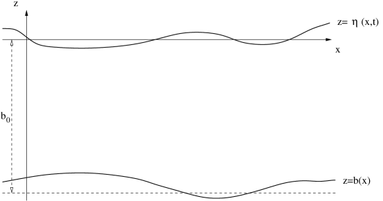
Figure 1. The geometry of the problem

denotes the total fluid depth. The unknown $\bar{u}=\bar{u}(x,t)$ is the depth-averaged horizontal velocity, and $\eta_{0}$, $\bar{u}_{0}$ are given real functions, such that $\eta_{0}-b>0$ for all $x\in\mathbb{R}$. In these variables, the location of the horizontal bottom is given by $z=b$ (cf. Figure 1). For a review of the derivation and the basic properties of this system we also refer to [8, 16].

In the case of small-amplitude waves, i.e. if $\beta\sim\alpha$, the SGN equations reduce to Peregrine’s system [17]. On the other hand, in the case of very long waves, i.e. $\beta\to 0$, the dispersive terms disappear, and the system reduces to the nondispersive shallow water equations.

The SGN system for waves over a flat bottom possesses solitary and cnoidal wave solutions given in closed form. For example, the solitary wave with speed $c_{s}$ can be written as

$$h_{s}(\xi)\doteq h_{s}(x,t)=a_{0}+a_{1}{\mathrm{sech}}^{2}(K_{s}\,\xi),$$ (3a)

$$u_{s}(\xi)\doteq u_{s}(x,t)=c_{s}\left(1-\frac{a_{0}}{h_{s}(\xi)}\right),$$ (3b)

where $\xi=x-c_{s}t$, $K_{s}=\sqrt{3a_{1}/4a_{0}^{2}c_{s}^{2}}$, $c_{s}=\sqrt{a_{0}+a_{1}}$, and $a_{0}>0$ and $a_{1}>0$. For more information about the solitary and cnoidal waves and their dynamical properties we refer to [8, 12, 18, 19, 20, 21].

It is important to note that the SGN system has a Hamiltonian structure, even in the case of two-dimensional waves over an uneven bed cf. [19, 22, 23, 24]. Specifically, any solution $(h,\bar{u})$ of (1) conserves the Hamiltonian functional

$$\mathcal{H}(t)=\frac{1}{2}\int_{-\infty}^{\infty}g\eta^{2}+h\bar{u}^{2}+h\left[h_{x}b_{x}+{\textstyle{1\over 2}}hb_{xx}+b_{x}^{2}\right]\bar{u}^{2}-{\textstyle{1\over 3}}\left[h^{3}\bar{u}_{x}\right]_{x}\bar{u}~{}dx\ ,$$ (4)

in the sense that $d\mathcal{H}(t)/dt=0$. Note however that (1a), (1b) are recovered only if a non-canonical symplectic structure matrix is used. While in many simplified models equations, the Hamiltonian functions does not represent the mechanical energy of the wave problem [25], in the case of SGN, the Hamiltonian does represent the approximate total energy of the wave system. Thus the Hamiltonian can be written in the form

$$\mathcal{H}(t)=\int_{-\infty}^{\infty}E(x,t)\,dx\ ,$$

where the integrand

$$E=\frac{1}{2}\left(g\eta^{2}+h\bar{u}^{2}+h\left[h_{x}b_{x}+{\textstyle{1\over 2}}hb_{xx}+b_{x}^{2}\right]\bar{u}^{2}-{\textstyle{1\over 3}}\left[h^{3}\bar{u}_{x}\right]_{x}\bar{u}\right)$$

is the depth-integrated energy density. In the present paper, we also identify a local depth-integrated energy flux $q_{E}$, such that an equation of the form

$$\frac{\partial E}{\partial t}+\frac{\partial{q_{E}}}{\partial x}=0\ ,$$ (5)

is satisfied approximately. The procedure of finding the quantities $E$ and $q_{E}$ follows a similar outline as the derivations in [26] for a class of Boussinesq systems and [27] for the KdV equation. Expressions for energy functionals associated to Boussinesq systems have also been developed in [28].

The analytical results are put to use in the study of undular bores. It is well known that the shallow-water theory for bores predicts an energy loss [29]. In an undular bore, the energy is thought to be disseminated through an increasing number of oscillations behind the bore, and the traditional point of view is that dissipation must also have an effect here [30, 31]. However, recent studies [32] have shown that if dispersion is included into the model equations, then the energy loss experienced by an undular bore can be accounted for without making appeal to dissipative mechanisms.

Indeed, it was argued in [32, 33] that the energy loss in an undular bore could be explained wholly within the realm of conservative dynamics by investigating a higher-order dispersive system, and monitoring the associated energy functional. However, there was a technical problem in the analysis in these works, as the energy functional was not the same as the one required by the more in-depth analysis in [26]. On the other hand, the energy functional found in [26] did not reduce to the shallow-water theory in the correct way. In the current contribution, it is our purpose to remedy this situation by using the SGN system which reduces in the correct way to the shallow-water equations, and also features exact energy conservation in the case of a flat bed.

The numerical method to be used is a standard Galerkin / Finite Element Method (FEM) for the SGN equations with reflective boundary conditions extending the numerical method presented in [34]. For the sake of completeness we mention that there are several numerical methods applied to boundary value problems of the SGN equations. For example finite volume [35, 36, 37], finite differences [16, 38, 39], spectral [36] and Galerkin methods [34, 40].

The paper is organized as follows: A review of the derivation of the SGN equations based on [8, 16] is presented in Section 2. The derivation of the mass, momentum and energy balance laws in the asymptotic order of the SGN equations is presented in Section 3. Applications to undular bores and solitary waves are discussed in Section 4. The numerical method to be used used in this paper is presented briefly in A.

2. The SGN equations over a variable bed

Before introducing the balance laws for the SGN equations, we briefly review the derivation of the SGN equations from the Euler equations following the work [8], but in the case of a general bathymetry. This well known derivation is included here to set the stage for the development of the approximate mechanical balance laws in the next section. We consider an inviscid and incompressible fluid, and assume that the fluid flow is irrotational and two-dimensional. Let $a_{0}$ be a typical amplitude, $l$ a typical wavelength and $b_{0}$ a typical water depth. We perform the change of variables $\tilde{x}=x/l$, $\tilde{z}=z/b_{0}$, $\tilde{t}=c_{0}t/l$, which yields non-dimensional independent variables identified by tildes, where $x$ represents the horizontal and $z$ the vertical coordinate. The limiting long-wave speed is defined by $c_{0}=\sqrt{gb_{0}}$, and $g$ denotes the acceleration due to gravity. The non-dimensional velocity components are defined by $\tilde{u}=u/\alpha c_{0}$, $\tilde{v}=v/\sqrt{\beta}\alpha c_{0}$, where $\alpha=a_{0}/b_{0}$ and $\beta=b_{0}^{2}/l^{2}$. Finally, the free surface deflection, bottom topography and pressure are non-dimensionalized by taking $\tilde{\eta}=\eta/a_{0}$, $\tilde{b}=b/b_{0}$, and $\tilde{p}=p/\rho gb_{0}$.

In non-dimensional variables, the free-surface problem is written as follows [41]: The momentum equations are

$$\alpha\tilde{u}_{\tilde{t}}+\alpha^{2}(\tilde{u}^{2})_{\tilde{x}}+\alpha^{2}(\tilde{u}\tilde{v})_{\tilde{z}}=-\tilde{p}_{\tilde{x}}\ ,$$ (6a)

$$\alpha\beta\tilde{v}_{\tilde{t}}+\alpha^{2}\beta\tilde{u}\tilde{v}_{\tilde{x}}+\alpha^{2}\beta\tilde{v}\tilde{v}_{\tilde{z}}=-\tilde{p}_{\tilde{z}}-1\ .$$ (6b)

The equation of continuity and the irrotationality are expressed by

$$\tilde{u}_{\tilde{x}}+\tilde{v}_{\tilde{z}}=0\ ,$$ (7a)

$$\tilde{u}_{\tilde{z}}-\beta\tilde{v}_{\tilde{x}}=0\ .$$ (7b)

The boundary conditions at the free surface and at the bottom are given by

$$\tilde{v} =\tilde{\eta}_{\tilde{t}}+\alpha\tilde{u}\tilde{\eta}_{\tilde{x}}, \tilde{z}=\alpha\tilde{\eta}(\tilde{x})\ ,\qquad\qquad\qquad\qquad\qquad$$ at (8a)

$$\tilde{p} =0, \tilde{z}=\alpha\tilde{\eta}(\tilde{x})\ ,$$ at (8b)

$$\tilde{v} =\tilde{b}_{\tilde{x}}\tilde{u}, \tilde{z}=\tilde{b}(\tilde{x})\ .$$ at (8c)

The first equation in the system (1) is obtained by integrating the equation of continuity over the total depth. The result is written in terms of the depth-averaged horizontal velocity

$$\bar{\tilde{u}}=\frac{1}{\tilde{h}}\int_{\tilde{b}}^{\alpha\tilde{\eta}}\tilde{u}~{}dz\ ,$$ (9)

in the form

$$\tilde{\eta}_{\tilde{t}}+[\tilde{h}\bar{\tilde{u}}]_{\tilde{x}}=0\ .$$ (10)

Using the boundary conditions (8a)-(8c), the continuity equation (10) and the depth-averaged momentum equation (6a) yields

$$\alpha\tilde{h}\bar{\tilde{u}}_{\tilde{t}}+\alpha^{2}\tilde{h}\bar{\tilde{u}}\bar{\tilde{u}}_{\tilde{x}}+\alpha^{2}\frac{\partial}{\partial\tilde{x}}\int_{\tilde{b}}^{\alpha\tilde{\eta}}\left(\tilde{u}^{2}-(\bar{\tilde{u}})^{2}\right)\,d\tilde{z}=-\int_{\tilde{b}}^{\alpha\tilde{\eta}}\tilde{p}_{\tilde{x}}\,d\tilde{z}\ .$$ (11)

Applying the Leibniz rule to the right-hand side of equation (11) yields

$$\int_{\tilde{b}}^{\alpha\tilde{\eta}}\tilde{p}_{\tilde{x}}\,d\tilde{z} =\frac{\partial}{\partial\tilde{x}}\big{(}\tilde{h}\bar{\tilde{p}}\big{)}-\alpha\eta_{\tilde{x}}\tilde{p}|_{\tilde{z}=\alpha\tilde{\eta}}+\tilde{b}_{\tilde{x}}\tilde{p}|_{\tilde{z}=\tilde{b}}$$

$$=\frac{\partial}{\partial\tilde{x}}\big{(}\tilde{h}\bar{\tilde{p}}\big{)}+\tilde{b}_{\tilde{x}}\tilde{p}|_{\tilde{z}=\tilde{b}}\ .$$ (12)

The momentum equation (6b) is rewritten as

$$\alpha\beta\Gamma(\tilde{x},\tilde{z},\tilde{t})=-1-\tilde{p}_{\tilde{z}}\ ,$$ (13)

where

$$\Gamma(\tilde{x},\tilde{z},\tilde{t})=\tilde{v}_{\tilde{t}}+\alpha\tilde{u}\tilde{v}_{\tilde{x}}+\alpha\tilde{v}\tilde{v}_{\tilde{z}}\ .$$ (14)

Integrating equation (13) from $\tilde{z}$ to $\alpha\tilde{\eta}$ yields

$$\tilde{p}(\tilde{x},\tilde{z},\tilde{t})=(\alpha\tilde{\eta}-\tilde{z})+\alpha\beta\int^{\alpha\tilde{\eta}}_{\tilde{z}}\Gamma(\tilde{x},\zeta,\tilde{t})\,d\zeta\ ,$$ (15)

and taking the mean value gives

$$\tilde{h}\bar{\tilde{p}}=\frac{1}{2}\tilde{h}^{2}+\alpha\beta\int_{\tilde{b}}^{\alpha\tilde{\eta}}\int_{\tilde{z}}^{\alpha\tilde{\eta}}\Gamma(\tilde{x},\zeta,\tilde{t})\,d\zeta\ d\tilde{z}\ .$$ (16)

Therefore, equation (11) can be written as

$$\bar{\tilde{u}}_{\tilde{t}}+\alpha\bar{\tilde{u}}\bar{\tilde{u}}_{\tilde{x}}+\tilde{\eta}_{\tilde{x}}+\frac{\beta}{\tilde{h}}\frac{\partial}{\partial\tilde{x}}\int_{\tilde{b}}^{\alpha\tilde{\eta}}(\tilde{z}-\tilde{b})\Gamma(\tilde{x},\tilde{z},\tilde{t})\,d\tilde{z}\\ +\frac{\beta}{\tilde{h}}\tilde{b}_{\tilde{x}}\int_{\tilde{b}}^{\alpha\tilde{\eta}}\Gamma(\tilde{x},\tilde{z},\tilde{t})\,d\tilde{z}=\frac{-\alpha}{\tilde{h}}\frac{\partial}{\partial\tilde{x}}\int_{\tilde{b}}^{\alpha\tilde{\eta}}\left(\tilde{u}^{2}-(\bar{\tilde{u}})^{2}\right)\,d\tilde{z}\ .$$

The non-dimensional velocity componens are given (cf. [16]) to first order by

$$\tilde{u}(\tilde{x},\tilde{z},\tilde{t})=\bar{\tilde{u}}(\tilde{x},\tilde{t})+\mathcal{O}(\beta)\ ,$$ (17)

and

$$\tilde{v}(\tilde{x},\tilde{z},\tilde{t})=-\big{(}\tilde{z}-\tilde{b}(\tilde{x})\big{)}\frac{\partial\bar{\tilde{u}}}{\partial\tilde{x}}+\bar{\tilde{u}}\frac{\partial\tilde{b}}{\partial\tilde{x}}+\mathcal{O}(\beta)\ .$$ (18)

As it was shown in [16], we can expand the velocity components using Taylor series in the vertical coordinate around the bottom. Denoting by $\tilde{u}^{b}$ and $\tilde{v}^{b}$, respectively, the horizontal and vertical velocities at the bottom, the bottom kinematic condition (8c) imposes that $\tilde{v}^{b}=\tilde{b}_{\tilde{x}}\tilde{u}^{b}$. In order to determine which terms should be kept to obtain an approximation for the velocity field, the incompressibility condition (7a) must hold to the same order in $\beta$ as the evolution equations. If the non-dimensional velocity components are given by

$$\tilde{u}(\tilde{x},\tilde{z},\tilde{t})=\tilde{u}^{b}(\tilde{x},\tilde{t})+\beta(\tilde{z}-\tilde{b})\left(\tilde{b}_{\tilde{x}}\tilde{u}_{\tilde{x}}^{b}+(\tilde{b}_{\tilde{x}}\tilde{u}^{b})_{\tilde{x}}\right)\\ -\frac{\beta}{2}(\tilde{z}-\tilde{b})^{2}\tilde{u}_{\tilde{x}\tilde{x}}^{b}+\mathcal{O}(\beta^{2})\ ,$$ (19)

$$\tilde{v}(\tilde{x},\tilde{z},\tilde{t})=\tilde{b}_{\tilde{x}}\tilde{u}^{b}+(\tilde{z}-\tilde{b})\left(-\tilde{u}_{\tilde{x}}^{b}+\beta(\tilde{b}_{\tilde{x}}(\tilde{u}^{b}\tilde{b}_{\tilde{x}})_{\tilde{x}}+\tilde{u}_{\tilde{x}}^{b}\tilde{b}_{\tilde{x}}^{2})\right)\\ -\frac{\beta}{2}(\tilde{z}-\tilde{b})^{2}\left(\tilde{b}_{\tilde{x}}\tilde{u}_{\tilde{x}\tilde{x}}^{b}+(\tilde{b}_{\tilde{x}}\tilde{u}_{\tilde{x}}^{b}+(\tilde{b}_{\tilde{x}}\tilde{u}^{b})_{\tilde{x}})_{\tilde{x}}\right)+\frac{\beta}{3!}(\tilde{z}-\tilde{b})^{3}\tilde{u}_{\tilde{x}\tilde{x}\tilde{x}}^{b}+\mathcal{O}(\beta^{2})\ ,$$

then the incompressibility condition (7a) holds to $\mathcal{O}(\beta^{2})$. Depth averaging (19) gives

$$\tilde{u}^{b}=\bar{\tilde{u}}-\frac{\beta}{2}\tilde{h}\left(\tilde{b}_{\tilde{x}}\bar{\tilde{u}}_{\tilde{x}}+(\tilde{b}_{\tilde{x}}\bar{\tilde{u}})_{\tilde{x}}\right)+\frac{\beta}{6}\tilde{h}^{2}\bar{\tilde{u}}_{\tilde{x}\tilde{x}}+\mathcal{O}(\beta^{2},\alpha\beta^{2})\ .$$

Thus the horizontal velocity is

$$\tilde{u}(\tilde{x},\tilde{z},\tilde{t})=\bar{\tilde{u}}-\beta\left(\tilde{b}_{\tilde{x}}\bar{\tilde{u}}_{\tilde{x}}+(\tilde{b}_{\tilde{x}}\bar{\tilde{u}})_{\tilde{x}}\right)\left(\frac{\tilde{h}}{2}-(\tilde{z}-\tilde{b})\right)\\ +\beta\left(\frac{\tilde{h}^{2}}{6}-\frac{1}{2}(\tilde{z}-\tilde{b})^{2}\right)\bar{\tilde{u}}_{\tilde{x}\tilde{x}}+\mathcal{O}(\beta^{2},\alpha\beta^{2})\ .$$ (20)

Taking squares in equation ( 20)

$$\tilde{u}^{2}(\tilde{x},\tilde{z},\tilde{t})=\bar{\tilde{u}}^{2}-\beta\left(\tilde{b}_{\tilde{x}}\bar{\tilde{u}}_{\tilde{x}}\bar{\tilde{u}}+(\tilde{b}_{\tilde{x}}\bar{\tilde{u}})_{\tilde{x}}\bar{\tilde{u}}\right)\left(\tilde{h}-2(\tilde{z}-\tilde{b})\right)+\\ \beta\left(\frac{\tilde{h}^{2}}{2}-(\tilde{z}-\tilde{b})^{2}\right)\bar{\tilde{u}}\bar{\tilde{u}}_{\tilde{x}\tilde{x}}+\mathcal{O}(\beta^{2},\alpha\beta^{2})\ .$$ (21)

Integrating equation (21) from $\tilde{b}$ to $\alpha\tilde{\eta}$ and after some simplifications it follows that

$$\int_{\tilde{b}}^{\alpha\tilde{\eta}}\left(\tilde{u}^{2}-(\bar{\tilde{u}})^{2}\right)\,d\tilde{z}=\mathcal{O}(\beta^{2},\alpha\beta^{2})\ ,$$ (22)

and that

$$\Gamma(\tilde{x},\tilde{z},\tilde{t})=(\tilde{z}-\tilde{b})\left[\alpha\bar{\tilde{u}}_{\tilde{x}}^{2}-\bar{\tilde{u}}_{\tilde{x}\tilde{t}}-\alpha\bar{\tilde{u}}\bar{\tilde{u}}_{\tilde{x}\tilde{x}}\right]+\\ +\tilde{b}_{\tilde{x}}(\bar{\tilde{u}}_{\tilde{t}}+\alpha\bar{\tilde{u}}\bar{\tilde{u}}_{\tilde{x}})+\alpha\tilde{b}_{\tilde{x}\tilde{x}}\bar{\tilde{u}}^{2}+\mathcal{O}(\beta,\alpha\beta)\ .$$ (23)

Evaluating the integrals $\int_{\tilde{b}}^{\alpha\tilde{\eta}}\Gamma\,d\tilde{z}$ and $\int_{\tilde{b}}^{\alpha\tilde{\eta}}(\tilde{z}-\tilde{b})\Gamma\,d\tilde{z}$ yields

$$\int_{\tilde{b}}^{\alpha\tilde{\eta}}\Gamma\,d\tilde{z}=\frac{1}{2}\tilde{h}\tilde{\mathcal{P}}+\tilde{h}\tilde{\mathcal{Q}}\ ,$$ (24)

and

$$\int_{\tilde{b}}^{\alpha\tilde{\eta}}(\tilde{z}-\tilde{b})\Gamma\,d\tilde{z}=\frac{1}{3}\tilde{h}^{2}\tilde{\mathcal{P}}+\frac{1}{2}\tilde{h}^{2}\tilde{\mathcal{Q}}\ ,$$ (25)

where

$$\tilde{\mathcal{P}}=\tilde{h}\left[\alpha\bar{\tilde{u}}_{\tilde{x}}^{2}-\bar{\tilde{u}}_{\tilde{x}\tilde{t}}-\alpha\bar{\tilde{u}}\bar{\tilde{u}}_{\tilde{x}\tilde{x}}\right]\ ,$$ (26)

and

$$\tilde{\mathcal{Q}}=\tilde{b}_{\tilde{x}}\left(\bar{\tilde{u}}_{\tilde{t}}+\alpha\bar{\tilde{u}}\bar{\tilde{u}}_{\tilde{x}}\right)+\tilde{b}_{\tilde{x}\tilde{x}}\bar{\tilde{u}}^{2}\ .$$ (27)

Finally we find the second equation of the system as

$$\bar{\tilde{u}}_{\tilde{t}}+\alpha\bar{\tilde{u}}\bar{\tilde{u}}_{\tilde{x}}+\tilde{\eta}_{\tilde{x}}+\frac{\beta}{\tilde{h}}\frac{\partial}{\partial\tilde{x}}\left\{\Big{(}{\textstyle\frac{1}{3}}\tilde{\mathcal{P}}+{\textstyle\frac{1}{2}}\tilde{\mathcal{Q}}\Big{)}\tilde{h}^{2}\right\}+\beta\tilde{b}_{\tilde{x}}\Big{(}{\textstyle\frac{1}{2}}\tilde{\mathcal{P}}+\tilde{\mathcal{Q}}\Big{)}=\mathcal{O}(\alpha\beta^{2})\ .$$

By setting the right-hand side equal to zero, and writing the variables in dimensional form the system reads

$$\eta_{t}+[h\bar{u}]_{x}=0\ ,$$ (28a)

$$\bar{u}_{t}+\bar{u}\bar{u}_{x}+g\eta_{x}+\frac{1}{h}\left[h^{2}\big{(}{\textstyle\frac{1}{3}}\mathcal{P}+{\textstyle\frac{1}{2}}\mathcal{Q}\big{)}\right]_{x}+b_{x}\big{(}{\textstyle\frac{1}{2}}\mathcal{P}+\mathcal{Q}\big{)}=0\,,$$ (28b)

where $\mathcal{P}=h\left[\bar{u}_{x}^{2}-\bar{u}_{xt}-\bar{u}\bar{u}_{xx}\right]$ and $\mathcal{Q}=b_{x}(\bar{u}_{t}+\bar{u}\bar{u}_{x})+b_{xx}\bar{u}^{2}.$

In order to determine which terms should be kept for the velocity field at a certain order of approximation, the incompressibility condition (7a) can be used. Then, the dimensional form of the water particle velocities at any location $(x,z)$ in the vertical plane become

$$u=\bar{u}+\left(\frac{h^{2}}{6}-\frac{z^{2}}{2}\right)\bar{u}_{xx}\ ,$$ (29a)

$$v=-z\bar{u}_{x}\ .$$ (29b)

As it was mentioned before, system (1a) and (1b) reduces to the shallow water system when $\beta\rightarrow 0$ and to the classical Boussinesq system when $\beta\sim\alpha$.

An asymptotic expression for the pressure $\tilde{p}(\tilde{x},\tilde{z},\tilde{t})$ can be obtained by substituting formula (23) into (15). Such a formula was derived in [42] in the form

$$\tilde{p}(\tilde{x},\tilde{z},\tilde{t})=\alpha\tilde{\eta}-\tilde{z}++\frac{\alpha\beta}{2}\left[-\bar{\tilde{u}}_{\tilde{x}\tilde{t}}-\alpha\bar{\tilde{u}}\bar{\tilde{u}}_{\tilde{x}\tilde{x}}+\alpha\bar{\tilde{u}}_{\tilde{x}}^{2}\right]\left(\tilde{h}^{2}-(\tilde{z}-\tilde{b})^{2}\right)\\ +\alpha\beta\left(\alpha\tilde{b}_{\tilde{x}\tilde{x}}\bar{\tilde{u}}^{2}+\alpha\tilde{b}_{\tilde{x}}\bar{\tilde{u}}\bar{\tilde{u}}_{\tilde{x}}+\tilde{b}_{\tilde{x}}\bar{\tilde{u}}_{\tilde{t}}\right)(\alpha\tilde{\eta}-\tilde{z})+\mathcal{O}(\alpha\beta^{2})\ .$$ (30)

3. Mechanical balance laws for the SGN equations

In this section we derive the mechanical balance laws such as the mass, momentum and energy conservation for the SGN equations extending the results related to some Boussinesq systems found in [26]. The balance laws consist of terms of the same asymptotic order as in the SGN equations. We start with the conservation of mass.

3.1. Mass balance

We investigate the mass conservation properties of equations (28a) and (28b). Our starting point is the total mass of the fluid contained in a control volume of unit width, bounded by the lateral sides of the interval $[x_{1},x_{2}]$, and by the free surface and the bottom. This mass is given by

$$\mathcal{M}=\int_{x_{1}}^{x_{2}}\int_{b}^{\eta}\rho\,dz\,dx\,.$$ (31)

According to the principle of mass conservation and the fact that there is no mass flux through the bottom or the free surface, mass conservation can be considered in terms of the flow variables as follows:

$$\frac{d}{dt}\int_{x_{1}}^{x_{2}}\int_{b}^{\eta}\rho\,dz\,dx=\left[\int_{b}^{\eta}\rho u(x,z,t)\,dz\right]_{x_{2}}^{x_{1}}\,.$$ (32)

In non-dimensional form this equation becomes

$$\frac{d}{d\tilde{t}}\int_{\tilde{x}_{1}}^{\tilde{x}_{2}}\int_{\tilde{b}}^{\alpha\tilde{\eta}}\,d\tilde{z}\,d\tilde{x}=\alpha\left[\int_{\tilde{b}}^{\alpha\tilde{\eta}}\tilde{u}(\tilde{x},\tilde{z},\tilde{t})\,d\tilde{z}\right]_{\tilde{x}_{2}}^{\tilde{x}_{1}}\ .$$ (33)

Substituting the expression (20) for $\tilde{u}$ and integrating with respect to $\tilde{z}$ yields

$$\frac{d}{d\tilde{t}}\int_{\tilde{x}_{1}}^{\tilde{x}_{2}}\tilde{h}d\tilde{x}=\alpha\left[\bar{\tilde{u}}\tilde{h}\right]_{\tilde{x}_{2}}^{\tilde{x}_{1}}+\mathcal{O}(\alpha\beta^{2})\ ,$$ (34)

where $\tilde{h}=\alpha\tilde{\eta}-\tilde{b}$ denotes the nondimensional total depth. Dividing (34) by $\tilde{x}_{2}-\tilde{x}_{1}$ and taking $\tilde{x}_{2}-\tilde{x}_{1}\rightarrow 0$ then the mass balance equation is written as

$$\tilde{h}_{\tilde{t}}+(\alpha\bar{\tilde{u}}\tilde{h})_{\tilde{x}}=\mathcal{O}(\alpha\beta^{2})\ .$$ (35)

Denoting the non-dimensional mass density by $\tilde{M}=\tilde{h}$ and the non-dimensional mass flux by $\tilde{q}_{M}=\alpha\bar{\tilde{u}}\tilde{h}$, then the mass balance is

$$\frac{\partial\tilde{M}}{\partial{\tilde{t}}}+\frac{\partial{\tilde{q}_{M}}}{\partial{\tilde{x}}}=\mathcal{O}(\alpha\beta^{2})\,.$$ (36)

Using the scaling $M=\rho b_{0}\tilde{M}$ and $q_{M}=\rho b_{0}c_{0}\tilde{q}_{M}$ the dimensional forms of mass density and mass flux are $M=\rho h$ and $q_{M}=\rho\bar{u}h$ respectively. Then the dimensional form of the mass balance is obtained by discarding the right-hand side of the scaled mass balance equation and using the unscaled quantities:

$$\frac{\partial M}{\partial t}+\frac{\partial q_{M}}{\partial x}=0\ .$$ (37)

It is noted that the mass balance is satisfied exactly by the solutions of the SGN system.

The expressions for mass density and the mass flux do not depend on the shape of the bottom topography, and in particular, they have the same form for both even and uneven beds. The dimensional form of (35) coincides with analogous formulas of the shallow-water wave system and the classical Boussinesq system [26]. While this may be expected, it should be pointed out that in the case of other asymptotically equivalent systems, mass conservation may be satisfied only to the same order as the order of the equations, [26].

3.2. Momentum Balance

The total horizontal momentum of a fluid of constant density $\rho$ contained in a control volume of the same type as in the previous section is

$$\mathcal{I}=\int_{x_{1}}^{x_{2}}\int_{b}^{\eta}\rho u\,dz~{}dx\,.$$ (38)

Conservation of momentum implies that the rate of change of $\mathcal{I}$ is equal to the net influx of momentum through the boundaries plus the net force at the boundary of the control volume. Therefore, the conservation of momentum is written

$$\frac{d}{dt}\int_{x_{1}}^{x_{2}}\int_{b}^{\eta}\rho u\,dz\,dx=-\int_{x_{1}}^{x_{2}}pb_{x}~{}dx\\ +\left[\int_{b}^{\eta}\rho u^{2}(x,z)\,dz+\int_{b}^{\eta}pdz\right]_{x_{2}}^{x_{1}}\ .$$

Non-dimensionalization of this expression leads to

$$\alpha\frac{d}{d\tilde{t}}\int_{\tilde{x}_{1}}^{\tilde{x}_{2}}\int_{\tilde{b}}^{\alpha\tilde{\eta}}\tilde{u}\,d\tilde{z}\,d\tilde{x}=-\int_{\tilde{x}_{1}}^{\tilde{x}_{2}}\tilde{P}_{b}\tilde{b}_{\tilde{x}}~{}d\tilde{x}\\ +\left[\alpha^{2}\int_{\tilde{b}}^{\alpha\tilde{\eta}}\tilde{u}^{2}\,d\tilde{z}+\int_{\tilde{b}}^{\alpha\tilde{\eta}}\tilde{p}\,d\tilde{z}\right]_{\tilde{x}_{2}}^{\tilde{x}_{1}}\ ,$$

where $\tilde{P}_{b}$ denotes the pressure at the bottom $\tilde{P}_{b}=\tilde{h}+\frac{\alpha\beta}{2}[-\bar{\tilde{u}}_{\tilde{x}\tilde{t}}-\alpha\bar{\tilde{u}}\bar{\tilde{u}}_{\tilde{x}\tilde{x}}+\alpha\bar{\tilde{u}}_{\tilde{x}}^{2}]\tilde{h}^{2}+\alpha\beta(\alpha\tilde{b}_{\tilde{x}\tilde{x}}\bar{\tilde{u}}^{2}+\alpha\tilde{b}_{\tilde{x}}\bar{\tilde{u}}\bar{\tilde{u}}_{\tilde{x}}+\tilde{b}_{\tilde{x}}\bar{\tilde{u}}_{\tilde{t}})\tilde{h}$. Substituting the values of $\tilde{u}$ and $\tilde{p}$ from equations (20) and (15) and integrating with respect to $\tilde{z}$ yields

$$\alpha\frac{d}{d\tilde{t}}\int_{\tilde{x}_{1}}^{\tilde{x}_{2}}\bar{\tilde{u}}\tilde{h}d\tilde{x}=-\int_{\tilde{x}_{1}}^{\tilde{x}_{2}}\tilde{P}_{b}\tilde{b}_{\tilde{x}}\,d\tilde{x}\\ +\left[\alpha^{2}\bar{\tilde{u}}^{2}\tilde{h}+\frac{\tilde{h}^{2}}{2}-\frac{\alpha\beta}{3}\tilde{h}^{3}\Big{(}\bar{\tilde{u}}_{\tilde{x}\tilde{t}}+\alpha\bar{\tilde{u}}\bar{\tilde{u}}_{\tilde{x}\tilde{x}}-\alpha(\bar{\tilde{u}}_{\tilde{x}})^{2}\Big{)}\right]_{\tilde{x}_{2}}^{\tilde{x}_{1}}+\\ \left[\frac{\alpha\beta}{2}\tilde{h}^{2}\Big{(}\alpha\tilde{b}_{\tilde{x}\tilde{x}}\bar{\tilde{u}}^{2}+\tilde{b}_{\tilde{x}}(\alpha\bar{\tilde{u}}\bar{\tilde{u}}_{\tilde{x}}+\bar{\tilde{u}}_{\tilde{t}})\Big{)}\right]_{\tilde{x}_{2}}^{\tilde{x}_{1}}+\mathcal{O}(\alpha\beta^{2})\ .$$ (39)

Applying similar techniques used for the derivation of the mass balance equation we obtain the momentum balance equation in the form

$$\left(\alpha\bar{\tilde{u}}\tilde{h}\right)_{\tilde{t}}+\left(\alpha^{2}\bar{\tilde{u}}^{2}\tilde{h}+\frac{\tilde{h}^{2}}{2}-\frac{\alpha\beta}{3}\tilde{h}^{3}\Big{(}\bar{\tilde{u}}_{\tilde{x}\tilde{t}}+\alpha\bar{\tilde{u}}\bar{\tilde{u}}_{\tilde{x}\tilde{x}}-\alpha(\bar{\tilde{u}}_{\tilde{x}})^{2}\Big{)}\right)_{\tilde{x}}+\\ \left(\frac{\alpha\beta}{2}\tilde{h}^{2}\Big{(}\alpha\tilde{b}_{\tilde{x}\tilde{x}}\bar{\tilde{u}}^{2}+\tilde{b}_{\tilde{x}}(\alpha\bar{\tilde{u}}\bar{\tilde{u}}_{\tilde{x}}+\bar{\tilde{u}}_{\tilde{t}})\Big{)}\right)_{\tilde{x}}=-\tilde{P}_{b}\tilde{b}_{\tilde{x}}+\mathcal{O}(\alpha\beta^{2})\ .$$ (40)

If the non-dimensional momentum density is defined by

$$\tilde{I}=\alpha\bar{\tilde{u}}\tilde{h}\,$$ (41)

and the momentum flux plus pressure force is defined by

$$\tilde{q}_{I}=\alpha^{2}\bar{\tilde{u}}^{2}\tilde{h}+\frac{\tilde{h}^{2}}{2}-\frac{\alpha\beta}{3}\tilde{h}^{3}(\bar{\tilde{u}}_{\tilde{x}\tilde{t}}+\alpha\bar{\tilde{u}}\bar{\tilde{u}}_{\tilde{x}\tilde{x}}-\alpha(\bar{\tilde{u}}_{\tilde{x}})^{2})+\\ \frac{\alpha\beta}{2}\tilde{h}^{2}(\alpha\tilde{b}_{\tilde{x}\tilde{x}}\bar{\tilde{u}}^{2}+\tilde{b}_{\tilde{x}}(\alpha\bar{\tilde{u}}\bar{\tilde{u}}_{\tilde{x}}+\bar{\tilde{u}}_{\tilde{t}}))\,$$ (42)

then the momentum balance equation can be written as

$$\frac{\partial{\tilde{I}}}{\partial{\tilde{t}}}+\frac{\partial{\tilde{q}_{I}}}{\partial{\tilde{x}}}=-\tilde{P}_{b}\tilde{b}_{\tilde{x}}+\mathcal{O}(\alpha\beta^{2})\ .$$ (43)

Using the scaling $I=\rho c_{0}b_{0}\tilde{I}$ and $q_{I}=\rho c_{0}^{2}b_{0}\tilde{q_{I}}$, the dimensional forms of the momentum density and momentum flux per unit span are given by

$$I=\rho\bar{u}h\ ,$$ (44)

and

$$q_{I}=\rho\bar{u}^{2}h+\frac{\rho g}{2}h^{2}-\frac{\rho}{3}(\bar{u}_{xt}+\bar{u}\bar{u}_{xx}-\bar{u}_{x}^{2})h^{3}+\\ +\frac{\rho}{2}(b_{xx}\bar{u}^{2}+b_{x}(\bar{u}\bar{u}_{x}+\bar{u}_{t}))h^{2}\ ,$$ (45)

respectively. It turn out that the momentum conservation law is also satisfied exactly in the context of the SGN system. Indeed, if the momentum density is defined by (44), the momentum flux plus pressure force is defined by (45), and the pressure is defined by (30), then solutions of the SGN system also satisfy exactly the equation

$$\frac{\partial{I}}{\partial{t}}+\frac{\partial{q_{I}}}{\partial{x}}=-b_{x}p\ .$$ (46)

Note that if the bottom $b=-b_{0}$ is horizontal, then the last equation is homogeneous and does not depend on the pressure $p$.

Taking $\beta\rightarrow 0$ in the momentum balance equation (40), and using dimensional variables and horizontal bottom $b=-b_{0}$, the momentum density is unchanged, but the flux reduces to

$$q_{I}^{sw}=\rho\bar{u}^{2}h+\frac{\rho g}{2}h^{2}\ .$$ (47)

Thus it is plain that both the momentum density $I$ and flux $q_{I}$ reduce correctly to the nonlinear shallow water approximation. In the case $\beta\sim\alpha$ and a flat bottom, the quantities for the momentum balance law are $I=\rho\bar{u}(b_{0}+\eta)$ and $q_{I}=\rho b_{0}\bar{u}^{2}+\frac{\rho g}{2}h^{2}-\frac{\rho}{3}b_{0}^{3}\bar{u}_{xt}$, which agree with the corresponding quantities of the classical Boussinesq system.

3.3. Energy Balance

The total mechanical energy inside a control volume can be written as the sum of the kinetic and potential energy as

$$\mathcal{E}=\int_{x_{1}}^{x_{2}}\int_{b}^{\eta}\left\{{\textstyle\frac{\rho}{2}}(u^{2}+v^{2})+\rho gz\right\}\,dz\,dx\ .$$ (48)

The conservation energy can be expressed as

$$\frac{d}{dt}\int_{x_{1}}^{x_{2}}\int_{b}^{\eta}\left\{{\textstyle\frac{\rho}{2}}(u^{2}+v^{2})+\rho gz\right\}\,dz\,dx=\\ =\left[\int_{b}^{\eta}\left\{\left({\textstyle\frac{\rho}{2}}(u^{2}+v^{2})+\rho gz\right)u\,+uP\right\}\,dz\right]_{x_{2}}^{x_{1}}\ ,$$ (49)

and in non-dimensional variables as

$$\frac{d}{d\tilde{t}}\int_{\tilde{x}_{1}}^{\tilde{x}_{2}}\int_{\tilde{b}}^{\alpha\tilde{\eta}}\left\{{\textstyle\frac{\alpha^{2}}{2}}(\tilde{u}^{2}+\beta\tilde{v}^{2})\,+\tilde{z}\right\}\,d\tilde{z}\,d\tilde{x}=\\ \alpha\left[\int_{\tilde{b}}^{\alpha\tilde{\eta}}\left\{{\textstyle\frac{\alpha^{2}}{2}}(\tilde{u}^{3}+\beta\tilde{v}^{2}\tilde{u})+\tilde{z}\tilde{u}\,+\tilde{p}\tilde{u}\right\}\,d\tilde{z}\right]_{\tilde{x}_{2}}^{\tilde{x}_{1}}.$$ (50)

By substituting the expressions (17), (18) and (30) for $\tilde{u}$, $\tilde{v}$ and $\tilde{p}$ respectively, the energy balance equation takes the form

$$\frac{d}{d\tilde{t}}\int_{\tilde{x}_{1}}^{\tilde{x}_{2}}\left(\frac{\alpha^{2}}{2}\Big{(}\bar{\tilde{u}}^{2}+\beta{\tilde{b}_{\tilde{x}}}^{2}\bar{\tilde{u}}^{2}\Big{)}\tilde{h}-\frac{\alpha^{2}\beta}{2}\tilde{b}_{\tilde{x}}\tilde{h}^{2}\bar{\tilde{u}}\bar{\tilde{u}}_{\tilde{x}}+\right.\\ \left.\frac{\alpha^{2}\beta}{6}\tilde{h}^{3}\bar{\tilde{u}}_{\tilde{x}}^{2}+\frac{\tilde{h}^{2}}{2}+\tilde{b}\tilde{h}\right)d\tilde{x}=\left[\frac{\alpha^{3}}{2}\bar{\tilde{u}}^{3}\Big{(}1+\beta{\tilde{b}_{\tilde{x}}}^{2}\Big{)}\tilde{h}+\frac{\alpha}{2}\tilde{h}^{2}\bar{\tilde{u}}+\right.\\ \left.\alpha\tilde{b}\bar{\tilde{u}}\tilde{h}-\frac{\alpha^{3}\beta}{2}\tilde{b}_{\tilde{x}}\bar{\tilde{u}}_{\tilde{x}}\bar{\tilde{u}}^{2}\tilde{h}^{2}+\frac{\alpha^{3}\beta}{6}\bar{\tilde{u}}\bar{\tilde{u}}_{\tilde{x}}^{2}\tilde{h}^{3}\right]_{\tilde{x}_{2}}^{\tilde{x}_{1}}+\\ \left[\frac{\alpha}{2}\bar{\tilde{u}}\tilde{h}^{2}-\frac{\alpha^{2}\beta}{3}\tilde{h}^{3}\bar{\tilde{u}}\Big{(}\bar{\tilde{u}}_{\tilde{x}\tilde{t}}+\alpha\bar{\tilde{u}}\bar{\tilde{u}}_{\tilde{x}\tilde{x}}-\alpha\bar{\tilde{u}}_{\tilde{x}}^{2}\Big{)}\right.\\ \left.-\frac{\alpha^{2}\beta}{2}\Big{(}\alpha\tilde{b}_{\tilde{x}\tilde{x}}\bar{\tilde{u}}^{2}+\alpha\tilde{b}_{\tilde{x}}(\bar{\tilde{u}}\bar{\tilde{u}}_{\tilde{x}}+\bar{\tilde{u}}_{\tilde{t}})\Big{)}\tilde{h}^{2}\right]_{\tilde{x}_{2}}^{\tilde{x}_{1}}+\mathcal{O}(\alpha\beta^{2}).$$ (51)

The differential form of the energy balance equation is given by

$$\left(\frac{\alpha^{2}}{2}\Big{(}\bar{\tilde{u}}^{2}+\beta{\tilde{b}_{\tilde{x}}}^{2}\bar{\tilde{u}}^{2}\Big{)}\tilde{h}-\frac{\alpha^{2}\beta}{2}\tilde{b}_{\tilde{x}}\tilde{h}^{2}\bar{\tilde{u}}\bar{\tilde{u}}_{\tilde{x}}+\frac{\alpha^{2}\beta}{6}\tilde{h}^{3}\bar{\tilde{u}}_{\tilde{x}}^{2}+\frac{\tilde{h}^{2}}{2}+\tilde{b}\tilde{h}\right)_{\tilde{t}}\\ +\left(\frac{\alpha^{3}}{2}\bar{\tilde{u}}^{3}\tilde{h}+\frac{\alpha^{3}\beta}{3}\tilde{b}_{\tilde{x}}^{2}\bar{\tilde{u}}^{3}+\alpha\bar{\tilde{u}}\tilde{h}^{2}+\alpha\tilde{b}\bar{\tilde{u}}\tilde{h}-\frac{\alpha^{2}\beta}{3}\tilde{h}^{3}\bar{\tilde{u}}\Big{(}\bar{\tilde{u}}_{\tilde{x}\tilde{t}}+\alpha\bar{\tilde{u}}\bar{\tilde{u}}_{\tilde{x}\tilde{x}}\right.\\ \left.-\frac{3}{2}\alpha\bar{\tilde{u}}_{\tilde{x}}^{2}\Big{)}-\frac{\alpha^{3}\beta}{2}\tilde{b}_{\tilde{x}}\bar{\tilde{u}}_{\tilde{x}}\bar{\tilde{u}}^{2}\tilde{h}^{2}\right)_{\tilde{x}}\\ -\left(\frac{\alpha^{2}\beta}{2}\tilde{h}^{2}\Big{(}\alpha\tilde{b}_{\tilde{x}\tilde{x}}\bar{\tilde{u}}^{2}+\tilde{b}_{\tilde{x}}(\alpha\bar{\tilde{u}}\bar{\tilde{u}}_{\tilde{x}}+\bar{\tilde{u}}_{\tilde{t}})\Big{)}\right)_{\tilde{x}}=\mathcal{O}(\alpha\beta^{2})\ .$$ (52)

Considering the appropriate terms in the energy density and flux in (50) which are of order zero or one in the differential energy balance (51), we find that the non-dimensional energy density is

$$\tilde{E}=\frac{\alpha^{2}}{2}(\bar{\tilde{u}}^{2}+\beta{\tilde{b}_{\tilde{x}}}^{2}\bar{\tilde{u}}^{2})\tilde{h}-\frac{\alpha^{2}\beta}{2}\tilde{b}_{\tilde{x}}\tilde{h}^{2}\bar{\tilde{u}}\bar{\tilde{u}}_{\tilde{x}}+\frac{\alpha^{2}\beta}{6}\tilde{h}^{3}\bar{\tilde{u}}_{\tilde{x}}^{2}+\frac{\tilde{h}^{2}}{2}+\tilde{b}\tilde{h}\,,$$ (53)

while the non-dimensional energy flux plus the work rate due to pressure forces is written as

$$\tilde{q}_{E}=\frac{\alpha^{3}}{2}\bar{\tilde{u}}^{3}\tilde{h}+\frac{\alpha^{3}\beta}{2}\tilde{b}_{\tilde{x}}^{2}\bar{\tilde{u}}^{3}+\alpha\tilde{b}\bar{\tilde{u}}\tilde{h}+\alpha\bar{\tilde{u}}\tilde{h}^{2}\\ -\frac{\alpha^{2}\beta}{3}\tilde{h}^{3}\bar{\tilde{u}}\Big{(}\bar{\tilde{u}}_{\tilde{x}\tilde{t}}+\alpha\bar{\tilde{u}}\bar{\tilde{u}}_{\tilde{x}\tilde{x}}-\frac{3}{2}\alpha\bar{\tilde{u}}_{\tilde{x}}^{2}\Big{)}-\frac{\alpha^{3}\beta}{2}\tilde{b}_{\tilde{x}}\bar{\tilde{u}}_{\tilde{x}}\bar{\tilde{u}}^{2}\tilde{h}^{2}\\ -\frac{\alpha^{2}\beta}{2}\tilde{h}^{2}\bar{\tilde{u}}\Big{(}\alpha\tilde{b}_{\tilde{x}\tilde{x}}\bar{\tilde{u}}^{2}+\tilde{b}_{\tilde{x}}(\alpha\bar{\tilde{u}}\bar{\tilde{u}}_{\tilde{x}}+\bar{\tilde{u}}_{\tilde{t}})\Big{)}.$$ (54)

With these definitions, the energy balance is

$$\frac{\partial{\tilde{E}}}{\partial{\tilde{t}}}+\frac{\partial{\tilde{q}_{E}}}{\partial{\tilde{x}}}=\mathcal{O}(\alpha\beta^{2})\ .$$ (55)

Using the scaling $E=\rho c_{0}^{2}b_{0}\tilde{E}$ and $q_{E}=\rho c_{0}^{3}b_{0}\tilde{q_{E}}$, the dimensional form of energy density per unit span in the transverse direction is given as the sum of the kinetic and the potential energy by

$$E=\underbrace{\frac{\rho}{2}\bar{u}^{2}(1+b_{x}^{2})h-\frac{\rho}{2}\bar{u}\bar{u}_{x}b_{x}h^{2}+\frac{\rho}{6}\bar{u}_{x}^{2}h^{3}}_{E_{k}}+\underbrace{\frac{\rho g}{2}h^{2}+\rho gbh}_{E_{p}}\,,$$ (56)

and the dimensional form of energy flux plus work rate due to the pressure force is given by

$$q_{E}=\rho g\bar{u}(h^{2}+bh)+\frac{\rho}{2}\bar{u}^{3}h(1+b_{x}^{2})-\frac{\rho}{3}h^{3}\bar{u}\Big{(}\bar{u}_{xt}+\bar{u}\bar{u}_{xx}-\frac{3}{2}\bar{u}^{2}_{x}\Big{)}\\ -\frac{\rho}{2}\bar{u}^{2}\bar{u}_{x}b_{x}h^{2}+\frac{\rho}{2}\bar{u}h^{2}\Big{(}b_{xx}\bar{u}^{2}+b_{x}(\bar{u}\bar{u}_{x}+\bar{u}_{t})\Big{)}\,.$$ (57)

For a horizontal bed, it is more convenient to normalize the potential energy of a fluid particle to be zero at the bottom. If this is done, then the dimensional forms of energy density and energy flux plus work rate due to pressure forces are given by

$$E=\frac{\rho g}{2}h^{2}+\frac{\rho}{2}h\bar{u}^{2}+\frac{\rho}{6}h^{3}\bar{u}_{x}^{2}\ ,$$ (58)

and

$$q_{E}=\rho g\bar{u}h^{2}+\frac{\rho}{2}\bar{u}^{3}h-\frac{\rho}{3}h^{3}\bar{u}\Big{(}\bar{u}_{xt}+\bar{u}\bar{u}_{xx}-\frac{3}{2}\bar{u}^{2}_{x}\Big{)}\ ,$$ (59)

respectively. Note that as $\beta\rightarrow 0$ in the equation (51), the energy balance reduces to the shallow-water energy conservation with

$$E^{sw}=\frac{\rho g}{2}\Big{(}b_{0}^{2}+2b_{0}\eta+\eta^{2}\Big{)}+\frac{\rho}{2}h\bar{u}^{2}$$ (60)

and

$$q_{E}^{sw}=\rho gh^{2}\bar{u}+\frac{\rho}{2}h\bar{u}^{3}.$$ (61)

In addition, in the case $\alpha\sim\beta$, the energy balance reduces correctly to the case of the classical Boussinesq system, with $E=\frac{\rho g}{2}(b_{0}^{2}+2b_{0}\eta+\eta^{2})+\frac{\rho}{2}b_{0}\bar{u}^{2}$ and $q_{E}=\rho g(b_{0}^{2}+2\eta b_{0})\bar{u}$.

It is worth noting that the conservation of the asymptotic approximation to the total energy with nontrivial bathymetry in the fully nonlinear regime is satisfied by the solutions of the SGN equations exactly. This can be seen by performing lengthy computations using formal integrations by parts, or by recognizing that the total energy $\mathcal{E}=\int E\,dx$ differs from the Hamiltonian (4) by a term $\frac{g}{2}\int b^{2}\,dx$ which is constant.

4. Applications

4.1. Evolution of undular bores

In free surface flow, the transition between two states of different flow depth is called a hydraulic jump if the transition region is stationary, and a bore if it is moving. Bores are routinely generated by tidal forces in several rivers around the world, and may also be generated in wavetank experiments [43, 44].

The experimental studies of [43] show that when the ratio between the difference in flow depths to the undisturbed water depth is smaller than $0.28$, then the bore will feature oscillations in the downstream part. If this ratio is greater than approximately $0.75$, then a so-called turbulent bore ensues. If the ratio is between $0.28$ and $0.75$, the bore will be partially turbulent, but will also feature some oscillations. The bore strength can also be expressed in terms of the Froude number $Fr=\sqrt{[(2h_{1}/h_{0}+1)^{2}-1]/8}$, and more recent studies, such as [44] have found that when $Fr\geq 1.4$ approximately, the bore consists of a steep front, while undulations are growing at the bore front only in the near-critical state $Fr\approx 1$. The different shapes and a transition from the subcritical to the supercritical regime is described in [45], and in [46] an empirical critical value $Fr_{crit}=1.3$ is suggested in order to determine the breaking of an undular bore. However the exact characterization of the transition between these states still remains unclear.

Some of the divergence in the results on the critical bore strength might be explained by the observation that one single nondimensional number may not be sufficient to classify all bores. For example, in [47], a hyperbolic shear-flow model is suggested which allows the classification of bores with an additional parameter depending on the strength of the developing shear flow near the bore front.

The connection between the initial bore strength and the ensuing highest undulation is fairly well understood. Using Whitham modulation theory [48], it can be shown that if viscosity is neglected, the amplitude of the leading wave behind the bore front is exactly twice the initial ratio of flow depths [41, 49]. This result agrees well with experimental findings. For example, the amplitude of the leading wave found experimentally in [43] was 2.06 times the initial amplitude ratio.

In this section we present a numerical study of the energy balance of undular bores for the SGN equations. It is well known that a sharp transition in both flow depth and flow velocity which conserves both mass and momentum necessitates a loss of energy across the front. The standard argument essentially relies on an inviscid shallow-water theory and the examination of exact weak solutions of the shallow-water equations [29].

Given these assumptions, it is natural to explain the energy loss across the bore front by pointing to the physical effects neglected in the shallow-water theory, such as viscosity, frequency dispersion, and turbulent flow. Indeed, in strong bores, turbulent dissipation accounts for the lion’s share of energy dissipation, and a long-wave model can only give a first approximation of the dynamics. Most of the work investigating the energy loss has focused on weak undular bores, where long-wave models can be expected to yield an accurate description of the flow. The loss of energy in weak bores has been explained by the creation of oscillations in the free surface behind the front, but it was noted in [30] that an additional dissipation mechanism is needed. In [31], the bottom boundary layer was invoked to explain this required additional energy loss, but it was noted in [32, 33] that invoking frictional effects to explain the energy loss experienced by a conservative system was not consistent.

However, as already mentioned, there was a slight technical problem in the analysis of [33], since the energy functional

$$\mathcal{E}_{Bous}=\frac{1}{2}\int_{\tilde{x}_{1}}^{\tilde{x}_{2}}\left[\alpha^{2}\tilde{w}^{2}\tilde{h}+{\textstyle\frac{\alpha^{2}\beta}{3}}\left(\tilde{w}\tilde{w}_{\tilde{x}\tilde{x}}+\tilde{w}_{\tilde{x}}^{2}\right)+\tilde{h}^{2}\right]~{}d\tilde{x}\ ,$$ (62)

used in that work could not be obtained in the framework of the asymptotically correct mechanical balance laws derived in [26]. Indeed, the expressions for the energy and energy flux associated to the Boussinesq system which were derived in [26] are

$$\tilde{E}=\frac{1}{2}+\alpha\tilde{\eta}+\frac{\alpha^{2}}{2}\tilde{\eta}^{2}+\frac{\alpha^{2}}{2}\tilde{w}^{2}=\frac{\alpha}{2}\tilde{h}^{2}+\frac{\alpha^{2}}{2}\tilde{w}^{2}\ ,$$

and the non-dimensional energy flux (corrected for the work rate due to pressure forces) as

$$\tilde{q}_{E}=\alpha\tilde{w}+2\alpha^{2}\tilde{w}\tilde{\eta}+\frac{\alpha\beta}{2}\left(\theta^{2}-\frac{1}{3}\right)\tilde{w}_{\tilde{x}\tilde{x}}=\alpha\tilde{w}+2\alpha^{2}\tilde{w}\tilde{\eta}+\frac{\alpha\beta}{6}\tilde{w}_{\tilde{x}\tilde{x}}\ ,$$

where $\tilde{w}$ is the nondimensional horizontal velocity component at height $\theta=b_{0}\sqrt{2/3}$ in the water column. It is apparent that as $\beta\to 0$, these expressions do not reduce correctly to the corresponding expressions of the shallow-water theory. However, since the expressions (58) and (59) do reduce to the correct shallow-water equivalents, the analysis of the energy loss in the undular bore can be made precise in the context of the SGN system.

The numerical method that was used to perform the numerical simulations in this paper is detailed in A. It is also noted that for simplicity’s sake we consider the water density $\rho=1~{}kg/m^{3}$. The numerical experiments require initial data. An initial surface condition that triggers the generation of undular bores is

$$h(x,0)=h_{0}+\frac{1}{2}(h_{1}-h_{0})\tanh(\kappa x)\ ,$$

where $\kappa$ is the parameter that determines the steepness of the undular bore. Here we take $\kappa=1/2$. In order to generate a simple undular bore, i.e. a wave that propagates mainly in one direction, we consider an initial flow given by the following velocity profile:

$$u(x,0)=\frac{\delta h}{h_{1}}\left(\frac{g}{2h_{0}}\left(2h_{0}^{2}+3(\delta h)h_{0}+(\delta h)^{2}\right)\right)^{1/2}\times\left(1-\tanh(\kappa x)\right)\ ,$$

where $\delta h=h_{1}-h_{0}$. One may envision other numerical methods to create an undular bore, such as the addition of a line source in the upstream part, such as used in [50]. Nevertheless, the initial conditions described above were sufficient for our purposes.

Table 1. Energy conservation

$h_{1}/h_{0}$	$Fr$	$q_{E}(x_{1})-q_{E}(x_{2})$	$d\mathcal{E}/dt$
$1.1$	$1.07$	$3.6481059$	$3.6481059$
$1.2$	$1.15$	$8.6017456$	$8.6017456$
$1.3$	$1.22$	$15.100378$	$15.100378$
$1.4$	$1.30$	$23.394470$	$23.394470$
$1.5$	$1.37$	$33.746103$	$33.746103$
$1.6$	$1.44$	$46.429376$	$46.429376$
$1.7$	$1.51$	$61.730669$	$61.730669$

Table 2. Momentum conservation

$h_{1}/h_{0}$	$Fr$	$q_{I}(x_{1})-q_{I}(x_{2})$	$d\mathcal{I}/dt$
$1.1$	$1.07$	$1.1330550$	$1.1330549$
$1.2$	$1.15$	$2.5898340$	$2.5898399$
$1.3$	$1.22$	$4.3997850$	$4.3997849$
$1.4$	$1.30$	$6.5923199$	$6.5923198$
$1.5$	$1.37$	$9.1968749$	$9.1968748$
$1.6$	$1.44$	$12.242880$	$12.242879$
$1.7$	$1.51$	$15.759764$	$15.759764$

First we present the computation of the energy budget in an undular bore for various bore strengths. We consider the control volume $[x_{1},x_{2}]$, where $x_{1}$ is far to the left of the bore front, and $x_{2}$ is far to to the right. In Table 1 the bore strength is shown in the first column, and the corresponding Froude number is shown in the second column. Taking $h_{0}=1$ and $h_{1}$ between $1.1$ and $1.7$ we monitor the energy flux and work rate due to the pressure force, given by $q_{E}(x_{1})-q_{E}(x_{2})$ as defined in (59), and these values are shown in the third column of the table. We also monitor the gain in energy in the control interval as given by $\mathcal{E}(t)=\int_{x_{1}}^{x_{2}}E~{}dx$. These values are shown in the fourth column. The particular figures shown in the table are for $T=30$, but the values are nearly constant over time. It is apparent from the table that energy conservation holds to at least eight digits, even for large bore strengths. These numbers confirm our previous finding that the energy is exactly conserved in the SGN model, and also validates the implementation of the numerical method. In addition, these results confirm our claim that no dissipation mechanism is necessary to explain the energy loss in an undular bore.

As noted in the previous section, the expression (59) for the energy flux and work rate due to pressure forces reduces to the corresponding formula for the shallow-water theory in the case of very long waves. Since $x_{1}$ and $x_{2}$ are relatively far from the bore front, shallow-water theory should be valid at these points. Therefore, the usual formula for the energy loss in an undular bore in the shallow-water theory is valid:

$$\frac{dE^{sw}}{dt}+q_{E}^{sw}(x_{2},t)-q_{E}^{sw}(x_{1},t)=-\frac{\rho}{4}(h_{1}-h_{0})^{3}\sqrt{{\textstyle{1\over 2}}g^{3}\left({\textstyle\frac{1}{h_{0}}}+{\textstyle\frac{1}{h_{1}}}\right)}\ .$$ (63)

Since there is no energy loss in a dispersive system, one may conclude that the excess energy is fed into oscillations of the free surface, and the formula (63) furnishes an estimate of the amount of energy which is residing in the oscillatory motion.

A similar study can be performed on the momentum balance. Momentum gain in the control interval is given by the momentum flux through the lateral boundaries and the pressure force as $q_{I}(x_{1})-q_{I}(x_{2})$, with $q_{I}$ given in (45) up to $T=30$. Table 2 presents the momentum rates. As in the case of the energy, the corresponding values agree to about eight digits.

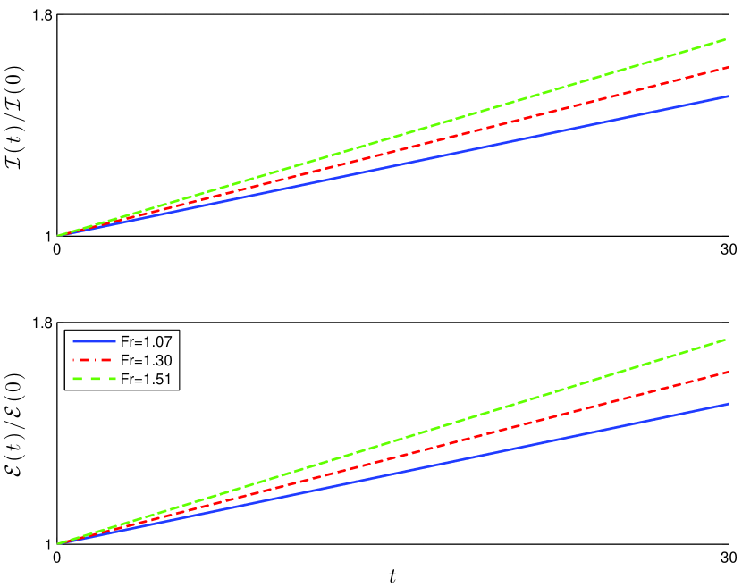
Figure 2. The momentum and the energy of the undular bore for $Fr=1.07$, $1.30$ and $1.51$.

In Figure 2, we present the normalized values $\mathcal{I}(t)/\mathcal{I}(0)$ of the momentum and $\mathcal{E}(t)/\mathcal{E}(0)$ of the total energy for the values of the Froude number $Fr=1.07$, $1.30$ and $1.51$. The slopes of the lines can be found in Tables 1 and 2.

Figure 3 shows the profiles of the undular bores generated when $h_{1}/h_{0}=1.3$, $1.5$ and $1.7$. From these figures we observe that as the Froude number $Fr$ increases, the peak amplitude of the leading wave becomes larger, and the shape of the wave envelope is changing. For example the shape of the wave envelope of Figure 3 (a) can be described by a quadratic function (wineglass shape) while the shape of the wave envelope of Figure 3 (c) can be described by a square-root function (martini glass shape). For the various shapes of the undular bores we refer to [51].

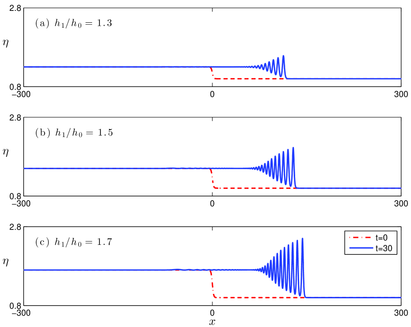
Figure 3. Undular bores profiles for various $Fr$ values.

4.2. Shoaling of solitary waves

In this section we study the conservation of energy in the case of a nonuniform bathymetry. Specifically, we consider the experiments proposed in [52, 53] related to the shoaling of solitary waves on a beach of slope $1:35$. The shoaling of solitary waves has been studied theoretically and experimentally in many works, such as in [52, 53, 54, 55]. Next, we study the shoaling of solitary waves with normalized amplitude $A=0.1$, $0.15$, $0.2$ and $0.25$ in the domain $[-100,34]$. In the numerical experiments we take $\Delta x=0.05$ while we translate the solitary waves such that the peak amplitude is achieved at $x=-20.1171$ while the bottom is described by the function

$$b(x)=\left\{\begin{array}[]{ll}-1,&x\leq 0\\ -1+x/35,&x>0\end{array}\right.\ ,$$

but modified appropriately around $x=0$ so as to be smooth enough and to satisfy the regularity requirements of the model.

A comparison between the experimental results on shoaling waves from [52], and the shoaling solitary waves computed with numerically approximation of (1) and (64) is presented in Figure 4. Overall, we observe a very good agreement between the numerical results and the experimental data.

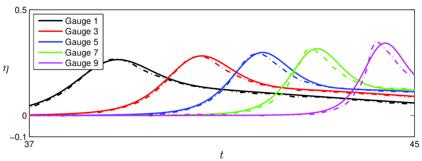
Figure 4. Comparison of the numerical solution and the experimental data on wave gauges of [53]. —-: Numerical solution; $-\cdot-$: Experimental data.

Table 3 presents the conserved values of the total energy $\mathcal{E}$ and of the Hamiltonian $\mathcal{H}$ for $t\in[0,45]$ for the computations shown in Figure 4. We observe that the energy is conserved with more than ten decimal digits. Due to the small values of $\Delta x$ and $\Delta t$ no energy dissipation can be observed verifying the efficacy of the numerical method.

Table 3. Conserved values of energy (in Joules) and Hamiltonian for shoaling of solitary waves on a plane beach of slope $1:35$.

$A$	$\mathcal{E}$	$\mathcal{H}$
$0.10$	$62.4704607870$	$0.05202930490$
$0.15$	$62.7102258381$	$0.09856973753$
$0.20$	$62.9401348199$	$0.15627417412$
$0.25$	$63.1680884219$	$0.22460417742$

Although the total energy is conserved the kinetic and the potential energy are not constant with time. Figure 5 presents the normalized kinetic energy $\mathcal{E}_{k}(t)/\mathcal{E}_{k}(0)$ and normalized potential energy $\mathcal{E}_{p}(t)/\mathcal{E}_{p}(0)$ evaluated in the spatial interval $[-100,34]$. As can be seen in Figure 5 the kinetic energy is decreasing at the early stages of shoaling due to the slight decrease in the wave speed while the potential energy is initially increasing due to the increase of the wave height. At later stages of the shoaling, the kinetic energy increases again, due to the increase in particle velocities, and the potential energy decreases again, due to the rising bottom, and narrowing wave peak. Nevertheless, the total energy is constant over time.

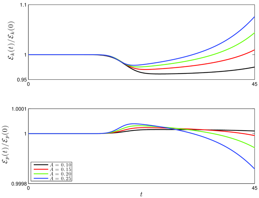
Figure 5. Normalized Kinetic and Potential energy for shoaling of solitary waves on a plane beach of slope $1:35$.

5. Summary and Conclusions

We have detailed the derivation of mechanical balance laws for the SGN equations in the case of a horizontal bed and also in the case of varying bathymetry. The mechanical balance laws derived here, including the mass, momentum and energy balance laws, are valid to the same asymptotic order as the SGN system, providing a firm link between conservation laws associated to the governing SGN equations, and the above mechanical quantities. Finally, applications to the energy budget of undular bores and the development of potential and kinetic energy in shoaling solitary waves have been presented. In particular, it has been shown that the energy loss in undular bores is fully compensated for by the development of surface oscillations, since the energy in the SGN with a flat bottom is exactly conserved. Indeed, exact conservation of energy to near machine precision was observed in our numerical computations, and this gave an additional check on the implementation of the numerical algorithm.

Appendix A The numerical method

In this Appendix we consider the initial-boundary value problem (IBVP) comprised of system (28a)–(28b) subject to reflective boundary conditions. Rewriting the system in terms of $(h,\ u)$, and dropping the bar over the symbol of the horizontal velocity, yields the IBVP

$$\begin{array}[]{l}h_{t}+(hu)_{x}=0\ ,\\ hu_{t}+huu_{x}+g(h+b)_{x}+\\ \left[h^{2}\big{(}{\textstyle\frac{1}{3}}\mathcal{P}+{\textstyle\frac{1}{2}}\mathcal{Q}\big{)}\right]_{x}+b_{x}\big{(}{\textstyle\frac{1}{2}}\mathcal{P}+\mathcal{Q}\big{)}=0\ ,\\ u(a,t)=u(b,t)=0\ ,\\ h(x,0)=h_{0}(x)\ ,\\ u(x,0)=u_{0}(x)\ ,\end{array}$$ (64)

where $\mathcal{P}=h\left[u_{x}^{2}-u_{xt}-uu_{xx}\right]$, $\mathcal{Q}=b_{x}(u_{t}+uu_{x})+b_{xx}u^{2}$, $x\in[a,\ b]\subset\mathbb{R}$ and $t\in[0,\ T]$. Considering a spatial grid $x_{i}=a+i\ \Delta x$, for $i=0,1,\cdots,N$, where $\Delta x$ is the spatial mesh-length, such that $\Delta x=(b-a)/N$, $N\in\mathbb{N}$. We define the space of cubic splines

$$S=\left\{\phi\in C^{2}[a,b]\Big{|}\phi|_{[x_{i},x_{i+1}]}\in\mathbb{P}^{3},\ 0\leq i\leq N-1\right\}\ ,$$

where $\mathbb{P}^{k}$ is the space of polynomials of degree $k$. We also consider the space

$$S_{0}=S\cap\left\{\phi\in C([a,b])\Big{|}\phi(a)=\phi(b)=0\right\}\ .$$

The basis functions of the space $S$ and $S_{0}$ consist of the usual B-splines described in [56].

$N$	$E_{0}[H]$	rate for $E_{0}[H]$	$E_{0}[U]$	rate for $E_{0}[U]$
$300$	$0.1211\times 10^{-8}$	–	$0.6127\times 10^{-11}$	–
$320$	$0.9674\times 10^{-9}$	$3.4793$	$0.4733\times 10^{-11}$	$3.9983$
$340$	$0.7836\times 10^{-9}$	$3.4772$	$0.3714\times 10^{-11}$	$3.9999$
$360$	$0.6422\times 10^{-9}$	$3.4797$	$0.2955\times 10^{-11}$	$3.9977$
$380$	$0.5322\times 10^{-9}$	$3.4754$	$0.2382\times 10^{-11}$	$3.9885$
$400$	$0.4452\times 10^{-9}$	$3.4793$	$0.1939\times 10^{-11}$	$4.0099$

Table 4. Spatial errors and rates of convergence in the $L^{2}$ norm.

The semi-discrete scheme is reduced in finding $\tilde{h}\in S$ and $\tilde{u}\in S_{0}$ such that

$$\begin{array}[]{l}(\tilde{h}_{t},\phi)+\left((\tilde{h}\tilde{u})_{x},\phi\right)=0\ ,\\ \mathcal{B}(\tilde{u}_{t},\psi;\tilde{h})+\left(\tilde{h}\tilde{u}\tilde{u}_{x}+g(\tilde{h}+b)_{x},\psi\right)+\\ +\left(\tilde{h}^{2}\big{(}{\textstyle\frac{1}{3}}\tilde{\mathcal{P}}+{\textstyle\frac{1}{2}}\tilde{\mathcal{Q}}\big{)},\psi_{x}\right)+\left(b_{x}({\textstyle\frac{1}{2}}\tilde{\mathcal{P}}+\tilde{\mathcal{Q}}),\psi\right)=0\ ,\end{array}$$ (65)

for $\phi\in S$, and $\psi\in S_{0}$, and $\tilde{\mathcal{P}}=\tilde{h}\left[\tilde{u}_{x}^{2}-\tilde{u}\tilde{u}_{xx}\right]$ and $\tilde{\mathcal{Q}}=b_{x}\tilde{u}\tilde{u}_{x}+b_{xx}\tilde{u}^{2}$. $\mathcal{B}$ is defined as the bilinear form that for fixed $\tilde{h}$ is given by

$$\mathcal{B}(\psi,\chi;\tilde{h})=\left(\tilde{h}\left[1+\tilde{h}_{x}b_{x}+\frac{1}{2}\tilde{h}b_{xx}+b_{x}^{2}\right]\psi,\chi\right)+\\ +{\textstyle{1\over 3}}\left(\tilde{h}^{3}\psi_{x},\chi_{x}\right)\ \mbox{for }\psi,\chi\in S_{0}\ .$$ (66)

The system of equations (65) is accompanied by the initial conditions

$$\tilde{h}(x,0)=\mathcal{P}\{h_{0}(x)\}\ ,\quad\tilde{u}(x,0)=\mathcal{P}_{0}\{u_{0}(x)\}\ ,$$ (67)

where $\mathcal{P}$ and $\mathcal{P}_{0}$ are the $L^{2}$-projections onto $S$ and $S_{0}$ respectively, satisfying $(\mathcal{P}v,\phi)=(v,\phi)$ for all $\phi\in S$ and $(\mathcal{P}_{0}v,\psi)=(v,\psi)$ for all $\psi\in S_{0}$. Upon choosing basis functions $\phi_{j}$ and $\psi_{j}$ for the spaces $S$ and $S_{0}$, (65) is reduced to a system of ordinary differential equations (ODEs). For the integration in time of this system we employ the Dormand–Prince adaptive time-stepping methods, [57, 58]. One may apply the same numerical method to solve the IBVP with non-homogeneous Dirichlet boundary conditions. For example if $u(a,t)=u_{a}$ then the change of variables $u(x,t)=w(x,t)+u_{0}(x)$ reduces the non-homogeneous system to a homogeneous IBVP system for the variable $w$. In all the numerical experiments we took $\Delta x=0.1$, while the tolerance for the relative error of the adaptive Runge–Kutta scheme was taken $5\cdot 10^{-14}$. For the computations of the integrals the Gauss-Legendre quadrature rule with $8$ nodes was employed.

The convergence properties of the standard Galerkin method for the SGN system are very similar with those of the classical Boussinesq system studied in detail in [59, 60]. In order to compute the convergence rates in various norms we consider the nonhomogeneous SGN system with flat bottom admitting the exact solution $h(x,t)=1+e^{2t}(\cos(\pi x)+x+2)$ and $u(x,t)=e^{-tx}x\sin(\pi x)$ for $0\leq x\leq 1$, and for $t\in(0,T]$ with $T=1$. We compute the normalized errors

$$E_{s}[F]\doteq\frac{\|F(x,T;\Delta x)-F_{\mbox{exact}}(x,T)\|_{s}}{\|F_{\mbox{exact}}(x,T)\|_{s}}\ ,$$ (68)

where $F=F(\cdot;\Delta x)$ is the computed solution, i.e., either $H\approx h(x,T)$ or $U\approx u(x,T)$, $F_{\mbox{exact}}$ is the corresponding exact solution and $s=0,1,2,\infty$ correspond to the $L^{2}$, $H^{1}$, $H^{2}$ and $L^{\infty}$ norms, respectively. The analogous rates of convergence are defined as

$$\mbox{rate for }E_{s}[F]\doteq\frac{\ln(E_{s}[F(\cdot;\Delta x_{k-1})]/E_{s}[F(\cdot;\Delta x_{k})])}{\ln(\Delta x_{k-1}/\Delta x_{k})}\ ,$$ (69)

where $\Delta x_{k}$ is the grid size listed in row $k$ in table 4. To ensure that the errors incurred by the temporal integration do not affect the rates of convergence we use $\Delta t\ll\Delta x$ while we take $\Delta x=1/N$.

Table 4 presents the spatial convergence rates in the $L^{2}$ norm. We observe that the convergence is optimal for the $u$ variable but suboptimal for the $h$ variable. Specifically, it appears that $\|h-\tilde{h}\|\sim\Delta x^{3.5}$, while $\|u-\tilde{u}\|\sim\Delta x^{4}$. More precisely, as in the case of the classical Boussinesq system [59], and because the rate of convergence in $h$ appears to be less that $3.5$ yields that the error should be of $O(\Delta x^{3.5}\sqrt{\ln(1/\Delta x)})$. Similar results obtained for the convergence in the $H^{1}$, $H^{2}$ and $L^{\infty}$ norms. Specifically it was observed numerically that $\|h-\tilde{h}\|_{s}\sim\Delta x^{3.5-s}$, $\|u-\tilde{u}\|_{1}\sim\Delta x^{4-s}$, for $s=0,1,2$ and $\|h-\tilde{h}\|_{\infty}\sim\Delta x^{3}$, while $\|u-\tilde{u}\|_{\infty}\sim\Delta x^{4}$ approximately.

References

- [1] F. Serre, Contribution á l’ étude des écoulements permanents et variables dans les canaux, Houille Blanche 8 (1953) 374–388.
- [2] F. Serre, Contribution á l’ étude des écoulements permanents et variables dans les canaux, Houille Blanche 8 (1953) 830–872.
- [3] C. H. Su, C. S. Gardner, Korteweg-de Vries equation and generalizations. III. Derivation of the Korteweg-de Vries equation and Burgers equation., J. Math. Phys. 10 (1969) 536–539.
- [4] A. Green, P. Naghdi, A derivation of equations for wave propagation in water of variable depth, J. Fluid Mech. 78 (1976) 237–246.
- [5] F. Seabra-Santos, D. Renouard, A. Temperville, Numerical and experimental study of the transformation of a solitary wave over a shelf or isolated obstacle, J. Fluid Mech. 176 (1987) 117–134.
- [6] D. Lannes, P. Bonneton, Derivation of asymptotic two-dimensional time-dependent equations for surface water wave propagation, Physics of Fluids 21 (2009) 016601.
- [7] D. Lannes, The water waves problem: Mathematical analysis and asymptotics, American Mathematical Society, 2013.
- [8] E. Barthelemy, Nonlinear shallow water theories for coastal waves, Surv. Geophys. 25 (2004) 315–337.
- [9] G. Wei, J. T. Kirby, S. T. Grilli, R. Subramanya, A fully nonlinear boussinesq model for surface waves. part 1. highly nonlinear unsteady waves, Journal of Fluid Mechanics 294 (1995) 71–92.
- [10] P. A. Madsen, D. R. Fuhrman, B. Wang, A boussinesq-type method for fully nonlinear waves interacting with a rapidly varying bathymetry, Coastal Engineering 53 (5) (2006) 487–504.
- [11] M. Brocchini, A reasoned overview on Boussinesq-type models: the interplay between physics, mathematics and numerics, Proc. R. Soc. A 469 (0496) (2013) 1–27.
- [12] J. Carter, R. Cienfuegos, The kinematics and stability of solitary and cnoidal wave solutions of the Serre equations, European Journal of Mechanics B: Fluids 30 (2011) 259–268.
- [13] S. Gavrilyuk, H. Kalisch, Z. Khorsand, A kinematic conservation law in free surface flow, Nonlinearity 28 (6) (2015) 1805–1821.
- [14] G. Whitham, Variational methods and applications to water waves, Proc. R. Soc. Lond., Ser. A 299 (1967) 6–25.
- [15] M. Ehrnström, H. Kalisch, Traveling waves for the Whitham equation, Differential Integral Equations 22 (11-12) (2009) 1193–1210.
- [16] R. Cienfuegos, E. Barthelemy, P. Bonneton, A fourth-order compact finite volume scheme for fully nonlinear and weakly dispersive Boussinesq-type equations. Part I: Model development and analysis, Int. J. Numer. Meth. Fluids 51 (2006) 1217–1253.
- [17] D. Peregrine, Long waves on beaches, J. Fluid Mech. 27 (1967) 815–827.
- [18] Y. Li, Linear stability of solitary waves of the Green-Naghdi equations, Comm. Pure Appl. Math. 54 (2001) 501–536.
- [19] Y. Li, Hamiltonian structure and linear stability of solitary waves of the Green-Naghdi equations, J. Nonlin. Math. Phys. 9 (2002) 99–105.
- [20] D. Mitsotakis, J. Carter, D. Dutykh, On the nonlinear dynamics of the traveling wave solutions of the serre equations, Preprint.
- [21] Z. Khorsand, Particle trajectories in the Serre equations, Appl. Math. Comp. 230 (0496) (2014) 35–42.
- [22] R. Camassa, D. Holm, C. Levermore, Long-time effects of bottom topography in shallow water, Physica D 98 (2) (1996) 258–286.
- [23] R. S. Johnson, Camassa-Holm, Korteweg-de Vries and related models for water waves, J. Fluid Mech. 455 (2002) 63–82.
- [24] S. Israwi, Large time existence for 1D Green-Naghdi equations, Nonlinear Analysis 74 (81–93).
- [25] H. Kalisch, Mechanical balance laws in long wave models, Oberwolfach Reports - OWR 2015 (19) (2015) 28–31.
- [26] A. Ali, H. Kalisch, Mechanical balance laws for Boussinesq models of surface water waves, J. Nonlinear Sci. 22 (2012) 371–398.
- [27] A. Ali, H. Kalisch, On the formulation of mass, momentum and energy conservation in the KdV equation, Acta Appl. Math. 133 (1) (2014) 113–131.
- [28] Z. I. Fedotova, G. S. Khakimzyanov, and D. Dutykh. Energy equation for certain approximate models of long-wave hydrodynamics, Russ. J. Numer. Anal. Math. Modelling 29 (2014) 167–178.
- [29] L. Rayleigh, On the theory of long waves and bores, Proc. R. Soc. A 90 (1914) 324–328.
- [30] T. Benjamin, J. Lighthill, On cnoidal waves and bores, Proc. R. Soc. A 224 (1954) 448–460.
- [31] B. Sturtevant, Implications of experiments on the weak undular bore, Phys. Fluids 8 (1965) 1052–1055.
- [32] A. Ali, H. Kalisch, Energy balance for undular bores, C. R. Mecanique 338 (2010) 67–70.
- [33] A. Ali, H. Kalisch, A dispersive model for undular bores, Anal. Math. Phys. 2 (2012) 347–366.
- [34] D. Mitsotakis, B. Ilan, D. Dutykh, On the Galerkin / finite-element method for the Serre equations, J. Sci. Comp.
- [35] O. L. Métayer, S. Gavrilyuk, S. Hank, A numerical scheme for the Green-Naghdi model, Journal of Computational Physics 229 (6) (2010) 2034 – 2045.
- [36] D. Dutykh, D. Clamond, P. Milewski, D. Mitsotakis, Finite volume and pseudo-spectral schemes for the fully nonlinear 1D Serre equations, European J. Appl. Math. 24 (2013) 761–787.
- [37] P. Bonneton, F. Chazel, D. Lannes, F. Marche, M. Tissier, A splitting approach for the fully nonlinear and weakly dispersive Green-Naghdi model, J. Comput. Phys. 230 (2011) 1479–1498.
- [38] R. Cienfuegos, E. Barthelemy, P. Bonneton, A fourth-order compact finite volume scheme for fully nonlinear and weakly dispersive Boussinesq-type equations. Part II: Boundary conditions and model validation, Int. J. Numer. Meth. Fluids 53 (2007) 1423–1455.
- [39] G. El, R. Grimshaw, N. Smyth, Unsteady undular bores in fully nonlinear shallow-water theory, Phys. Fluids 18 (2006) 027104.
- [40] D. Mitsotakis, C. Synolakis, M. McGuinness, A Modified Galerkin / Finite Element Method for the numerical solution of the Serre-Green-Naghdi system, Submitted.
- [41] G. B. Whitham, Linear and nonlinear waves, John Wiley & Sons Inc., New York, 1999.
- [42] E. N. Pelinovsky, H. S. Choi, A mathematical model for non-linear waves due to moving disturbances in a basin of variable depth, J. Korean Soc. Coastal Ocean Eng. 5 (1993) 191–197.
- [43] H. Favre, Ondes de translation, Dunond, Paris, 1935.
- [44] H. Chanson, Current knowledge in hydraulic jumps and related phenomena: A survay of experimental results, Eur. J. Mech. B/Fluids 28 (2) (2009) 191–210.
- [45] M. Tissier, P. Bonneton, F. Marche, F. Chazel, D. Lannes, Nearshore Dynamics of Tsunami-like Undular Bores using a fully-nonlinear Boussinesq Model, Journal of Coastal Research 64 (2011) 603–607.
- [46] M. Tissier, P. Bonneton, F. Marche, F. Chazel, D. Lannes, A new approach to handle wave breaking in fully non-linear Boussinesq models, Coastal Engineering 67 (2012) 54–66.
- [47] G. Richard, S. Gavrilyuk, The classical hydraulic jump in a model of shear shallow-water flows, J. Fluid Mech. 725 (2013) 492–521.
- [48] G. B. Whitham, A general approach to linear and non-linear dispersive waves using a Lagrangian, J. Fluid Mech. 22 (1965) 273–283.
- [49] R. Grimshaw, Solitary waves in fluids, Advances in Fluid Mechanics 47 (2007) 208pp.
- [50] M. Bestehorn, P. Tyvand, Merging and colliding bores, Phys. Fluids 21 (042107) (2009) 1–11.
- [51] M. Hoefer, Shock waves in dispersive Eulerian fluids, J. Nonlinear Sci. 24 (525–577).
- [52] S. Grilli, R. Subramanya, I. Svendsen, J. Veeramony, Shoaling of solitary waves on plane beaches, J. Waterway, Port, Coastal, and Ocean Eng. 120 (1994) 609–628.
- [53] S. Grilli, I. Svendsen, R. Subramanya, Breaking criterion and characteristics for solitary waves on slopes, J. Waterway, Port, Coastal, and Ocean Eng. 123 (1997) 102–112.
- [54] C. Synolakis, Green’s law and the evolution of solitary waves, Phys. Fluids 3 (1991) 490–491.
- [55] C. Synolakis, J. Skjelbreia, Evolution of maximum amplitude of solitary waves on plane beaches, J. Waterway, Port, Coastal, and Ocean Eng. 119 (1993) 323–342.
- [56] M. H. Schultz, Spline Analysis, 1st Edition, Prentice Hall, 1973.
- [57] J. Butcher, Numerical methods for ordinary differential equations, John Wiley and Sons Ltd, 2008.
- [58] E. Hairer, S. P. Nørsett, G. Wanner, Solving ordinary differential equations: Nonstiff problems, Springer, 2009.
- [59] D. Antonopoulos, V. Dougalis, Numerical solution of the ‘classical’ Boussinesq system, Math. Comp. Simul. 82 (2012) 984–1007.
- [60] D. Antonopoulos, V. Dougalis, Error estimates for Galerkin approximations of the “classical” Boussinesq system, Math. Comp. 82 (2013) 689–717.