Roles of Antinucleon Degrees of Freedom in the
Relativistic Random Phase Approximation

Haruki Kurasawa¹ and Toshio Suzuki²

¹  Department of Physics, Graduate School of Science, Chiba University, Chiba 263-8522, Japan

² Emeritus Professor, University of Fukui, Fukui 910-8507, Japan

Roles of antinucleon degrees of freedom in the relativistic random phase approximation(RPA) are investigated. The energy-weighted sum of the RPA transition strengths is expressed in terms of the double commutator between the excitation operator and the Hamiltonian, as in nonrelativistic models. The commutator, however, should not be calculated with a usual way in the local field theory, because, otherwise, the sum vanishes. The sum value obtained correctly from the commutator is infinite, owing to the Dirac sea. Most of the previous calculations takes into account only a part of the nucleon-antinucleon states, in order to avoid the divergence problems. As a result, RPA states with negative excitation energy appear, which make the sum value vanish. Moreover, disregarding the divergence changes the sign of nuclear interactions in the RPA equation which describes the coupling of the nucleon particle-hole states with the nucleon-antinucleon states. Indeed, excitation energies of the spurious state and giant monopole states in the no-sea approximation are dominated by those unphysical changes. The baryon current conservation can be described without touching the divergence problems. A schematic model with separable interactions is presented, which makes the structure of the relativistic RPA transparent.

1 Introduction

It has been shown by many authors[1, 2, 3, 4] that relativistic models, assuming nuclei to be composed of Dirac particles and various mesons, work well phenomenologically to reproduce nuclear static and dynamic properties. In most of calculations, however, antinucleon($\mathrm{\overline{N}}$) degrees of freedom are not fully taken into account, in spite of the fact that they are one of the main differences between relativistic and non-relativistic models. The reason why the full space is not used is because there exist divergence problems[1, 5, 6] which are not yet handled with a proper way for finite nuclei.

Although all the space was not included in the previous calculations, a part of $\mathrm{\overline{N}}$ degrees of freedom was taken into account, aiming to keep some fundamental principles and to reproduce gross properties of nuclei.

For example, in the random phase approximation (RPA), the baryon current conservation required some excitations of antinucleons[5, 6, 7]. It was necessary for description of the center of mass motion to have the Landau-Migdal parameter $F_{1}$ taking into account a part of N(nucleon)-$\mathrm{\overline{N}}$ states[7, 8]. In the same way, the spurious states in RPA[9, 10] was described with those N-$\mathrm{\overline{N}}$ excitations in addition to nucleon particle-hole states. Furthermore, an abnormal enhancement of the isoscalar magnetic moment in the Hartree approximation demanded corrections from the N-$\mathrm{\overline{N}}$ excitations through $F_{1}$ [11].

For the above reasons, the two ways to include the $\mathrm{\overline{N}}$ space, avoiding the divergence problem, were proposed. The one is the no free term approximation(NFA) which simply neglects the divergent part of the RPA response functions. The remaining part is composed of transitions of antinucleons to the Fermi sea which are in fact Pauli-blocked[5, 6]. The other is the no-sea approximation(NSA) to assume that all the $\mathrm{\overline{N}}$ states are empty. There is no divergence problem in this case also, but transitions of nucleons in the Fermi sea to the $\mathrm{\overline{N}}$ states are permitted with negative excitation energies[10]. Even though both methods look unreasonable, they have been widely used, since experimental data are well reproduced phenomenologically[3, 12, 13, 14]. In fact, as will be seen later explicitly, NFA and NSA are equivalent to each other in RPA[10].

The purpose of the present paper is to investigate the structure of the relativistic RPA in detail, and in particular, a role of $\mathrm{\overline{N}}$ degrees of freedom there. The relativistic RPA can be developed almost in the same way as non-relativistic ones. It will be shown, however, that a careful treatment is required for $\mathrm{\overline{N}}$ degrees of freedom. They cause the divergence problems, but cannot be simply ignored as in NFA and NSA.

It will be shown that the energy-weighted sum of the RPA transition strengths is expressed formally in terms of the double commutator between the transition operator and the Hamiltonian. This RPA sum rule is the same as in nonrelativistic case. The commutator, however, should not be calculated employing a usual rule in the local field theory. Otherwise, the sum vanishes, in spite of the fact that it should be positive definite. The correct calculation of the commutator gives the sum value to be infinite, because of N-$\mathrm{\overline{N}}$ excitations.

In NFA and NSA, RPA states with negative excitation-energy appear, in addition to those with positive energy. This is due to the fact that the full N-$\mathrm{\overline{N}}$ excitations are not take into account. As a result, the energy-weighted sum value of the excitation strengths vanishes. Moreover, disregard of the divergence in NSA and NFA gives rise to other unphysical results. The sign of the nuclear interactions is changed in RPA equation relevant to the remaining N-$\mathrm{\overline{N}}$ states. Because of this fact, attractive (repulsive) forces work as repulsive (attractive) ones in the coupling of nucleon particle-hole states with N-$\mathrm{\overline{N}}$ states considered in NFA and NSA. These effects are not negligible, but dominate the excitation energies of some low lying states. For example, the previous numerical calculations could reproduce a spurious state[9, 10] and giant monopole states[12, 13, 14], invoking those unphysical effects hidden in the RPA equation.

The above defects of NFA and NSA have not been investigated explicitly so far, since the structure of the relativistic RPA formulae may be rather complicated, compared with non-relativistic ones. In the next section, we will briefly review the relativistic RPA focusing on roles of N-$\mathrm{\overline{N}}$ states in various approximations. In §3, the energy-weighted sum of the RPA excitation strengths is discussed, according to recent new insight for the long-standing problem on the relativistic sum rule[15]. In §4 and §5, we will explore in detail why NFA and NSA seemed to describe well the continuity equation and the spurious state without the full N-$\mathrm{\overline{N}}$ excitations.

It is well-known that a schematic model with separable interactions helps us to understand the structure of nonrelativistic RPA[16]. In §6, a similar model will be introduced for the relativistic RPA, in order to make clear the present discussions. The final section is devoted to a brief summary of the present paper.

2 Relativistic RPA

The relativistic RPA was formulated in various ways[1, 5, 6, 9, 10]. Taking notice of the dependence on N-$\mathrm{\overline{N}}$ states, let us briefly review it.

We begin with the Hartree polarization function for arbitrary $4\times 4$ matrices, $A$ and $B$ [6],

$$i\varPi_{\mathrm{H}}(A(1),B(2))=\langle\,\!\ \,|\,\mathrm{T}\Bigl{(}\overline{\psi}(1)A\psi(1)\,\overline{\psi}(2)B\psi(2)\Bigr{)}\,|\,\!\ \,\rangle,$$ (1)

defined for the Hartree ground state $|\,\!\ \,\rangle$. The baryon field $\psi(x)$ is written using the complete set of the eigenfunction, $\varphi_{\alpha}$, of Hartree Hamiltonian,

$$\psi(x)=\sum_{\alpha}\varphi_{\alpha}(\boldsymbol{x})e^{-iE_{\alpha}t}a_{\alpha},$$ (2)

where $E_{\alpha}$ denotes the eigenvalue of $\varphi_{\alpha}$, and $a_{\alpha}$ plays a role of the annihilation or creation operator of N and $\mathrm{\overline{N}}$, satisfying $\{\,a_{\alpha}\,,\,a_{\beta}^{\dagger}\,\}=\delta_{\alpha\beta}$, etc.. Then, together with the closure property of $\varphi_{\alpha}$,

$$\sum_{\alpha}\varphi_{\alpha}(\boldsymbol{x})\varphi^{\dagger}_{\alpha}(\boldsymbol{x}^{\prime})=\delta(\boldsymbol{x}-\boldsymbol{x}^{\prime}),$$ (3)

the baryon field satisfies the anti-commutation relation,

$$\{\,\psi_{a}(x_{0},\boldsymbol{x})\,,\,\psi_{b}^{\dagger}(x_{0},\boldsymbol{x}^{\prime})\,\}=\delta_{ab}\,\delta(\boldsymbol{x}-\boldsymbol{x}^{\prime}),$$ (4)

where $a$ and $b$ denote the Dirac matrix indices. Since the simple interactions have rather advantage for our purpose to investigate the detail of the relativistic RPA structure, we assume, throughout the present paper, the $\sigma$-$\omega$ model[1], which provides us with the Hartree Hamiltonian as

$$h(x)=-\,i\boldsymbol{\alpha}\!\cdot\!\boldsymbol{\nabla}+\gamma_{0}M+V_{\mathrm{H}}(x)\,,\quad V_{\mathrm{H}}(x)=\gamma_{0}\varSigma(x).$$ (5)

In the above equation, we have employed the following abbreviation for the potential,

$$\varSigma(x)=V_{\sigma}(x)+\gamma^{\mu}V_{\mu}(x)$$ (6)

with

$$V_{\sigma}(x) =g_{\sigma}^{2}\int\!\mathrm{d}^{4}y\,D_{\sigma}(x-y)\,\langle\,\!\ \,|\,\overline{\psi}(y)\psi(y)\,|\,\!\ \,\rangle,$$ (7)

$$V_{\mu}(x) =g_{\omega}^{2}\int\!\mathrm{d}^{4}y\,D_{\omega}(x-y)\,\langle\,\!\ \,|\,\overline{\psi}(y)\gamma_{\mu}\psi(y)\,|\,\!\ \,\rangle,$$ (8)

$g_{\sigma}$ and $g_{\omega}$ being the coupling constants, and $D_{\sigma}$ and $D_{\omega}$ denoting the $\sigma$- and $\omega$-meson propagators, respectively[6],

$$D_{\sigma}(x) =\int\!\frac{\mathrm{d}k_{0}}{2\pi}e^{-ik_{0}x_{0}}D_{\sigma}(k_{0},\boldsymbol{x}),\quad D_{\sigma}(k_{0},\boldsymbol{x})=\int\!\frac{\mathrm{d}^{3}k}{(2\pi)^{3}}\,\frac{e^{i\boldsymbol{k}\cdot\boldsymbol{x}}}{k_{\mu}k^{\mu}-m_{\sigma}^{2}+i\varepsilon},$$ (9)

$$D_{\omega}(x) =\int\!\frac{\mathrm{d}k_{0}}{2\pi}e^{-ik_{0}x_{0}}D_{\omega}(k_{0},\boldsymbol{x}),\quad D_{\omega}(k_{0},\boldsymbol{x})=-\int\!\frac{\mathrm{d}^{3}k}{(2\pi)^{3}}\,\frac{e^{i\boldsymbol{k}\cdot\boldsymbol{x}}}{k_{\mu}k^{\mu}-m_{\omega}^{2}+i\varepsilon}.$$ (10)

Here, $m_{\sigma}$ and $m_{\omega}$ represent the masses of the $\sigma$- and $\omega$-mesons.

The calculation of Eq.(1) gives[6],

$$\varPi_{\mathrm{H}}(A(1),B(2))=\frac{1}{2\pi}\int\!\mathrm{d}\omega\,e^{-i\omega(t_{1}-t_{2})}\varPi_{\mathrm{H}}(A(\boldsymbol{x}_{1}),B(\boldsymbol{x}_{2}),\omega),$$ (11)

where we have defined

$$\varPi_{\mathrm{H}}(A(\boldsymbol{x}_{1}),B(\boldsymbol{x}_{2}),\omega)=\sum_{\alpha\beta}\overline{\varphi}_{\beta}(\boldsymbol{x}_{1})A\varphi_{\alpha}(\boldsymbol{x}_{1})\,\overline{\varphi}_{\alpha}(\boldsymbol{x}_{2})B\varphi_{\beta}(\boldsymbol{x}_{2})\,(\varPi_{\mathrm{H}})_{\alpha\beta}(\omega)$$ (12)

with

$$(\varPi_{\mathrm{H}})_{\alpha\beta}(\omega)=\frac{N_{\alpha\beta}}{\omega-E_{\alpha\beta}+i\varepsilon}-\frac{N_{\beta\alpha}}{\omega-E_{\alpha\beta}-i\varepsilon}\,,\qquad N_{\alpha\beta}=\left(1-\theta_{\alpha}\right)\theta_{\beta}.$$ (13)

In this equation, $E_{\alpha\beta}$ stands for the excitation energy, $E_{\alpha}-E_{\beta}$, and $N_{\alpha\beta}$ implies the transition from the occupied state to unoccupied state as,

$$\theta_{\alpha}=\left\{\begin{array}[]{ll}1\,,&\alpha\,:\,\mbox{occupied state in }|\,\!\ \,\rangle,\\[2.0pt] 0\,,&\alpha\,:\,\mbox{unoccupied state in }|\,\!\ \,\rangle.\end{array}\right.$$ (14)

Defining the Fermi energy by $E_{\mathrm{F}}$, it is convenient to employ the following notations for $N_{\alpha\beta}$,

$$p_{\alpha}=\theta(E_{\alpha}-E_{\mathrm{F}})\,,\qquad h_{\alpha}=\theta(E_{\alpha})\,\theta(E_{\mathrm{F}}-E_{\alpha})\,,\qquad\bar{n}_{\alpha}=\theta(-E_{\alpha}),$$ (15)

where $p_{\alpha}$, $h_{\alpha}$, and $\bar{n}_{\alpha}$ indicate the particle, hole and $\mathrm{\overline{N}}$ states, respectively. In the full space calculation, the occupied states are expressed by ($h+\bar{n}$), and unoccupied states by $p$, so that $N_{\alpha\beta}$ is written as $N_{\alpha\beta}=p_{\alpha}(h_{\beta}+\bar{n}_{\beta})$. In NSA where the $\mathrm{\overline{N}}$ states are empty, we have $N_{\alpha\beta}=(p_{\alpha}+\bar{n}_{\alpha})h_{\beta}$. In writing $N_{\alpha\beta}=p_{\alpha}h_{\beta}-h_{\alpha}\bar{n}_{\beta}+(p_{\alpha}+h_{\alpha})\bar{n}_{\beta}$ for the full space, NFA neglects the last term which describes the vacuum polarization to produce the divergence[5, 6]. In the approximation neglecting all the $\mathrm{\overline{N}}$ states(No$\mathrm{\overline{N}}$), $N_{\alpha\beta}$ is simply given by $p_{\alpha}h_{\beta}$. Thus, the difference between various approximations can be represented by $N_{\alpha\beta}$, reading it as

$$N_{\alpha\beta}=\left\{\begin{array}[]{ll}p_{\alpha}h_{\beta}+p_{\alpha}\bar{n}_{\beta}&(\mbox{Full}),\\[2.0pt] p_{\alpha}h_{\beta}+\bar{n}_{\alpha}h_{\beta}&\mbox{(NSA)},\\[2.0pt] p_{\alpha}h_{\beta}-h_{\alpha}\bar{n}_{\beta}&\mbox{(NFA)},\\[2.0pt] p_{\alpha}h_{\beta}&(\mathrm{No}\mathrm{\overline{N}})\,.\end{array}\right.$$ (16)

We define the inverse of $\varPi_{\mathrm{H}}$ by $\varPi_{\mathrm{H}}^{-1}$ as

$$\sum_{\alpha^{\prime\prime}\beta^{\prime\prime}}(\varPi_{\mathrm{H}}^{-1})_{\alpha\beta,\alpha^{\prime\prime}\beta^{\prime\prime}}(\varPi_{\mathrm{H}})_{\alpha^{\prime\prime}\beta^{\prime\prime},\alpha^{\prime}\beta^{\prime}}=I_{\alpha\beta,\alpha^{\prime}\beta^{\prime}},$$

where the following abbreviations are used

$$(\varPi_{\mathrm{H}})_{\alpha\beta,\alpha^{\prime}\beta^{\prime}}=\delta_{\alpha\alpha^{\prime}}\delta_{\beta\beta^{\prime}}(\varPi_{\mathrm{H}})_{\alpha\beta}\,,\qquad I_{\alpha\beta,\alpha^{\prime}\beta^{\prime}}=\delta_{\alpha\alpha^{\prime}}\delta_{\beta\beta^{\prime}}\Bigl{(}N_{\alpha\beta}^{2}+N_{\beta\alpha}^{2}\Bigr{)}.$$

For $N_{\alpha\beta}^{2}+N_{\beta\alpha}^{2}=1$, we obtain

$$(\varPi_{\mathrm{H}}^{-1}(\omega))_{\alpha\beta,\alpha^{\prime}\beta^{\prime}}=\delta_{\alpha\alpha^{\prime}}\delta_{\beta\beta^{\prime}}\left(N_{\alpha\beta}-N_{\beta\alpha}\right)\left(\omega-E_{\alpha\beta}\right).$$ (17)

Because of $p_{\alpha}+h_{\alpha}+\bar{n}_{\alpha}=1$, the above ($N_{\alpha\beta}-N_{\beta\alpha}$) is given for each approximation as

$$N_{\alpha\beta}-N_{\beta\alpha}=\left\{\begin{array}[]{ll}(h_{\beta}+\bar{n}_{\beta})-(h_{\alpha}+\bar{n}_{\alpha})&\mbox{(Full),}\\[2.0pt] h_{\beta}-h_{\alpha}&\mbox{(NSA, NFA),}\\[2.0pt] p_{\alpha}h_{\beta}-p_{\beta}h_{\alpha}&(\mathrm{No}\mathrm{\overline{N}}).\end{array}\right.$$ (18)

Unlike $\varPi_{\mathrm{H}}$, the inverse $\varPi_{\mathrm{H}}^{-1}$ of NSA is the same as for NFA. This fact makes NSA and NFA are equivalent to each other in RPA, as seen later.

The RPA polarization function is written in terms of $\varPi_{\mathrm{H}}$[6],

$$\varPi(A(1),B(2)) =\varPi_{\mathrm{H}}(A(1),B(2))$$

$$\phantom{=}+g_{\eta}^{2}\int\!\mathrm{d}^{4}x\,\mathrm{d}^{4}y\,\varPi_{\mathrm{H}}(A(1),\varGamma^{\eta}(x))D_{\eta}(x-y)\varPi(\varGamma_{\eta}(y),B(2)),$$ (19)

where $\eta=-1$ for $\sigma$ and, hence, $\varGamma_{\eta}=1$ for $\eta=-1$, and $\gamma_{\mu}$ for $\eta=\mu$. As in $\varPi_{\mathrm{H}}$, we write Eq.(19) in the form:

$$\varPi(A(1),B(2))=\frac{1}{2\pi}\int\!\mathrm{d}\omega\,e^{-i\omega(t_{1}-t_{2})}\varPi(A(\boldsymbol{x}_{1}),B(\boldsymbol{x}_{2}),\omega),$$ (20)

with

$$\varPi(A(\boldsymbol{x}_{1}),B(\boldsymbol{x}_{2}),\omega) =\varPi_{\mathrm{H}}(A(\boldsymbol{x}_{1}),B(\boldsymbol{x}_{2}),\omega)$$

$$+g_{\eta}^{2}\!\int\!\mathrm{d}^{3}x\,\mathrm{d}^{3}y\,\varPi_{\mathrm{H}}(A(\boldsymbol{x}_{1}),\varGamma^{\eta}(\boldsymbol{x}),\omega)D_{\eta}(\omega,\boldsymbol{x}-\boldsymbol{y})\varPi(\varGamma_{\eta}(\boldsymbol{y}),B(\boldsymbol{x}_{2}),\omega).$$

The above $\varPi(A(\boldsymbol{x}_{1}),B(\boldsymbol{x}_{2}),\omega)$ is described as

$$\varPi(A(\boldsymbol{x}_{1}),B(\boldsymbol{x}_{2}),\omega)=\sum_{\alpha\beta\alpha^{\prime}\beta^{\prime}}\overline{\varphi}_{\beta}(\boldsymbol{x}_{1})A\varphi_{\alpha}(\boldsymbol{x}_{1})\,\varPi_{\alpha\beta,\alpha^{\prime}\beta^{\prime}}(\omega)\,\overline{\varphi}_{\alpha^{\prime}}(\boldsymbol{x}_{2})B\varphi_{\beta^{\prime}}(\boldsymbol{x}_{2}),$$ (21)

where we have defined

$$\varPi_{\alpha\beta,\alpha^{\prime}\beta^{\prime}}(\omega)=\delta_{\alpha\alpha^{\prime}}\delta_{\beta\beta^{\prime}}(\varPi_{\mathrm{H}})_{\alpha\beta}(\omega)+\sum_{\alpha^{\prime\prime}\beta^{\prime\prime}}(\varPi_{\mathrm{H}})_{\alpha\beta}(\omega)V_{\alpha\beta^{\prime\prime},\beta\alpha^{\prime\prime}}(\omega)\varPi_{\alpha^{\prime\prime}\beta^{\prime\prime},\alpha^{\prime}\beta^{\prime}}(\omega),$$ (22)

using the notation

$$V_{\alpha\beta^{\prime},\beta\alpha^{\prime}}(\omega)=g_{\eta}^{2}\int\!\mathrm{d}^{3}x_{1}\,\mathrm{d}^{3}x_{2}\,\overline{\varphi}_{\alpha}(\boldsymbol{x}_{1})\varGamma^{\eta}\varphi_{\beta}(\boldsymbol{x}_{1})D_{\eta}(\omega,\boldsymbol{x}_{1}-\boldsymbol{x}_{2})\,\overline{\varphi}_{\beta^{\prime}}(\boldsymbol{x}_{2})\varGamma_{\eta}\varphi_{\alpha^{\prime}}(\boldsymbol{x}_{2}).$$

This is also written as

$$V_{\alpha\beta^{\prime},\beta\alpha^{\prime}}(\omega)=\langle\,\alpha,\beta^{\prime}\,|\,\,\mathcal{V}_{12}(\omega)\,\,|\,\beta,\alpha^{\prime}\,\rangle,$$ (23)

with

$$\mathcal{V}_{12}(\omega)=g_{\eta}^{2}(\gamma_{0}\varGamma^{\eta})_{1}(\gamma_{0}\varGamma_{\eta})_{2}D_{\eta}(\omega,\boldsymbol{x}_{1}-\boldsymbol{x}_{2}).$$

In relativistic models, nuclear interactions contain $\omega$-dependence coming from Eqs.(9) and (10). For later discussions of the relativistic RPA, however, we have to neglect this retardation effect, as in nonrelativistic RPA. Fortunately, their contributions to the interactions have been shown to be negligible in Ref.[17], when $m_{\sigma},m_{\omega}>\omega$. Hence, from now on we will develop the RPA, assuming $\mathcal{V}_{12}(0)$.

Eq.(22) is formally described as follows,

$$\varPi(\omega)=\varPi_{\mathrm{H}}(\omega)+\varPi_{\mathrm{H}}(\omega)V\varPi(\omega)\,,\qquad(\varPi_{\mathrm{H}})_{\alpha\beta,\alpha^{\prime}\beta^{\prime}}(\omega)\equiv\delta_{\alpha\alpha^{\prime}}\delta_{\beta\beta^{\prime}}(\varPi_{\mathrm{H}})_{\alpha\beta}(\omega).$$ (24)

Then, the inverse of $\varPi(\omega)$ can be written as $\varPi^{-1}=\varPi_{\mathrm{H}}^{-1}-V$ with

$$(\varPi^{-1}(\omega))_{\alpha\beta,\alpha^{\prime}\beta^{\prime}}=\delta_{\alpha\alpha^{\prime}}\delta_{\beta\beta^{\prime}}\left(N_{\alpha\beta}-N_{\beta\alpha}\right)\left(\omega-E_{\alpha\beta}\right)-V_{\alpha\beta^{\prime},\beta\alpha^{\prime}}.$$ (25)

Now let us define the eigenvector $C^{(n)}_{\alpha\beta}$ of the above equation[18],

$$\varPi^{-1}(\omega_{n})\,C^{(n)}=0,$$

which is

$$\left(N_{\alpha\beta}-N_{\beta\alpha}\right)E_{\alpha\beta}C^{(n)}_{\alpha\beta}+\sum_{\alpha^{\prime}\beta^{\prime}}V_{\alpha\beta^{\prime},\beta\alpha^{\prime}}C^{(n)}_{\alpha^{\prime}\beta^{\prime}}=\left(N_{\alpha\beta}-N_{\beta\alpha}\right)\omega_{n}C^{(n)}_{\alpha\beta}.$$ (26)

In writing

$$C^{(n)}_{\alpha\beta}=N_{\alpha\beta}X^{(n)}_{\alpha\beta}+N_{\beta\alpha}Y^{(n)}_{\beta\alpha},$$ (27)

the coupled equations are obtained,

$$\begin{split}E_{\alpha\beta}X^{(n)}_{\alpha\beta}+\sum_{\alpha^{\prime}\beta^{\prime}}N_{\alpha^{\prime}\beta^{\prime}}\Bigl{(}V_{\alpha\beta^{\prime},\beta\alpha^{\prime}}X^{(n)}_{\alpha^{\prime}\beta^{\prime}}+V_{\alpha\alpha^{\prime},\beta\beta^{\prime}}Y^{(n)}_{\alpha^{\prime}\beta^{\prime}}\Bigr{)}&=\omega_{n}X^{(n)}_{\alpha\beta},\\ E_{\alpha\beta}Y^{(n)}_{\alpha\beta}+\sum_{\alpha^{\prime}\beta^{\prime}}N_{\alpha^{\prime}\beta^{\prime}}\Bigl{(}V_{\beta\alpha^{\prime},\alpha\beta^{\prime}}Y^{(n)}_{\alpha^{\prime}\beta^{\prime}}+V_{\beta\beta^{\prime},\alpha\alpha^{\prime}}X^{(n)}_{\alpha^{\prime}\beta^{\prime}}\Bigr{)}&=-\,\omega_{n}Y^{(n)}_{\alpha\beta}.\end{split}$$ (28)

Employing the abbreviations

$$\begin{split}A_{\alpha\beta,\alpha^{\prime}\beta^{\prime}}&=\delta_{\alpha\alpha^{\prime}}\delta_{\beta\beta^{\prime}}N_{\alpha\beta}E_{\alpha\beta}+N_{\alpha\beta}V_{\alpha\beta^{\prime},\beta\alpha^{\prime}}N_{\alpha^{\prime}\beta^{\prime}},\\ B_{\alpha\beta,\alpha^{\prime}\beta^{\prime}}&=N_{\alpha\beta}V_{\alpha\alpha^{\prime},\beta\beta^{\prime}}N_{\alpha^{\prime}\beta^{\prime}},\end{split}$$ (29)

Eq.(28) provides us with the relativistic RPA equation of the form:

$$\sum_{\alpha^{\prime}\beta^{\prime}}\left(\begin{array}[]{cc}A_{\alpha\beta,\alpha^{\prime}\beta^{\prime}}&B_{\alpha\beta,\alpha^{\prime}\beta^{\prime}}\\[4.0pt] B_{\alpha\beta,\alpha^{\prime}\beta^{\prime}}^{\ast}&A_{\alpha\beta,\alpha^{\prime}\beta^{\prime}}^{\ast}\end{array}\right)\left(\begin{array}[]{c}X_{\alpha^{\prime}\beta^{\prime}}^{(n)}\\[6.0pt] Y_{\alpha^{\prime}\beta^{\prime}}^{(n)}\end{array}\right)=\omega_{n}\,N_{\alpha\beta}\left(\begin{array}[]{c}X_{\alpha\beta}^{(n)}\\[6.0pt] -\,Y_{\alpha\beta}^{(n)}\end{array}\right).$$ (30)

When the $\mathrm{\overline{N}}$ degrees of freedom in $N_{\alpha\beta}$ are neglected, the above equation reduces to the well-known non-relativistic RPA equation[16, 19].

The relationship between the Full and NFA can be seen in Eq.(27). Comparing $N_{\alpha\beta}$ of NFA with the one of the Full case, the part of the N-$\mathrm{\overline{N}}$ excitations in NFA has a minus sign, as $-h_{\alpha}\bar{n}_{\beta}$, because of neglecting the divergent part as mentioned before. This additional sign induces unphysical effects in NFA that attractive(repulsive) forces work as repulsive(attractive) ones in the $h_{\alpha}\bar{n}_{\beta}$-dependent part of the RPA equation, Eq.(28).

It is also seen from Eq.(27) that NSA is equivalent to NFA. In writing Eq.(27) explicitly for NSA and NFA as

$$C^{\mathrm{NSA}}_{\alpha\beta} =\bigl{(}p_{\alpha}h_{\beta}+\bar{n}_{\alpha}h_{\beta}\bigr{)}X^{\mathrm{NSA}}_{\alpha\beta}+\bigl{(}p_{\beta}h_{\alpha}+\bar{n}_{\beta}h_{\alpha}\bigr{)}Y^{\mathrm{NSA}}_{\beta\alpha},$$

$$C^{\mathrm{NFA}}_{\alpha\beta} =\bigl{(}p_{\alpha}h_{\beta}-h_{\alpha}\bar{n}_{\beta}\bigr{)}X^{\mathrm{NFA}}_{\alpha\beta}+\bigl{(}p_{\beta}h_{\alpha}-h_{\beta}\bar{n}_{\alpha}\bigr{)}Y^{\mathrm{NFA}}_{\beta\alpha},$$

the replacements

$$X^{\mathrm{NSA}}_{ph}=X^{\mathrm{NFA}}_{ph}\,,\quad X^{\mathrm{NSA}}_{\bar{n}h}=-\,Y^{\mathrm{NFA}}_{h\bar{n}}\,,\quad Y^{\mathrm{NSA}}_{ph}=Y^{\mathrm{NFA}}_{ph}\,,\quad Y^{\mathrm{NSA}}_{\bar{n}h}=-\,X^{\mathrm{NFA}}_{h\bar{n}}$$

lead to

$$C^{\mathrm{NSA}}_{\alpha\beta}=C^{\mathrm{NFA}}_{\alpha\beta}.$$

Hence, NSA yields same unphysical change of the sign in the interactions, and the same eigenvalues, as in NFA.

We add a few comments which we need for later discussions. First, the complex conjugate of Eq.(26) implies that $C^{(n)\,\ast}_{\beta\alpha}$ is also its solution with the eigenvalue to be $-\,\omega_{n}$. Second, the orthogonality and normalization of the eigenvectors are written as

$$\sum_{\alpha\beta}\left(N_{\alpha\beta}-N_{\beta\alpha}\right)C^{(n)\ast}_{\alpha\beta}\,C^{(n^{\prime})}_{\alpha\beta}=\lambda_{n}\delta_{nn^{\prime}}\ (\lambda_{n}=\pm 1).$$ (31)

The eigenvectors $C^{(n)}_{\alpha\beta}$ with $\lambda_{n}=1$ describe the RPA excited states. Thus, the norm of the eigenvectors in NSA is also the same as in NFA. Third, the closure relation is given by

$$\sum_{n}\lambda_{n}C_{\alpha\beta}^{(n)}C^{(n)\ast}_{\alpha^{\prime}\beta^{\prime}}=\delta_{\alpha\alpha^{\prime}}\delta_{\beta\beta^{\prime}}\left(N_{\alpha\beta}-N_{\beta\alpha}\right).$$ (32)

Finally, we note that Eqs.(30) and (31) provide us with

$$\omega_{n}\lambda_{n}=\left(\,X^{(n)\dagger}\ Y^{(n)\dagger}\right){\cal M}\left(\begin{array}[]{c}X^{(n)}\\[6.0pt] Y^{(n)}\end{array}\right)\,,\qquad{\cal M}=\left(\begin{array}[]{cc}A&B\\[4.0pt] B^{\ast}&A^{\ast}\end{array}\right).$$ (33)

In non-relativistic models, we usually obtain $\omega_{n}\geq 0$ for $\lambda_{n}=1$[16, 19]. In NSA and NFA, however, it is not necessary for ${\cal M}$ to be positive definite, so that there may be negative eigenvalues $\omega_{n}<0$ even for $\lambda_{n}=1$.

3 Energy-weighted sum of the excitation strengths

One of the reason why RPA has extensively been used in non-relativistic nuclear models is because the sum of the energy-weighted strengths for exciting the RPA states is constrained in a simple way by the employed Hartree or Hartree-Fock basis. Once we have the double commutator of the one-body Hermitian operator $\hat{F}$

$$\hat{F}=\int\!\mathrm{d}^{3}x\,\psi^{\dagger}(\boldsymbol{x})F\psi(\boldsymbol{x}),$$ (34)

with the Hamiltonian $H$, the sum is equal to its expectation value of the Hartree or Hartree-Fock ground state[16, 19],

$$\sum_{n}\omega_{n}|\langle\,n\,|\,\hat{F}\,|\,0\,\rangle|^{2}=\frac{1}{2}\langle\,\!\ \,|\,[\,\hat{F}\,,\,[H,\hat{F}\,]\,]\,|\,\!\ \,\rangle.$$ (35)

At first glance, however, it seems that the above non-relativistic rule is not extended to the relativistic RPA. If the operator $F$ has the only coordinate-dependence, the double commutator with the Dirac equation vanishes,

$$[\,F(\boldsymbol{x})\,,\,[\,h_{0}\,,\,F(\boldsymbol{x})\,]\,]=0,$$ (36)

since $h_{0}$ contains the only linear derivative,

$$h_{0}(x)=-\,i\boldsymbol{\alpha}\!\cdot\!\boldsymbol{\nabla}+\gamma_{0}M,$$

in contrast to the nonrelativistic kinetic energy.

In fact, it was a long-standing problem for the last more than 50 years in relativistic local field theory that the energy-weighted sum could not be expressed with the double commutator[20, 21, 22]. Recently, this paradox has been solved by the present authors[15]. The expression with commutator itself is correct, but the commutator should not be calculated according to the usual way in the local field theory, where the anticommutator Eq.(4) is employed. Eq.(4) holds in the infinite momentum space. The commutator should be calculated first in a finite momentum space. Next, its ground-state expectation value is evaluated, and then we make the momentum space infinite to obtain the positive sum value.

In other words, in the local field theory, the commutator between the time and space component of the nuclear four-current disappears, yielding the sum value to vanish. The commutator calculated in the finite momentum space, however, does not vanish, and its ground-state expectation value exists even in the infinite momentum space.

Keeping this new insight in mind, let us investigate whether or not the same relationship as in Eq.(35) holds in the relativistic RPA. We will first derive an expression as to the double commutator of the one-body operator with the total Hamiltonian, and next calculate the sum of the energy-weighted strengths for exciting the RPA states, in the same way as in the nonrelativistic RPA [16, 19].

The one-body operators, $\hat{P}$ and $\hat{Q}$, are written as

$$\hat{P}=\int\!\mathrm{d}^{3}x\,\psi^{\dagger}(\boldsymbol{x})P\psi(\boldsymbol{x})\,,\qquad\hat{Q}=\int\!\mathrm{d}^{3}x\,\psi^{\dagger}(\boldsymbol{x})Q\psi(\boldsymbol{x}).$$

Here, it is not necessary for $P$ and $Q$ to be a function of the only coordinate. The Hamiltonian in the $\sigma$-$\omega$ model is given by

$$H=H_{0}+H_{\mathrm{int}},$$

where each term is described as

$$H_{0} =\int\!\mathrm{d}^{3}x\,\psi^{\dagger}(\boldsymbol{x})h_{0}\psi(\boldsymbol{x}),$$ (37)

$$H_{\mathrm{int}} =\frac{1}{2}\int\!\mathrm{d}^{3}x_{1}\,\mathrm{d}^{3}x_{2}\,\psi^{\dagger}(\boldsymbol{x}_{1})\psi^{\dagger}(\boldsymbol{x}_{2})\mathcal{V}_{12}\psi(\boldsymbol{x}_{2})\psi(\boldsymbol{x}_{1}).$$ (38)

When we employ Eq.(4) as in the local field theory, the expectation value of the double commutator with the one-body Hamiltonian $H_{0}$ is expressed as

$$\langle\,\!\ \,|\,\bigl{[}\,\hat{P}\,,\,\bigl{[}\,H_{0}\,,\,\hat{Q}\,\bigr{]}\,\bigr{]}\,|\,\!\ \,\rangle=\sum_{\alpha}\theta_{\alpha}\langle\,\alpha\,|\,\bigl{[}\,P\,,\,\bigl{[}\,h_{0}\,,\,Q\,\bigr{]}\,\bigr{]}\,|\,\alpha\,\rangle.$$ (39)

As mentioned before, if the operator $P$ and $Q$ depend on the only coordinate, the above double commutator vanishes. For a while, however, we keep the above form, and will be discussed later how the commutator should be calculated.

The double commutator with the two-body interaction is composed of the two parts,

$$\langle\,\!\ \,|\,\bigl{[}\,\hat{P}\,,\,\bigl{[}\,H_{\mathrm{int}}\,,\,\hat{Q}\,\bigr{]}\,\bigr{]}\,|\,\!\ \,\rangle=S_{1}+S_{2}\,,\qquad S_{k}=\sum_{\alpha\alpha^{\prime}}\theta_{\alpha}\theta_{\alpha^{\prime}}\langle\,\alpha,\alpha^{\prime}\,|\,\bigl{[}\,P_{k}\,,\,\bigl{[}\,\mathcal{V}_{12}\,,\,Q_{1}\,\bigr{]}\,\bigr{]}\,|\,\alpha,\alpha^{\prime}\,\rangle,$$

where we have neglected the exchange term, and the suffixes of $P$ and $Q$ correspond to those of the two-body interaction. Employing, for example, the equation

$$\sum_{\alpha\alpha^{\prime}}\theta_{\alpha}\theta_{\alpha^{\prime}}\langle\,\alpha,\alpha^{\prime}\,|\,P_{1}\mathcal{V}_{12}Q_{1}\,|\,\alpha,\alpha^{\prime}\,\rangle =\sum_{\alpha\beta\beta^{\prime}}\theta_{\alpha}\langle\,\alpha\,|\,P\,|\,\beta\,\rangle\langle\,\beta\,|\,V_{\mathrm{H}}\,|\,\beta^{\prime}\,\rangle\langle\,\beta^{\prime}\,|\,Q\,|\,\alpha\,\rangle$$

$$=\sum_{\alpha}\theta_{\alpha}\langle\,\alpha\,|\,PV_{\mathrm{H}}Q\,|\,\alpha\,\rangle,$$ (40)

derived from the closure property in the intermediate states, the above $S_{1}$ is described in terms of the Hartree potential of Eq.(5) ,

$$S_{1}=\sum_{\alpha}\theta_{\alpha}\langle\,\alpha\,|\,\bigl{[}\,P\,,\,\bigl{[}\,V_{\mathrm{H}}\,,\,Q\,\bigr{]}\,\bigr{]}\,|\,\alpha\,\rangle.$$ (41)

The similar calculation gives

$$S_{2}=\sum_{\alpha\alpha^{\prime}\beta\beta^{\prime}}\left(\theta_{\beta}-\theta_{\alpha}\right)\left(\theta_{\beta^{\prime}}-\theta_{\alpha^{\prime}}\right)P_{\beta\alpha}Q_{\alpha^{\prime}\beta^{\prime}}V_{\alpha\beta^{\prime},\beta\alpha^{\prime}}.$$ (42)

Finally, Eqs.(39), (41) and (42) lead to

$$\langle\,\!\ \,|\,\bigl{[}\,\hat{P}\,,\,\bigl{[}\,H\,,\,\hat{Q}\,\bigr{]}\,\bigr{]}\,|\,\!\ \,\rangle=\sum_{\beta}\theta_{\beta}\langle\,\beta\,|\,\bigl{[}\,P\,,\,\bigl{[}\,h\,,\,Q\,\bigr{]}\,\bigr{]}\,|\,\beta\,\rangle+S_{2},$$ (43)

where the Hartree Hamiltonian $h$ has been given in Eq.(5). If the first term is written, employing the closure property, as

$$\sum_{\beta}\theta_{\beta}\langle\,\beta\,|\,\bigl{[}\,P,\,\bigl{[}\,h\,,\,Q\,\bigr{]}\,\bigr{]}\,|\,\beta\,\rangle =\sum_{\alpha\beta}(1-\theta_{\alpha})\theta_{\beta}\Bigl{(}\langle\,\beta\,|\,P\,|\,\alpha\,\rangle\langle\,\alpha\,|\,\bigl{[}\,h\,,\,Q\,\bigr{]}\,|\,\beta\,\rangle\Bigr{.}$$

$$\Bigl{.}\hphantom{\sum(1-\theta_{\alpha})\theta_{\beta}\Bigl{(}}-\langle\,\beta\,|\,\bigl{[}\,h\,,\,Q\,\bigr{]}\,|\,\alpha\,\rangle\langle\,\alpha\,|\,P\,|\,\beta\,\rangle\Bigr{)}$$ (44)

we obtain the expression

$$\langle\,\!\ \,|\,\bigl{[}\,\hat{P}\,,\,\bigl{[}\,H\,,\,\hat{Q}\,\bigr{]}\,\bigr{]}\,|\,\!\ \,\rangle =\sum_{\alpha\beta}\left(\theta_{\beta}-\theta_{\alpha}\right)E_{\alpha\beta}P_{\beta\alpha}Q_{\alpha\beta}$$

$$+\sum_{\alpha\alpha^{\prime}\beta\beta^{\prime}}\left(\theta_{\beta}-\theta_{\alpha}\right)\left(\theta_{\beta^{\prime}}-\theta_{\alpha^{\prime}}\right)P_{\beta\alpha}Q_{\alpha^{\prime}\beta^{\prime}}V_{\alpha\beta^{\prime},\beta\alpha^{\prime}}.$$ (45)

Using the notation $N_{\alpha\beta}$, instead of the step function, it is described as,

$$\langle\,\!\ \,|\,\bigl{[}\,\hat{P}\,,\,\bigl{[}\,H\,,\,\hat{Q}\,\bigr{]}\,\bigr{]}\,|\,\!\ \,\rangle =\sum_{\alpha\beta}\left(N_{\alpha\beta}-N_{\beta\alpha}\right)E_{\alpha\beta}P_{\beta\alpha}Q_{\alpha\beta}$$

$$\ +\sum_{\alpha\alpha^{\prime}\beta\beta^{\prime}}\left(N_{\alpha\beta}-N_{\beta\alpha}\right)\left(N_{\alpha^{\prime}\beta^{\prime}}-N_{\beta^{\prime}\alpha^{\prime}}\right)P_{\beta\alpha}Q_{\alpha^{\prime}\beta^{\prime}}V_{\alpha\beta^{\prime},\beta\alpha^{\prime}},$$ (46)

which is also written with the notation Eq.(29) as

$$\langle\,\!\ \,|\,\bigl{[}\,\hat{P}\,,\,\bigl{[}\,H\,,\,\hat{Q}\,\bigr{]}\bigr{]}\,|\,\!\ \,\rangle=\sum_{\alpha\alpha^{\prime}\beta\beta^{\prime}}\bigl{(}\,P_{\beta\alpha}\ -\!P_{\alpha\beta}\,\bigr{)}\left(\begin{array}[]{cc}A_{\alpha\beta,\alpha^{\prime}\beta^{\prime}}&B_{\alpha\beta,\alpha^{\prime}\beta^{\prime}}\\[2.0pt] B^{\ast}_{\alpha\beta,\alpha^{\prime}\beta^{\prime}}&A^{\ast}_{\alpha\beta,\alpha^{\prime}\beta^{\prime}}\\ \end{array}\right)\left(\begin{array}[]{c}Q_{\alpha^{\prime}\beta^{\prime}}\\[2.0pt] -\,Q_{\beta^{\prime}\alpha^{\prime}}\end{array}\right).$$ (47)

In the No$\mathrm{\overline{N}}$ approximation, $\hat{P}$, $\hat{Q}$ and $H$ in the above equations should be replaced by

$$\hat{P}_{+}=\int\!\mathrm{d}^{3}x\,\psi^{\dagger}(\boldsymbol{x})\varLambda P\varLambda\,\psi(\boldsymbol{x})\,,\quad\hat{Q}_{+}=\int\!\mathrm{d}^{3}x\,\psi^{\dagger}(\boldsymbol{x})\varLambda Q\varLambda\,\psi(\boldsymbol{x})\,,$$ (48)

and

$$H_{+} =(H_{0})_{+}+(H_{\mathrm{int}})_{+}\,,$$ (49)

$$(H_{0})_{+}=\int\!\mathrm{d}^{3}x\,\psi^{\dagger}(\boldsymbol{x})\varLambda h_{0}\varLambda\,\psi(\boldsymbol{x})\,,$$

$$(H_{\mathrm{int}})_{+}=\frac{1}{2}\int\!\mathrm{d}^{3}x_{1}\,\mathrm{d}^{3}x_{2}\,\psi^{\dagger}(\boldsymbol{x}_{1})\psi^{\dagger}(\boldsymbol{x}_{2})\varLambda_{1}\varLambda_{2}\mathcal{V}_{12}\varLambda_{1}\varLambda_{2}\,\psi(\boldsymbol{x}_{2})\psi(\boldsymbol{x}_{1}),$$

with the projection operator $\varLambda(\boldsymbol{x})=\sum\limits_{E_{\alpha}>0}\varphi_{\alpha}(\boldsymbol{x})\varphi^{\dagger}_{\alpha}(\boldsymbol{x})$.

Next, we calculate directly the energy-weighted sum,

$$S_{\mathrm{RPA}}=\sum_{n(\lambda_{n}=1)}\omega_{n}\bigl{|}\langle\,n\,|\,\hat{F}\,|\,0\,\rangle\bigr{|}^{2}.$$ (50)

In writing the matrix elements

$$\langle\,n\,|\,\hat{F}\,|\,0\,\rangle=\sum_{\alpha\beta}F_{\alpha\beta}C^{(n)\,\ast}_{\alpha\beta}\,,\qquad F_{\alpha\beta}=\langle\,\alpha\,|\,F\,|\,\beta\,\rangle=\int\!\mathrm{d}^{3}x\,\varphi_{\alpha}^{\dagger}(\boldsymbol{x})F\varphi_{\beta}(\boldsymbol{x}),$$

the sum is expressed as

$$S_{\mathrm{RPA}}=\sum_{\alpha\beta\alpha^{\prime}\beta^{\prime}}F^{\ast}_{\alpha\beta}F_{\alpha^{\prime}\beta^{\prime}}\sum_{n(\lambda_{n}=1)}\omega_{n}C^{(n)}_{\alpha\beta}C^{(n)\,\ast}_{\alpha^{\prime}\beta^{\prime}}.$$ (51)

From the relationship $F_{\alpha\beta}=F^{\ast}_{\beta\alpha}$ and

$$\sum_{n(\lambda_{n}=1)}\omega_{n}C^{(n)}_{\alpha\beta}C^{(n)\,\ast}_{\alpha^{\prime}\beta^{\prime}}=\sum_{n(\lambda_{n}=-1)}(-\,\omega_{n})C^{(n)\,\ast}_{\beta\alpha}\,C^{(n)}_{\beta^{\prime}\alpha^{\prime}},$$

we have

$$S_{\mathrm{RPA}}=\frac{1}{2}\sum_{\alpha\beta\alpha^{\prime}\beta^{\prime}}F^{\ast}_{\alpha\beta}F_{\alpha^{\prime}\beta^{\prime}}\sum_{n}\lambda_{n}\omega_{n}C^{(n)}_{\alpha\beta}C^{(n)\,\ast}_{\alpha^{\prime}\beta^{\prime}}.$$ (52)

Since Eqs.(26) and (32) provide us with

$$\sum_{n}\lambda_{n}\omega_{n}C^{(n)}_{\alpha\beta}C^{(n)\,\ast}_{\alpha^{\prime}\beta^{\prime}} =\sum_{n}\lambda_{n}C_{\alpha^{\prime}\beta^{\prime}}^{(n)\,\ast}\Bigl{(}E_{\alpha\beta}C_{\alpha\beta}^{(n)}+(N_{\alpha\beta}-N_{\beta\alpha})\sum_{\alpha^{\prime\prime}\beta^{\prime\prime}}V_{\alpha\beta^{\prime\prime},\beta\alpha^{\prime\prime}}C_{\alpha^{\prime\prime}\beta^{\prime\prime}}^{(n)}\Bigr{)}$$

$$=(N_{\alpha\beta}-N_{\beta\alpha})E_{\alpha\beta}\,\delta_{\alpha\alpha^{\prime}}\delta_{\beta\beta^{\prime}}+(N_{\alpha\beta}-N_{\beta\alpha})(N_{\alpha^{\prime}\beta^{\prime}}-N_{\beta^{\prime}\alpha^{\prime}})V_{\alpha\beta^{\prime},\beta\alpha^{\prime}},$$

finally we obtain the RPA sum value

$$S_{\mathrm{RPA}} =\frac{1}{2}\sum_{\alpha\beta}(N_{\alpha\beta}-N_{\beta\alpha})E_{\alpha\beta}|F_{\alpha\beta}|^{2}$$

$$\phantom{=}+\frac{1}{2}\sum_{\alpha\beta}\sum_{\alpha^{\prime}\beta^{\prime}}F^{\ast}_{\alpha\beta}F_{\alpha^{\prime}\beta^{\prime}}(N_{\alpha\beta}-N_{\beta\alpha})(N_{\alpha^{\prime}\beta^{\prime}}-N_{\beta^{\prime}\alpha^{\prime}})V_{\alpha\beta^{\prime},\beta\alpha^{\prime}}.$$ (53)

The first term of the above equation is nothing but the sum value in the Hartree approximation, $S_{\mathrm{H}}$. For each approximation, it is given by,

$$S_{\mathrm{H}}=\sum_{ph}E_{ph}|F_{ph}|^{2}+\left\{\begin{array}[]{ll}\sum\limits_{p\bar{n}}E_{p\bar{n}}|F_{p\bar{n}}|^{2}&\mbox{(Full),}\\[10.0pt] \sum\limits_{h\bar{n}}E_{\bar{n}h}|F_{\bar{n}h}|^{2}&\mbox{(NSA, NFA),}\\[10.0pt] 0&(\mathrm{No}\mathrm{\overline{N}}).\end{array}\right.$$ (54)

In the Full case, $S_{\mathrm{H}}$ is positive, as should be so, but in NSA and NFA, the second term of the right hand side, coming from the $\mathrm{\overline{N}}$ contributions, is negative owing to $E_{\bar{n}h}=-E_{h\bar{n}}<0$. In Ref.[15], it has been shown that the negative contributions exactly cancel the first term from the particle-excitations in nuclear matter, yielding $S_{\mathrm{H}}=0$. In writing the term in the Full approximation as

$$\sum_{p\bar{n}}E_{p\bar{n}}|F_{p\bar{n}}|^{2}=\sum_{n\bar{n}}E_{n\bar{n}}|F_{n\bar{n}}|^{2}-\sum_{h\bar{n}}E_{h\bar{n}}|F_{\bar{n}h}|^{2},$$ (55)

$n$ indicating the nucleon states $(p+h)$, NSA and NFA neglect the first term of the right hand side which makes the left hand side positive.

Now comparing Eq.(46) with Eq.(53), we obtain the relationship

$$S_{\mathrm{RPA}}=\frac{1}{2}\langle\,\!\ \,|\,\bigl{[}\,\hat{F}\,,\,\bigl{[}\,H\,,\,\hat{F}\,\bigr{]}\,\bigr{]}\,|\,\!\ \,\rangle\,.$$ (56)

Thus, we can express formally the energy-weighted sum in terms of the double commutator, as in non-relativistic RPA[16, 19]. In the No$\mathrm{\overline{N}}$ approximation, $\hat{F}$ and $H$ in the above equations should be replaced as in Eqs.(48) and (49).

The above double commutator, however, should not be calculated using Eq.(4) in order to obtain the sum value, $S_{\mathrm{RPA}}$, given by Eq.(53). Instead of Eq.(4) defined in the infinite momentum space, we must use the anti-commutation relation in a finite momentum space[15],

$$\{\psi_{a}(\boldsymbol{x})\,,\,\psi_{b}^{\dagger}(\boldsymbol{y})\,\}=\delta_{ab}d(\boldsymbol{x}-\boldsymbol{y}),$$ (57)

where $d(\boldsymbol{x})$ is defined as

$$d(\boldsymbol{x})=\int\!\frac{\mathrm{d}^{3}p}{(2\pi)^{3}}\,\Theta_{\boldsymbol{p}}e^{i\boldsymbol{p}\cdot\boldsymbol{x}},\quad\Theta_{\boldsymbol{p}}=\theta(P_{\infty}-|\boldsymbol{p}|).$$ (58)

Then, we have its ground-state expectation value which does not vanish. By making $P_{\infty}$ infinite in the expectation value, we can obtain the sum value. We note that Eq.(57) is reduced to Eq.(4) in the limit $P_{\infty}\rightarrow\infty$, because of

$$d(\boldsymbol{x})\xrightarrow{P_{\infty}\rightarrow\infty\,}\delta(\boldsymbol{x}).$$ (59)

The double commutator in the Hartree approximation has been calculated for nuclear matter, according to Eq.(57) in Ref.[15]. In the Full space $N_{\alpha\beta}$, the sum value of $S_{\mathrm{H}}$ is divergent, being proportional to $P^{2}_{\infty}$, in contrast to $S_{\mathrm{H}}=0$ in NSA and NFA.

The energy-weighted sum for the Gamow-Teller transition strengths in the relativistic RPA has been explored in Ref.[23].

4 The continuity equation

The current conservation in the relativistic RPA has been studied in previous papers[5, 6, 7, 9]. One of the reasons why NFA and NSA were accepted so far is because they do not violate the current conservation. Generally speaking, it is important for phenomenological models to keep at least well-known fundamental principles. In particular, Refs.[6, 9] investigated the electron scattering where the continuity equation must be essential.

There are various ways to show the current conservation in NFA and NSA. One of the ways is to write the Hartree polarization function in Eq.(19) in terms of the Hartree propagator, $G_{\mathrm{H}}(1,2)$,

$$i\varPi_{\mathrm{H}}(A(1),B(2))=\mathrm{Tr}\Bigl{(}AG_{\mathrm{H}}(1,2)BG_{\mathrm{H}}(2,1)\Bigr{)},$$ (60)

where $G_{\mathrm{H}}(1,2)$ is given by[6]

$$G_{\mathrm{H}}(1,2)=\frac{1}{2\pi}\int_{-\infty}^{\infty}\!\!\mathrm{d}\omega\,e^{-i\omega(t_{1}-t_{2})}\,G_{\mathrm{H}}(\boldsymbol{x}_{1},\boldsymbol{x}_{2},\omega),$$ (61)

with

$$G_{\mathrm{H}}(\boldsymbol{x}_{1},\boldsymbol{x}_{2},\omega)=\sum_{\alpha}\varphi_{\alpha}(\boldsymbol{x}_{1})\overline{\varphi}_{\alpha}(\boldsymbol{x}_{2})\left(\frac{1-\theta_{\alpha}}{\omega-E_{\alpha}+i\varepsilon}+\frac{\theta_{\alpha}}{\omega-E_{\alpha}-i\varepsilon}\right).$$ (62)

Owing to the closure property Eq.(3), the above Hartree propagator satisfies

$$\Bigl{(}i\gamma_{\mu}\partial_{x}^{\mu}-M-\varSigma(x)\Bigr{)}G_{\mathrm{H}}(x,y)=\delta(x-y).$$ (63)

Then, Eq.(60) provides us with

$$\partial_{x}^{\mu}\varPi_{\mathrm{H}}(\gamma_{\mu}(x),B(y)) =-\,\mathrm{Tr}\!\left[\Bigl{(}\delta(x-y)+\bigl{(}M+\varSigma(x)\bigr{)}G_{\mathrm{H}}(x,y)\Bigr{)}BG_{\mathrm{H}}(y,x)\right]$$

$$\phantom{=\,}+\mathrm{Tr}\!\left[G_{\mathrm{H}}(x,y)B\Bigl{(}\delta(x-y)+G_{\mathrm{H}}(y,x)\bigl{(}M+\varSigma(x)\bigr{)}\Bigr{)}\right]=0.$$ (64)

The above equation and Eq.(19) imply for the RPA polarization function to satisfy

$$\partial_{x}^{\mu}\varPi(\gamma_{\mu}(x),B(y))=0.$$ (65)

Thus, as far as Eq.(63) holds, the relativistic RPA conserves the current. As mentioned before, Eq.(63) requires the complete set of eigenfunctions for the Hartree field. If $\mathrm{\overline{N}}$ states are neglected, Eq.(63) does not hold as,

$$\Bigl{(}i\gamma_{\mu}\partial_{x}^{\mu}-M-\varSigma(x)\Bigr{)}G_{\mathrm{H}}(x,y)=\delta(x_{0}-y_{0})\sum_{\alpha}\varphi_{\alpha}(\boldsymbol{x})\varphi_{\alpha}^{\dagger}(\boldsymbol{y})\left(p_{\alpha}+h_{\alpha}\right).$$ (66)

The above proof of Eq.(65) seems to be independent of how the Hartree ground state is occupied by N and $\mathrm{\overline{N}}$. Indeed, both NSA and NFA satisfy this equation. Physically, however, $\mathrm{\overline{N}}$ states should be occupied in the ground state, as far as the negative energy states are required in the model framework. Hence, it may be instructive to see explicitly how the continuity equation is satisfied, when only a part of N-$\mathrm{\overline{N}}$ excitations are included in the calculations of the excited states.

Using Eqs.(11) to (13), the Hartree polarization function can be written as,

$$i\varPi_{\mathrm{H}}(\gamma_{\mu}(1),B(2))=\sum_{\alpha\beta}F_{\mu}^{(\alpha\beta)}(\boldsymbol{x},\boldsymbol{y})T^{(\alpha\beta)}(x_{0},y_{0}),$$ (67)

where we have used the notations:

$$F_{\mu}^{(\alpha\beta)}(\boldsymbol{x},\boldsymbol{y}) =\overline{\varphi}_{\beta}(\boldsymbol{x})\gamma_{\mu}\varphi_{\alpha}(\boldsymbol{x})\,\overline{\varphi}_{\alpha}(\boldsymbol{y})B\varphi_{\beta}(\boldsymbol{y})$$

$$T^{(\alpha\beta)}(x_{0},y_{0}) =\Bigl{(}N_{\alpha\beta}\theta(x_{0}-y_{0})+N_{\beta\alpha}\theta(y_{0}-x_{0})\Bigr{)}\,e^{-iE_{\alpha\beta}(x_{0}-y_{0})}.$$

Then, we obtain

$$i\,\partial_{x}^{\mu}\varPi_{\mathrm{H}}(\gamma_{\mu}(x),B(y)) =\delta(x_{0}-y_{0})\sum_{\alpha\beta}F_{0}^{(\alpha\beta)}(\boldsymbol{x},\boldsymbol{y})\Bigl{(}N_{\alpha\beta}-N_{\beta\alpha}\Bigr{)}$$

$$+\,\sum_{\alpha\beta}\Bigl{(}\partial_{x}^{k}F_{k}^{(\alpha\beta)}(\boldsymbol{x},\boldsymbol{y})-iE_{\alpha\beta}F_{0}^{(\alpha\beta)}(\boldsymbol{x},\boldsymbol{y})\Bigr{)}\,T^{(\alpha\beta)}(x_{0},y_{0}).$$ (68)

Since $\varphi_{\alpha}(\boldsymbol{x})$ is an eigenfunction of the Hartree Hamiltonian, the second term of the right hand side vanishes. Employing the expression of Eq.(18) for the full space, and then the closure relation Eq.(3), the above equation can be written as

$$i\,\partial_{x}^{\mu}\varPi_{\mathrm{H}}(\gamma_{\mu}(x),B(y)) =\delta(x-y)\biggl{(}\sum_{\beta}\overline{\varphi}_{\beta}(\boldsymbol{x})B\varphi_{\beta}(\boldsymbol{x})\,h_{\beta}-\sum_{\alpha}\overline{\varphi}_{\alpha}(\boldsymbol{x})B\varphi_{\alpha}(\boldsymbol{x})\,h_{\alpha}\biggr{.}$$

$$\biggl{.}\hphantom{\delta(x-y)}+\sum_{\beta}\overline{\varphi}_{\beta}(\boldsymbol{x})B\varphi_{\beta}(\boldsymbol{x})\,\bar{n}_{\beta}-\sum_{\alpha}\overline{\varphi}_{\alpha}(\boldsymbol{x})B\varphi_{\alpha}(\boldsymbol{x})\,\bar{n}_{\alpha}\biggr{)}=0.$$ (69)

This equation shows the first and the second line vanishing separately. As a result, NSA and NFA satisfy the continuity equation, although they have the only first line. The second line comes from the divergent terms describing the excitations of $\mathrm{\overline{N}}$ in the Dirac sea, $N_{\alpha\beta}=(p_{\alpha}+h_{\alpha})\bar{n}_{\beta}$. This fact implies that the vacuum should satisfy the continuity equation by itself, and that the current conservation is independent of the divergence problem. Thus even if the continuity equation is described correctly, it is not assured that the same approximation is applicable to calculations of other physical quantities.

We note finally that Eq.(65) provides us with the familiar form of the continuity equation to be expressed as the transition matrix element,

$$\sum_{\alpha\beta}\Bigl{(}-\,i\omega_{n}J_{\beta\alpha}^{0}(\boldsymbol{x})+\boldsymbol{\nabla}\!\cdot\!\boldsymbol{J}_{\beta\alpha}(\boldsymbol{x})\Bigr{)}C_{\alpha\beta}^{(n)}=0,\qquad J^{\mu}_{\beta\alpha}(\boldsymbol{x})=\overline{\varphi}_{\beta}(\boldsymbol{x})\gamma^{\mu}\varphi_{\alpha}(\boldsymbol{x}).$$

5 The spurious state

The present relativistic RPA equation has spurious solutions in the same way as in non-relativistic models[16, 19]. If $[\,H\,,\,\hat{Q}\,]=0$, Eq.(47) provides us with

$$\sum_{\alpha\alpha^{\prime}\beta\beta^{\prime}}\bigl{(}\,P_{\beta\alpha}\ -\!P_{\alpha\beta}\,\bigr{)}\left(\begin{array}[]{cc}A_{\alpha\beta,\alpha^{\prime}\beta^{\prime}}&B_{\alpha\beta,\alpha^{\prime}\beta^{\prime}}\\[2.0pt] B^{\ast}_{\alpha\beta,\alpha^{\prime}\beta^{\prime}}&A^{\ast}_{\alpha\beta,\alpha^{\prime}\beta^{\prime}}\\ \end{array}\right)\left(\begin{array}[]{c}Q_{\alpha^{\prime}\beta^{\prime}}\\[2.0pt] -\,Q_{\beta^{\prime}\alpha^{\prime}}\end{array}\right)=0.$$

The above equation holds for any $P_{\alpha\beta}$, so that we have

$$\sum_{\alpha^{\prime}\beta^{\prime}}\left(\begin{array}[]{cc}A_{\alpha\beta,\alpha^{\prime}\beta^{\prime}}&B_{\alpha\beta,\alpha^{\prime}\beta^{\prime}}\\[2.0pt] B_{\alpha\beta,\alpha^{\prime}\beta^{\prime}}^{\ast}&A_{\alpha\beta,\alpha^{\prime}\beta^{\prime}}^{\ast}\end{array}\right)\left(\begin{array}[]{c}Q_{\alpha^{\prime}\beta^{\prime}}\\[2.0pt] -\,Q_{\beta^{\prime}\alpha^{\prime}}\end{array}\right)=0.$$ (70)

Thus, when $Q_{\alpha\beta}\neq 0$, $\hat{Q}$ is the spurious solution of Eq.(30) with $\omega_{n}=0$. If the Full RPA has the spurious state, NSA and NFA also separate it from the other solutions. As seen in Eq.(29), $A$ and $B$ depend on $N_{\alpha\beta}$. Therefore, the spurious states can not be described without $\mathrm{\overline{N}}$-degrees of freedom not only in the Full calculation, but also in NSA and NFA[10]. In the No$\mathrm{\overline{N}}$ approximation, $[\,H_{+}\,,\,\hat{Q}_{+}\,]=0$ would be required for $\hat{Q}_{+}$ to be the spurious solution, but not be assured by $[\,H\,,\,\hat{Q}\,]=0$.

Up to this stage, it seems that the spurious state is well described in NSA and NFA. As discussed in §2, however, unphysical effects coming from the disregard of the divergent terms are hidden in their RPA equation. In order to see this fact in more detail, let us describe Eq.(70) explicitly. On the one hand, it is written in the Full case as

$$E_{\alpha\beta}Q_{\alpha\beta}+\sum_{\alpha^{\prime}\beta^{\prime}}(p_{\alpha^{\prime}}h_{\beta^{\prime}}+p_{\alpha^{\prime}}\bar{n}_{\beta^{\prime}})\Bigl{(}V_{\alpha\beta^{\prime},\beta\alpha^{\prime}}Q_{\alpha^{\prime}\beta^{\prime}}-V_{\alpha\alpha^{\prime},\beta\beta^{\prime}}Q_{\beta^{\prime}\alpha^{\prime}}\Bigr{)}=0.$$ (71)

On the other hand, it becomes in NFA,

$$E_{\alpha\beta}Q_{\alpha\beta}+\sum_{\alpha^{\prime}\beta^{\prime}}(p_{\alpha^{\prime}}h_{\beta^{\prime}}-h_{\alpha^{\prime}}\bar{n}_{\beta^{\prime}})\Bigl{(}V_{\alpha\beta^{\prime},\beta\alpha^{\prime}}Q_{\alpha^{\prime}\beta^{\prime}}-V_{\alpha\alpha^{\prime},\beta\beta^{\prime}}Q_{\beta^{\prime}\alpha^{\prime}}\Bigr{)}=0,$$ (72)

and in NSA,

$$E_{\alpha\beta}Q_{\alpha\beta}+\sum_{\alpha^{\prime}\beta^{\prime}}(p_{\alpha^{\prime}}h_{\beta^{\prime}}+\bar{n}_{\alpha^{\prime}}h_{\beta^{\prime}})\Bigl{(}V_{\alpha\beta^{\prime},\beta\alpha^{\prime}}Q_{\alpha^{\prime}\beta^{\prime}}-V_{\alpha\alpha^{\prime},\beta\beta^{\prime}}Q_{\beta^{\prime}\alpha^{\prime}}\Bigr{)}=0.$$ (73)

It is seen that Eq.(73) is the same as Eq.(72), by exchanging the suffixes $\alpha^{\prime}$ and $\beta^{\prime}$ in the factor with $\bar{n}_{\alpha^{\prime}}h_{\beta^{\prime}}$. In writing $p_{\alpha}h_{\beta}+p_{\alpha}\bar{n}_{\beta}=p_{\alpha}h_{\beta}-h_{\alpha}\bar{n}_{\beta}+(p_{\alpha}+h_{\alpha})\bar{n}_{\beta}$ for the Full case, we can recognize in Eq.(72) that NFA ignores the last term $(p_{\alpha}+h_{\alpha})\bar{n}_{\beta}$, so that the minus sign of $-h_{\alpha}\bar{n}_{\beta}$ changes unphysically the one of the interactions in NFA and NSA.

Let us give a few comments on the above discussions. Eq.(70) for Full and NSA can be also derived by calculating the matrix element,

$$\langle\,\!\ \,|\,a^{\dagger}_{\beta}a_{\alpha}[H,Q]\,|\,\!\ \,\rangle=0$$ (74)

for $[H,Q]=0$. Remembering the Hartree grand state $|\,\!\ \,\rangle$ to be different from each other in Full and NSA, the above equation is expressed using $N_{\alpha\beta}$ as

$$N_{\alpha\beta}\sum_{\alpha^{\prime}\beta^{\prime}}Q_{\alpha^{\prime}\beta^{\prime}}\Bigl{(}N_{\alpha^{\prime}\beta^{\prime}}\langle\,\!\ \,|\,a_{\beta}^{\dagger}a_{\alpha}Ha_{\alpha^{\prime}}^{\dagger}a_{\beta^{\prime}}\,|\,\!\ \,\rangle-N_{\beta^{\prime}\alpha^{\prime}}\langle\,\!\ \,|\,a_{\beta}^{\dagger}a_{\alpha}a_{\alpha^{\prime}}^{\dagger}a_{\beta^{\prime}}H\,|\,\!\ \,\rangle\Bigr{)}=0,$$ (75)

which leads to, neglecting the exchange terms,

$$\sum_{\alpha^{\prime}\beta^{\prime}}\Bigl{(}A_{\alpha\beta,\alpha^{\prime}\beta^{\prime}}Q_{\alpha^{\prime}\beta^{\prime}}-B_{\alpha\beta,\alpha^{\prime}\beta^{\prime}}Q_{\beta^{\prime}\alpha^{\prime}}\Bigr{)}=0.$$ (76)

Combining this with a similar equation from $[H,Q^{\dagger}]=0$, we obtain Eq.(70).

Notice that $N_{\alpha\beta}$ in Eq.(75) is not simply replaced by the one of NFA. The step from Eq.(74) to Eq.(75) requires the complete set for $N_{\alpha^{\prime}\beta^{\prime}}$, whereas NFA ignores the vacuum polarization part, $(p_{\alpha}+h_{\alpha})\bar{n}_{\beta}$, of $p_{\alpha}h_{\beta}+p_{\alpha}\bar{n}_{\beta}=p_{\alpha}h_{\beta}-h_{\alpha}\bar{n}_{\beta}+(p_{\alpha}+h_{\alpha})\bar{n}_{\beta}$ in the Full case. Indeed, the vacuum polarization part of Eq.(71) does not satisfy

$$\sum_{\alpha^{\prime}\beta^{\prime}}(p_{\alpha^{\prime}}+h_{\alpha^{\prime}})\bar{n}_{\beta^{\prime}}\Bigl{(}V_{\alpha\beta^{\prime},\beta\alpha^{\prime}}Q_{\alpha^{\prime}\beta^{\prime}}-V_{\alpha\alpha^{\prime},\beta\beta^{\prime}}Q_{\beta^{\prime}\alpha^{\prime}}\Bigr{)}=0.$$ (77)

and the terms corresponding to Eq.(72) in Eq.(71) also do not vanish. When Eq.(73) for NSA holds, however, Eq.(72) for NFA also does. This fact implies that neglecting the vacuum polarization in RPA is equivalent to assuming empty $\mathrm{\overline{N}}$ states as in NSA with the complete set for $N_{\alpha\beta}$. In order to render Eq.(72) valid in NFA, as well as Eq.(73) in NSA, the nuclear interactions for the Full case have to be modified self-consistently together with $E_{\alpha\beta}$. Even so, as in the case of the continuity equation, the description of the spurious state in NFA and NSA does not provide us with a justification of their approximations.

In the No$\mathrm{\overline{N}}$ approximation, $[H,Q]$ in Eq.(74) may be replaced by the projected one, $[H_{+},Q_{+}]=0$, in addition to the Hartree ground state.

6 Schematic model

It is well-known in non-relativistic RPA that a schematic model with separable interactions illustrates well the general character of the RPA solutions[16]. Let us explore the structure of NFA, NSA and the full relativistic RPA by using a similar model.

We assume the interaction $V$ of which matrix elements are given by

$$V_{\alpha\beta^{\prime},\beta\alpha^{\prime}}=\sum_{a}\kappa_{a}f^{(a)}_{\alpha\beta}f^{(a)\,\ast}_{\alpha^{\prime}\beta^{\prime}}.$$ (78)

Then, Eq.(26) provides us with

$$C_{\alpha\beta}=\frac{N_{\alpha\beta}-N_{\beta\alpha}}{\omega-E_{\alpha\beta}}\sum_{a}f_{\alpha\beta}^{(a)}{\cal N}_{a}\,,\qquad{\cal N}_{a}=\kappa_{a}\sum_{\alpha\beta}f^{(a)\ast}_{\alpha\beta}C_{\alpha\beta},$$

which lead to

$$X_{\alpha\beta}=\frac{1}{\omega-E_{\alpha\beta}}\sum_{a}f^{(a)}_{\alpha\beta}{\cal N}_{a}\,,\qquad Y_{\alpha\beta}=-\,\frac{1}{\omega+E_{\alpha\beta}}\sum_{a}f^{(a)}_{\beta\alpha}{\cal N}_{a}.$$

Since we have

$${\cal N}_{a}=\kappa_{a}\sum_{b}R_{ab}(\omega){\cal N}_{b}\,,\qquad R_{ab}(\omega)=\sum_{\alpha\beta}\frac{N_{\alpha\beta}-N_{\beta\alpha}}{\omega-E_{\alpha\beta}}f^{(a)\ast}_{\alpha\beta}f^{(b)}_{\alpha\beta}=R_{ba}^{\ast}(\omega),$$ (79)

the eigenvalues of the RPA equation are determined by the dispersion equation

$$\mathrm{det}\Bigl{(}\delta_{ab}-\kappa_{a}R_{ab}(\omega)\Bigr{)}=0.$$ (80)

The normalization Eq.(31) becomes

$$\lambda=\sum_{\alpha\beta}\bigl{(}N_{\alpha\beta}-N_{\beta\alpha}\bigr{)}|C_{\alpha\beta}|^{2}=-\sum_{ab}{\cal N}_{a}^{\ast}\frac{dR_{ab}}{d\omega}{\cal N}_{b}.$$

In the Full RPA, $R_{ab}(\omega)$ is given by

$$R^{\mathrm{Full}}_{ab}(\omega) =\sum_{ph}\left(\frac{f^{(a)\ast}_{ph}f^{(b)}_{ph}}{\omega-E_{ph}}-\frac{f^{(a)\ast}_{hp}f^{(b)}_{hp}}{\omega+E_{ph}}\right)+\sum_{p\bar{n}}\left(\frac{f^{(a)\ast}_{p\bar{n}}f^{(b)}_{p\bar{n}}}{\omega-E_{p\bar{n}}}-\frac{f^{(a)\ast}_{\bar{n}p}f^{(b)}_{\bar{n}p}}{\omega+E_{p\bar{n}}}\right)$$

$$=R^{\mathrm{ph}}_{ab}(\omega)+R^{\mathrm{p\bar{n}}}_{ab}(\omega).$$ (81)

The part $R^{\mathrm{p\bar{n}}}_{ab}$ for particle-$\mathrm{\overline{N}}$ excitations can be written by using Pauli blocking terms as

$$R^{\mathrm{p\bar{n}}}_{ab}(\omega)=R^{\mathrm{n\bar{n}}}_{ab}(\omega)-R^{\mathrm{h\bar{n}}}_{ab}(\omega)\,,$$ (82)

with

$$R^{\mathrm{n\bar{n}}}_{ab}(\omega)=\sum_{n\bar{n}}\left(\frac{f^{(a)\ast}_{n\bar{n}}f^{(b)}_{n\bar{n}}}{\omega-E_{n\bar{n}}}-\frac{f^{(a)\ast}_{\bar{n}n}f^{(b)}_{\bar{n}}}{\omega+E_{n\bar{n}}}\right),\quad R^{\mathrm{h\bar{n}}}_{ab}(\omega)=\sum_{\bar{n}h}\left(\frac{f^{(a)\ast}_{h\bar{n}}f^{(b)}_{h\bar{n}}}{\omega-E_{h\bar{n}}}-\frac{f^{(a)\ast}_{\bar{n}h}f^{(b)}_{\bar{n}h}}{\omega+E_{h\bar{n}}}\right).$$ (83)

Then, we may write

$$R^{\mathrm{Full}}_{ab}(\omega)=R^{\mathrm{ph}}_{ab}(\omega)-R^{\mathrm{h\bar{n}}}_{ab}(\omega)+R^{\mathrm{n\bar{n}}}_{ab}(\omega).$$ (84)

In the case of NSA and NFA, ($N_{\alpha\beta}-N_{\beta\alpha}$) is given by ($h_{\beta}-h_{\alpha}$) in $R_{ab}(\omega)$ of Eq.(79), so that we have

$$R^{\mathrm{NSA},\mathrm{NFA}}_{ab}(\omega)=R^{\mathrm{ph}}_{ab}(\omega)-R^{\mathrm{h\bar{n}}}_{ab}(\omega).$$ (85)

It is seen that NSA and NSA neglect $R^{\mathrm{n\bar{n}}}_{ab}(\omega)$ in the Full expression Eq.(84), leaving the Pauli blocking term $R^{\mathrm{h\bar{n}}}_{ab}(\omega)$ with the minus sign.

When the interaction has the only one component $V_{\alpha\beta^{\prime},\beta\alpha^{\prime}}=\kappa f_{\alpha\beta}f^{\ast}_{\alpha^{\prime}\beta^{\prime}}$, we have simply

$$R(\omega)=\sum_{\alpha\beta}N_{\alpha\beta}\left(\frac{|f_{\alpha\beta}|^{2}}{\omega-E_{\alpha\beta}}-\frac{|f_{\beta\alpha}|^{2}}{\omega+E_{\alpha\beta}}\right),\qquad\lambda=-\,|{\cal N}|^{2}\frac{dR}{d\omega}\,,$$ (86)

and the eigenvalues of the RPA excited states are obtained from the equation

$$1-\kappa R(\omega)=0,\qquad\frac{dR}{d\omega}<0.$$ (87)

Eq.(86) becomes for the full space, and for NSA and NSA, respectively,

$$R_{\mathrm{Full}}(\omega) =\sum_{ph}\frac{2E_{ph}|f_{ph}|^{2}}{\omega^{2}-E_{ph}^{2}}+\sum_{p\bar{n}}\frac{2E_{p\bar{n}}|f_{p\bar{n}}|^{2}}{\omega^{2}-E_{p\bar{n}}^{2}}=R^{\mathrm{ph}}(\omega)+R^{\mathrm{p\bar{n}}}(\omega)\,,$$ (88)

$$R_{\mathrm{NSA},\mathrm{NFA}}(\omega) =\sum_{ph}\frac{2E_{ph}|f_{ph}|^{2}}{\omega^{2}-E_{ph}^{2}}-\sum_{\bar{n}h}\frac{2E_{h\bar{n}}|f_{h\bar{n}}|^{2}}{\omega^{2}-E_{h\bar{n}}^{2}}=R^{\mathrm{ph}}(\omega)-R^{\mathrm{h\bar{n}}}(\omega).$$ (89)

As mentioned before, the sign of the second term of the right hand side for NSA and NFA is opposite to the one for the Full case. This changes the signs of $\kappa$ and derivative in the part of the N-$\mathrm{\overline{N}}$ excitations in Eq.(87). The former change makes the attractive force(repulsive) work as a repulsive(attractive) one, and the latter change produces RPA states with negative excitation energies.

The above unphysical effects in NSA and NFA are not independent of low lying RPA states. When $\omega\ll 2M^{\ast}$, $M^{\ast}$ being the nucleon effective mass, on the one hand, we can set the following equation into Eq.(88) for the Full case,

$$R^{\mathrm{p\bar{n}}}(\omega)\approx R^{\mathrm{p\bar{n}}}(0)=-\sum_{p\bar{n}}\frac{2|f_{p\bar{n}}|^{2}}{E_{p\bar{n}}}=R^{\mathrm{n\bar{n}}}(0)+R^{\mathrm{h\bar{n}}}(0)<0\,\ .$$ (90)

Hence, the dispersion equation of Eq.(87) can be written as

$$1-\kappa^{\mathrm{Full}}_{\mathrm{eff}}R^{\mathrm{ph}}(\omega)\approx 0\,,\qquad\kappa^{\mathrm{Full}}_{\mathrm{eff}}=\frac{\kappa}{1+\kappa|R^{\mathrm{p\bar{n}}}(0)|}\,.$$ (91)

On the other hand, in Eq.(89) for NSA and NFA, we may use an approximation,

$$R^{\mathrm{h\bar{n}}}(\omega)\approx R^{\mathrm{h\bar{n}}}(0)=-\sum_{\bar{n}h}\frac{|2f_{h\bar{n}}|^{2}}{E_{h\bar{n}}}<0,$$ (92)

so that we have the dispersion equation with $\kappa^{\mathrm{NSA},\mathrm{NFA}}_{\mathrm{eff}}$, instead of $\kappa^{\mathrm{Full}}_{\mathrm{eff}}$ in Eq.(91),

$$\kappa^{\mathrm{NSA},\mathrm{NFA}}_{\mathrm{eff}}=\frac{\kappa}{1-\kappa|R^{\mathrm{h\bar{n}}}(0)|}\,.$$ (93)

In the degenerate limit where all the particle-hole energies $E_{ph}$ are put equal to $\epsilon$, the dispersion equation provides all the solutions but one to be trapped at the unperturbed energy, and the one at

$$\omega^{2}=\epsilon^{2}+2\kappa_{\mathrm{eff}}\epsilon\sum_{ph}|f_{ph}|^{2},$$ (94)

where $\kappa_{\mathrm{eff}}$ is given by $\kappa^{\mathrm{Full}}_{\mathrm{eff}}$, or $\kappa^{\mathrm{NSA},\mathrm{NFA}}_{\mathrm{eff}}$.

The difference between the full space RPA, and NSA and NFA appears in the denominator of $\kappa_{\mathrm{eff}}$. The contribution from the coupling with N-$\mathrm{\overline{N}}$ states have an opposite sign to each other. If the interaction is attractive(repulsive), $\kappa<0(>0)$, one should have $\kappa_{\mathrm{eff}}<\kappa$, which enhances(diminishes) the attractive(repulsive) force. This fact is realized in Eq.(91) for the full space RPA, whereas not in Eq.(93) for the NSA and NFA.

In fact, these effects of the Pauli blocking terms in NFA and NSA were recognized in the previous numerical calculations. In the response functions to quasielastic electron scattering, the effects are rather negligible[6], but not in the description of the low lying states like the spurious state[10] and giant monopole states[12, 13, 14].

The RPA spurious state to be predicted at zero energy is dominated by attractive forces. In relativistic models, the phenomenological attractive force is rather strong. Hence, in some case an imaginary solution of the RPA equation was obtained, when the coupling with N-$\mathrm{\overline{N}}$ states was ignored. By taking into account the coupling, the attractive interaction is weakened effectively, and reproduced the spurious state at zero energy[10].

The same thing happened in the calculation of giant monopole states which were also sensitive to attractive forces. Without the coupling, the calculated excitation energy was too low, but the coupling played a role of the repulsive force, and explained well the experimental values[12, 13, 14]. Thus, the agreement with experimental data does not mean always models to be physically proper for description of phenomena.

More intuitive understanding of the difference between the full calculation, and NSA and NFA is shown in the Fig 1 and 2. Fig.1 shows schematically the dispersion relation of the full RPA, Eq.(88), in the case of $\kappa<0$. It has a familiar structure to be found in literature on non-relativistic RPA[16]. The thick and thin solid curves are calculated with and without the coupling with the N-$\mathrm{\overline{N}}$ states, respectively. The solid circles denote the eigenvalues corresponding to $\lambda=1(dR/d\omega<0)$, while the open circles $\lambda=-1$. It is seen that the excitation energy of the lowest state is pushed down owing to the coupling, as expected.

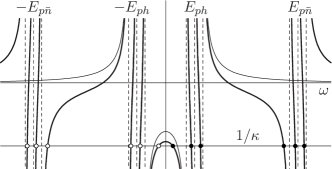
Figure 1: Graphical solution of the full RPA dispersion equation with Eq.(88). The thick and thin solid curves are calculated with and without the coupling with the N-$\mathrm{\overline{N}}$ states, respectively. The solid circles denote the eigenvalues of the RPA excited states. The vertical broken lines indicate the position of the unperturbed energies. For the details, see the text.

Fig.2 shows the dispersion relation with Eq.(89) of NSA and NFA. On the contrary to Fig.1, the lowest positive energy state is pushed up with the coupling, in spite of the fact that the interaction is assumed to be attractive. Moreover, except for low lying positive energy states around $E_{ph}$, the eigenvalues with $\lambda=1(dR/d\omega<0)$ appear at the negative energy region around $-E_{h\bar{n}}$ in both NSA and NFA.

In addition to the thick and thin curves as in Fig.1, the dotted curve is shown, which is obtained without the coupling and with a less number of particle-hole states. Compared with the thin curve, we see that the excitation energy of the lowest state is decreased with the increased number of the particle-hole states. Therefore, when the attractive force is enough for the spurious state with zero energy in NSA and NFA, its eigenvalue becomes imaginary in neglecting the coupling with N-$\mathrm{\overline{N}}$ states, because of $\kappa^{-1}=R^{\mathrm{ph}}(0)-R^{\mathrm{h\bar{n}}}(0)>R^{\mathrm{ph}}(0)$ as in Eq.(89). These dependence on the number of the configurations was also observed numerically in Ref.[10].

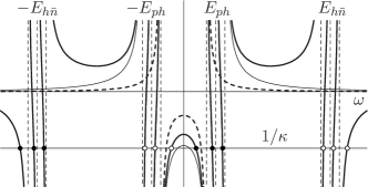
Figure 2: Same as Fig.1 for Eq.(89). The dotted curve is obtained without the N-$\mathrm{\overline{N}}$ coupling and with a less number of particle-hole states. For the details, see the text.

Finally, it may be useful to re-examine in the present RPA framework the relativistic Landau-Migdal parameters of the $\sigma$-$\omega$ model developed in Refs.[7, 17, 24]. In discussing the response of nuclear matter at low momentum transfer $q\approx 0$, the interaction Eq.(23) of the $\sigma$-$\omega$ model can be expressed as a separable form. It is written in Eq.(78) as

$$f^{(a)}_{\alpha\beta}=\frac{1}{\sqrt{\Omega}}\langle\,\overline{\alpha}\,|\,e^{i\boldsymbol{q}\cdot\boldsymbol{x}}\varGamma^{a}\,|\,\beta\,\rangle=\frac{\delta_{\boldsymbol{p}_{\alpha},\boldsymbol{p}_{\beta}+\boldsymbol{q}}}{\sqrt{\Omega}}\,\overline{w}_{\alpha}\varGamma^{a}w_{\beta}\,,\quad$$

with

$$\kappa_{a}=\left\{\begin{array}[]{ll}-\,f_{\sigma}=-\,g_{\sigma}^{2}/m_{\sigma}^{2}\,,&a=-\,1,\\[4.0pt] +\,f_{\omega}=g_{\omega}^{2}/m_{\omega}^{2}\,,&a=0,\\[4.0pt] -\,f_{\omega}\,,&a=1,\,2,\,3.\end{array}\right.$$

Here, $\Omega$ denotes the volume of the system which we need for rewriting the integral of Eqs.(9) and (10) with the summation, and $w_{\alpha}=w_{s}(\boldsymbol{p}\sigma)$ stands for the four-component spinor, $\alpha$ representing $\{s=\pm,\boldsymbol{p},\sigma\}$,

$$w_{+}(\boldsymbol{p}\sigma) =\sqrt{\frac{E_{\boldsymbol{p}}+M^{\ast}}{2E_{\boldsymbol{p}}}}\left(\begin{array}[]{c}1\\[4.0pt] \dfrac{\boldsymbol{\sigma}\!\cdot\!\boldsymbol{p}}{E_{\boldsymbol{p}}+M^{\ast}}\end{array}\right)\,\chi_{\sigma}\,,$$ (97)

$$w_{-}(\boldsymbol{p}\sigma) =\sqrt{\frac{E_{\boldsymbol{p}}+M^{\ast}}{2E_{\boldsymbol{p}}}}\left(\begin{array}[]{c}-\dfrac{\boldsymbol{\sigma}\!\cdot\!\boldsymbol{p}}{E_{\boldsymbol{p}}+M^{\ast}}\\[8.0pt] 1\end{array}\right)\,\chi_{\sigma}\,,$$ (100)

with $E_{\boldsymbol{p}}=\sqrt{\boldsymbol{p}^{2}+M^{\ast 2}}$ and the 2-component spinor, $\chi_{\sigma}$.

The matrix $R$ in Eq.(80) can be divided into the longitudinal and transverse part[6]. Taking $\boldsymbol{q}=(q,0,0)$, the former is the $3\times 3$ matrix depending on $a=-1,0$ and $1$, while the latter is composed of $a=2$ and $3$. The longitudinal part, which is required for the present discussions, is calculated in NFA and NSA as

$$D_{\mathrm{L}}=\mathrm{det}\Bigl{(}\delta_{ab}-\kappa_{a}R_{ab}(\omega)\Bigr{)}=\left|\begin{array}[]{ccc}C_{\sigma}+f_{\sigma}R^{\mathrm{ph}}_{\sigma}&f_{\sigma}R^{\mathrm{ph}}_{\sigma\omega}&sf_{\sigma}R^{\mathrm{ph}}_{\sigma\omega}\\[4.0pt] -\,f_{\omega}R^{\mathrm{ph}}_{\sigma\omega}&C^{0}_{\omega}-f_{\omega}R^{\mathrm{ph}}_{\omega}&-\,sf_{\omega}R^{\mathrm{ph}}_{\omega}\\[4.0pt] sf_{\omega}R^{\mathrm{ph}}_{\sigma\omega}&sf_{\omega}R^{\mathrm{ph}}_{\omega}&C^{1}_{\omega}+f_{\omega}s^{2}R^{\mathrm{ph}}_{\omega}\end{array}\right|$$ (101)

where we have used the following abbreviations,

$$C_{\sigma}=1-f_{\sigma}R^{\mathrm{h\bar{n}}}_{-1-1}\,,\qquad C^{0}_{\omega}=1+f_{\omega}R^{\mathrm{h\bar{n}}}_{00}\,,\qquad C^{1}_{\omega}=1-f_{\omega}\left(R^{\mathrm{h\bar{n}}}_{11}+\frac{N_{\mathrm{F}}v_{\mathrm{F}}^{2}}{3}\right),$$ (102)

together with $s=\omega/q$, $v_{\mathrm{F}}=p_{\mathrm{F}}/E_{p_{\mathrm{F}}}$ for the relativistic Fermi velocity and $N_{\mathrm{F}}=2v_{\mathrm{F}}E_{p_{\mathrm{F}}}^{2}/\pi^{2}$ for the relativistic density of states at the Fermi surface. Here $E_{p_{\mathrm{F}}}$ is defined by $\sqrt{p_{\mathrm{F}}^{2}+M^{\ast 2}}$, using the Fermi momentum $p_{\mathrm{F}}$. The function $R^{\mathrm{ph}}$ for isosymmetric nuclear matter is given by

$$R^{\mathrm{ph}}_{\sigma}=N_{\mathrm{F}}\left(1-v_{\mathrm{F}}^{2}\right)\varPhi(x)\\ ,\quad R^{\mathrm{ph}}_{\sigma\omega}=N_{\mathrm{F}}\sqrt{1-v_{\mathrm{F}}^{2}}\,\varPhi(x)\\ ,\quad R^{\mathrm{ph}}_{\omega}=N_{\mathrm{F}}\varPhi(x),$$

where $\varPhi(x)$ stands for Lindhard function with $x=\omega/v_{\mathrm{F}}q$,

$$\varPhi(x)=-\,1+\frac{x}{2}\log\left|\frac{1+x}{1-x}\right|-\frac{i\pi}{2}|x|\,\theta(\,1-|x|\,).$$ (103)

By writing the determinant Eq.(101) in terms of the Landau-Migdal parameters, $F_{0}$ and $F_{1}$, as [17]

$$\frac{D_{\mathrm{L}}}{C_{\sigma}C^{0}_{\omega}C^{1}_{\omega}} =1+\frac{f_{\sigma}}{C_{\sigma}}R^{\mathrm{ph}}_{\sigma}-\frac{f_{\omega}}{C^{0}_{\omega}}R^{\mathrm{ph}}_{\omega}+\frac{f_{\omega}}{C^{1}_{\omega}}s^{2}R^{\mathrm{ph}}_{\omega}$$

$$=1-\left(F_{0}+\frac{F_{1}}{1+F_{1}/3}x^{2}\right)\varPhi(x)\,,$$ (104)

we obtain

$$F_{0}=-\frac{(1-v_{\mathrm{F}}^{2})F_{\sigma}}{1-f_{\sigma}R^{\mathrm{h\bar{n}}}_{-1-1}}+\frac{F_{\omega}}{1+f_{\omega}R^{\mathrm{h\bar{n}}}_{00}}\ ,\quad F_{1}=-\frac{v_{\mathrm{F}}^{2}F_{\omega}}{1-f_{\omega}R^{\mathrm{h\bar{n}}}_{11}}\ ,\\$$ (105)

with $F_{\omega}=N_{\mathrm{F}}f_{\omega}$ and $F_{\sigma}=N_{\mathrm{F}}f_{\sigma}$. Thus, Pauli blocking terms yield the denominators depending on each meson exchange. They are calculated as,

$$R^{\mathrm{h\bar{n}}}_{-1-1}=-4\int_{0}^{p_{\mathrm{F}}}\!\!\frac{\mathrm{d}^{3}p}{(2\pi)^{3}}\frac{\boldsymbol{p}^{2}}{E^{3}_{\boldsymbol{p}}},\qquad R^{\mathrm{h\bar{n}}}_{00}=0\,,\qquad R^{\mathrm{h\bar{n}}}_{11}=-4\int_{0}^{p_{\mathrm{F}}}\!\!\frac{\mathrm{d}^{3}p}{(2\pi)^{3}}\frac{E^{2}_{\boldsymbol{p}}-\boldsymbol{p}^{2}/3}{E^{3}_{\boldsymbol{p}}},$$ (106)

It is seen that the attractive interactions are quenched by the Pauli blocking terms in the same way as in Eq.(93). In the present model, there is no contribution to the repulsive part, since $R^{\mathrm{h\bar{n}}}_{00}=0$ due to $f_{\alpha\neq\beta}^{(0)}=0$.

The parameter $F_{0}$ is responsible for the nuclear incompressibility coefficient, which determines the restoring force of giant monopole state. Reduction of the attractive part makes the value of the coefficient higher [7].

In contrast to $F_{0}$, the parameter $F_{1}$ is constrained by more fundamental requirement that the Femi energy $E_{\mathrm{F}}$ and momentum $p_{\mathrm{F}}$ are transformed as a four-vector [25]. In the $\sigma$-$\omega$ model, the parameter $F_{1}$ comes from the longitudinal part of the $\omega$-meson exchanges as a relativistic effect, while the nucleon effective mass stems from the $\sigma$-meson exchange. They, however, are not independent of each other, as in nonrelativistic models, and should satisfy, according to the above requirement[11],

$$\frac{E_{p_{\mathrm{F}}}}{E_{\mathrm{F}}}=1+\frac{F_{1}}{3}.$$ (107)

for $E_{\mathrm{F}}=E_{\mathrm{B}}+M$, $E_{\mathrm{B}}$ being the binding energy per nucleon. As far as Eq.(107) holds, $F_{1}$ describes correctly the center of mass motion by the Lorentz boost[8], and restores also an abnormal enhancement of magnetic moments due to the effective mass in the Hartree approximation[11]. Thus, although NFA and NSA seem to be consistent with the framework of the Landau-Migdal parameters, this fact does not imply that the divergence can be neglected.

We note that the last term $N_{\mathrm{F}}v_{\mathrm{F}}^{2}/3$ in $C^{1}_{\omega}$ of Eq.(102) comes from particle-hole excitations through the space component of the $\omega$-meson exchange

$$R^{\mathrm{ph}}_{11}=s^{2}R^{\mathrm{ph}}_{\omega}-\frac{N_{\mathrm{F}}v_{\mathrm{F}}^{2}}{3}.$$ (108)

Because of the last term, the continuity equation does not hold in the particle-hole space, $R^{\mathrm{ph}}_{11}\neq s^{2}R^{\mathrm{ph}}_{00}=s^{2}R^{\mathrm{ph}}_{\omega}$. NFA and NSA, however, take into account a part of N-$\mathrm{\overline{N}}$ states. The calculation of $R^{\mathrm{h\bar{n}}}_{11}$ in Eq.(106) provides $-N_{\mathrm{F}}v_{\mathrm{F}}^{2}/3$, which leads to the continuity equation, $R^{\mathrm{ph}}_{11}-R^{\mathrm{h\bar{n}}}_{11}=s^{2}(R^{\mathrm{ph}}_{00}-R^{\mathrm{h\bar{n}}}_{00})$, as discussed in §4.

7 Conclusions

The structure of the relativistic random phase approximation(RPA) has been investigated in detail. The energy-weighted sum of the RPA transition strengths is expressed formally as the Hartree ground-state expectation value of the double commutator between the excitation operator and the Hamiltonian, as in non-relativistic models. In calculating the commutator, however, the usual anticommutation relation between the baryon fields cannot be used[15]. Otherwise, the sum, which should be infinite[15], would vanish.

The main difference of the relativistic RPA from the nonrelativistic one stems from antinucleon($\mathrm{\overline{N}}$) degrees of freedom, but they cause the divergence problems. The two kinds of approximations were proposed by previous authors in order to avoid the problems without the renormalization. The one[5, 6] is the no free term approximation(NFA) which simply neglects the divergent terms in RPA response function, and the other[10] is the no-sea approximation(NSA) where $\mathrm{\overline{N}}$ states are assumed to be empty. Actually, both approximations are equivalent to each other. They were employed widely and shown to work well for reproducing experimental data in a phenomenological way[3, 6, 9, 10, 12, 13, 14].

The present paper has shown that NFA and NSA have the serious problems. The RPA dispersion equation yields the RPA states with negative excitation energy, in addition to the low lying positive energy states. This fact implies that the RPA ground state is not the lowest one. Owing to those negative excitation-energy states, the energy-weighted sum of the transition strengths vanishes. These results are not avoidable for NFA and NSA which satisfy the RPA relation of the energy-weighted strengths, since the relativistic sum rule value stems from the excitations of Dirac sea[15]. Moreover, since the only limited space of nucleon-antinucleon states is included in NFA and NSA, attractive(repulsive) forces work as repulsive(attractive) ones between their couplings. This fact affects also the couplings of the particle-hole states with nucleon-$\mathrm{\overline{N}}$ states. Unfortunately, these unphysical couplings played an important role in explaining the spurious state[10] and the giant monopole states[12, 13, 14] in the previous numerical calculations in NSA. These results have been shown clearly by using a schematic model.

It has been shown that there is no problem for NSA and NFA to describe the continuity equation, since it is independent of the divergence.

Thus, $\mathrm{\overline{N}}$ degrees of freedom which provide the divergence are not ignored. As far as a part of the $\mathrm{\overline{N}}$ space is necessary, the rest of the space also should be taken into account in a proper way, even in phenomenological models. Indeed, it was shown in Refs.[5, 7, 26, 27] that the renormalization of the divergence plays an important role in discussions of some physical quantities. Those roles are state-dependent, and could not be incorporated into phenomenological interactions or their coupling constants. Moreover, if the divergence of the linearly energy-weighted sum is understood, we can make clear the meaning of the analyses as to the distribution of transition strengths with the energy moments[4].

References

• [1] B. D. Serot and J. D. Walecka, Advance in Nuclear Physics, ed. E. Vogt and J. Negle (Plenum, New York, 1986), vol.16.
• [2] P. Ring, Prog. Part. Nucl. Phys., 37, 193 (1996).
• [3] H. Liang, T. Nakatsukasa, Z. Niu, and J. Meng, Phys. Rev. C, 87, 054310 (2013) and references therein.
• [4] W. C. Chen, J. Piekarewicz, and M. Centelles, Phys. Rev. C, 88, 024319 (2013).
• [5] S. A. Chin, Ann. Phys. (N. Y.), 108, 301 (1977).
• [6] H. Kurasawa and T. Suzuki, Nucl. Phys., A, 445, 685 (1985).
• [7] H. Kurasawa and T. Suzuki, Phys. Lett., B, 474, 262 (2000).
• [8] S. Nishizaki, H. Kurasawa, and T. Suzuki, Nucl. Phys. A, 462, 687 (1987).
• [9] J. R. Shepard, E. Rost, and J. A. McNeil, Phys. Rev. C, 40, 2320 (1989)
• [10] J. F. Dawson and R. J. Furnstahl, Phys. Rev. C, 42, 2009 (1990).
• [11] H. Kurasawa and T. Suzuki, Phys. Lett. B, 165, 234 (1985).
• [12] J. Piekarewicz, Phys. Rev. C, 64, 024307 (2001).
• [13] Z. Ma, N. Van Giai, A. Wandelt, D. Vretnar, and P. Ring, Nucl. Phys. A, 686, 173 (2001);
• [14] Z. Ma, L. Cao, N. Van Giai, and P. Ring, Nucl. Phys. A, 722, C491(2003).
• [15] H. Kurasawa and T. Suzuki, Prog. Theor. Exp. Phys., 2013, 043D04 (2013).
• [16] D. J. Rowe, Nuclear Collective Motion, Models and Theory (World Scientific Publishing, Singapore, 2010).
• [17] H. Kurasawa and T. Suzuki, Nucl. Phys. A, 454, 527 (1986).
• [18] A. L. Fetter and J. D. Walecka, Quantum Theory of Many-Particle Systems, (MacGrow-Hill Book Company, New York, 1971).
• [19] D. J. Thouless, Nucl. Phys., 22, 78 (1961).
• [20] T. Goto and T. Inamura, Prog. Theor. Phys., 14, 396 (1955).
• [21] J. Schwinger, Phy. Rev. Lett., 3, 296 (1959).
• [22] C. Itzykson and J. B. Zuber, Quantum Field Theory (McGraw Hill, New York, 1986), p.530.
• [23] H. Kurasawa and T. Suzuki, Phys. Rev. C, 69, 014306 (2004).
• [24] T. Matsui, Nucl. Phys. A, 370, 365 (1981).
• [25] G. Baym and S. A. Chin, Nucl. Phys. A, 262, 527 (1976).
• [26] H. Kurasawa and T. Suzuki, Nucl. Phys. A, 490, 571 (1988).
• [27] H. Kurasawa and T. Suzuki, Mod. Phys. Lett. A, 21, 935 (2006).