Resonant-state-expansion Born approximation for waveguides with dispersion

Abstract

The resonant-state expansion (RSE) Born approximation, a rigorous perturbative method developed for electrodynamic and quantum mechanical open systems, is further developed to treat waveguides with a Sellmeier dispersion. For media that can be described by these types of dispersion over the relevant frequency range, such as optical glass, I show that the perturbed RSE problem can be solved by diagonalizing a second-order eigenvalue problem. In the case of a single resonance at zero frequency, this is simplified to a generalized eigenvalue problem. Results are presented using analytically solvable planar waveguides and parameters of borosilicate BK7 glass, for a perturbation in the waveguide width. The efficiency of using either an exact dispersion over all frequencies or an approximate dispersion over a narrow frequency range is compared. I included a derivation of the RSE Born approximation for waveguides to make use of the resonances calculated by the RSE, an RSE extension of the well-known Born approximation.

I Introduction

Fundamental to scattering theory, the Born approximation consists of taking the incident field in place of the total field as the driving field at each point inside the scattering potential, it was first discovered by Born and presented in Ref. Born26 . The Born approximation gave an expression for the differential scattering cross section in terms of the Fourier transform of the scattering potential. An important feature of this appearance of the Fourier transform is the availability of the inverse Fourier transform operation for the inverse scattering problem. The Born approximation is only valid for weak scatterers. In this paper I apply the RSE Born approximation Ref.DoostARX15 ; Ge14 to optical fibers or general open waveguide systems, which allows an arbitrary number of resonant-states (RSs) to be taken into account for scattering and transmission perturbative calculations.

Optical fibers provide a well-controlled optical path which can carry light over potentially very long distances of several hundred to thousands of kilometers since the light is contained within the fiber by total internal reflection. Fibers are clearly important for telecommunication since the light may be modulated to carry information. It has recently been reported that a hollow-core photonic-band gap fiber yielded a record combination of low loss and wide bandwidth Poletti13 . Beyond telecommunications waveguides are used in integrated optical circuits John09 , and terabit chip-to-chip interconnects Gonzalez12 .

Critical to understanding the response of a waveguide to being optically driven are its resonant states (RSs). The concept of RSs was first conceived and used by Gamow in 1928 in order to describe mathematically the process of radioactive decay, specifically the escape from the nuclear potential of an $\alpha$ particle by tunneling. Mathematically this corresponded to solving Schrödinger’s equation for outgoing boundary conditions (BCs). These states have complex frequency $\omega$ with negative imaginary part meaning their time dependence $\exp(-i\omega t)$ decays exponentially, thus giving an explanation for the exponential decay law of nuclear physics. The consequence of this exponential decay with time is that the further from the decaying system at a given instant of time, the greater the wave amplitude. An intuitive way of understanding this divergence of wave amplitude with distance is to notice that waves that are further away have left the system at an earlier time when less of the particle probability density had leaked out. There already exists numerical techniques for finding eigenmodes, such as the finite element method (FEM) and finite difference in time domain (FDTD) method to calculate resonances in open cavities. However, determining the effect of perturbations, which break the symmetry, presents a significant challenge as these popular computational techniques need large computational resources to model high-quality modes. Also these methods generate spurious solutions, which would damage the accuracy of the RSE Born approximation if included in the perturbation expansion basis.

In order to calculate the resonances of open systems we have recently developed the resonant-state expansion. Such an approach was not previously available due to the lack of a normalization for resonant states. I derived the normalization of resonant states as a contribution to Ref.DoostPRA14 , and the generalization of the normalisation to dispersive media I derived straight forwardly at the time of my rigorous derivation. The problem of normalising resonant states stems from the fact that RSs with complex frequencies have wave functions which are exponentially growing in space away from system, making a volume integral over all space as would be done for a hermitian system a meaningless exercise (see Appendix F). However the ${\it S}$-wave normalization was previously available and analytically correct but numerically unstable as I showed analytically in Ref DoostARX15 .

So far the RSE has been applied to non dispersive systems of different dimensionality MuljarovEPL10 ; DoostPRA12 ; DoostPRA13 ; ArmitagePRA14 ; DoostPRA14 . However, almost all realistic systems have a relevant frequency dispersion of the refractive index. I have recently found Doost15 ; DoostARX15 that an Ohm’s law dispersion, i.e. a term in the susceptibility scaling at the inverse frequency, can be introduced to the RSE while keeping its linearity. We found in Ref.Doost15 this dispersion can be a reasonable approximation for some materials over a limited range of wavelengths such as SHOTT BK7 glass over the optical range. In this work I generalize the RSE approach for waveguides detailed in Ref.ArmitagePRA14 to systems constructed from dispersive media. Specifically I treat dispersion fully described by the Sellmeier equation, using a method similar to Muljarov et al in Ref.Egor for nano particles obeying Drude-Lorentz dispersion, however in this case generalised to inclined geometry. I also treat dispersion linear in wavelength squared, a generalisation of my work in Ref.Doost15 ; DoostARX15 to inclined geometry. I find the generalization of my Ohm’s law approach to inclined geometry to be greatly superior to the generalization of the full dispersion treatment. This is most likely due to the unphysicality of the full dispersion at high and low frequencies, which are beyond the fitting range of the dispersion models. In order to make use of the RSs, I derive the RSE Born approximation for waveguides DoostARX15 ; Ge14 , a theory for finding the field outside of a waveguide being internally or externally driven (see Appendix G).

The paper is organized as follows, Sec. II outlines the general recursive solution of Maxwell’s equation using Green’s function. Sec. III develops the solution in Sec. II into a perturbation theory for waveguides with linear dispersion in wavelength squared. Sec. IV develops the solution in Sec. II into a perturbation theory for waveguides with Sellmeier dispersion. Sec. VI demonstrates and compares the two approaches for including dispersion into the RSE. The perturbation considered corresponds to a narrowing of the waveguide and is discussed in Sec. VI.3. In Sec. VI.4 I show the results using the simple dispersive approximation BK7. In Sec. VI.5 I use the full Sellmeier dispersion of BK7. Finally, we discuss the comparison and performance of the two methods in Sec. VI.6, in Sec. VII, I derive the equations for the RSE Born approximation for planar waveguides. In Appendix C, D, E, and F I generalize my part of the proof of the normalization of RSs to open waveguide systems.

II Resonant state expansion for waveguides and non-normal incidence

In this section I develop the general recursive solution to the problem of calculating the resonant states of a perturbed waveguide. The recursive solution requires the Green’s function (GF) of the unperturbed waveguide, and a perturbation which is retaining the translational invariance along the waveguide.

I first consider a waveguide of thickness $2a$ in vacuum with translational invariance in one direction, having the dielectric constant

$$\hat{\boldsymbol{\varepsilon}}_{\omega}(\mathbf{\dot{r}})=\left\{\begin{array}[]{cl}\epsilon_{\rm\omega}&\text{for\ \ }|\mathbf{\dot{r}}|\leqslant a\,,\\ 1&\text{for\ \ }|\mathbf{\dot{r}}|>a\,,\end{array}\right.$$ (1)

where $\epsilon_{\rm\omega}$ is the frequency dependent relative permittivity (RP) of the wave guide with the angular frequency $\omega$. $\mathbf{\dot{r}}$ are the coordinates normal to the waveguide, which for a cylindrical waveguide is given in polar coordinates $\mathbf{\dot{r}}=(\rho,\theta)$ and for a planar waveguide $\mathbf{\dot{r}}$ is Cartesian $x$. I assume a relative permeability of $\mu=1$ throughout this work. The electric field ${\bf\hat{E}}$ satisfies Maxwell’s equation,

$$\left[-\nabla\times\nabla\times-\hat{\boldsymbol{\varepsilon}}_{\omega}(\mathbf{r})\frac{1}{c^{2}}\frac{\partial^{2}}{\partial t^{2}}\right]{\bf\hat{E}}({\bf r},t)=0\,,$$ (2)

For cylindrical and planar waveguides, due to translational invariance in the $z$ direction I first assume then prove that ${\bf\hat{E}}$ can be factorised as follows

$${\bf\hat{E}}({\bf r},t)=e^{i(pz-\omega t)}{\bf E}(\mathbf{\dot{r}})\,,$$ (3)

in which $p$ is the wave vector along the translationally invariant direction. For the component ${\bf E}(\mathbf{\dot{r}})$ of the electric field, Eq. (2) transforms to a one-dimensional (1D) wave equation in the planar case or a 2D wave-equation for the cylindrical waveguide to

$$\left[-L+\hat{\boldsymbol{\varepsilon}}_{\omega}(\mathbf{\dot{r}})\frac{\omega^{2}}{c^{2}}\right]{\bf E}(\mathbf{\dot{r}})=0\,.$$ (4)

Here $L$ is a linear operator not dependent on $z$ or $\hat{\boldsymbol{\varepsilon}}_{\omega}(\mathbf{\dot{r}})$. The form of $L$ is derived in Appendix C, the derivation shows that the trial solution Eq. (3) is correct since it demonstrates that ${\bf\hat{E}}$ can be factorised by separation of variables. In principle $L$ could be any linear operator independent of both $z$ and $\hat{\boldsymbol{\varepsilon}}_{\omega}(\mathbf{\dot{r}})$, and hence the treatment of waveguides in this paper is readily applicable to quantum mechanics or acoustics.

The non-normal incidence, characterized by $p\neq 0$, is treated here. The previously used spectral representation of the GF in the frequency domain contains a cut for $p\neq 0$, which can be removed by mapping the problem onto the complex normal wave-vector space $k$, as demonstrated in Ref.ArmitagePRA14 . The relation between $k$, $p$, and $\omega$ is defined by us to be $\omega^{2}/c^{2}=k^{2}+p^{2}$, $k$ and $p$ are orthogonal by Pythagorean identity. I follow also here the approach used in Ref.ArmitagePRA14 and formulate the RSE in the complex $k$-plane, for which the spectral representation of the GF of an infinite planar system with an in-plane momentum $p\neq 0$ written in the spectral form

$${\hat{\mathbf{G}}^{(1)}_{k}}(\mathbf{\dot{r}},\mathbf{\dot{r}}^{\prime})=\sum_{n}\frac{{\bf E_{n}}(\mathbf{\dot{r}})\otimes{\bf E_{n}}(\mathbf{\dot{r}}^{\prime})}{2k_{n}(k-k_{n})}\,,$$ (5)

where ${\bf E_{n}}(\mathbf{\dot{r}})$ is the electric field of a RS, defined as an eigensolution of Eq. (4) with an arbitrary profile of $\hat{\boldsymbol{\varepsilon}}_{\omega}(\mathbf{\dot{r}})$ within a region $|\mathbf{\dot{r}}|<a$, satisfying the outgoing wave boundary conditions at infinity. The dyadic product of the ${\bf E_{n}}(\mathbf{\dot{r}})$ fields is denoted by $\otimes$. The in-plane eigenfrequency $k_{n}$ are the poles in ${\hat{\mathbf{G}}_{k}}(\mathbf{\dot{r}},\mathbf{\dot{r}}^{\prime})$. By definition $\omega^{2}_{n}/c^{2}=k_{n}^{2}+p^{2}$ where $\omega^{2}_{n}$ is the eigenfrequency corresponding to the eigenstate ${\bf E_{n}}(\mathbf{\dot{r}})$. For a study of the derivation of such spectral representations see Appendix D.

The GF satisfies the equation

$$\left[-L+\hat{\boldsymbol{\varepsilon}}_{\omega}(\mathbf{\dot{r}})(k^{2}+p^{2})\right]{\hat{\mathbf{G}}_{k}}(\mathbf{\dot{r}},\mathbf{\dot{r}}^{\prime})=\hat{\mathbf{1}}\delta(\mathbf{\dot{r}}-\mathbf{\dot{r}}^{\prime})$$ (6)

In the present work, we consider the refractive profile (RP) having the property

$$\lim_{\omega\rightarrow\infty}\hat{\boldsymbol{\varepsilon}}_{\omega}(\mathbf{\dot{r}})=\hat{\boldsymbol{\varepsilon}}(\mathbf{\dot{r}}),$$ (7)

where $\hat{\boldsymbol{\varepsilon}}(\mathbf{\dot{r}})$ if the frequency independent part of $\hat{\boldsymbol{\varepsilon}}_{\omega}(\mathbf{\dot{r}})$. If we assume $\hat{\boldsymbol{\varepsilon}}_{\omega}(\mathbf{\dot{r}})$ to be discontinuous through the boundary of the system then by substituting Eq. (5) into Eq. (6), convoluting with a finite function, and letting $k\rightarrow\infty$, we obtain the sum rule (see Appendix E)

$$\sum_{n}\frac{{\bf E_{n}}(\mathbf{\dot{r}})\otimes{\bf E_{n}}(\mathbf{\dot{r}}^{\prime})}{k_{n}}=0\,,$$ (8)

which allows us to re-write the Green’s function a second way as

$${\hat{\mathbf{G}}^{(2)}_{k}}(\mathbf{\dot{r}},\mathbf{\dot{r}}^{\prime})=\sum_{n}\frac{{\bf E_{n}}(\mathbf{\dot{r}})\otimes{\bf E_{n}}(\mathbf{\dot{r}}^{\prime})}{2k_{n}}\left[\frac{1}{k-k_{n}}-\dfrac{k}{k^{2}+p^{2}}\right]\,,$$ (9)

I now consider an arbitrary perturbation $\Delta\hat{\boldsymbol{\varepsilon}}_{\omega}(\mathbf{\dot{r}})$ of the dielectric constant inside the layer $|\mathbf{\dot{r}}|<a$. I use the Eq. (6) to solve the perturbed problem,

$$\mbox{\boldmath${\cal E}$}_{\nu}(\mathbf{\dot{r}})=-\frac{\omega^{2}}{c^{2}}\int\hat{\mathbf{G}}_{k}(\mathbf{\dot{r}},\mathbf{\dot{r}}^{\prime})\Delta\hat{\boldsymbol{\varepsilon}}_{\omega}(\mathbf{\dot{r}}^{\prime})\mbox{\boldmath${\cal E}$}_{\nu}(\mathbf{\dot{r}}^{\prime})d{\bf\mathbf{\dot{r}}}^{\prime}\,,$$ (10)

which is the solution to the equation

$$L\mbox{\boldmath${\cal E}$}_{\nu}(\mathbf{\dot{r}})=\frac{\omega^{2}}{c^{2}}\left[\hat{\boldsymbol{\varepsilon}}_{\omega}(\mathbf{\dot{r}})+\Delta\hat{\boldsymbol{\varepsilon}}_{\omega}(\mathbf{\dot{r}})\right]\mbox{\boldmath${\cal E}$}_{\nu}(\mathbf{\dot{r}})$$ (11)

Note that the perturbed modes $\mbox{\boldmath${\cal E}$}_{\nu}(\mathbf{\dot{r}})$ satisfy Eq. (4) with $\hat{\boldsymbol{\varepsilon}}_{\omega}(\mathbf{\dot{r}})$ replaced by $\hat{\boldsymbol{\varepsilon}}_{\omega}(\mathbf{\dot{r}})+\Delta\hat{\boldsymbol{\varepsilon}}_{\omega}(\mathbf{\dot{r}})$ and the outgoing boundary conditions with $\omega_{n}$ replaced by $\omega$. I show the solution of this equation perturbatively for two different types of dispersion in the following two sections.

III Single Sellmeier resonance at zero frequency

For a Sellmeier dispersion with a single resonance at zero frequency (SRZ), I write the perturbation in Eq. (10) as

$$\Delta\hat{\boldsymbol{\varepsilon}}_{\omega}(\mathbf{\dot{r}})=\Delta\hat{\boldsymbol{\varepsilon}}(\mathbf{\dot{r}})+\frac{c^{2}\Delta\hat{\boldsymbol{\sigma}}(\mathbf{\dot{r}})}{\omega^{2}}\,,$$ (12)

again present only inside the layer $|\mathbf{\dot{r}}|<a$. It is then possible to linearise the RSE by using the different forms of the Green’s function, similar to Ref.Egor , Eq. (5) and Eq. (9) for the different components of the perturbation in Eq. (10),

$$\mbox{\boldmath${\cal E}$}(\mathbf{\dot{r}}) = -\int\hat{\mathbf{G}}^{(1)}_{k}(\mathbf{\dot{r}},\mathbf{\dot{r}}^{\prime})\Delta\hat{\boldsymbol{\sigma}}(\mathbf{\dot{r}}^{\prime})\mbox{\boldmath${\cal E}$}(\mathbf{\dot{r}}^{\prime})d{\bf\mathbf{\dot{r}}}^{\prime}$$ (13)

$$-\frac{\omega^{2}}{c^{2}}\int\hat{\mathbf{G}}^{(2)}_{k}(\mathbf{\dot{r}},\mathbf{\dot{r}}^{\prime})\Delta\hat{\boldsymbol{\varepsilon}}(\mathbf{\dot{r}}^{\prime})\mbox{\boldmath${\cal E}$}(\mathbf{\dot{r}}^{\prime})d{\bf\mathbf{\dot{r}}}^{\prime}\,,$$

which results in the following relationship between unperturbed and perturbed modes

$$\mbox{\boldmath${\cal E}$}(\mathbf{\dot{r}}) = -\left(k^{2}+p^{2}\right)\sum_{n}\frac{{\bf E_{n}}(\mathbf{\dot{r}})}{2k_{n}}\left[\frac{1}{k-k_{n}}-\dfrac{k}{k^{2}+p^{2}}\right]$$ (14)

$$\times\int^{a}_{-a}{\bf E_{n}}(\mathbf{\dot{r}}^{\prime})\Delta\hat{\boldsymbol{\varepsilon}}(\mathbf{\dot{r}}^{\prime})\mbox{\boldmath${\cal E}$}(\mathbf{\dot{r}}^{\prime})d\mathbf{\dot{r}}$$

$$-\sum_{n}\frac{{\bf E_{n}}(\mathbf{\dot{r}})}{2k_{n}(k-k_{n})}$$

$$\times\int^{a}_{-a}{\bf E_{n}}(\mathbf{\dot{r}}^{\prime})\Delta\hat{\boldsymbol{\sigma}}(\mathbf{\dot{r}}^{\prime})\mbox{\boldmath${\cal E}$}(\mathbf{\dot{r}}^{\prime})d\mathbf{\dot{r}}\,.$$

The perturbed mode $\mbox{\boldmath${\cal E}$}(\mathbf{\dot{r}})$ satisfies Eq. (4) with $\hat{\boldsymbol{\varepsilon}}_{\omega}(\mathbf{\dot{r}})$ replaced by $\hat{\boldsymbol{\varepsilon}}_{\omega}(\mathbf{\dot{r}})+\Delta\hat{\boldsymbol{\varepsilon}}_{\omega}(\mathbf{\dot{r}})$ and outgoing boundary conditions with the wave vector $k$. In the interior region $\left|\mathbf{\dot{r}}\right|<a$ which contains the perturbation, the perturbed RSs $\mbox{\boldmath${\cal E}$}_{\nu}$ of wavenumbers $\varkappa_{\nu}$ can be expanded into the unperturbed ones, exploiting the completeness of the latter which follows from Eq. (72) (see also Appendix E),

$$\mbox{\boldmath${\cal E}$}_{\nu}(\mathbf{\dot{r}})=\sum_{n}b_{n\nu}{\bf E_{n}}(\mathbf{\dot{r}})\,.$$ (15)

Substituting this expansion into Eq. (13) and equating coefficients at the same basis functions ${\bf E_{n}}$ results in the matrix equation

$$b_{n\nu}=\sum_{m}-b_{m\nu}\frac{(p^{2}+\varkappa_{\nu}k_{n})V_{nm}+S_{nm}}{2k_{n}(\varkappa_{\nu}-k_{n})}\,,$$ (16)

where

$$V_{nm}=\int{{\bf E_{n}}(\mathbf{\dot{r}})\cdot\Delta\hat{\boldsymbol{\varepsilon}}(\mathbf{\dot{r}}){\bf E_{m}}(\mathbf{\dot{r}})\,d\mathbf{\dot{r}}}$$ (17)

and

$$S_{nm}=\int{{\bf E_{n}}(\mathbf{\dot{r}})\cdot\Delta\hat{\boldsymbol{\sigma}}(\mathbf{\dot{r}}){\bf E_{m}}(\mathbf{\dot{r}})\,d\mathbf{\dot{r}}}.$$ (18)

With the substitution $c_{n\nu}=b_{n\nu}\sqrt{k_{n}}$, Eq. (16) can be rewritten as

$$0=\sum_{m}c_{m\nu}\left\{\varkappa_{\nu}\left(\!\frac{\delta_{nm}}{k_{n}}\!+\!\frac{V_{nm}}{2\sqrt{k_{n}}\sqrt{k_{m}}}\!\right)\right.\\ \left.+\frac{p^{2}V_{nm}+S_{nm}}{2k_{n}\sqrt{k_{n}}\sqrt{k_{m}}}-\delta_{nm}\right\}$$ (19)

care should be taken to take the sign of $\sqrt{k_{a}}$ consistently between matrix elements. Eq. (19) is linear in $\varkappa_{\nu}$ and can be solved by libraries for generalized linear matrix eigenvalue problems. In the absence of dispersion, $S_{nm}=0$, and Eq. (19) reverts back to the expression for non-dispersive waveguides ArmitagePRA14 . In the absence of $p$, $pa=0$, we see that Eq. (19) reverts to an expression for dispersive perturbation to nano-particles Doost15 .

IV Sellmeier dispersion

In this section I develop the existing RSE for wave guides into a perturbation theory for waveguides with Sellmeier dispersion, following a similar approach to Ref.Egor . The Sellmeier dispersion is the sum of a set of Lorentzians in frequency with poles $q_{j}$ on the real axis. The starting point for this derivation is Eq. (10), the recursive solution for the perturbed problem derived in Sec. II.

In this section, we consider the RP

$$\hat{\boldsymbol{\varepsilon}}_{\omega}(\mathbf{\dot{r}})+\sum_{j}\dfrac{c^{2}\hat{\boldsymbol{\sigma}}_{j}(\mathbf{\dot{r}})}{\omega^{2}-\Omega^{2}_{j}},$$ (20)

and perturbation,

$$\Delta\hat{\boldsymbol{\varepsilon}}_{\omega}(\mathbf{\dot{r}})=\Delta\hat{\boldsymbol{\varepsilon}}(\mathbf{\dot{r}})+\sum_{j}\dfrac{c^{2}\Delta\hat{\boldsymbol{\sigma}}_{j}(\mathbf{\dot{r}})}{\omega^{2}-\Omega^{2}_{j}},$$ (21)

with $j$ numbering the resonances at frequencies $\Omega_{j}$ having oscillator strengths $\hat{\boldsymbol{\sigma}}_{j}$. We introduce an effective resonance wave vector $\hat{q}_{j}$ as $\hat{q}^{2}_{j}=\Omega_{j}^{2}/c^{2}-p^{2}$ and re-write Eq. (21) as,

$$\Delta\hat{\boldsymbol{\varepsilon}}_{\omega}(\mathbf{\dot{r}}) = \Delta\hat{\boldsymbol{\varepsilon}}(\mathbf{\dot{r}})+\sum_{j}\dfrac{\Delta\hat{\boldsymbol{\sigma}}_{j}(\mathbf{\dot{r}})}{k^{2}-\hat{q}^{2}_{j}}$$

$$= \Delta\hat{\boldsymbol{\varepsilon}}(\mathbf{\dot{r}})+\sum_{j}\left(\dfrac{\Delta\hat{\boldsymbol{\sigma}}_{j}(\mathbf{\dot{r}})}{2k(k-\hat{q}_{j})}+\dfrac{\Delta\hat{\boldsymbol{\sigma}}_{j}(\mathbf{\dot{r}})}{2k(k+\hat{q}_{j})}\right),$$

In the Appendix A I use my method of DoostARX15 , which was first adapted for full dispersion of 3D nano-particles by E. A. Muljarov in Ref.Egor , to derive for non-vanishing $\hat{\boldsymbol{\sigma}}_{j}$ the sum rule

$$\sum_{n}\frac{{\bf E_{n}}(\mathbf{\dot{r}})\otimes{\bf E_{n}}(\mathbf{\dot{r}}^{\prime})}{2k_{n}(k_{n}\pm\hat{q}_{j})}=0\,.$$ (23)

which allows us to write the Green’s function as

$${\hat{\mathbf{G}}^{(\pm j)}_{k}}(\mathbf{\dot{r}},\mathbf{\dot{r}}^{\prime})=\sum_{n}\frac{{\bf E_{n}}(\mathbf{\dot{r}})\otimes{\bf E_{n}}(\mathbf{\dot{r}}^{\prime})(k\pm\hat{q}_{j})}{2k_{n}(k-k_{n})(k_{n}\pm\hat{q}_{j})}\,,$$ (24)

which has the useful $(k\pm\hat{q}_{j})$ in the numerator for reducing the order of the perturbation matrix problem through cancellation with perturbation denominators which would otherwise have lead to high order polynomial eigen problems.

We now consider a perturbation $\Delta\hat{\boldsymbol{\varepsilon}}_{\omega}(\mathbf{\dot{r}})$ of the RP inside the layer $|\mathbf{\dot{r}}|<a$. Similar to the previous section we use the Eq. (6) to solve the perturbed problem,

$$\mbox{\boldmath${\cal E}$}(\mathbf{\dot{r}})=-\frac{\omega^{2}}{c^{2}}\int\hat{\mathbf{G}}_{k}(\mathbf{\dot{r}},\mathbf{\dot{r}}^{\prime})\Delta\hat{\boldsymbol{\varepsilon}}_{\omega}(\mathbf{\dot{r}}^{\prime})\mbox{\boldmath${\cal E}$}(\mathbf{\dot{r}}^{\prime})d{\bf\mathbf{\dot{r}}}^{\prime}\,,$$ (25)

where we take $\Delta\hat{\boldsymbol{\varepsilon}}_{\omega}(\mathbf{\dot{r}})$ of the same form as Eq. (IV). Using both forms of the Green’s function Egor , Eq. (9) and Eq. (24) in Eq. (25), yields

$$\mbox{\boldmath${\cal E}$}(\mathbf{\dot{r}}) = -\frac{\omega^{2}}{c^{2}}\int\hat{\mathbf{G}}^{(2)}_{k}(\mathbf{\dot{r}},\mathbf{\dot{r}}^{\prime})\Delta\hat{\boldsymbol{\varepsilon}}(\mathbf{\dot{r}}^{\prime})\mbox{\boldmath${\cal E}$}(\mathbf{\dot{r}}^{\prime})d{\bf\mathbf{\dot{r}}}^{\prime}$$

$$-\frac{\omega^{2}}{c^{2}}\sum_{\pm,j}\int G^{(\pm j)}_{k}(\mathbf{\dot{r}},\mathbf{\dot{r}}^{\prime})\dfrac{\Delta\hat{\boldsymbol{\sigma}}_{j}(\mathbf{\dot{r}}^{\prime})}{2k(k\pm\hat{q}_{j})}\mbox{\boldmath${\cal E}$}(\mathbf{\dot{r}}^{\prime})d{\bf\mathbf{\dot{r}}}^{\prime}\,,$$

which results in the following relationship between unperturbed and perturbed modes

$$\mbox{\boldmath${\cal E}$}(\mathbf{\dot{r}}) = -\left(k^{2}+p^{2}\right)\sum_{n}\frac{{\bf E_{n}}(\mathbf{\dot{r}})}{2k_{n}}\left[\frac{1}{k-k_{n}}-\dfrac{k}{k^{2}+p^{2}}\right]$$ (27)

$$\times\int{\bf E_{n}}(\mathbf{\dot{r}}^{\prime})\Delta\hat{\boldsymbol{\varepsilon}}(\mathbf{\dot{r}}^{\prime})\mbox{\boldmath${\cal E}$}(\mathbf{\dot{r}}^{\prime})d\mathbf{\dot{r}}^{\prime}$$

$$-\left(k^{2}+p^{2}\right)\sum_{n,\pm,j}\frac{{\bf E_{n}}(\mathbf{\dot{r}})(k\pm\hat{q}_{j})}{2k_{n}(k_{n}\pm\hat{q}_{j})(k-k_{n})}$$

$$\times\int{\bf E_{n}}(\mathbf{\dot{r}}^{\prime})\dfrac{\Delta\hat{\boldsymbol{\sigma}}_{j}(\mathbf{\dot{r}}^{\prime})}{2k(k\pm\hat{q}_{j})}\mbox{\boldmath${\cal E}$}(\mathbf{\dot{r}}^{\prime})d\mathbf{\dot{r}}^{\prime}\,.$$

The perturbed mode $\mbox{\boldmath${\cal E}$}(\mathbf{\dot{r}})$ satisfies Eq. (4) with $\hat{\boldsymbol{\varepsilon}}_{\omega}(\mathbf{\dot{r}})$ replaced by $\hat{\boldsymbol{\varepsilon}}_{\omega}(\mathbf{\dot{r}})+\Delta\hat{\boldsymbol{\varepsilon}}_{\omega}(\mathbf{\dot{r}})$ and outgoing boundary conditions with the wave vector $k$. In the interior region $\left|\mathbf{\dot{r}}\right|<a$ which contains the perturbation, the perturbed RSs $\mbox{\boldmath${\cal E}$}_{\nu}$ of wavenumbers $\varkappa_{\nu}$ can be expanded into the unperturbed ones, exploiting the completeness of the latter which follows from Eq. (72) (see also Appendix E),

$$\mbox{\boldmath${\cal E}$}_{\nu}(\mathbf{\dot{r}})=\sum_{n}b_{n\nu}{\bf E_{n}}(\mathbf{\dot{r}})\,.$$ (28)

Substituting this expansion into Eq. (27) and equating coefficients at the same basis functions ${\bf E_{n}}$ results in the matrix equation

$$b_{n\nu} = -\frac{p^{2}+\varkappa_{\nu}k_{n}}{2k_{n}(\varkappa_{\nu}-k_{n})}\sum_{m}V_{nm}b_{m\nu}$$ (29)

$$-\dfrac{(\varkappa_{\nu}^{2}+p^{2})}{2\varkappa_{\nu}(\varkappa_{\nu}-k_{n})}\sum_{m,j}\dfrac{A^{(j)}_{nm}}{k_{n}^{2}-\hat{q}^{2}_{j}}b_{m\nu}\,,$$

where

$$V_{nm}=\int{{\bf E_{n}}(\mathbf{\dot{r}})\cdot\Delta\hat{\boldsymbol{\varepsilon}}(\mathbf{\dot{r}}){\bf E_{m}}(\mathbf{\dot{r}})\,d\mathbf{\dot{r}}}$$ (30)

and

$$A^{(j)}_{nm}=\int{{\bf E_{n}}(\mathbf{\dot{r}})\cdot\Delta\hat{\boldsymbol{\sigma}}_{j}(\mathbf{\dot{r}}){\bf E_{m}}(\mathbf{\dot{r}})\,d\mathbf{\dot{r}}}$$ (31)

is the matrix of the perturbation in the basis of unperturbed RSs. Introducing the abbreviation

$$U_{nm}=\sum_{j}\dfrac{A^{(j)}_{nm}}{2(k^{2}_{n}-\hat{q}^{2}_{j})}$$ (32)

I arrive at

$$\sum_{m}b_{m\nu}\left\{p^{2}U_{nm}+\varkappa_{\nu}\left(\dfrac{p^{2}V_{nm}}{2k_{n}}-\delta_{nm}k_{m}\right)\right.\\ \left.+\varkappa_{\nu}^{2}\left(\delta_{nm}+\dfrac{V_{nm}}{2}+U_{nm}\right)\right\}=0\,,$$ (33)

which is of second order in $\varkappa_{\nu}$. We can write this matrix problem compactly as $\mathbf{Q}(\varkappa_{\nu})\mathbf{b}_{\nu}=0$ with $\mathbf{Q}(\varkappa_{\nu})=\varkappa_{\nu}^{2}\mathbf{M}+\varkappa_{\nu}\mathbf{C}+\mathbf{K}$. To solve this matrix problem for a basis of size $N$, I follow Ref.TisseurBOOK2001 and use the first companion linearization, defining

$$\mathbf{R}(\varkappa_{\nu})=\varkappa_{\nu}\begin{bmatrix}\mathbf{M}&0\\ 0&\mathbf{I}\end{bmatrix}+\begin{bmatrix}\mathbf{C}&\mathbf{K}\\ -\mathbf{I}&0\end{bmatrix}$$ (34)

where $\mathbf{I}$ is the $N$-by-$N$ identity matrix. with the corresponding vector

$$\mathbf{z}=\begin{bmatrix}\varkappa_{\nu}\mathbf{b}_{\nu}\\ \mathbf{b}_{\nu}\end{bmatrix}$$ (35)

We solve $\mathbf{R}(\varkappa_{\nu})\mathbf{z}=0$ using the generalized eigenvalue solver from the numerical algorithms group (NAG) C++ library. We then take the first $N$ components of $\mathbf{z}$ as the eigenvector $\mathbf{b}_{\nu}$.

V Possible explanation for the difference in order between the two methods

Here I go beyond the algebraic mathematics presented so far and discuss the fundamental topological differences between the two RSE approaches that I have developed.

The RSE perturbation theory presented here is an injective continuous mapping function except in the neighbourhood of the finite number of poles such that,

$$\hat{\boldsymbol{\varepsilon}}_{\omega}\omega^{2}=[\hat{\boldsymbol{\varepsilon}}_{\omega}\omega^{2}]^{(\rm reg)}+\sum_{j}[\hat{\boldsymbol{\varepsilon}}^{j}_{\omega}\omega^{2}]^{(\rm poles)}$$ (36)

is mapped to

$$\hat{\boldsymbol{\varepsilon}}_{\omega}\omega^{2}+\Delta\hat{\boldsymbol{\varepsilon}}_{\omega}\omega^{2} = [\hat{\boldsymbol{\varepsilon}}_{\omega}\omega^{2}+\Delta\hat{\boldsymbol{\varepsilon}}_{\omega}\omega^{2}]^{(\rm reg)}$$

$$+\sum_{j}[\hat{\boldsymbol{\varepsilon}}^{j}_{\omega}\omega^{2}+\Delta\hat{\boldsymbol{\varepsilon}}^{j}_{\omega}\omega^{2}]^{(\rm poles)},$$

in the following way

$${\bf RSE}:[\hat{\boldsymbol{\varepsilon}}_{\omega}\omega^{2}]^{(\rm reg)}\rightarrow[\hat{\boldsymbol{\varepsilon}}_{\omega}\omega^{2}+\Delta\hat{\boldsymbol{\varepsilon}}_{\omega}\omega^{2}]^{(\rm reg)}$$ (38)

$${\bf RSE}:[\hat{\boldsymbol{\varepsilon}}^{j}_{\omega}\omega^{2}]^{(\rm poles)}\rightarrow[\hat{\boldsymbol{\varepsilon}}^{j}_{\omega}\omega^{2}+\Delta\hat{\boldsymbol{\varepsilon}}^{j}_{\omega}\omega^{2}]^{(\rm poles)}$$ (39)

$${\bf RSE}:\{k_{n}\}\rightarrow\{\varkappa_{\nu}\}$$ (40)

$${\bf RSE}:\{\mathbf{E}_{n}\}\rightarrow\{\mbox{\boldmath${\cal E}$}_{\nu}\}$$ (41)

where $[\hat{\boldsymbol{\varepsilon}}^{j}_{\omega}\omega^{2}]^{(\rm poles)}$ and $[\Delta\hat{\boldsymbol{\varepsilon}}^{j}_{\omega}\omega^{2}]^{(\rm poles)}$ have poles in the same position in frequency space while $[\hat{\boldsymbol{\varepsilon}}_{\omega}\omega^{2}]^{(\rm reg)}$ and $[\hat{\boldsymbol{\varepsilon}}_{\omega}\omega^{2}+\Delta\hat{\boldsymbol{\varepsilon}}_{\omega}\omega^{2}]^{(\rm reg)}$ are regular functions.

The mapping in Eq. (38) is between two spaces which are topologically equivalent to non-dispersive spaces. Therefore, the mapping problem is mathematically equivalent to non-dispersive RSE perturbation theory and so the order of the eigenvalue problem is not increased upon that of the non-dispersive problem.

However, in the case of mapping by Eq. (39) $[\hat{\boldsymbol{\varepsilon}}^{j}_{\omega}\omega^{2}]^{(\rm poles)}$ contains poles in frequency space and so cannot be continuously deformed into $[\hat{\boldsymbol{\varepsilon}}_{\omega}\omega^{2}]^{(\rm reg)}$ hence the map given by Eq. (39) is not equivalent to a non-dispersive mapping and so the order of the RSE eigenvalue problem is increased upon that of the non-dispersive problem.

Formally ${\bf A}$ and ${\bf B}$ are topologically equivalent if there is a homeomorphism mapping orbits of ${\bf A}$ to orbits of ${\bf B}$ homeomorphically, and preserving orientation of the orbits.

VI Application to a planar waveguide

In this section I discuss the application of the Sellmeier waveguide RSE to an effectively 1D planar waveguide system, translationally invariant in the Cartesian $z$ and $y$ directions, described by a scalar RP, i.e., $\hat{\boldsymbol{\varepsilon}}_{\omega}(x)=\hat{\mathbf{1}}\varepsilon_{\omega}(x)$, $\Delta\hat{\boldsymbol{\varepsilon}}_{\omega}(x)=\hat{\mathbf{1}}\Delta\varepsilon_{\omega}(x)$. As unperturbed system I use a homogeneous planar wave guide of half width $a$, so that

$$\varepsilon_{\omega}(x)=\left\{\begin{array}[]{lc}\epsilon_{\omega}&\mbox{for}\ \ |x|<a\,,\\ 1&\mbox{elsewhere}\,.\end{array}\right.$$ (42)

VI.1 Unperturbed resonant states

The solutions of Eq. (4), which satisfy the outgoing-wave boundary conditions in TE polarization take the form ArmitagePRA14

$$E_{n}(x)=\left\{\begin{array}[]{lll}(-1)^{n}A_{n}e^{-ik_{n}x}\,,&&x\,\leqslant-a\,,\\ B_{n}[e^{iq_{n}x}+(-1)^{n}e^{-iq_{n}x}]\,,&&\!\!|x|\leqslant a\,,\\ A_{n}e^{ik_{n}x}\,,&&x\,\geqslant a\,,\end{array}\right.$$ (43)

where the eigenvalues $k_{n}$ satisfy the secular equation

$$\left(k_{n}-q_{n}\right)e^{iq_{n}a}+\left(-1\right)^{n}\left(k_{n}+q_{n}\right)e^{-iq_{n}a}=0\,,$$ (44)

with

$$q_{n}=\sqrt{\epsilon_{\omega}k_{n}^{2}+(\epsilon_{\omega}-1)p^{2}}\,.$$ (45)

I use here an integer index $n$ which takes even (odd) values for symmetric (anti-symmetric) RSs, respectively. The normalization constants $A_{n}$ and $B_{n}$ are found from the continuity of ${\bf E_{n}}$ across the boundaries and the normalization condition found in Appendix F.

In order to arrive at the normalization condition I consider an effectively 2D system and I take ${\bf\bar{E}}(\mathbf{\dot{r}},k)$ as being the analytic continuation into $k$ space of ${\bf E_{n}(\mathbf{\dot{r}})}$ and $A$ being an arbitrary cross-section of the translational invariant waveguide to arrive at (see Appendix F)

$$1+\delta_{k_{n},0} = \int_{A}{\bf E_{n}}(\mathbf{\dot{r}})\cdot\dfrac{\partial(\omega^{2}\hat{\boldsymbol{\varepsilon}}_{\omega}(\mathbf{\dot{r}}))}{\partial(\omega^{2})}\biggr{\rvert}_{\omega=\omega_{n}}\!\!{\bf E_{n}}(\mathbf{\dot{r}})d{\mathbf{\dot{r}}}$$

$$+\lim_{k\rightarrow k_{n}}\int_{A}\dfrac{{\bf E_{n}(\mathbf{\dot{r}})}L{\bf\bar{E}(\mathbf{\dot{r}},k)}-{\bf\bar{E}(\mathbf{\dot{r}},k)}L{\bf E_{n}(\mathbf{\dot{r}})}}{k^{2}-k^{2}_{n}}d{\mathbf{\dot{r}}}$$

outside the system in free space Maxwell’s equation simplifies (see Appendixes F and G), therefore by extending $A$ outside the system and denoting its circumference $L_{A}$ I can write,

$$1+\delta_{k_{n},0} = \int_{A}{\bf E_{n}}(\mathbf{\dot{r}})\cdot\dfrac{\partial(\omega^{2}\hat{\boldsymbol{\varepsilon}}_{\omega}(\mathbf{\dot{r}}))}{\partial(\omega^{2})}\biggr{\rvert}_{\omega=\omega_{n}}\!\!{\bf E_{n}}(\mathbf{\dot{r}})d{\mathbf{\dot{r}}}$$

$$+\lim_{k\rightarrow k_{n}}\oint_{L_{A}}\dfrac{{\bf E_{n}}\cdot\nabla{\bf\bar{E}}-{\bf\bar{E}}\cdot\nabla{\bf E_{n}}}{k^{2}-k^{2}_{n}}d{\bf L}\,.$$

I made the necessary assumption that $\hat{\boldsymbol{\varepsilon}}_{\omega}$ is a (real) symmetric matrix or a scalar so that (defined to be in this case) $\mathbf{E}\cdot\hat{\boldsymbol{\varepsilon}}_{\omega_{n}}\mathbf{E}_{n}=\mathbf{E}_{n}\cdot\hat{\boldsymbol{\varepsilon}}_{\omega_{n}}\mathbf{E}$ and non dispersive at high frequencies (see Appendix E and F).

Various schemes exist to evaluate the line integral limit in Eq. (VI.1) such as analytic methods in Ref.MuljarovEPL10 ; DoostPRA14 or numerically extending the surface into a non-reflecting, absorbing, perfectly matched layer where it vanishes. Hence, I derive from Eq. (VI.1) the relevant normalization condition for the planar waveguide systems, which I will use for the numerical demonstration,

$$\int_{-a}^{a}\dfrac{\partial(\omega^{2}\varepsilon_{\omega}(x))}{\partial(\omega^{2})}\biggr{\rvert}_{\omega=\omega_{n}}{E}_{n}(x){E}_{n}(x)\,dx$$

$$-\frac{{E}_{n}(-a){E}_{n}(-a)+{E}_{n}(a){E}_{n}(a)}{i2{k}_{n}}=1+\delta_{k_{n},0}.$$ (48)

Here in Eq. (VI.1) the first integral is taken over an arbitrary simply connected line enclosing the inhomogeneity of the system and the center of the coordinates used, and the second term is evaluated at its end points.

The coefficients in Eq. (43) take the form

$$B_{n}=\frac{(-i)^{n}}{\sqrt{4(a\epsilon_{\rm\omega}+ip^{2}/(k_{n}\omega^{2}_{n}/c^{2}))+M_{n}\eta}}\,,$$ (49)

$$A_{n}=B_{n}\frac{e^{iq_{n}a}+(-1)^{n}e^{-iq_{n}a}}{e^{ik_{n}a}}\,,$$ (50)

with

$$\eta=\frac{1}{\epsilon_{\omega}}\frac{\partial(\omega^{2}\epsilon_{\omega})}{\partial({\omega}^{2})}-1\,,$$ (51)

and

$$M_{n}=\epsilon_{\rm\omega}\left[\dfrac{(-1)^{n}2\sin(2q_{n}a)}{q_{n}}+4a\right]\,,$$ (52)

where $\omega_{n}^{2}/c^{2}=k_{n}^{2}+p^{2}$.

Around each pole of $\varepsilon_{\omega}$ the secular equation Eq. (44) has a countable infinite number of solutions, each one creating a RS. An analytic approximation to these solutions is given in Appendix B, which are used as starting values for the numerical solution of Eq. (44) to determine these RSs closely spaced in the complex frequency plane.

VI.2 BK7 Sellmeier dispersion

In our numerical examples I use dispersion parameters describing the common borosilicate glass SCHOTT BK7. Its refractive index $n_{r}$ in the optical frequency range is well described by the Sellmeier expression

$$\epsilon_{\omega} = 1+\frac{1.03961212\lambda^{2}}{\lambda^{2}-6000.69867\,\mbox{nm}^{2}}$$

$$+\frac{0.231792344\lambda^{2}}{\lambda^{2}-20017.9144\,\mbox{nm}^{2}}+\frac{1.01046945\lambda^{2}}{\lambda^{2}-103.560653\,\mu\mbox{m}^{2}}\,.$$

$$\epsilon_{\omega} = 1-\frac{6839.577136}{(a\omega/c)^{2}-6578.970180}$$

$$-\frac{457.1302872}{(a\omega/c)^{2}-1972.154382}-\frac{0.3852016551}{(a\omega/c)^{2}-0.3812105899}$$

The resulting RP is real and is shown in Fig. 1. This dispersion is of the form Eq. (20) and can be treated using the quadratic matrix equation Eq. (33). In order to compare this result with the one of the linear matrix equation Eq. (19), I have fitted by $\epsilon_{\omega}$ over the wavelength range from $1.25\,\mu$m to $1.75\,\mu$m with the form of Eq. (12), yielding

$$\epsilon_{\omega}=2.28239-0.01262\,\lambda^{2}/\mu\mbox{m}^{2}$$ (55)

The deviations of this fit over the fitted range are around $10^{-4}$, as shown in Fig. 1.

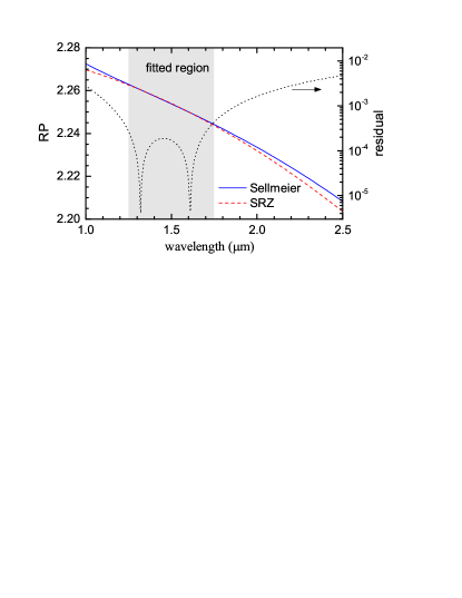
Figure 1: RP $\varepsilon_{\omega}$ of SCHOTT BK7 glass given by the Sellmeier expression Eq. (VI.2) (solid line), and fitted using a single resonance at zero frequency (dashed line). The absolute residual of the fit is given as dotted line.

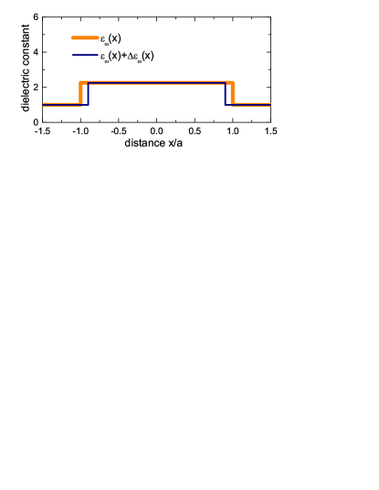
Figure 2: Cross-section of the perturbed and unperturbed wave guide used in Sec. VI.4 and Sec. VI.5, shown at a particular frequency.

VI.3 Unperturbed and perturbed system

The unperturbed system I consider in this work as example is a planar waveguide of width $2a=2\,\mu$m. I consider a size perturbation, narrowing the waveguide by $10$ percent, as shown in Fig. 2. For the in-plane wave vector component I have chosen $pa=5$. I choose as basis of size $N$ for the RSE all RSs with

$$|k_{n}\sqrt{\epsilon_{\omega_{n}}}|<k_{\rm max}(N)\,,$$ (56)

i.e., with a wave vector in the medium below a suitably chosen maximum $k_{\rm max}(N)$, this follows the approach of Ref.Egor .

The motivation for the choice of basis selection criteria is the analogy between the RSE and a Fourier expansion. As I increase $k_{n}\sqrt{\epsilon_{\omega_{n}}}$, I increase the number of oscillations in the field as can be seen from Eq. (43). These increasingly oscillating fields go into the basis and similar to Fourier series, increase the resolution of the composite field generated by the expansion.

VI.4 Single Sellmeier resonance at zero frequency

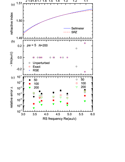
Figure 3: SRZ RSE results for a thickness perturbation of a planar waveguide as function of the real part of $\omega$. (a) Refractive index of the unperturbed and perturbed medium (dashed line) described by the SRZ Eq. (55) and of the BK7 Sellmeier dispersion (solid line) Eq. (VI.2). (b) RS frequencies for $N=200$. Shown are exact unperturbed (open circles), exact perturbed (open squares), and RSE perturbed (crosses) data. (c) Relative error $\Delta$ of the RSE perturbed RS frequencies for $N=50,100,200$. Closed symbols give relative error to the SRZ Eq. (55) RS eigen-frequencies as shown. Open symbols give relative error to the Sellmeier dispersion RS eigen-frequencies as shown. I show in (b) states with both incoming and outgoing boundary conditions, i.e. having positive or negative imaginary parts of complex resonant frequency, only states with outgoing boundary conditions go into the basis.

Here I show results of the SRZ yielding the linear eigenvalue problem Eq. (19). For the unperturbed and perturbed system I use a RP given by the SRZ Eq. (55). The refractive index of the unperturbed and perturbed system is compared in Fig. 3 with the Sellmeier expression Eq. (VI.2). I can see that for the chosen waveguide width, the fitted wavelength range corresponds to $3.6<a\omega/c<5$. The RS frequencies are given in Fig. 3(b) for the unperturbed system $\omega_{n}=c\sqrt{k_{n}^{2}+p^{2}}$ and for the perturbed system $\varpi_{\nu}=c\sqrt{\varkappa_{\nu}^{2}+p^{2}}$. To compare $\varpi_{\nu}$ calculated using the RSE with the exact result $\varpi_{\nu}^{\rm(exact)}$ obtained by the secular Eq. (44), I define the relative error $\Delta=\bigl{|}\varpi_{\nu}/\varpi_{\nu}^{\rm(exact)}-1\bigr{|}$, and give the resulting values in Fig. 3(c). I find that as I increase $N$, $\Delta$ decreases proportional to $N^{-3}$, similar to the findings for the non-dispersive RSE DoostPRA14 ; DoostPRA13 ; DoostPRA12 , and values in the $10^{-6}$ range are reached for $N=200$. This is actually smaller than the relative error due to the SRZ approximation of the Sellmeier dispersion (see Fig. 1).

Figure 4: SRZ RSE results for a thickness perturbation of a planar waveguide and $N=50$. Shown are $\Re(\omega_{\nu})$ as function of the in-plane wave vector $p$ with $\Im(\omega_{\nu})$ given by the color according to the scale shown.

The evolution of the perturbed RSs wavenumbers $\varpi_{\nu}$ with the in-plane wave vector $p$ is shown in Fig. 4. I can distinguish ArmitagePRA14 the waveguide (WG) and anti-waveguide (AWG) modes, which have real $\varpi_{\nu}$, and the Fabry-Pérot (FP) modes which have a finite imaginary part representing their losses. Increasing $p$, the FP modes split into WG and AWG mode at the bifurcation point at which $pc=\varpi_{\nu}$, at which $k=0$ i.e. at grazing incidence of the external field.

The relative error $\Delta$ of $\varpi_{\nu}$ is given in Fig. 5 as function of $p$. I can see that $\Delta$ has generally a weak dependence on $p$, except close to the bifurcation points, where the error of the FP and AWG mode is significantly increased. Under closer examination I see further smaller discontinuities as function of $p$, which correspond to a change of the basis states included according to Eq. (56) for fixed $N=50$. These results indicates that the RSE is able to reproduce all relevant RSs with a good accuracy.

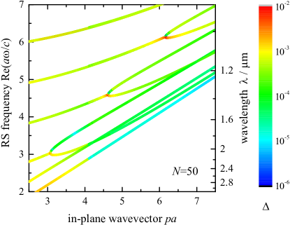
Figure 5: SRZ RSE results for a thickness perturbation of a planar waveguide and $N=50$. Shown are $\Re(\omega_{\nu})$ as function of the in-plane wave vector $p$ with the relative error $\Delta$ given by the color according to the scale shown.

VI.5 Sellmeier Dispersion

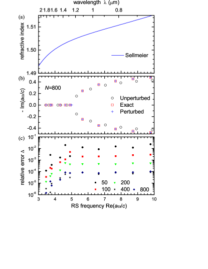
Figure 6: Sellmeier RSE results for a thickness perturbation of a planar waveguide. (a) refractive index of the Sellmeier dispersion given by Eq. (VI.2). (b) RS frequencies for $N=800$ basis states. Shown are exact unperturbed (open circles), exact perturbed (open squares), and RSE perturbed (crosses) data. (c) relative error $\Delta$ of the RSE perturbed RS frequencies $\varpi_{\nu}$ for $N=50,100,200,400,800$ basis states, as labeled. I show in (b) states with both incoming and outgoing boundary conditions, i.e. having positive or negative imaginary parts of complex resonant frequency, only states with out-going boundary conditions go into the basis.

Here I show results of the Sellmeier RSE yielding the quadratic eigenvalue problem Eq. (33).

The RS frequencies are given in Fig. 6(b) for the unperturbed system $\omega_{n}=c\sqrt{k_{n}^{2}+p^{2}}$ and for the perturbed system $\varpi_{\nu}=c\sqrt{\varkappa_{\nu}^{2}+p^{2}}$. The relative error $\Delta$ is given in Fig. 6(c). Also here I find that as we increase $N$, $\Delta$ decreases proportional to $N^{-3}$, and values in the $10^{-5}$ range are reached for $N=800$.

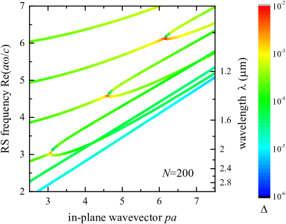
Figure 7: Sellmeier RSE results for a thickness perturbation of a planar waveguide and $N=200$. Shown are $\Re(\varpi_{\nu}$) as function of the in-plane wave vector $p$ with the relative error $\Delta$ given by the colour according to the scale shown.

The evolution of the perturbed RSs wavenumbers $\varpi_{\nu}$ with the in-plane wave vector $p$ is shown in Fig. 7 including the relative error $\Delta$, and in Fig. 4 including the imaginary part $\Im(\varpi_{\nu})$.

I can see that $\Delta$ has generally a weak dependence on $p$, except for the bifurcation points, at which a Fabry-Perot mode splits into a waveguide and anti-waveguide mode.

These results indicate that with full Sellmeier dispersion the RSE is able to reproduce all relevant RSs with a good accuracy.

VI.6 Performance Comparison

Here I compare the computational complexity of the SRZ RSE and the Sellmeier RSE. The corresponding eigenvalue problems Eq. (19) and Eq. (33) show that for the same number of basis states $N$, the SRZ RSE is a generalized eigenvalue problem of size $N\times N$, while the Sellmeier RSE has a size $2N\times 2N$ due to the quadratic nature of Eq. (33). Also I see from Fig. 8 that for $pa=5$ the resonances closely associated to the Sellmeier $\hat{q}_{j}$ poles, those eigen-frequencies found using the solutions to Eq. (76) as a starting point for the Newton-Raphson search, contribute approximately $10\%$ to the basis size thereby increasing the numerical complexity and reducing the efficiency.

In Fig. 9 I show a comparison between the average relative error in the perturbed resonances for $pa=5$ found in the range $3<a\omega<5$ versus the number of seconds required to diagonalise the perturbation eigenvalue problems using an Intel Core 2 Duo, 6M Cache, 3.16GHz, 1333MHz FSB processor connected to 4GB of RAM and using the NAG generalized eigenvalue problem solver software.

For the case of SRZ dispersion the relative error reaches the limit of about $5\times 10^{-5}$ due to the RP approximation at $N\approx 70$. Once the perturbation method using the full Sellmeier dispersion reaches this relative error I see that upon adding further basis states more noise in the relative error plot is generated and that the average relative error changes little. Fig. 9 suggests that the SRZ RSE is several orders of magnitude more efficient than the full Sellmeier RSE when considering the resonances over a small range of frequencies such as the small range used for optical communications.

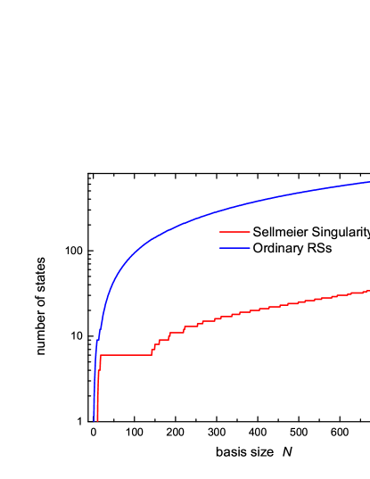
Figure 8: Graph showing quantitatively how the number of poles in the basis associated closely with the poles in the Sellmeier equation for $pa=5$, those eigenfrequencies found using the solutions to Eq. (76) as a starting point for the Newton-Raphson search, increase with basis size $N$ when the basis is selected according to Eq. (56). For reference I also show the number of ordinary poles, those found with the Newton-Raphson method without requiring the solutions of Eq. (76) as a starting point for their search and discovery, in the basis versus basis size $N$.

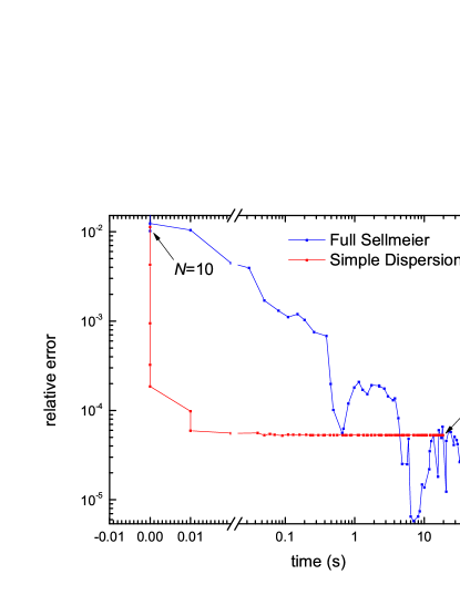
Figure 9: Comparison of the average relative error of the wave guide modes occurring in the range $3<a\omega<5$ calculated using the two different perturbation schemes in this paper versus time required to diagonalise the perturbation matrix using an Intel Core 2 Duo, 6M Cache, 3.16GHz, 1333MHz FSB processor connected to 4GB of RAM and using the NAG generalised eigenvalue problem solver software

VII RSE Born approximation for planar waveguides

In this section I derive the RSE Born approximation for planar waveguide, the equivalent theory for effectively 2D systems is given in Appendix G.

In effectively one dimension Eq. (2) becomes in free space (taking $c=1$),

$$\left[\nabla^{2}-\frac{1}{c^{2}}\frac{\partial^{2}}{\partial t^{2}}\right]\theta_{p}{E}({x})=0\,,$$ (57)

However, $\nabla^{2}\theta_{p}=-p^{2}\theta_{p}$, therefore

$$\left[\frac{d^{2}}{dx^{2}}+k^{2}\right]{E}({x})=0\,,$$ (58)

Hence the free space GF equation is,

$$\left[\frac{d^{2}}{dx^{2}}+k^{2}\right]G^{fs}_{k}(x,x^{\prime})=\delta(x-x^{\prime})\,,$$ (59)

which has the solution,

$$G^{fs}_{k}(x,x^{\prime})=-\dfrac{e^{ik|x-x^{\prime}|}}{2ik}$$ (60)

The systems associated with $G^{fs}_{k}$ and $G_{k}$ of Eq. (6) are related by the Dyson Equations perturbing back and forth with $\Delta\varepsilon_{\omega}(x)=\varepsilon_{\omega}(x)-1$ similar to Ref.Ge14 ,

$$G_{k}(x,x^{\prime\prime}) = G^{fs}_{k}(x,x^{\prime\prime})$$

$$-\omega^{2}\int G^{fs}_{k}(x,x^{\prime\prime\prime})\Delta\varepsilon_{\omega}(x^{\prime\prime\prime})G_{k}(x^{\prime\prime\prime},x^{\prime\prime})dx^{\prime\prime\prime}\,,$$

$$G_{k}(x^{\prime\prime\prime},x^{\prime\prime}) = G^{fs}_{k}(x^{\prime\prime\prime},x^{\prime\prime})$$

$$-\omega^{2}\int G_{k}(x^{\prime\prime\prime},x^{\prime})\Delta\varepsilon_{\omega}(x^{\prime})G^{fs}_{k}(x^{\prime},x^{\prime\prime})dx^{\prime}\,,$$

Combining Eq. (VII) and Eq. (VII) it is obtained similar to Ref.Ge14

$$G_{k}(x,x^{\prime\prime})=G^{fs}_{k}(x,x^{\prime\prime})\\ -\omega^{2}\int G^{fs}_{k}(x,x^{\prime})\Delta\varepsilon_{\omega}(x^{\prime})G^{fs}_{k}(x^{\prime},x^{\prime\prime})dx^{\prime}\\ +\omega^{4}\int\int G^{fs}_{k}(x,x^{\prime})\Delta\varepsilon_{\omega}(x^{\prime})G_{k}(x^{\prime},x^{\prime\prime\prime})\\ \times\Delta\varepsilon_{\omega}(x^{\prime\prime\prime})G^{fs}_{k}(x^{\prime\prime\prime},x^{\prime\prime})dx^{\prime\prime\prime}dx^{\prime}\,.$$ (63)

Hence, in one dimension the RSE Born approximation can be greatly simplified by using Eq. (60) and the spectral GF Eq. (109) in Eq. (63) to arrive at,

$$G_{k}(x,x^{\prime\prime})=-\dfrac{e^{ik(x^{\prime\prime}-x)}}{2ik}+\dfrac{\omega^{2}e^{ik(x^{\prime\prime}-x)}}{4k^{2}}\int_{-a}^{a}\Delta\varepsilon_{\omega}dx^{\prime}\\ -\dfrac{\omega^{4}e^{ik(x^{\prime\prime}-x)}}{4k^{2}}\sum_{n}\frac{A_{n}(x)A_{n}(x^{\prime\prime})}{2k(k-k_{n})}\,.$$ (64)

where $A_{n}$ is defined as the Fourier transform,

$$A_{n}(x)=\int_{-a}^{a}e^{ik\hat{x}x^{\prime}}\Delta\varepsilon_{\omega}(x^{\prime})E_{n}(x^{\prime})dx^{\prime}$$ (65)

Interestingly in one dimension I do not require the far field approximation to make the simplification of the Green’s function required to bring the RSE Born approximation to the form of Eq. (129). Hence, in one dimension the RSE Born Approximation is valid everywhere outside of the slab and not just in the far field. I note that fast Fourier transforms are available for use upon Eq. (65).

I demonstrate the computational accuracy of the RSE Born approximation in Fig. 10 where I calculate the transmission defined as

$$T(k,x^{\prime})=\left|2kG(x^{\prime},-a;k)\right|^{2}$$ (66)

For comparison the analytic GF is found by solving Maxwell’s wave equation in one dimension with a source of plane waves while making use of Maxwell’s boundary conditions. The system treated is the unperturbed system in Sec. VI.4 with $pa=5$.

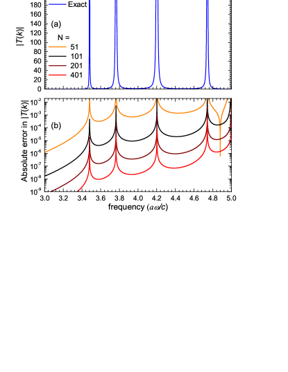
Figure 10: I give transmission results for the unperturbed system in Sec. VI.4 with $pa=5$. I have used analytic modes as RSs for the RSE Born approximation. (a) Exact transmission as a function of frequency as defined by Eq. (66) (b) Absolute error in transmission calculated using the analytic form of $T(k,x^{\prime})$ between $x=-a$ and $x=a$ versus frequency $\omega$ as comparison for the RSE Born approximation. Here $N=51,101,201,401$ as labeled.

From Fig. 10 we can see that unlike the standard Born approximation the RSE Born approximation is valid over an arbitrarily wide range of $k$ depending only on the basis size $N$ used. Furthermore we see that as the basis size increases the RSE Born approximation converges to the exact solution. The absolute error in the RSE Born approximation is approximately reduced by an order of magnitude each time the basis size is doubled. Absolute errors of $10^{-8}-10^{-5}$ are seen in the $k$ range shown for basis size $N=401$.

VIII Summary

In this work I have extended the RSE to media having a simple dispersion linear in wavelength squared. This dispersion has a single pole at zero frequency and does not introduce an additional dynamic degree of freedom as it would be the case for a more general Sellmeier model of the material response. This property allows to keep the simplicity of the RSE formulation, therefore retaining the advantage of the RSE in computational efficiency discussed in Ref. DoostPRA14, .

Furthermore, in this work I have also extended the RSE to waveguides obeying the Sellmeier equation for glasses. In order to do this I have reduced the order of the eigenvalue problem to second order by using sum rules as was done in Egor .

To make use of the RSs generated by the RSE I derived the RSE Born approximation for effectively 1D and 2D waveguides.

My conclusion is that the simple dispersion treatment is more efficient than using the full Sellmeier dispersion. This is because the dispersion only has to be correctly reproduced over a narrow part of the optical frequency range and therefore it is inefficient to include the full and at some frequencies unphysical Sellmeier dispersion.

Appendix A Sum rule

Here I use my approach of Ref.DoostARX15 , which was first adapted for full dispersion of 3D nano-particles by E. A. Muljarov in Ref.Egor , to derive sum rules and completeness of modes for the waveguide GF.

By substituting Eq. (5) into Eq. (6) and using Eq. (4) I have,

$$-\hat{\mathbf{1}}\delta(\mathbf{\dot{r}}-\mathbf{\dot{r}}^{\prime})=\sum_{n}{\dfrac{(\omega^{2}_{n}\hat{\boldsymbol{\varepsilon}}_{\omega_{n}}-\omega^{2}\hat{\boldsymbol{\varepsilon}}_{\omega})}{c^{2}2k_{n}(k-k_{n})}{\bf E_{n}}(\mathbf{\dot{r}})\otimes{\bf E_{n}}(\mathbf{\dot{r}}^{\prime})}\,.$$ (67)

I now consider the pole in $\hat{\boldsymbol{\varepsilon}}_{\omega}$ at $k=\pm\hat{q}_{j}$

$$\hat{\boldsymbol{\varepsilon}}_{\omega}=\dfrac{\hat{\boldsymbol{\sigma}}_{j}(\mathbf{\dot{r}})}{2k(k\pm\hat{q}_{j})}$$ (68)

where I have been able to ignored other terms in the dispersion since they are constant in the limit $k\rightarrow\mp\hat{q}_{j}$. Using $\omega^{2}/c^{2}=k^{2}+p^{2}$ and $\omega_{n}^{2}/c^{2}=k^{2}_{n}+p^{2}$ and Eq. (68) in Eq. (67), I find

$$=\dfrac{(\omega^{2}_{n}\hat{\boldsymbol{\varepsilon}}_{\omega_{n}}-\omega^{2}\hat{\boldsymbol{\varepsilon}}_{\omega})}{c^{2}2k_{n}(k-k_{n})}\\ ={2\hat{\boldsymbol{\sigma}}_{j}(\mathbf{\dot{r}})}\dfrac{kp^{2}}{8k^{2}_{n}k(k-k_{n})(k_{n}\pm\hat{q}_{j})}\\ -\dfrac{2\hat{\boldsymbol{\sigma}}_{j}(\mathbf{\dot{r}})}{(k\pm\hat{q}_{j})}\left(\dfrac{p^{2}k_{n}}{8k^{2}_{n}k(k-k_{n})}\pm\dfrac{k_{n}\hat{q}_{j}k}{8k^{2}_{n}k(k_{n}\pm\hat{q}_{j})}\right)$$ (69)

Then convoluting Eq. (67) with arbitrary finite function and taking the limit $k\rightarrow\mp\hat{q}_{j}$, I see that the second term is diverging unless

$$\sum_{n}\frac{{\bf E_{n}}(\mathbf{\dot{r}})\otimes{\bf E_{n}}(\mathbf{\dot{r}}^{\prime})}{k_{n}(k_{n}\pm\hat{q}_{j})}=0\,.$$ (70)

since when $k\rightarrow\mp\hat{q}_{j}$

$$\left(\dfrac{p^{2}k_{n}}{8k^{2}_{n}k(k-k_{n})}\pm\dfrac{k_{n}\hat{q}_{j}k}{8k^{2}_{n}k(k_{n}\pm\hat{q}_{j})}\right)\\ =\pm\dfrac{p^{2}+\hat{q}^{2}_{j}}{8k_{n}(k_{n}\pm\hat{q}_{j})\hat{q}_{j}}$$ (71)

The closure and over completeness follow from letting $\omega\rightarrow\infty$ to give DoostARX15

$$\dfrac{\hat{\boldsymbol{\varepsilon}}(\mathbf{\dot{r}})}{2}\sum_{n}\mathbf{E}_{n}(\mathbf{\dot{r}})\otimes\mathbf{E}_{n}(\mathbf{\dot{r}}^{\prime})=\hat{\mathbf{1}}\delta(\mathbf{\dot{r}}-\mathbf{\dot{r}}^{\prime})\,,$$ (72)

Appendix B Analytic solution of secular equation close to RP poles

Here I calculate an analytic approximation for the solutions of the secular equation Eq. (44) close to the poles of the RP, following the approach of Ref.Egor . In the limit $\epsilon_{\omega}\rightarrow\infty$ I find from Eq. (45) that $q_{n}\rightarrow\sqrt{\epsilon_{\omega}}\omega_{n}/c$, so that Eq. (44) is given by $-e^{iq_{n}a}+(-1)^{n}e^{-iq_{n}a}=0$, and thus

$$\begin{array}[]{lll}\sin(\sqrt{\epsilon_{\omega}}\omega_{n}a/c)=0&\mbox{for even}&n\\ \cos(\sqrt{\epsilon_{\omega}}\omega_{n}a/c)=0&\mbox{for odd}&n\end{array}$$ (73)

In the limit $k_{n}\rightarrow\pm\hat{q}_{j}$ to the poles of the RP given in Eq. (IV) I find

$$\epsilon_{\omega}\frac{\omega_{n}^{2}}{c^{2}}=\sigma_{j}\dfrac{k^{2}_{n}+p^{2}}{2k_{n}(k_{n}\mp\hat{q}_{j})}=\gamma_{n}$$ (74)

and solutions of Eq. (73) are given by

$$\gamma_{n}a^{2}=(\pi n/2)^{2}$$ (75)

The solutions of Eq. (74) with $k_{n}$ close to $\pm\hat{q}_{j}$ are given by the analytic solution of the quadratic formula

$$(\sigma_{j}-2\gamma_{n})k^{2}_{n}\pm 2\gamma_{n}\hat{q}_{j}k_{n}+\sigma_{j}p^{2}=0$$ (76)

I use the solutions of Eq. (76) as starting points for the Newton-Raphson search for RSs.

The RSs of the unperturbed system (see Sec. VI.3) with Sellmeier dispersion Eq. (VI.2) are given in Fig. 11. I note that close to the lowest resonance frequency of the dispersion at $\Omega_{j}a/c\approx 0.6174$, there are a large number of RSs approaching the pole from smaller frequencies. These RSs arise because the refractive index is diverging to positive infinity on the low frequency side, allowing for a countable infinite number of WG and AWG modes to form. $\sigma_{j}$ is negative for all the resonances in Eq. (VI.2).

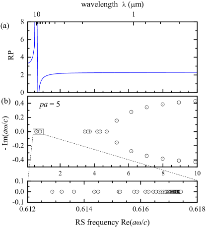
Figure 11: (a) RP as a function of frequency given by Eq. (VI.2). (b) Resonant frequencies $\omega_{n}$ of the homogeneous dielectric waveguide with $pa=5$ and this RP, forming the basis states for the Sellmeier RSE discussed in Sec. VI.5. (c) Zoom of (b) showing the series of poles on the low frequency side of the singularity in RP. I show in (b) and (c) states with both incoming and outgoing boundary conditions, i.e. having positive or negative imaginary parts of complex resonant frequency, only states with outgoing boundary conditions go into the basis.

Appendix C Calculation of L

Here I derive the form of the $L$ operator occurring in the reduced Maxwell’s wave equation for waveguide Eq. (4).

For planar systems $L$ is given in Ref. ArmitagePRA14, as

$$-L=\frac{d^{2}}{dx^{2}}-p^{2}$$ (77)

For effectively two-dimensional systems with one direction of translational invariance $L$ can be calculated as follows. Due to translational invariance in the direction $z$, the direction of propagation I can write the full field as,

$${\bf\hat{E}}({\bf r})=e^{ipz-i\omega t}{\bf E}(\mathbf{\dot{r}})=\theta_{p}{\bf E}(\mathbf{\dot{r}})\,,$$ (78)

where $\mathbf{\dot{r}}$ give the coordinates in the plane perpendicular to $z$.

Therefore using standard vector identities I can write

$$\nabla\times\nabla\times{\bf\hat{E}} = \nabla\times\nabla\times(\theta_{p}{\bf E})$$ (79)

$$= \nabla\times(\nabla\theta_{p}\times{\bf E}+\theta_{p}\nabla\times{\bf E})$$

$$= \nabla\theta_{p}(\nabla\cdot{\bf E})-{\bf E}(\nabla\cdot(\nabla\theta_{p}))$$

$$+({\bf E}\cdot\nabla)\nabla\theta_{p}-(\nabla\theta_{p}\cdot\nabla){\bf E}$$

$$+\nabla\theta_{p}\times\nabla\times{\bf E}$$

$$+\theta_{p}\nabla\times\nabla\times{\bf E}$$

I make use of the following identities,

$$\nabla\theta_{p} = ip\theta_{p}e_{z}$$ (80)

$$\nabla\cdot\nabla\theta_{p} = -p^{2}\theta_{p}$$ (81)

$$\nabla\theta_{p}(\nabla\cdot{\bf E}) = ip\theta_{p}(\nabla\cdot{\bf E})e_{z}$$ (82)

$$({\bf E}\cdot\nabla)\nabla\theta_{p} = (e_{z}\cdot{\bf E})p^{2}\theta_{p}e_{z}$$ (83)

$$\partial_{z}{\bf E} = 0$$ (84)

where $e_{z}$ is the unit vector in the $z$ direction so as to simplify Eq. (79) to

$$\nabla\times\nabla\times{\bf\hat{E}} = \nabla\times\nabla\times({\bf E}\theta_{p})$$

$$= ip\theta_{p}e_{z}(\nabla\cdot{\bf E})+{\bf E}p^{2}\theta_{p}$$

$$+(e_{z}\cdot{\bf E})p^{2}\theta_{p}e_{z}-ip\theta_{p}\partial_{z}{\bf E}$$

$$+ip\theta_{p}e_{z}\times\nabla\times{\bf E}+\theta_{p}\nabla\times\nabla\times{\bf E}$$

$$= \theta_{p}L({\bf E})$$

Hence I see that,

$$L({\bf E}) = ipe_{z}(\nabla\cdot{\bf E})+{\bf E}p^{2}$$

$$+(e_{z}\cdot{\bf E})p^{2}e_{z}+ipe_{z}\times\nabla\times{\bf E}$$

$$+\nabla\times\nabla\times{\bf E}$$

So $L$ is a linear operator independent of the RP and $z$ as required. Therefore the eigenvalue problems derived in Sec. III and Sec. IV are valid for planar and cylindrical wave guides. Also the derivation of $L$ demonstrates I can use separation of variables in Eq. (2) to arrive at Eq. (78).

Appendix D Spectral representation of the GF of an open system

Here I almost exactly repeat my derivations which I contributed to Ref.DoostPRA13 using exactly the same method but with increased mathematical rigour, in order to prove in this section the spectral representation of the Green’s function (GF) of a general wave equations.

The GF of an open waveguide equation system is a tensor function $\hat{\mathbf{G}}_{k}$ which satisfies the outgoing wave BCs and the waveguide wave equation Eq. (4) with a delta function source term,

$$-L\hat{\mathbf{G}}_{k}(\mathbf{\dot{r}},\mathbf{\dot{r}}^{\prime})+\hat{\boldsymbol{\varepsilon}}(\mathbf{\dot{r}},k)k^{2}\hat{\mathbf{G}}_{k}(\mathbf{\dot{r}},\mathbf{\dot{r}}^{\prime})=\hat{\mathbf{1}}\delta(\mathbf{\dot{r}}-\mathbf{\dot{r}}^{\prime})\,,$$ (87)

In this Appendix the effective permittivity $\hat{\boldsymbol{\varepsilon}}(\mathbf{\dot{r}},k)=\hat{\boldsymbol{\varepsilon}}_{\omega}(\mathbf{\dot{r}})(1+{p^{2}}/{k^{2}})$ with fixed $p$. Assuming a simple-pole structure of the GF inside the scatterer with poles at $k=q_{n}$ and taking into account its large-$k$ vanishing asymptotics, the Mittag-Leffler theorem allows us to express the GF only inside the scatterer as the convergent

$$\hat{\mathbf{G}}_{k}(\mathbf{\dot{r}},\mathbf{\dot{r}}^{\prime})=\sum_{n}\frac{\hat{\mathbf{Q}}_{n}(\mathbf{\dot{r}},\mathbf{\dot{r}}^{\prime})}{k-q_{n}}\,.$$ (88)

It will probably be that Eq. (88) will need to be experimentally verified by comparing scattering predicted by the RSE Born approximation with experimental results of scattering from well defined scatterers. It may be that Eq. (88) is a fundamental law of Physics. My justification for this form of the GF is the superposition of Lorentzians which make up the scattering profile of resonators and the numerical verification of this form of GF made in Ref.DoostPRA12 ; DoostPRA13 ; ArmitagePRA14 ; DoostPRA14 .

Assuming no degeneracy with the mode $n$, the definition of the residue tensor $\hat{\mathbf{Q}}_{n}(\mathbf{\dot{r}},\mathbf{\dot{r}}^{\prime})$ at a simple pole of the function $\hat{\mathbf{G}}_{k}(\mathbf{\dot{r}},\mathbf{\dot{r}}^{\prime})$ is,

$$\lim_{k\to q_{n}}(k-q_{n})\hat{\mathbf{G}}_{k}(\mathbf{\dot{r}},\mathbf{\dot{r}}^{\prime})=\hat{\mathbf{Q}}_{n}(\mathbf{\dot{r}},\mathbf{\dot{r}}^{\prime})$$ (89)

I have again assumed $\hat{\mathbf{G}}_{k}(\mathbf{\dot{r}},\mathbf{\dot{r}}^{\prime})$ to be holomorphic in this neighbourhood of $q_{n}$ except for at the poles $q_{n}$ so that it has a Laurent series at $q_{n}$. Substituting the expression Eq. (88) into Eq. (89) gives

$$\lim_{k\to q_{n}}(k-q_{n})\sum_{m}\frac{\hat{\mathbf{Q}}_{m}(\mathbf{\dot{r}},\mathbf{\dot{r}}^{\prime})}{k-q_{m}}=\hat{\mathbf{Q}}_{n}(\mathbf{\dot{r}},\mathbf{\dot{r}}^{\prime})$$ (90)

so that

$$\lim_{k\to q_{n}}(k-q_{n})\sum_{m\neq n}\frac{\hat{\mathbf{Q}}_{m}(\mathbf{\dot{r}},\mathbf{\dot{r}}^{\prime})}{k-q_{m}}=0$$ (91)

Substituting the expression Eq. (88) into Eq. (87) and convoluting with an arbitrary finite vector function ${\bf D}(\mathbf{\dot{r}})$ over a finite volume $V$ we obtain

$$\sum_{n}\frac{-L\mathbf{F}_{n}({\mathbf{\dot{r}}})+\hat{\boldsymbol{\varepsilon}}(\mathbf{\dot{r}},k)k^{2}\mathbf{F}_{n}(\mathbf{\dot{r}})}{k-q_{n}}={\bf D}(\mathbf{\dot{r}})\,,$$ (92)

where $\mathbf{F}_{n}(\mathbf{\dot{r}})=\int_{V}\hat{\mathbf{Q}}_{n}(\mathbf{\dot{r}},\mathbf{\dot{r}}^{\prime}){\bf D}(\mathbf{\dot{r}}^{\prime})d\mathbf{\dot{r}}^{\prime}$. Multiplying by $(k-q_{n})$ and taking the limit $k\to q_{n}$ yields

$$\lim_{k\to q_{n}}(k-q_{n})\sum_{m}\frac{-L\mathbf{F}_{m}({\mathbf{\dot{r}}})+\hat{\boldsymbol{\varepsilon}}(\mathbf{\dot{r}},k)k^{2}\mathbf{F}_{m}(\mathbf{\dot{r}})}{k-q_{m}}$$ (93)

$$=\lim_{k\to q_{n}}(k-q_{n}){\bf D}(\mathbf{\dot{r}})=0\,.$$ (94)

From Eq. (91) we can see,

$$\lim_{k\to q_{n}}(k-q_{n})\sum_{m\neq n}\frac{-L\mathbf{F}_{m}({\mathbf{\dot{r}}})+\hat{\boldsymbol{\varepsilon}}(\mathbf{\dot{r}},k)k^{2}\mathbf{F}_{m}(\mathbf{\dot{r}})}{k-q_{m}}=0\,,$$ (95)

so we can drop terms $n\neq m$ from the summation in Eq. (94) to give

$$\lim_{k\to q_{n}}(k-q_{n})\dfrac{-L\mathbf{F}_{n}(\mathbf{\dot{r}})+\hat{\boldsymbol{\varepsilon}}(\mathbf{\dot{r}},k)k^{2}\mathbf{F}_{n}(\mathbf{\dot{r}})}{k-q_{n}}=0\,.$$ (96)

or

$$-L\mathbf{F}_{n}(\mathbf{\dot{r}})+\hat{\boldsymbol{\varepsilon}}(\mathbf{\dot{r}},q_{n})q^{2}_{n}\mathbf{F}_{n}(\mathbf{\dot{r}})=0\,.$$ (97)

Due to the convolution with the GF, $\mathbf{F}_{n}(\mathbf{\dot{r}})$ satisfies the same outgoing wave BCs. Then, according to Eq. (4), $\mathbf{F}_{n}(\mathbf{\dot{r}})\propto\mathbf{E}_{n}(\mathbf{\dot{r}})$ and $q_{n}=k_{n}$, i.e.

$$L\mathbf{E}_{n}(\mathbf{\dot{r}})=\hat{\boldsymbol{\varepsilon}}(\mathbf{\dot{r}},k_{n})k^{2}_{n}\mathbf{E}_{n}(\mathbf{\dot{r}})\,,$$ (98)

Note that the convolution of the kernel $\hat{\mathbf{Q}}_{n}(\mathbf{\dot{r}},\mathbf{\dot{r}}^{\prime})$ with different vector functions $\bf D(\mathbf{\dot{r}})$ can be proportional to one and the same vector function $\mathbf{E}_{n}(\mathbf{\dot{r}})$ only if the kernel has the form of a product:

$$\hat{\mathbf{Q}}_{n}(\mathbf{\dot{r}},\mathbf{\dot{r}}^{\prime})=\mathbf{E}_{n}(\mathbf{\dot{r}})\otimes\mathbf{E}_{n}(\mathbf{\dot{r}}^{\prime})/2k_{n}\,,$$ (99)

where $\otimes$ is the dyadic product operator.

The symmetry in Eq. (99) follows from the reciprocity theorem, described mathematically by the relation

$${\bf s}_{1}\hat{\mathbf{G}}_{k}(\mathbf{\dot{r}}_{1},\mathbf{\dot{r}}_{2}){\bf s}_{2}={s}_{2}\hat{\mathbf{G}}_{k}(\mathbf{\dot{r}}_{2},\mathbf{\dot{r}}_{1}){s}_{1}\,,$$ (100)

which holds for any two point sources ${s}_{1,2}$ at points $\mathbf{\dot{r}}_{1,2}$ emitting at the same frequency. Hence $\hat{\mathbf{G}}_{k}(\mathbf{\dot{r}},\mathbf{\dot{r}}^{\prime})$ is symmetric.

In the case of a GF made up of degenerate modes the proof of Eq. (99) is modified by making use of orthogonality of the degenerate modes to choose ${\bf D}({\mathbf{\dot{r}}})$ such that,

$$\int_{V}\mathbf{E}_{m}(\mathbf{\dot{r}})\cdot{\bf D}({\mathbf{\dot{r}}})\,d\mathbf{\dot{r}}=0\,,$$ (101)

for $m\neq n$ and where state $m$ is degenerate with $n$.

Hence I obtain

$$\hat{\mathbf{G}}_{k}(\mathbf{\dot{r}},\mathbf{\dot{r}}^{\prime})=\sum_{n}\frac{\mathbf{E}_{n}(\mathbf{\dot{r}})\otimes\mathbf{E}_{n}(\mathbf{\dot{r}}^{\prime})}{2k_{n}(k-k_{n})}\,.$$ (102)

Appendix E Derivation of sum rule and completeness

Here I exactly repeat my derivation of the sum rule and completeness of the GF which I made for Ref.DoostARX15 but in more detail.

In order to simplify the RSE Born approximation we require an appropriate spectral form of the GF which is different from the one already proven in Appendix D. To obtain this correct form I start with the GF valid inside the scatterer only,

$$\hat{\mathbf{G}}_{k}(\mathbf{\dot{r}},\mathbf{\dot{r}}^{\prime})=\sum_{n}\frac{\mathbf{E}_{n}(\mathbf{\dot{r}})\otimes\mathbf{E}_{n}(\mathbf{\dot{r}}^{\prime})}{2k_{n}(k-k_{n})}\,.$$ (103)

Substituting Eq. (103) in

$$-L\hat{\mathbf{G}}_{k}(\mathbf{\dot{r}},\mathbf{\dot{r}}^{\prime})+(k^{2}+p^{2})\hat{\boldsymbol{\varepsilon}}_{\omega}(\mathbf{\dot{r}})\hat{\mathbf{G}}_{k}(\mathbf{\dot{r}},\mathbf{\dot{r}}^{\prime})=\hat{\mathbf{1}}\delta(\mathbf{\dot{r}}-\mathbf{\dot{r}}^{\prime})\,,$$ (104)

gives for $k\to\infty$,

$$\hat{\boldsymbol{\varepsilon}}(\mathbf{\dot{r}})\sum_{n}\dfrac{(k+k_{n})\mathbf{E}_{n}(\mathbf{\dot{r}})\otimes\mathbf{E}_{n}(\mathbf{\dot{r}}^{\prime})}{2k_{n}}=\hat{\mathbf{1}}\delta(\mathbf{\dot{r}}-\mathbf{\dot{r}}^{\prime})\,.$$ (105)

since throughout the derivation in this appendix we are considering the limit where $k\to\infty$ at which $\hat{\boldsymbol{\varepsilon}}_{k}(\mathbf{\dot{r}})=\hat{\boldsymbol{\varepsilon}}(\mathbf{\dot{r}})$, i.e. the system is non-dispersive at high frequencies.

Convoluting Eq. (105) with arbitrary finite functions ${\bf D}$ which are only non-zero inside the resonator, gives

$$\int\left(\hat{\boldsymbol{\varepsilon}}(\mathbf{\dot{r}})\sum_{n}\dfrac{(k+k_{n})\mathbf{E}_{n}(\mathbf{\dot{r}})\otimes\mathbf{E}_{n}(\mathbf{\dot{r}}^{\prime})}{2k_{n}}\right){\bf D}(\mathbf{\dot{r}}^{\prime})d\mathbf{\dot{r}}^{\prime}={\bf D}(\mathbf{\dot{r}})\,.$$ (106)

and assuming the series are convergent as $k\rightarrow\infty$ we get,

$$\int\left(\sum_{n}\dfrac{\mathbf{E}_{n}(\mathbf{\dot{r}})\otimes\mathbf{E}_{n}(\mathbf{\dot{r}}^{\prime})}{2k_{n}}\right){\bf D}(\mathbf{\dot{r}}^{\prime})d\mathbf{\dot{r}}^{\prime}=0\,.$$ (107)

and since this is true for all ${\bf D}$ it follows that

$$\sum_{n}\dfrac{\mathbf{E}_{n}(\mathbf{\dot{r}})\otimes\mathbf{E}_{n}(\mathbf{\dot{r}}^{\prime})}{2k_{n}}=0\,.$$ (108)

Combining Eq. (103) and Eq. (108) yields

$$\hat{\mathbf{G}}_{k}(\mathbf{\dot{r}},\mathbf{\dot{r}}^{\prime})=\sum_{n}\frac{\mathbf{E}_{n}(\mathbf{\dot{r}})\otimes\mathbf{E}_{n}(\mathbf{\dot{r}}^{\prime})}{2k(k-k_{n})}\,.$$ (109)

Combining Eq. (105) and Eq. (108) leads to the closure relation

$$\dfrac{\hat{\boldsymbol{\varepsilon}}(\mathbf{\dot{r}})}{2}\sum_{n}\mathbf{E}_{n}(\mathbf{\dot{r}})\otimes\mathbf{E}_{n}(\mathbf{\dot{r}}^{\prime})=\hat{\mathbf{1}}\delta(\mathbf{\dot{r}}-\mathbf{\dot{r}}^{\prime})\,,$$ (110)

which expresses the completeness of the RSs, so that any function can be written as a superposition of RSs. If in the perturbed system some of the series are not convergent or are instead conditionally convergent then we will not arrive at the sum rule and completeness, in which case I expect that the RSE Born approximation will still give convergence to the exact solution but only if a valid spectral Green’s function is used, such as Eq. (103).

Appendix F Derivation of the correct normalisation for effectively 2D waveguides

Here I almost exactly repeat my derivations which I contributed to Ref.DoostPRA14 using exactly the same method as for Maxwell’s equations in order to prove in this section that the spectral representation, only valid inside the waveguide (similar to Ref.DoostARX15 for nano-particles), rigorously derived in Appendix C, D, and E

$$\hat{\mathbf{G}}_{k}(\mathbf{\dot{r}},\mathbf{\dot{r}}^{\prime})=\sum_{n}\frac{\mathbf{E}_{n}(\mathbf{\dot{r}})\otimes\mathbf{E}_{n}(\mathbf{\dot{r}}^{\prime})}{2k(k-k_{n})}\,,$$ (111)

leads to the RS normalization condition Eq. (F) for general waveguide equations. To do so, I consider an analytic continuation $\mathbf{E}(\mathbf{\dot{r}},k)$ of the vector wave function $\mathbf{E}_{n}(\mathbf{\dot{r}})$ around the point $k=k_{n}$ in the complex $k$-plane ($k_{n}$ is the wavenumber of the given RS). I select the analytic continuation such that it satisfies the outgoing wave boundary condition and my waveguide equation (taking $c=1$)

$$-L\mathbf{E}(\mathbf{\dot{r}},k)+\hat{\boldsymbol{\varepsilon}}(\mathbf{\dot{r}},\omega)(k^{2}+p^{2})\mathbf{E}(\mathbf{\dot{r}},k)=(k^{2}-k_{n}^{2})\boldsymbol{\sigma}(\mathbf{\dot{r}})$$ (112)

with an arbitrary source term.

The source $\boldsymbol{\sigma}(\mathbf{\dot{r}})$ has to be zero outside the cross-section of the inhomogeneity of $\hat{\boldsymbol{\varepsilon}}_{\omega}(\mathbf{\dot{r}})$ for the field $\mathbf{E}(\mathbf{\dot{r}},k)$ to satisfy the outgoing wave boundary condition. It also has to be non-zero somewhere inside that cross-section, as otherwise $\mathbf{E}(\mathbf{\dot{r}},k)$ would be identical to $\mathbf{E}_{n}(\mathbf{\dot{r}})$. It is further require that $\boldsymbol{\sigma}(\mathbf{\dot{r}})$ is normalized according to

$$\int_{A}\mathbf{E}_{n}(\mathbf{\dot{r}})\cdot\boldsymbol{\sigma}(\mathbf{\dot{r}})\,d\mathbf{\dot{r}}=1+\delta_{k_{n},0}\,,$$ (113)

The integral in Eq. (113) is taken over an arbitrary cross-section $A$ which includes all system inhomogeneity of $\hat{\boldsymbol{\varepsilon}}_{\omega}({\mathbf{\dot{r}}})$. I do not derive Eq. (113), it is simply a convenient condition to put on the otherwise arbitrary spatial dependence of the source which lies only inside the waveguide scatterer. If I had made the condition anything else (which in my earliest proof I did) then algebra and cancellation would lead us back to the same result, however with more mathematical complexity and operations. The condition make the mathematics easier because it causes $\mathbf{E}\rightarrow\mathbf{E}_{n}$ exactly and without proportionality constant appearing, equation (113) ensures that the analytic continuation reproduces $\mathbf{E}_{n}(\mathbf{\dot{r}})$ in the limit $k\to k_{n}$. Solving Eq. (112) with the help of the GF and using its spectral representation Eq. (111), I find:

$$\!\!\!\!\!\!\!\!\!\!\!\!\!\!\!\!\!\!\mathbf{E}(\mathbf{\dot{r}},k)=\int_{A}\hat{\mathbf{G}}_{k}(\mathbf{\dot{r}},\mathbf{\dot{r}}^{\prime})(k^{2}-k_{n}^{2})\boldsymbol{\sigma}(\mathbf{\dot{r}}^{\prime})d\mathbf{\dot{r}}^{\prime}$$

$$\!\!\!\!\!\!\!=\sum_{m}\mathbf{E}_{m}(\mathbf{\dot{r}})\frac{k^{2}-k_{n}^{2}}{2k(k-k_{m})}\int_{A}\mathbf{E}_{m}(\mathbf{\dot{r}}^{\prime})\cdot\boldsymbol{\sigma}(\mathbf{\dot{r}}^{\prime})\,d\mathbf{\dot{r}}^{\prime},$$ (114)

and then, using Eq. (113), obtain

$$\lim_{k\to{k_{n}}}\mathbf{E}(\mathbf{\dot{r}},k)=\mathbf{E}_{n}(\mathbf{\dot{r}})\,,$$

for any $\mathbf{\dot{r}}$ inside the system. Outside the system, the analytic continuation $\mathbf{E}(\mathbf{\dot{r}},k)$ is defined as a solution of the waveguide equation wave equation in free space. This solution is connected to the field inside the system [given by Eq. (114)] through the boundary conditions. Note that in the case of degenerate modes, $k_{m}=k_{n}$ for $m\neq n$, the current $\boldsymbol{\sigma}(\mathbf{\dot{r}})$ has to be chosen in such a way that it satisfies Eq. (113) and, additionally,

$$\int_{A}{\mathbf{E}_{m}}(\mathbf{\dot{r}})\cdot\boldsymbol{\sigma}(\mathbf{\dot{r}})\,d\mathbf{\dot{r}}=0\,,$$

in order that the degenerate modes can be normalised separately.

I now consider the integral

$$I_{n}(k)=\frac{\int_{A}(\mathbf{E}\cdot L\mathbf{E}_{n}-\mathbf{E}_{n}\cdot L\mathbf{E})d\mathbf{\dot{r}}}{k^{2}-k_{n}^{2}}$$ (115)

and evaluate it by using the waveguide equations Eqs. (4) and (112) for $\mathbf{E}_{n}$ and $\mathbf{E}$, respectively, and the source term normalization Eq. (113):

$$I_{n}(k)=\frac{\int_{A}(\mathbf{E}\cdot\omega_{n}^{2}\hat{\boldsymbol{\varepsilon}}_{\omega_{n}}\mathbf{E}_{n}-\mathbf{E}_{n}\cdot\omega^{2}\hat{\boldsymbol{\varepsilon}}_{\omega}\mathbf{E})d\mathbf{\dot{r}}}{k^{2}-k_{n}^{2}}+1+\delta_{k_{n},0}\,,$$ (116)

where I assume that $\hat{\boldsymbol{\varepsilon}}_{\omega}$ is a a (real) symmetric matrix or a scalar so that (defined to be in this case) $\mathbf{E}\cdot\hat{\boldsymbol{\varepsilon}}_{\omega_{n}}\mathbf{E}_{n}=\mathbf{E}_{n}\cdot\hat{\boldsymbol{\varepsilon}}_{\omega_{n}}\mathbf{E}$, and so I obtain also by commutation of $\mathbf{E}$ and $\mathbf{E}_{n}$ and simple calculus in the integral shown Eq. (116) the dispersion factor and normalization becomes,

$$1+\delta_{k_{n},0} = \int_{A}{\bf E_{n}}(\mathbf{\dot{r}})\cdot\dfrac{\partial(\omega^{2}\hat{\boldsymbol{\varepsilon}}_{\omega}(\mathbf{\dot{r}}))}{\partial(\omega^{2})}\biggr{\rvert}_{\omega=\omega_{n}}\!\!{\bf E_{n}}(\mathbf{\dot{r}})d{\mathbf{\dot{r}}}$$

$$+\lim_{k\rightarrow k_{n}}\int_{A}\dfrac{{\bf E_{n}(\mathbf{\dot{r}})}L{\bf\mathbf{E}(\mathbf{\dot{r}},k)}-{\bf\mathbf{E}(\mathbf{\dot{r}},k)}L{\bf E_{n}(\mathbf{\dot{r}})}}{k^{2}-k^{2}_{n}}d{\mathbf{\dot{r}}}$$

and then finally with $L_{A}$ the circumference of $A$,

$$1+\delta_{k_{n},0} = \int_{A}\mathbf{E}_{n}(\mathbf{\dot{r}})\cdot\dfrac{\partial\omega^{2}\hat{\boldsymbol{\varepsilon}}(\mathbf{\dot{r}},\omega)}{\partial\omega^{2}}\bigg{|}_{\omega=\omega_{n}}\!\!\mathbf{E}_{n}(\mathbf{\dot{r}})d{\mathbf{\dot{r}}}$$

$$+\lim_{k\rightarrow k_{n}}\oint_{L_{A}}\dfrac{\mathbf{E}_{n}\cdot\nabla\mathbf{E}-\mathbf{E}\cdot\nabla\mathbf{E}_{n}}{k^{2}-k^{2}_{n}}d{\bf L}\,.$$

I have also assumed a simpler form for the waveguide equation in free space, see Appendix G so that I can use the vector and scalar Green’s theorem to simplify Eq. (F). Various schemes exist to evaluate the line integral limit in Eq. (F) such as analytic methods in Ref.MuljarovEPL10 or numerically extending the closed arc into a non-reflecting, absorbing, perfectly matched layer where it vanishes.

Due to the over completeness of the basis demonstrated in Appendix E we do not have the relation we find for Hermitian systems

$$\int_{\it allspace}\dfrac{\omega^{2}_{n}\hat{\boldsymbol{\varepsilon}}_{\omega_{n}}(\mathbf{\dot{r}})-\omega^{2}_{m}\hat{\boldsymbol{\varepsilon}}_{\omega_{m}}(\mathbf{\dot{r}})}{\omega^{2}_{m}-\omega^{2}_{n}}{\mathbf{E}_{m}}(\mathbf{\dot{r}})\cdot{\mathbf{E}_{n}}(\mathbf{\dot{r}})\,d\mathbf{\dot{r}}=0\,,$$ (119)

for all $m\neq n$. The basis states of non-Hermitian systems are not all mutually orthogonal although some are orthogonal to one another. Hence we cannot derive for non-Hermitian systems the normalization relation, which is well known for Hermitian systems and follows from Eq. (119),

$$\int_{\it allspace}\dfrac{\partial(\omega^{2}\hat{\boldsymbol{\varepsilon}}_{\omega}(\mathbf{\dot{r}}))}{\partial(\omega^{2})}\biggr{\rvert}_{\omega=\omega_{n}}\!\!{\mathbf{E}_{n}}(\mathbf{\dot{r}})\cdot{\mathbf{E}_{n}}(\mathbf{\dot{r}})\,d\mathbf{\dot{r}}=1+\delta_{k_{n},0}\,,$$ (120)

and, hence, Eq. (F) and Eq. (120) are different.

Appendix G RSE Born Approximation for effectively 2D waveguides

In effectively two dimensions Eq. (2) becomes in free space (taking $c=1$),

$$\left[\nabla^{2}-\frac{1}{c^{2}}\frac{\partial^{2}}{\partial t^{2}}\right]\theta_{p}{\bf E}(\mathbf{\dot{r}})=0\,,$$ (121)

However $\nabla^{2}\theta_{p}=-p^{2}\theta_{p}$, therefore

$$\left[\nabla^{2}+k^{2}\right]{\bf E}=0\,,$$ (122)

Hence the free space GF equation is,

$$\left[\nabla^{2}+k^{2}\right]\hat{\mathbf{G}}^{fs}_{k}(\mathbf{\dot{r}},\mathbf{\dot{r}}^{\prime})=\hat{\mathbf{1}}\delta(\mathbf{\dot{r}}-\mathbf{\dot{r}}^{\prime})\,,$$ (123)

which has the solution, also assuming $\rho>>\rho^{\prime}$,

$$\hat{\mathbf{G}}^{fs}_{k}(\mathbf{\dot{r}},\mathbf{\dot{r}}^{\prime})=-\dfrac{i}{4}H_{0}(k|\mathbf{\dot{r}}-\mathbf{\dot{r}}^{\prime}|)\hat{\mathbf{1}}\approx Q\sqrt{\dfrac{1}{\rho\pi}}e^{ik|\mathbf{\dot{r}}-\mathbf{\dot{r}}^{\prime}|}\hat{\mathbf{1}}$$ (124)

The systems associated with $G^{fs}_{k}$ and $G_{k}$ of Eq. (6) are related by the Dyson Equations perturbing back and forth with $\Delta\hat{\boldsymbol{\varepsilon}}_{\omega}(\mathbf{\dot{r}})=\hat{\boldsymbol{\varepsilon}}_{\omega}(\mathbf{\dot{r}})-\hat{\mathbf{1}}$ similar to Ref.Ge14 ,

$$\hat{\mathbf{G}}_{k}(\mathbf{\dot{r}},\mathbf{\dot{r}}^{\prime\prime}) = \hat{\mathbf{G}}^{fs}_{k}(\mathbf{\dot{r}},\mathbf{\dot{r}}^{\prime\prime})$$

$$-\omega^{2}\int\hat{\mathbf{G}}^{fs}_{k}(\mathbf{\dot{r}},\mathbf{\dot{r}}^{\prime\prime\prime})\Delta\hat{\boldsymbol{\varepsilon}}_{\omega}(\mathbf{\dot{r}}^{\prime\prime\prime})\hat{\mathbf{G}}_{k}(\mathbf{\dot{r}}^{\prime\prime\prime},\mathbf{\dot{r}}^{\prime\prime})d\mathbf{\dot{r}}^{\prime\prime\prime}\,,$$

$$\hat{\mathbf{G}}_{k}(\mathbf{\dot{r}}^{\prime\prime\prime},\mathbf{\dot{r}}^{\prime\prime}) = \hat{\mathbf{G}}^{fs}_{k}(\mathbf{\dot{r}}^{\prime\prime\prime},\mathbf{\dot{r}}^{\prime\prime})$$

$$-\omega^{2}\int\hat{\mathbf{G}}_{k}(\mathbf{\dot{r}}^{\prime\prime\prime},\mathbf{\dot{r}}^{\prime})\Delta\hat{\boldsymbol{\varepsilon}}_{\omega}(\mathbf{r}^{\prime})\hat{\mathbf{G}}^{fs}_{k}(\mathbf{\dot{r}}^{\prime},\mathbf{\dot{r}}^{\prime\prime})d\mathbf{\dot{r}}^{\prime}\,,$$

Combining Eq. (G) and Eq. (G) it is obtained similar to Ref.Ge14

$$\hat{\mathbf{G}}_{k}(\mathbf{\dot{r}},\mathbf{\dot{r}}^{\prime\prime})=\hat{\mathbf{G}}^{fs}_{k}(\mathbf{\dot{r}},\mathbf{\dot{r}}^{\prime\prime})\\ -\omega^{2}\int\hat{\mathbf{G}}^{fs}_{k}(\mathbf{\dot{r}},\mathbf{\dot{r}}^{\prime})\Delta\hat{\boldsymbol{\varepsilon}}_{\omega}(\mathbf{\dot{r}}^{\prime})\hat{\mathbf{G}}^{fs}_{k}(\mathbf{\dot{r}}^{\prime},\mathbf{\dot{r}}^{\prime\prime})d\mathbf{\dot{r}}^{\prime}\\ +\omega^{4}\int\int\hat{\mathbf{G}}^{fs}_{k}(\mathbf{\dot{r}},\mathbf{\dot{r}}^{\prime})\Delta\hat{\boldsymbol{\varepsilon}}_{\omega}(\mathbf{\dot{r}}^{\prime})\hat{\mathbf{G}}_{k}(\mathbf{\dot{r}}^{\prime},\mathbf{\dot{r}}^{\prime\prime\prime})\\ \times\Delta\hat{\boldsymbol{\varepsilon}}_{\omega}(\mathbf{\dot{r}}^{\prime\prime\prime})\hat{\mathbf{G}}^{fs}_{k}(\mathbf{\dot{r}}^{\prime\prime\prime},\mathbf{\dot{r}}^{\prime\prime})d\mathbf{\dot{r}}^{\prime\prime\prime}d\mathbf{\dot{r}}^{\prime}\,.$$ (127)

In order to improve the numerical performance further I make a final few steps as in the original Born approximation Born26 , I define unit vector $\hat{\mathbf{\dot{r}}}$ such that $\mathbf{\dot{r}}=\rho\hat{\mathbf{\dot{r}}}$ and $\mathbf{k}_{s}=k\hat{\mathbf{\dot{r}}}$. Then for $\rho>>\rho^{\prime}$,

$$k|\mathbf{\dot{r}}-\mathbf{\dot{r}}^{\prime}|=k\rho-\mathbf{k}_{s}\cdot\mathbf{\dot{r}}^{\prime}+{\it O}\left(\dfrac{1}{\rho^{2}}\right)+...$$ (128)

Therefore substituting Eq. (5) and Eq. (124) in to Eq. (127) and using Eq. (128) because both $\mathbf{\dot{r}},\mathbf{\dot{r}}^{\prime\prime}$ are far from the scatterer I arrive at the RSE Born approximation

$$\hat{\mathbf{G}}_{k}(\mathbf{\dot{r}},\mathbf{\dot{r}}^{\prime\prime})=-\dfrac{i}{4}H_{0}(k|\mathbf{\dot{r}}-\mathbf{\dot{r}}^{\prime\prime}|)\hat{\mathbf{1}}\\ -\omega^{2}\dfrac{Q^{2}e^{ik(\rho+\rho^{\prime\prime})}}{\pi\sqrt{\rho\rho^{\prime\prime}}}\int e^{i(\mathbf{k}_{s}-\mathbf{k}_{s}^{\prime\prime})\cdot\mathbf{\dot{r}}^{\prime}}\Delta\hat{\boldsymbol{\varepsilon}}_{\omega}(\mathbf{\dot{r}}^{\prime})d\mathbf{\dot{r}}^{\prime}\\ +\omega^{4}\dfrac{Q^{2}e^{ik(\rho+\rho^{\prime\prime})}}{\pi\sqrt{\rho\rho^{\prime\prime}}}\sum_{n}\frac{\mathbf{A}_{n}({\mathbf{k}_{s}})\otimes\mathbf{A}_{n}(-{\mathbf{k}_{s}}^{\prime\prime})}{2k(k-k_{n})}\,.$$ (129)

or using Eq. (103) instead

$$\hat{\mathbf{G}}_{k}(\mathbf{\dot{r}},\mathbf{\dot{r}}^{\prime\prime})=-\dfrac{i}{4}H_{0}(k|\mathbf{\dot{r}}-\mathbf{\dot{r}}^{\prime\prime}|)\hat{\mathbf{1}}\\ -\omega^{2}\dfrac{Q^{2}e^{ik(\rho+\rho^{\prime\prime})}}{\pi\sqrt{\rho\rho^{\prime\prime}}}\int e^{i(\mathbf{k}_{s}-\mathbf{k}_{s}^{\prime\prime})\cdot\mathbf{\dot{r}}^{\prime}}\Delta\hat{\boldsymbol{\varepsilon}}_{\omega}(\mathbf{\dot{r}}^{\prime})d\mathbf{\dot{r}}^{\prime}\\ +\omega^{4}\dfrac{Q^{2}e^{ik(\rho+\rho^{\prime\prime})}}{\pi\sqrt{\rho\rho^{\prime\prime}}}\sum_{n}\frac{\mathbf{A}_{n}({\mathbf{k}_{s}})\otimes\mathbf{A}_{n}(-{\mathbf{k}_{s}}^{\prime\prime})}{2k_{n}(k-k_{n})}\,.$$ (130)

The vector $\mathbf{A}_{n}$ is defined as a Fourier transform of the RSs,

$$\mathbf{A}_{n}(\mathbf{k}_{s})=\int e^{i\mathbf{k}_{s}\cdot\mathbf{\dot{r}}^{\prime}}\Delta\hat{\boldsymbol{\varepsilon}}_{\omega}(\mathbf{\dot{r}}^{\prime})\mathbf{E}_{n}(\mathbf{\dot{r}}^{\prime})d\mathbf{\dot{r}}^{\prime}$$ (131)

I note that the fast Fourier transform method is available. The first two terms in Eq. (129) correspond to the standard Born approximation, the final summation term corresponds to the RSE correction to the Born approximation.

A simple corollary of this theory is as follows, I can see from the arguments just stated that from Eq.(G5) if $\mathbf{\dot{r}}^{\prime\prime}$ is inside the resonator and $\rho>>\rho^{\prime\prime}$ then

$$\hat{\mathbf{G}}_{k}(\mathbf{\dot{r}},\mathbf{\dot{r}}^{\prime\prime})=-\dfrac{i}{4}H_{0}(k|\mathbf{\dot{r}}-\mathbf{\dot{r}}^{\prime\prime}|)\hat{\mathbf{1}}\\ -\omega^{2}\dfrac{Qe^{ik\rho}}{\sqrt{\rho\pi}}\sum_{n}\frac{\mathbf{A}_{n}({\mathbf{k}_{s}})\otimes\mathbf{E}_{n}({\mathbf{\dot{r}}}^{\prime\prime})}{2k(k-k_{n})}\,,$$ (132)

or using Eq. (103) instead

$$\hat{\mathbf{G}}_{k}(\mathbf{\dot{r}},\mathbf{\dot{r}}^{\prime\prime})=-\dfrac{i}{4}H_{0}(k|\mathbf{\dot{r}}-\mathbf{\dot{r}}^{\prime\prime}|)\hat{\mathbf{1}}\\ -\omega^{2}\dfrac{Qe^{ik\rho}}{\sqrt{\rho\pi}}\sum_{n}\frac{\mathbf{A}_{n}({\mathbf{k}_{s}})\otimes\mathbf{E}_{n}({\mathbf{\dot{r}}}^{\prime\prime})}{2k_{n}(k-k_{n})}\,,$$ (133)

similarly from Eq.(G6) if $\mathbf{\dot{r}}$ is inside the resonator and $\rho^{\prime\prime}>>\rho$ then

$$\hat{\mathbf{G}}_{k}(\mathbf{\dot{r}},\mathbf{\dot{r}}^{\prime\prime})=-\dfrac{i}{4}H_{0}(k|\mathbf{\dot{r}}-\mathbf{\dot{r}}^{\prime\prime}|)\hat{\mathbf{1}}\\ -\omega^{2}\dfrac{Qe^{ik\rho^{\prime\prime}}}{\sqrt{\rho^{\prime\prime}\pi}}\sum_{n}\frac{\mathbf{E}_{n}({\mathbf{\dot{r}}})\otimes\mathbf{A}_{n}(-{\mathbf{k}_{s}}^{\prime\prime})}{2k(k-k_{n})}\,,$$ (134)

or using Eq. (103) instead

$$\hat{\mathbf{G}}_{k}(\mathbf{\dot{r}},\mathbf{\dot{r}}^{\prime\prime})=-\dfrac{i}{4}H_{0}(k|\mathbf{\dot{r}}-\mathbf{\dot{r}}^{\prime\prime}|)\hat{\mathbf{1}}\\ -\omega^{2}\dfrac{Qe^{ik\rho^{\prime\prime}}}{\sqrt{\rho^{\prime\prime}\pi}}\sum_{n}\frac{\mathbf{E}_{n}({\mathbf{\dot{r}}})\otimes\mathbf{A}_{n}(-{\mathbf{k}_{s}}^{\prime\prime})}{2k_{n}(k-k_{n})}\,,$$ (135)

other permutations are possible.

It may be possible to use these formulas to develope a hollow glass cable with light and fluid passing along it, the escaping light being measured in the far field for analysis with the RSE Born approximation for the determination of the content of the fluid via inverse emission problem. To elaborate on this point, it was shown in Ref.DoostARX15 that

$$\lim_{\rho\rightarrow\infty}\mathbf{E}_{n}(\mathbf{\dot{r}})\propto\mathbf{A}_{n}(\hat{\mathbf{\dot{r}}}k_{n})\dfrac{e^{ik_{n}\rho}}{\rho^{1/2}}\,.$$ (136)

However close to a sharp resonance, when [$k\approx\Re(k_{n})$, $p$ is fixed], scattering is dominated by a single resonance and so the scattered ${\bf E}$-field ${\bf E}^{\rm scattered}$ is approximately

$$\lim_{\rho\rightarrow\infty}{\bf E}^{\rm scattered}(\mathbf{\dot{r}},k)\approx C\mathbf{A}_{n}(\hat{\mathbf{\dot{r}}}k)\dfrac{e^{ik\rho}}{\rho^{1/2}}\,.$$ (137)

Hence $\mathbf{A}_{n}(\hat{\mathbf{\dot{r}}}k)$ can be partial inverse Fourier transformed with respect to angle to find information about the internal structure of the cable, $C$ is some constant. The same approach can be taken in three dimensions to aid the determination of resonator structure.

The reason Eq. (136) takes the form it does can be seen more clearly by substituting the GF of Eq. (132) into the first line of Eq. (114) and taking the limit $k\rightarrow k_{n}$, while following the arguments in that section that,

$$\lim_{k\to{k_{n}}}\mathbf{E}(\mathbf{\dot{r}},k)=\mathbf{E}_{n}(\mathbf{\dot{r}})\,.$$

The 3D equivalent DoostARX15 ; Ge14 of Eq. (136) one day might be valuable information for solving the inverse emission problem from such things as black hole gravitational wave emitters, i.e. calculations of the potential from the emission (decay) via fast inverse Fourier transform methods upon the set of $\mathbf{A}_{n}(\hat{\mathbf{r}}k_{n})$, particularly if the potentials of interest are rotating about a fixed axis so we know their orientation to some extent such as occurs for decaying magnetic nuclei as part of a non-magnetic crystaline compound placed inside a NMR (nuclear-magnetic-resonance) machine. Because $k_{n}$ are discrete values $\mathbf{A}_{n}(\hat{\mathbf{r}}k_{n})$ only give angular information when inverse Fourier transformed and so the inverse Fourier methods might have to be used self-consistently in conjuncture with the RSE perturbation theory and the values of $k_{n}$. This is a highly speculative aside and might be a possible topic for future research.

References

(1) Max Born, Zeitschrift fur Physik 38 802 (1926)
(2) R. -C. Ge, P. T. Kristensen, Jeff. Young, S. Huges, New J. Phys. 16 113048 (2014).
(3)
M. B. Doost arXiv:1508.04103.
(4) F. Poletti et al., Nature Photonics 7, 279 (2013).
(5) S. John, Nature (London) 460, 337 (2009).
(6) J. C. Cervantes-Gonzalez, D. Ahn, X. Zheng, S. K. Banerjee, A. T. Jacome, J. C. Campbell, and I. E. Zaldivar-Huerta, Appl. Phys. Lett. 101, 261109 (2012).
(7) Armitage, L. J. and Doost, M. B. and Langbein, W. and Muljarov, E. A., Phys. Rev. A, 89, (2014).
(8) Doost, M. B. and Langbein, W. and Muljarov, E. A., Phys. Rev. A, 87, 043827, (2013).
(9) Doost, M. B. and Langbein, W. and Muljarov, E. A., Phys. Rev. A, 90, 013834, (2014).
(10) Doost, M. B. and Langbein, W. and Muljarov, E. A., Phys. Rev. A, 85, 023835, (2012).
(11) E. A. Muljarov and W. Langbein and R. Zimmermann, Europhys. Lett., 5, 50010, (2010).
(12) ArXiv:1508.03851 Doost, M. B. and Langbein, W. and Muljarov, E. A.
(13)
E. A. Muljarov, W. Langbein arXiv:1510.01182
(14)
F. Tisseur and K. Meerbergen, The quadratic eigenvalue problem, SIAM Rev., 43 (2001), pp. 235-286