Sequential rank agreement methods for comparison of ranked lists

Abstract

The comparison of alternative rankings of a set of items is a general and prominent task in applied statistics. Predictor variables are ranked according to magnitude of association with an outcome, prediction models rank subjects according to the personalized risk of an event, and genetic studies rank genes according to their difference in gene expression levels. This article constructs measures of the agreement of two or more ordered lists. We use the standard deviation of the ranks to define a measure of agreement that both provides an intuitive interpretation and can be applied to any number of lists even if some or all are incomplete or censored. The approach can identify change-points in the agreement of the lists and the sequential changes of agreement as a function of the depth of the lists can be compared graphically to a permutation based reference set. The usefulness of these tools are illustrated using gene rankings, and using data from two Danish ovarian cancer studies where we assess the within and between agreement of different statistical classification methods.

Key words: sequential rank agreement, partial ranking, order statistic, gene rankings, methods comparison, variable selection, permutation

1 Introduction

Ranking of items or results is common in scientific research and ranked lists occur naturally as the result of many statistical applications. Regression methods rank predictor variables according to magnitude of their association with an outcome, prediction models rank subjects according to their risk of an event, and genetic studies rank genes according to their difference in gene expression levels across samples.

When several rankings of the same items are available, a common research question is to what extent they agree. In particular, is it possible to identify an optimal rank until which the lists agree on the items? A typical situation arises in high-dimensional genomics studies when several analysis methods are applied to rank a list of genes according to their association with a phenotype, treatment effect or other outcome. A measure of agreement of gene rankings obtained by different methods could often help to identify which genes are worth to pursue in further experiments.

Several approaches exist to measure the “distance” between two ranked lists. Of these, Kendall’s $\tau$ (Kendall, 1948) and Spearman’s footrule $\rho$ (Spearman, 1910) are among the most well-known, but these measures do not distinguish between agreement in the top versus towards the bottom of the lists and the provide a single measure of the overall distance. Shieh (1998) proposed a weighted version of Kendall’s $\tau$ where each pair of rankings can be assigned different weights, and Yilmaz et al. (2008) proposed the $\tau_{ap}$ which places higher emphasis on the top of the lists. Spearman’s footrule uses the ranks of the variables for calculation of the distance and the use of ranks are also employed in the $M$ measure of Bar-Ilan et al. (2006) where the reciprocal rank differences are used to calculate the similarity measure.

Other recent approaches consider the intersection of lists as the basis for a similarity measure. However, simple intersection also places equal weights on all depths of the list and therefore Fagin et al. (2003) and Webber et al. (2010) proposed weighted intersections which put more emphasis on the top of the lists. One proposal is denoted the average overlap (AO) and used for comparison later on. Specifically, Webber et al. (2010) define their rank-biased overlap (RBO) by weighting with a converging series to ensure that the top is weighted higher than the potentially non-informative bottom of the lists. It is possible to use the existing methods to calculate agreement of lists until a given depth, i.e., limited to the $d$ items of each list. However, the interpretation may not be straightforward, especially in the case of more than two lists, and they may not accommodate partial rankings.

In this article we introduce sequential rank agreement for measuring agreement among (partially) ranked lists. The general idea is to define agreement based on the sequence of ranks from the first $d$ elements in each list. As agreement metric we adapt the limits of agreement known from agreement between quantitative variables (Altman and Bland, 1983; Carstensen, 2010). Our proposed approach allows us to compare more than two lists simultaneously, it provides a dynamic measure of agreement as a function of the depth in the lists, places high weight on the top of the list, accommodates censored/incomplete lists of varying lengths, and has a natural interpretation that directly relates to the ranks. Graphical illustration of sequential rank agreement potentially allows us to infer a change-point, i.e., a list depth where a change in the agreement of the lists occur but we also provide randomization-based graphical tools to compare the observed rank agreement to the expected agreement found in non-informative data. In this sense our approach is a combination and generalization of some of the ideas of Carterette (2009) and Boulesteix and Slawski (2009). The former compares two rankings based on the distance between them as measured by a multivariate Gaussian distribution and the latter presents an overview of approaches for aggregation of ranked lists including bootstrap and leave-one-out jackknife approaches.

The manuscript is organized as follows: In the next section we define sequential rank agreement for multiple ranked lists and discuss how to handle incomplete/censored/partial lists. In section 3 we present and discuss approaches to evaluate the results obtained from sequential rank agreement. Finally we apply the sequential rank agreement to two Danish ovarian cancer studies before we discuss the findings along with possible extensions. The approaches presented in this manuscript are available in the R package SuperRanker.

2 Methods

Consider a set of $P$ different items $X=\{X_{1},\dots,X_{P}\}$ and a ranking function $R:\{X_{1},\dots,X_{P}\}\to\{1,\dots,P\}$, such that $R(X_{p})$ is the rank of item $X_{p}$. The inverse mapping $R^{-1}$ gives the item $R^{-1}(r)$ that was assigned to rank $r\in\{1,\dots,P\}$. An ordered list is the realization of a ranking function $R$ applied to a data sample $X$ and we let $R_{1}(X),\dots,R_{L}(X)$, $L\geq 2$, denote ordered lists obtained from $L$ different ranking functions applied to the same data $X$. We will use the same notation for the equivalent scenario where we have ordered lists obtained from applying the same ranking function to $L$ samples from the same population, i.e., for ranked lists $R(X^{1}),\ldots,R(X^{L})$. Panels (a) and (b) of Table 1(c) show a schematic example of these mappings. Thus if $R_{l}^{-1}(1)=X_{34}$ then item $X_{34}$ is ranked first in list $l$ and similarly $R_{l}(X_{34})=1$.

Table 1: Example set of ranked lists. (a) shows the ranked list of items for each of three lists, (b) presents the ranks obtained by each item in each of the three lists and (c) shows the cumulative set of items up to a given depth in the three lists.

(a)

Rank	$R^{-1}_{1}$	$R^{-1}_{2}$	$R^{-1}_{3}$
1	A	A	B
2	B	C	A
3	C	D	E
4	D	B	C
5	E	E	D

(b)

Item	$R_{1}$	$R_{2}$	$R_{3}$
A	1	1	2
B	2	4	1
C	3	2	4
D	4	3	5
E	5	5	3

(c)

Depth	$S_{d}$
1	$\{$A, B$\}$
2	$\{$A, B, C$\}$
3	$\{$A, B, C, D, E$\}$
4	$\{$A, B, C, D, E$\}$
5	$\{$A, B, C, D, E$\}$

The agreement of the lists regarding the rank given to an item $X_{p}$ can be measured by

$$A(X_{p})=f(R_{1}(X_{p}),\ldots,R_{L}(X_{p})),$$ (1)

for a non-negative real-valued distance function $f.$ Throughout this paper we will use the sample standard error as our function $f$ and hence use

$$A(X_{p})=\sqrt{\frac{\sum_{i=1}^{L}(R_{i}(X_{p})-\bar{R}(X_{p}))^{2}}{L-1}},$$

where $\bar{R}(X_{p})$ is the average rank assigned to item $X_{p}$, but other possibilities will be discussed below. For each item, the sample standard error has an interpretation as the average distance of the individual rankings from the average ranking over all the lists, and it corresponds to the same measure that is used in method comparison studies to compute the limits of agreement (Altman and Bland, 1983).

For an integer $1\leq d\leq P$ we define the unique set of items found by merging the first $d$ elements of each of the $L$ lists, i.e., the set of items ranked less than or equal to $d$ in any of the lists:

$$S_{d}=\{R_{l}^{-1}(r);r\leq d,l=1,\ldots,L\},$$ (2)

which is exemplified in Panel (c) of Table 1(c).

The sequential rank agreement is the pooled standard deviation of the items found in the set $S_{d}$:

$$\textrm{sra}(d)=\sqrt{\frac{\sum_{\{p\in S_{d}\}}(L-1)A(X_{p})^{2}}{(L-1)|S_{d}|}},$$ (3)

where $|S_{d}|$ refers to the cardinality of the set $S_{d}$. Values of sra close to zero suggests that the lists agree while larger values suggest disagreement. Just like in method comparison studies we prefer smaller limits of agreement because that means that the differences between the methods is small. If the ranked lists are identical then the value of sequential rank agreement will be zero for all depths $d$. The sequential rank agreement can be interpreted as the average distance of the individual rankings of the lists from the average ranking for each of the items we have seen until depth $d$.

Note that the terms that are part of (3) are not independent since every list contains the ranks from 1 to $P$ exactly once. As a consequence we simply use the pooled standard deviation as a measure of the average distance between rankings and we refrain from using traditional distributional results for this measure.

2.1 Agreement among fully observed lists

The simplest case occurs when all $L$ lists are fully observed, i.e., we have observed the rank of all $P$ items for all $L$ lists. Fully observed ranked lists are common and arise, for example, when different statistical analysis methods are applied to a single dataset to produce lists of predictors ranked according to their importance, or if the same analysis method is applied to data from different populations.

With fully observed lists we can plot the sequential rank agreement (3) as a function of depth $d$. An example is seen in top panels of Figure 1 where four analysis methods were used to rank 3051 gene expression values measured on 38 tumor mRNA samples in order to classify between acute lymphoblastic leukemia (ALL) and acute myeloid leukemia (AML) (Golub, 1999). Preprocessing of the gene expression data was done as described in Dudoit et al. (2002) and the four different analysis approaches were: marginal two-sample $t$ tests, marginal logistic regression analyses, elastic net logistic regression (Friedman et al., 2010), and marginal maximum information content correlations (MIC) (Reshef et al., 2011). For the first two methods, the genes were ranked according to minimum $p$ value, for logistic regression the genes were ordered by size of the corresponding coefficients (after standardization), and MIC was ordered by absolute correlation which resulted in the top rankings seen in Table 2.

The sequential rank agreement plotted in Figure 1 shows how many ranks apart we on average expect the genes found in the top $d$ part of the lists to be for each depth $d$. It can be seen that the sequential rank agreement limits are better towards the top of the lists (smaller values on the $y$ axis) corresponding to better agreement than in the tails of the lists. It is clear from the curve in Figure 1 that there is a substantial drop in agreement even after the first depth. Thus, if we were to restrict attention to a small set of predictors then we would focus on predictors 2124, 829, and 378 as seen in Table 2.

Table 2: Top 10 list of ranked results from the Golub data. Numbers indicate the predictor/gene for the given ranking and method

Ranking	T	LogReg	ElasticNet	MIC
1	2124	2124	829	378
2	896	896	2124	829
3	2600	829	2198	896
4	766	394	1665	1037
5	829	766	1920	2124
6	2851	2670	1042	808
7	703	2939	808	108
8	2386	2386	849	515
9	2645	1834	937	2670
10	2002	378	1995	2600

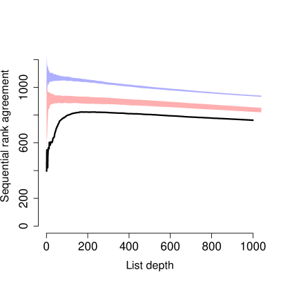
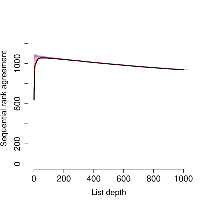
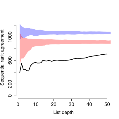
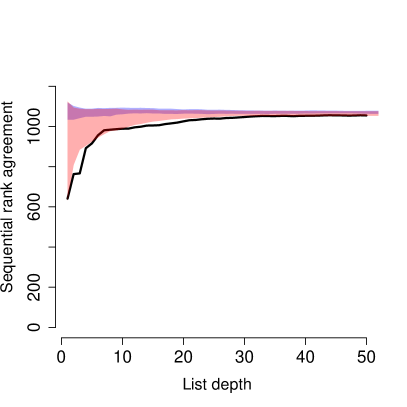
Figure 1: Left panels: Sequential rank agreement for 4 different analysis methods applied to the 3051 genes in the Golub data /black line). Right panels: Corresponding sequential rank agreement for the same data but where only the top 20 ranked items are available. The blue and red areas correspond to the independent and randomized reference hypothesis areas, respectively. The bottom plots are identical to the corresponding top plots but have been zoomed in on the first part of the $x$ axis.

If the lists agree on all items then the sequential rank agreement is zero for all depths. Generally, if there are changes in the level of rank agreement then this suggests that there are sets of items that are ranked similarly in all lists and other sets of items that have been assigned vastly different ranks in the lists. In gene association studies we generally expect the agreement among the lists to be better towards the top of the lists and worse towards the end of the lists. In this case the sequential rank agreement curve will start at a low level and then increase until it levels off as in Figure 1.

2.2 Analysis of partial/censored lists

Incomplete or partial lists are also a common occurrence. They arise for example in case of missing data (items), when comparing top $d$ list results from publications, or when some methods only rank a subset of the items. For example, penalized regression based on the Lasso provides a sparse set of predictors that have non-zero coefficients. There is no obvious ordering of the set of predictors whose coefficient has been shrunk to zero and thus we end up with a partial ordering. Incomplete lists also occur when the analyst decides to censor all lists at depth $d$ such that the measurement of agreement is restricted to the first $d$ elements of each list, or when the analyst only wants to consider the ranking of items that have been found to be statistically significant.

Sequential rank agreement can be generalized to partial lists in the following way. Let $\Lambda_{l}\subset X$ be the subset of $d_{l}$ items that have been ranked highest in list $l$. The case where all lists are censored at the same depth $d$ corresponds to $d_{1}=\cdots=d_{L}=d$. For incomplete/censored lists the rank function becomes

$$\widetilde{R}_{l}(X_{p})=\left\{\begin{array}[]{cl}\{R_{l}(X_{p})\}&\text{ for }X_{p}\in\Lambda_{l}\\ \{d_{l}+1,\dots,P\}&\text{ for }X_{p}\not\in\Lambda_{l}\end{array}\right.$$ (4)

where we only know that the rank for the unobserved items in list $l$ must be larger than the largest rank observed in that list.

The agreement, $A(X_{p})$, cannot be computed directly for all predictors in the presence of censored lists because the exact rank for some items will be unknown. Also, recall that the rankings within a single list are not independent since each rank must appear exactly once in each list. Thus, we cannot simply assign the same number (e.g., the mean of the unassigned ranks) to the censored items since that would result in less variation of the ranks and hence less variation of the agreement, and it would artificially introduce a (downward) bias of agreement for items that are censored in multiple lists.

Instead we randomize the ranks $\{d_{l}+1,\dots,P\}$ to the items that do not occur in list $\Lambda_{l}$. One realization of the $L$ rankings of the set $X$ is obtained by randomizing the missing items of each list. By randomizing a large number of times we can compute (3) for each realization, and then compute the sequential rank agreement as the pointwise (for each depth) average of the rank agreements. The algorithm is described in detail in Algorithm 1.

Algorithm 1 Sequential rank agreement algorithm for censored lists

1:procedure Censored rank agreement

2:     Let $B$ be the number of permutations to use

3:     for each $b\in B$ do

4:         for each censored list $l\in L$ do

5:               Permute the unassigned ranks, $\{d_{l}+1,\ldots,P\}$, and assign them randomly to the items not found in the list, i.e., $\Lambda^{\complement}=X\setminus\Lambda_{l}$. Combine the result with $\Lambda_{l}$ to fill out the list.

6:         end for

7:          Let sra($b$) be the sequential rank agreement computed from the filled out lists.

8:     end for

9:     Return element-wise averages across all $B$ permutations of sra($b$).

10:end procedure

The proposed approach is based on two assumptions: 1) that the most interesting items are found in the top of the lists, and 2) that the censored rankings provide so little information that it is reasonable to assume that they can be represented by a random order. The first assumption is justifiable because we have already accepted that it is reasonable to rank the items in the first place. The second assumption is fair in the light of the first assumption provided that we have a “sufficiently large” part of the top of the lists available.

When the two assumptions are satisfied then it is clear that the interesting part of the sequential rank agreement curves is restricted to the depths where the number of censored items is low. Generally, without additional prior knowledge about the distribution of the censored items it seems reasonable to restrict the attention of the sequential rank agreement to depths smaller than $\max(d_{1},\ldots,d_{L})$ where at least one list provides an uncensored item.

Like for fully observed lists we generally expect the sequential rank agreement to start low and then increase unless the lists are completely unrelated (in which case the sequential rank agreement will be constant at a high level) or if the lists mostly agree on the ranking (in which case the sequential rank agreement will also be constant but at a low level). For partially ranked lists we also expect a change-point around the depth where the lists are censored. This is an artefact stemming from the fact that we assume that the remainder of the lists can be replaced by a simple permutation of the missing items.

3 Evaluating sequential rank agreement

To interpret the sequential rank agreement values we propose two different benchmark values corresponding to two different hypotheses. We wish to determine if we observe better agreement than what would be expected if there were no relevant information available in the data.

The first reference hypothesis is

$$H_{0} :$$ The list rankings correspond to complete randomly

$$\text{permuted lists},$$

which not only assumes that there is no information in the data on which the rankings are based but also that the methods are completely independent.

Alternatively, we can remove the restriction on the independence among the methods by only requiring that there is no information in the ranking but that the rankings are all based on applying the method/approaches to the same data

$$\widetilde{H}_{0} :$$ The list rankings are based on data containing

no association to the outcome.

$H_{0}$ is a quite unrealistic null hypothesis but we can easily obtain realizations from that null hypothesis simply by permuting the items within each list and then computing the sequential rank agreement for the permuted lists. In the fully observed case each experiment contains $L$ lists of random permutations of the items in $X$. For the censored/partially observed case we first permute the items $X_{1},\dots,X_{P}$ and then censor list $l$ at $d_{l}$. The sequential rank agreement curve from the the original lists can then be compared to, say, the pointwise 95% quantiles of the observed rank agreements obtained under $H_{0}$.

To obtain the distribution under $\widetilde{H}_{0}$ the idea is to repeat the ranking procedures for unassociated data many times. Thus, we first permute the outcome variable of the data set on which the rankings are based. This removes any association between the predictor variables and the outcome. Then we apply the methods to the permuted data set to generate $L$ new rankings and subsequently compute the sequential rank agreement. Note that we only permute the outcomes and preserve the structure of the candidate predictors. The randomization approach requires that we have the original data available and as such it may not be possible to evaluate $\widetilde{H}_{0}$ in all situations.

If the sequential rank agreement for the original data lies substantially below the distribution of the sequential rank agreements obtained under either $H_{0}$ or $\widetilde{H}_{0}$ then this suggests that the original ranked lists agree more than what we would expect in data with no information, and therefore that the information in the lists is significantly more in agreement than what would be expected.

Figure 1 shows the empirical distributions of sequential rank agreement under $H_{0}$ and $\widetilde{H}_{0}$ each based on $400$ permutations of the Golub data described in Section 2.1. Not surprisingly, the sequential rank agreement under $\widetilde{H}_{0}$ is lower than the sequential rank agreement under $H_{0}$ because the four methods used to rank the data ($t$ test, logistic regression, elastic net, and MIC) generally tend to identify (and rank) similar predictors even if there are only spurious associations. The two bottom panels in Figure 1 also indicate that the observed sequential rank agreement (the black line) is better than what would be expected by chance for data that contain no information since it lies below the reference areas. However, the censored data also suggests that there may be at most 1 or 2 ranked items towards the top of the lists that yield a result better than what would be expected (the bottom-right plot).

It is important to stress that neither $H_{0}$ nor $\widetilde{H}_{0}$ are related to questions regarding the association between the outcome and the predictors in the data set. Both hypotheses are purely considering how the rankings agree in a situation where there is no relevant information available in the data used for creating the rankings.

4 Comparison to average overlap

The average overlap is a measure that is widely used in comparisons of two fully observed ranked lists (Fagin et al., 2003; Webber et al., 2010) and the idea behind the average overlap closely resembles the sequential rank agreement. In this section we present an extension of the average overlap to more that two lists and compare this to sequential rank agreement.

The overlap among $L$ lists observed until depth $d$ is defined as the proportion of items that are found in all $L$ lists compared to the possible number of items found in all lists observed until depth $d$:

$$O(d)=\frac{|\cap_{l=1}^{L}\{R_{l}^{-1}(r);r\leq d\}|}{d}.$$ (5)

Typically the overlap is only considered for pairwise comparisons (Bar-Ilan et al., 2006; Boulesteix and Slawski, 2009) but formula (5) is easily extended to the situation where $L>2$ as shown above.

The average overlap at depth $d$ is defined as the average of the overlaps until depth $d$,

$$AO(d)=\frac{1}{d}\sum_{i=1}^{d}O(d).$$ (6)

This definition directly ensures that further emphasis is put on items in the top of the lists since their item specific overlap contributes to the calculation of average overlap at higher depths.

There are three main drawbacks of the average overlap method: First it is highly sensitive to single items in the top of one the lists. The average overlap profile may change dramatically depending on the presence or absence of similar items in the beginning of the lists. For example, if all lists have the same item at the top then the average overlap attains its maximum at 1, but if just one of the lists differ then the overage overlap starts at its minimum of 0. Secondly, when the number of lists, $L$, is high then it might be difficult to obtain a non-zero overlap (and hence a non-zero average overlap) at the beginning of the lists because the overlap will be zero until an item is present in all $L$ lists. Finally, the average overlap has an interpretation in terms of moving averages of percentages (of $L$ sets) which is somewhat less intuitive than our proposed sequential rank distance.

In the following we compare the average overlap and the sequential rank agreement using the analysis of the Golub data (Golub, 1999). We consider a typical application of the average overlap and thus restrict attention to only two gene rankings obtained by the $t$ tests and logistic regression. These two marginal modeling approaches should result in very similar gene rankings. The first two columns of Table 2 show the actual top-10 ranking of the predictors.

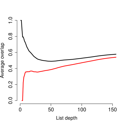
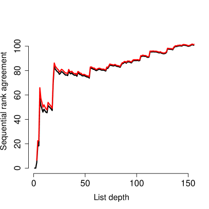
Figure 2: Average overlap (left figure) and sequential rank agreement (right figure) for comparing two different analysis methods (marginal $t$ test and logistic regression) applied to the Golub data. The black lines are based on the full set of predictors while the red lines have the two highest associated predictors removed from the data before computing the average overlap and sequential rank agreement.

The black lines in Figure 2 show the average overlap and sequential rank agreement for these data. It is clear from both plots that there is perfect agreement towards the top of the ranked lists: the average overlap is 1 and the sequential rank agreement is zero. However, if we remove those two items from the data (i.e., gene/predictor 2124 and 896) and redo the analyses then we get substantially different curves for the average overlap but not for sequential rank agreement (red lines in Figure 2). For the sequential rank agreement we get roughly the same estimate of agreement from rank 3 as we did from the full dataset. This indicates that sequential rank is more robust against small perturbations of the data. For the average overlap the curves completely change when these two items are removed and which would lead to a different conclusion about the agreement among the items from rank 3 downwards.

5 Application to ovarian cancer data

We now consider an application of the sequential rank agreement to two data sets consisting of MALDI-TOF (Matrix-Assisted Laser Desorption/Ionization Time Of Flight) mass spectra obtained from blood samples from patients with either benign or malignant ovarian tumors. The data sets are sub-samples of the Danish MALOVA and DACOVA study populations.

The MALOVA study is a multidisciplinary Danish study on ovarian cancer (Hogdall et al., 2004) where all Danish women diagnosed with an ovarian tumor and referred for surgery from the participating departments of gynecology were enrolled continuously from December 1994 to May 1999. For the purpose of illustration we use a random sub-sample of $119$ patients with a total of $58$ patients with malignant ovarian cancers as cases and $61$ patients with benign ovarian tumors as controls. The DACOVA study is another multidisciplinary Danish study on ovarian cancer which included about $66\%$ of the female population of Denmark (Bertelsen, 1991). The study aimed to continuously enroll all patients that were referred to surgery of an ovarian tumor clinically suspected to be cancer during the period from 1984 to 1990. Similarly, we use a random sub-sample from the DACOVA study of $113$ patients with a total of $54$ malignant ovarian cancers and $59$ benign ovarian tumors/gynecologic disorders.

Each spectrum consists of $49642$ samples over a range of mass-to-charge ratios between $800$ to $20000$ Dalton which we downsample on an equidistant grid of 5000 points by linear interpolation. We then preprocess the downsampled spectra individually by first removing the slow-varying baseline intensity with the SNIP algorithm (Ryan et al., 1988) followed by a normalization with respect to the total ion count. Finally, we standardize the $5000$ predictors to have column-wise zero mean and unit variance in each data set.

We use the two data sets to illustrate how the sequential rank agreement can be applied in two different scenarios. In the first scenario we assess the agreement of four different statistical classification methods in how they rank the predictors according to their importance for distinguishing benign and malignant tumors. In the second scenario we assess the agreement among rankings of individual predicted risks of having a malignant tumor. The first scenario is relevant in the context of biomarker discovery and the latter is important e.g., when ranking patients according to immediacy of treatment.

Four classification methods are considered: Random Forest (Breiman, 2001) implemented in the R package randomForest (Liaw and Wiener, 2002), logistic Lasso (Tibshirani, 1996) and Ridge regression (Segerstedt, 1992) both implemented in the R package glmnet (Friedman et al., 2010), and Partial Least Squares Discriminant Analysis (PLS-DA) (Boulesteix, 2004) implemented in the R package caret (Kuhn, 2014).

In both scenarios we use the MALOVA data to train the statistical models, and in both situations the agreements are assessed with respect to perturbations of the training data in the following manner. We repeatedly draw a random sub-sample (without replication) consisting of 90% of the MALOVA observations and train the four models on each sub-sample. We use 1000 iterations for the sub-sampling procedure.

All four methods depend on a tuning parameter. The tuning parameter for Lasso and Ridge regression is the degree of penalization, and for PLS-DA it is the number of components (the dimensionality of the subspace). We estimate these separately for each sub-sample by a 20 times repeated 5-fold cross-validation procedure. For the Random Forest we grow a fixed number of $5000$ trees and let the tuning parameter be the number of predictors randomly sampled at each split. We estimate this by a binary search with respect to minimizing the Out-of-Bag classification error estimate.

The implementation of Lasso and Ridge regression in the glmnet package offers three different cross-validated optimization criteria for the penalty parameter: total deviance, classification accuracy and area under ROC. We apply all three criteria to our data to investigate their effect on the agreements. Note also that the Lasso models produce censored lists depending on the value of the penalty parameter.

5.1 Agreement of predictor rankings

For each of the four methods, each of the 1000 models trained on the 1000 sub-samples of the MALOVA data produces a ranking of the 5000 predictors according to their importance for discriminating between the tumor types. For the Random Forest classifier the predictors are ranked according to the Gini index, while for the logistic Lasso and Ridge regression models we order by absolute magnitude of the estimated regression coefficients. For the PLS-DA model the importance of the predictors is based on a weighted sum of the absolute coefficients where the weights are proportional to the reduction in the sums of squares across the components.

The right panel of Figure 3 shows the sequential rank agreement of the estimated importance of the 5000 predictors. For clarity of presentation we zoom in on the agreement up to list depth 600. At deeper list depths all agreement curves are approximately constant.

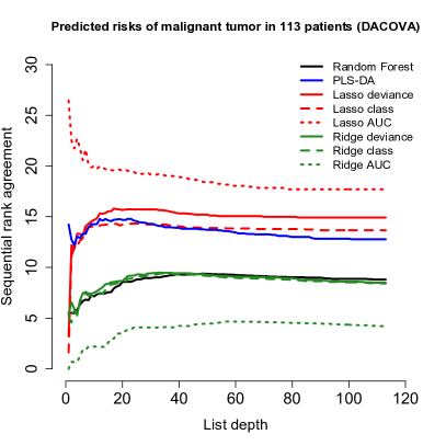
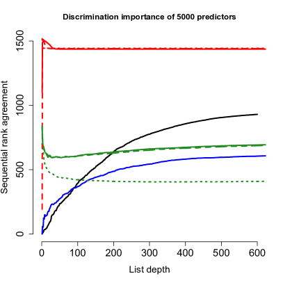
Figure 3: Left panel: Sequential rank agreement of 1000 rankings of the predicted risks of malignant tumor. For each method the different rankings were obtained by first training models in 1000 random sub-samples of the MALOVA data and then predicting the risk of malignant tumor in the 113 DACOVA patients. Right panel: Sequential rank agreement of 1000 rankings of the 5000 predictors. The rankings were obtained from the same 1000 trained models.

For most of the sequential rank agreement curves we see, as expected, that they start low, indicating good agreement, followed by an increase until they approximately become constant. This has the interpretation that the agreement across the different sub-samples is higher in the top as compared to the tail of the lists for all these classification methods. The change-points where the curves become approximately constant are the list depths where the ranks of the remaining items become close to uniformly random.

A not expected shape of the agreement curves is seen for the Ridge models for all three tuning criteria. They all show higher disagreement in the top of the lists followed by a decrease. The reason behind this behavior is rather subtle. Looking at the distribution of the absolute value of the regression coefficients we see that a large proportion of them are numerically very close to zero and have almost equal absolute value. This is a general feature of the Ridge models in this data set and seen for all the 1000 trained models. This implies that when predictors are ranked according to the magnitude of their coefficients, their actual order becomes more uncertain and more close to a random permutation. This problem can be alleviated by truncating all predictors with absolute coefficient values below a given threshold thereby introducing an artificial censoring of the lists. For the Ridge models tuned with the deviance criterion, Figure 4 (left) shows the the sequential rank agreement where for each of the 1000 trained models the predictors were artificially censored when their absolute coefficient value was lower than the $0.1\%$ quantile of the 5000 absolute coefficient values. The curve was calculated using Algorithm 1 with $B=1000$ and $P=5000$. The corresponding curve from Figure 3 (right panel) is shown for comparison. Even though the number of censored predictors is very small compared to the total number of predictors, the effect on the sequential rank agreement is substantial and with the artificial censoring the shape of the curves is as expected, starting low and then increasing.

Looking at the agreement curves for the Lasso models in Figure 3 (right) we clearly see the effect of the sparsity inducing penalization giving rise to censored lists. These curves were similarly calculated using 1 and $1000$ random permutations. Under the deviance optimization criterion the median number of non-zero coefficients was 33 (range 16 to 50) and for the class accuracy criterion 14 (range 4 to 56). These values correspond to the list depths where the agreement curves become constant as a result of the subsequent censoring.

5.2 Agreement of individual risk predictions

To assess the stability of the individual risk predictions we apply the predictors from the DACOVA data set to each of the models. The predicted probabilities are then ranked in decreasing order such that the patients with the highest risk of a malignant tumor appears in the top of the list. Figure 3 (left) shows the sequential rank agreement separately for each method, based on the 1000 risk predictions obtained from the models trained in the same $1000$ random sub-samples of the MALOVA data.

Most curves start low and then increase indicating higher agreement among high risk patients. This is expected if we rank the individuals according to highest risk of disease. However, it is also expected that individuals with very low risk also show high agreement. In this case we order the patients according to (high) risk prediction but we could essentially also have reversed the order to identify the patients that have low risk prediction.

An exception is the risk prediction agreement for the Lasso tuned with the AUC criterion which shows very low agreement among the high values of the predicted risks. The reason is that optimizing the penalty parameter with respect to the AUC criterion tends to favor a very high penalty value causing only a single predictor to be selected in each of the 1000 iterations. This results in a lack of generalizability to the DACOVA data which gives rise to the higher disagreement in the predicted risks. In the extreme case where the penalty becomes so high that none of the predictors are selected by the Lasso, the sequential rank agreement for the predicted probabilities becomes undefined since all the ranks will be ties.

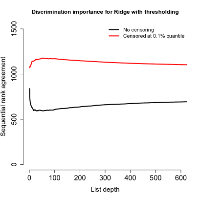
Figure 4: Left panel: Sequential rank agreement for Ridge regression obtained by artificially censoring predictors when their absolute coefficient values are lower than the 0.1% quantile. Right panel: Box plots of AUC values across the $1000$ sub-samples with respect to the known class labels of the DACOVA data.

Comparing the left and right panels of Figure 3 it can further be seen that some of the methods show better agreement with respect to the predicted probabilities than for ranking the importance of the predictors and vice versa. Ridge regression shows higher agreement across training sets for the risk predictions than PLS-DA, and PLS-DA shows higher agreement for predictor importance than Ridge regression.

Lasso shows similar agreement for ranking the risk predictions than PLS-DA (unless with the AUC criterion), and poorer agreement for ranking predictors. This reason for the latter is the high auto-correlation between the intensities in the mass spectra which leads to collinearity issues in the regression models. It is well-known that variable selection with the Lasso penalty does not preform very well when the predictors are highly correlated. The collinearity does, however, not affect the agreement of the risk predictions, as seen on the left panel of Figure 3, since it is not so important which specific variable that gets selected from a group of highly correlated predictors when the purpose is risk predictions.

It appears that Ridge regression tuned with the AUC criterion achieves the best performance with respect to the stability of ranking the individual predicted risk probabilities. It must, however, be stressed that the sequential rank agreement in this application is only concerned with the agreement of the risk predictions across sub-samples and not with the actual accuracy of the risk predictions. Thus, we also computed the AUC values for the different models based on the DACOVA data. The distributions across the $1000$ sub-samples for a selection of the models is shown in the right panel of Figure 4. Here we see that PLS-DA attains the highest AUC values with a median value of $0.70$ while the Ridge model with the AUC criterion attains a median AUC of $0.49$. This implies that while Ridge regression optimized with respect to the AUC criterion achieves the best sequential rank agreement, it performs similar to a random coin toss with respect to classifying the DACOVA patients. In practice both concerns are of importance.

6 Discussion

In this article we address the problem of comparing ranked lists of the same items. Our proposed method can handle both the situation where the underlying data to generate the ranked lists are available and the situation where the only available data is the actual ranked lists. In addition, censored ranked lists where only the ranks of the top $k$ ranked items are known can be accommodated as well. The proposed agreement measure can be interpreted as the average distance between an item’s rank and the average rank assigned to that item across lists. Thus the measure determines how well the lists agree on the ranks of a specific item.

The sequential rank agreement is extremely versatile. We have shown that it can be used not only to compare ranked lists of items produced from different samples/populations but that it also can be used to study the ranks obtained from different analysis methods on the same data as well as to evaluate the stability of the ranks from a single method by bootstrapping (or sub-sampling) the data repeatedly and comparing the ranks obtained from training the models in the bootstrapped data.

The sequential rank agreement can be used to determine the depth at which the rank agreement becomes too large to be desirable based on prior requirements or acceptable differences, or it can be used to visually determine when the change in agreement becomes too large. In that regard the investigator can have prior limits on the level of agreement that is acceptable.

While the sequential rank agreement is primarily an exploratory tool we have suggested two null hypotheses that can be used to evaluate the sequential rank agreement obtained. Note that none of the two null hypotheses are concerned with the actual “true ranking” but are purely concerned with consistency/stability of the rankings among the lists. As such we cannot determine if the rankings are good but only whether they agree. The sequential rank agreement curve can be compared visually to the curves obtained under either of the null distributions and simple point-wise $p$-values can be obtained for each depth by counting the number of sequential rank agreements under the null hypothesis that is less than or equal to the observed rank agreement. Two simple extensions can be pursued to make more formal uniform tests: one would be to use a Kolmogorov-Smirnov-like test and use the largest difference between the variance-weighted sequential rank agreement curve and the mean null rank agreement curve as a test statistic. Alternatively, a change-point analysis could be made on the sequential rank agreement in order to determine the depths at which there are “jumps” in the rank agreement. These jumps would correspond to depths for which the agreement among the lists was substantially worse and could serve as indicators for when the lists no longer agree sufficiently satisfactory.

Finally, we have — whenever possible — used all available ranks from the lists. We could choose to censor the rankings of all the items that were deemed not to be significant if information on both rankings and the corresponding evidence for significance was available. That would ensure that there would be put less emphasis on the agreement of the non-significant items and it would be easier to identify a change in agreement among the items that were deemed to be relevant. In our application section we have successfully introduced such an artificial censoring for the predictor rankings obtained with ridge regression.

We note that the sequential rank agreement is still marred by problems that generally apply to ranking of items and/or individuals. Collinearity in particular can be a huge problem when bootstrapping data or when comparing different analysis methods. For example, marginal analyses where each item is analyzed separately will assign similar ranks to two highly correlated predictors while methods that provide a sparse solution such as the Lasso will just rank one of the two predictors high while the other might have a very low rank. Thus in such a scenario we would expect low agreement of the rankings from Lasso and marginal analyses simply because of the way correlated predictors are handled. This is not a shortcoming of the sequential rank agreement but is a problem general to all ranked lists.

Another caveat with the way the sequential rank agreement is defined is the use of the standard deviation to measure agreement. The standard deviation is an integral part of the limits-of-agreement as discussed by Altman and Bland (1983). However, the standard deviation can also be unstable when the number of observations is low and alternative measures such as the median absolute deviance may prove more stable in some situations. However, the current definition using the standard deviation is analogous to the approach used for agreement in method comparison studies so we have used that.

In conclusion we have introduced a method for evaluation of ranked (censored) lists that can be easily interpreted and that can be applied to a large number of situations. The method presented here can be adapted further by using it to compare and classify statistical analysis methods that agree on the rankings they provide or by using the rank agreement to optimize a hyper-parameter in, say, elastic net regularized regression where the rank agreement is used to determine the mixing proportion between the $L_{1}$ and the $L_{2}$ penalty. We will be investigating these extensions further in the future.

References

- Altman and Bland (1983) Altman, D. and Bland, J. M. (1983) Measurement in medicine: the analysis of method comparison studies. The Statistician, 32, 307–317.
- Bar-Ilan et al. (2006) Bar-Ilan, J., Mat-Hassan, M. and Levene, M. (2006) Methods for comparing rankings of search engine results. Computer Networks, 50, 1448–1463.
- Bertelsen (1991) Bertelsen, K. (1991) Protocol allocation and exclusion in two Danish randomised trials in ovarian cancer. British journal of cancer, 64, 1172.
- Boulesteix (2004) Boulesteix, A.-L. (2004) PLS dimension reduction for classification with microarray data. Statistical applications in genetics and molecular biology, 3, 1–30.
- Boulesteix and Slawski (2009) Boulesteix, A.-L. and Slawski, M. (2009) Stability and aggregation of ranked gene lists. Briefings in Bioinformatics, 10, 556–568.
- Breiman (2001) Breiman, L. (2001) Random forests. Machine learning, 45, 5–32.
- Carstensen (2010) Carstensen, B. (2010) Comparing Clinical Measurement Methods: A Practical Guide. Wiley.
- Carterette (2009) Carterette, B. (2009) On rank correlation and the distance between rankings. In Proceedings of the 32Nd International ACM SIGIR Conference on Research and Development in Information Retrieval, SIGIR ’09, 436–443. New York, NY, USA: ACM.
- Dudoit et al. (2002) Dudoit, S., Fridlyand, J. and Speed, T. P. (2002) Comparison of Discrimination Methods for the Classification of Tumors Using Gene Expression Data. Journal of the American Statistical Association, 97, 77–87.
- Fagin et al. (2003) Fagin, R., Kumar, R. and Sivakumar, D. (2003) Comparing Top k Lists. SIAM Journal on Discrete Mathematics, 17, 134–160.
- Friedman et al. (2010) Friedman, J., Hastie, T. and Tibshirani, R. (2010) Regularization paths for generalized linear models via coordinate descent. Journal of statistical software, 33, 1–22.
- Golub (1999) Golub, T. R. (1999) Molecular Classification of Cancer: Class Discovery and Class Prediction by Gene Expression Monitoring. Science, 286, 531–537.
- Hogdall et al. (2004) Hogdall, E. V., Ryan, A., Kjaer, S. K., Blaakaer, J., Christensen, L., Bock, J. E., Glud, E., Jacobs, I. J. and Hogdall, C. K. (2004) Loss of heterozygosity on the X chromosome is an independent prognostic factor in ovarian carcinoma: from the Danish ”MALOVA” ovarian carcinoma study. Cancer, 100, 2387–2395.
- Kendall (1948) Kendall, M. G. (1948) Rank Correlation Methods. Griffin.
- Kuhn (2014) Kuhn, M. (2014) caret: Classification and Regression Training. R package version 6.0-24.
- Liaw and Wiener (2002) Liaw, A. and Wiener, M. (2002) Classification and regression by randomForest. R news, 2, 18–22.
- Reshef et al. (2011) Reshef, D. N., Reshef, Y. A., Finucane, H. K., Grossman, S. R., McVean, G., Turnbaugh, P. J., Lander, E. S., Mitzenmacher, M. and Sabeti, P. C. (2011) Detecting novel associations in large data sets. Science (New York, N.Y.), 334, 1518–24.
- Ryan et al. (1988) Ryan, C. G., Clayton, E., Griffin, W. L., Sie, S. H. and Cousens, D. R. (1988) SNIP, a statistics-sensitive background treatment for the quantitative analysis of PIXE spectra in geoscience applications. Nuclear Instruments and Methods in Physics Research Section B: Beam Interactions with Materials and Atoms, 34, 396–402.
- Segerstedt (1992) Segerstedt, B. (1992) On ordinary ridge regression in generalized linear models. Communications in Statistics-Theory and Methods, 21, 2227–2246.
- Shieh (1998) Shieh, G. S. (1998) A weighted Kendall’s tau statistic. Statistics & Probability Letters, 39, 17–24.
- Spearman (1910) Spearman, C. (1910) Correlation calculated from faulty data. British Journal of Psychology, 3, 271–295.
- Tibshirani (1996) Tibshirani, R. (1996) Regression shrinkage and selection via the lasso. Journal of the Royal Statistical Society. Series B (Methodological), 267–288.
- Webber et al. (2010) Webber, W., Moffat, A. and Zobel, J. (2010) A similarity measure for indefinite rankings. ACM Trans. Inf. Syst., 28, 20:1–20:38.
- Yilmaz et al. (2008) Yilmaz, E., Aslam, J. A. and Robertson, S. (2008) A new rank correlation coefficient for information retrieval. In Proceedings of the 31st Annual International ACM SIGIR Conference on Research and Development in Information Retrieval, SIGIR ’08, 587–594. New York, NY, USA: ACM.