Abstract

The robust estimation of dynamically changing features, such as the position of prey, is one of the hallmarks of perception. On an abstract, algorithmic level, nonlinear Bayesian filtering, i.e. the estimation of temporally changing signals based on the history of observations, provides a mathematical framework for dynamic perception in real time. Since the general, nonlinear filtering problem is analytically intractable, particle filters are considered among the most powerful approaches to approximating the solution numerically. Yet, these algorithms prevalently rely on importance weights, and thus it remains an unresolved question how the brain could implement such an inference strategy with a neuronal population. Here, we propose the Neural Particle Filter (NPF), a weight-less particle filter that can be interpreted as the neuronal dynamics of a recurrently connected neural network that receives feed-forward input from sensory neurons and represents the posterior probability distribution in terms of samples. Specifically, this algorithm bridges the gap between the computational task of online state estimation and an implementation that allows networks of neurons in the brain to perform nonlinear Bayesian filtering. The model captures not only the properties of temporal and multisensory integration according to Bayesian statistics, but also allows online learning with a maximum likelihood approach. With an example from multisensory integration, we demonstrate that the numerical performance of the model is adequate to account for both filtering and identification problems. Due to the weightless approach, our algorithm alleviates the ’curse of dimensionality’ and thus outperforms conventional, weighted particle filters in higher dimensions for a limited number of particles.

Author Summary

Every day, our brain is facing the challenge of making sense of the rich and dynamical stream of sensory inputs. Those inputs are often ambiguous, noisy and sometimes even conflicting. That we are nevertheless able to make sense of our surrounding naturally points to the important question how estimates of real-world variables that led to perceptive input, e.g. the position or the velocity of an object, are formed. Further, it is unknown how the computational task of real-time state estimation can be implemented in a realistic neuronal architecture. Here, we propose an algorithm, the Neural Particle Filter, that performs state estimation, in a way that captures essential properties of perception: it takes into account prior knowledge of the environment, weights different sensory modalities according to their reliability and is able to dynamically adapt to changes. Implemented as a neuronal dynamics, the Neural Particle Filter predicts activation properties of the neurons involved in perception.

Introduction

During the last decade, an increasing number of studies have stated that the brain performs probabilistic inference during perceptual tasks [1, 2]. As an act of (approximate) Bayesian inference, perception relies on noisy and incomplete data that needs to be integrated across multiple sensory modalities and weighted according to sensory reliability. In addition, perception makes use of the strong statistical regularities of objects in our environment by forming prior beliefs about the world. Since our environment is fundamentally dynamic, the ability to adapt to changes in real time is essential for perception. The Bayesian brain hypothesis is supported by ample experimental evidence, ranging from psychophysical findings [3, 4, 5] to neuronal recordings [6, 7, 8] that are in line with Bayesian computation. However, most of the studies concerned with the theory of perception consider fairly simple tasks, where the observations are created either from static hidden variables [9] or from hidden variables with a discrete state-space [10], or the underlying dynamics are considered linear [11, 12].

In a dynamical setting, where temporally changing signals have to be estimated online from the history of observations, Bayesian inference is commonly referred to as ‘filtering’. In general, nonlinear Bayesian filtering is a challenging task even without the imperative of a plausible implementation on a neuronal architecture. If the prior distribution is a Gaussian and the noisy observations depend linearly on the hidden states, the inference problem is solved by the Kalman filter [13, 14], which has received substantial attention in the signal processing community and turns out to be of increasing importance in neuroscientific phenomenological modeling, e.g. in a sensorimotor integration task [3] or in estimating motor disturbances from an adaptive gain [15]. Solutions for the more general nonlinear, i.e. non-Gaussian, filtering problem [16, 17] are analytically intractable and thus have to be approximated.

Sampling-based approaches have proven to be a powerful tool to solve the nonlinear filtering problem numerically. In principle, they enable any posterior distribution to be represented with an accuracy that depends on the number of samples. On the one hand, so called particle methods (see for instance [18, 19]) are well suited for dynamical priors, but suffer in high dimensions due to the degeneracy of the importance weights and it is still unclear how to implement such an inference scheme in a neuronal network. On the other hand, Langevin sampling [20, 21] and related techniques, such as the ‘fast sampler’ in [22], provide a promising ground for a biologically plausible implementation of neural or synaptic sampling [23, 24], but are restricted to static generative models.

Following a sampling-based approach, we propose a framework for how the brain could perform filtering from noisy sensory stimuli, considering Marr’s three levels [25]: the computational level, the algorithmic and representational level and the implementation level. On the first level, the computational task of dynamical state estimation is set in the context of continuous-time continuous-state nonlinear filtering theory. Motivated by this rigorous mathematical theory, we propose a weight-less particle filter, the Neural Particle Filter (NPF), that approximates the posterior at each time step by sampling from it. This algorithm can further be tuned by maximum likelihood learning and thus allows for rigorous corrections in the algorithmic ansatz, as well as learning the model parameters. The NPF exhibits properties that are considered crucial for perception. On the implementation level, we interpret the NPF as a biologically plausible neuronal dynamics and identify the particle states with activities of task-specific neurons.

Results

The results we are presenting are subdivided in two parts: first, we will introduce the Neural Particle Filter as a conceptual result. This first part will cover the first two of Marr’s three levels, namely i.) the computational level with a generative model layout and a task description, and ii.) the algorithmic level, which outlines our choice of representation and the approximate solution to the nonlinear filtering problem that is based on this representation. In the second part, we demonstrate key properties of the NPF, and we we illustrate how they might serve as a model for a neuronal dynamics involved in perception.

Model

Nonlinear filtering as a generic computational task

We formulate the computational task in terms of the classical filtering problem (according to standard literature on nonlinear filtering, e.g. [26, 27]). The hidden state $\mathbf{x}_{t}\in\mathbb{R}^{n}$, i.e. the real-world variable that the brain cannot access directly, follows the Itô stochastic differential equation (SDE):

$$d\mathbf{x}_{t} = \mathbf{f}(\mathbf{x}_{t})\,dt+\Sigma_{x}^{1/2}\,d\boldsymbol{\omega}_{t},$$ (1)

with a nonlinear, deterministic drift function $\mathbf{f}(\mathbf{x}):\mathbb{R}^{n}\to\mathbb{R}^{n}$. Stochastic diffusion is governed by the uncorrelated Brownian motion process $\boldsymbol{\omega}_{t}\in\mathbb{R}^{n}$ with noise covariance $\Sigma_{x}\in\mathbb{R}^{n}\times\mathbb{R}^{n}$.

At each moment in time, the hidden state $\mathbf{x}_{t}$ gives rise to noisy observations $\mathbf{y}_{s}\in\mathbb{R}^{m}$ that represent sensory input. The observation dynamics is again modeled in terms of an Itô diffusion, with a drift term following the hidden states via a generative function $\mathbf{g}(\mathbf{x}):\mathbb{R}^{n}\to\mathbb{R}^{m}$ and a Brownian motion diffusion, modulated by the sensory noise covariance $\Sigma_{y}\in\mathbb{R}^{m}\times\mathbb{R}^{m}$:

$$d\mathbf{y}_{t} = \mathbf{g}(\mathbf{x}_{t})\,dt+\Sigma_{y}^{1/2}\,d\boldsymbol{\nu}_{t}.$$ (2)

Together, Eqs. (1) and (2) define a generative model.

Solving the filtering problem is the task of finding the posterior probability $p(\mathbf{x}_{t}|\mathcal{Y}_{t})$ of the hidden state, conditioned on the whole sequence of observations $\mathcal{Y}_{t}=\{\mathbf{y}_{s},s\in[0,t]\}$ up to time $t$. For a linear hidden dynamics $\mathbf{f}(\mathbf{x})$ and a linear observation dynamics $\mathbf{g}(\mathbf{x})$, this task is solved by the Kalman-Bucy filter [14], which is a continuous-time version of the well-known Kalman filter. However, the solution to the nonlinear filtering problem is in general analytically intractable, because it suffers from the so-called closure problem (see S1 Appendix.). Therefore, introducing a suitable approximation is an inevitable step when approaching the nonlinear filtering problem.

Sampling-based representation

We approximate probability distributions in terms of a finite number of variables. For example, this can be achieved by taking $N$ weighted samples:

$$p(\mathbf{x},t) \approx \sum_{k=1}^{N}w_{k}\,\delta(\mathbf{x}-\mathbf{x}_{t}^{(k)}),\ \text{with }\sum_{k=1}^{N}w_{k}=1.$$ (3)

Thus, the probability of the random variable to have a certain value range is proportional to the relative number of samples within this range, weighted by their respective weight $w_{i}$.

Filtering algorithms representing the posterior in this sampling-based manner are commonly referred to as particle filters. In standard particle filters (such as outlined in [28]), update rules for the trajectories $\mathbf{x}_{t}^{(k)}$, as well as the weights $w_{k}$ are given. Despite asymptotic convergence to the true posterior for an infinite number of particles, this approach has two disadvantages: First, one finds numerically that after a finite number of time-steps most particle weights decay to zero, which depletes the number of effective samples. Weight decay, or degeneration, is an undesirable trait of weighted particle methods in general. As stated in the convergence theorem [29, Theorem 23.5], the upper bound of the divergence between true posterior and the posterior estimated by the weighted particle system is a function of time, and hence might be growing due to the weight decay. Second, the problem is exacerbated if the number of dimensions of the hidden state $\mathbf{x}_{t}$ is large. In this case, the number of particles needed for good numerical performance grows exponentially with the number of dimension, a variant of the ‘curse of dimensionality’ [30].

In the theoretical neuroscience literature, sampling-based approaches for filtering with a representation of the posterior as in Eq. (3) have not received much attention so far (one of the few examples can be found in [31]), although they have some experimental support [32, 7] and are considered relevant according to the neural sampling hypothesis [33]. Therefore, we would like to explore this approach further. To overcome the difficulties encountered with weighted approaches, we consider a particle filter with equally weighted samples, i.e. $w_{k}=1/N\ \forall k$.

Filtering with the Neural Particle Filter

As an inference algorithm, we propose an SDE that governs the dynamics of particles $\mathbf{z}_{t}$. Let us consider $N$ i.i.d. stochastic processes $\mathbf{z}_{t}^{(k)},\ k=1,\dots,N$, conditioned on the observations $\mathcal{Y}_{t}$, following the Itô diffusion

$$d\mathbf{z}_{t}^{(k)} = \mathbf{f}(\mathbf{z}_{t}^{(k)})\,dt+W_{t}\big{(}d\mathbf{y}_{t}-\mathbf{g}(\mathbf{z}_{t}^{(k)})\,dt\big{)}+\Sigma_{x}^{1/2}\,d\mathbf{w}_{t},$$ (4)

where $\mathbf{w}_{t}\in\mathbb{R}^{n}$ is an uncorrelated vector Brownian motion process and $W_{t}$ is a time-dependent gain matrix or decoding weight matrix.

Equation (4), which we will further refer to as the Neural Particle Filter (NPF), is an ansatz that serves as a sampling-based approximation to the nonlinear filtering problem: we consider each of the $N$ stochastic processes $\mathbf{z}_{t}^{(k)}$ as an independent sample, or particle, of the true posterior $p(\mathbf{x}_{t}|\mathcal{Y}_{t})$ at every time $t$. Thus, expectations from the posterior are computed according to $\mathbb{E}[\phi(\mathbf{x}_{t})|\mathcal{Y}_{t}]\approx\langle\phi(\mathbf{x}_{t})\rangle=1/N\sum_{k}\phi(\mathbf{z}_{t}^{(k)})$.

This ansatz is motivated by the formal solution to the filtering problem, more precisely by the dynamics of the first posterior moment and shares some important properties with classical filtering methods: First, it is governed by both the dynamics of the hidden process $\mathbf{x}_{t}$ and by a correction proportional to the so-called innovation term $d\mathbf{n}_{t}=d\mathbf{y}_{t}-\mathbf{g}(\mathbf{z}_{t})\,dt$. The innovation term compares the sensory input $d\mathbf{y}_{t}$ with the current prediction $\mathbf{g}(\mathbf{z}_{t})\,dt$ according to the single particle position, and thus can be seen as a predictive error signal [9]. Second, the gain matrix $W_{t}$ determines the emphasis that is laid on new information via observations $d\mathbf{y}_{t}$. This is conceptually similar to a Kalman gain [13, 14] for a linear model, and adjusts according to the reliability of a single or multiple observations.

The gain introduces a weighting between the prior probability distribution $p(\mathbf{x}_{t})$ induced by Eq. (1), and the likelihood function $p(\mathbf{y}_{t}|\mathbf{x}_{t})$ induced by Eq. (2) and thus serves as a measure for the peakedness of the likelihood. If the decoding weight is large, the dynamics in Eq. (4) will entirely be determined by the innovation term, and the inter-particle variability governed by the diffusion term will be negligible. Therefore, the resulting probability distribution is given by $p(\mathbf{x}_{t}|\mathcal{Y}_{t})\approx p(\mathbf{z}_{t}|\mathcal{Y}_{t})\sim\delta(\mathbf{z}_{t}-\mathbf{g}^{-1}(\frac{d\mathbf{y}_{t}}{dt}))$. In this limit, the deterministic observation limit, a single sample from Eq. (4) suffices to represent the posterior. On the other hand, if the decoding weight is zero, new information is disregarded, and each sample evolves just like an i.i.d. process from Eq. (1).4 In this case, the resulting probability distribution simply equals the stationary prior distribution $p(\mathbf{x}_{t})$.

For the gain $W_{t}$, we use the ansatz $W_{t}=\text{cov}(\mathbf{x}_{t},\mathbf{g}(\mathbf{x}_{t})^{T})\Sigma_{y}^{-1}$, an empirical choice motivated by the mean dynamics of the formal solution. This gain adjusts according to the observation noise $\Sigma_{y}$ as well as to the spatial ambiguity as measured by the empirical, i.e. instantaneously estimated from the particle positions, covariance between the state $\mathbf{x}_{t}$ and the observation function $\mathbf{g}(\mathbf{x}_{t})$ (Eq. 13 in Methods). Although this choice is rather heuristic, it achieves a numerical performance comparable to that of a standard particle filter (PF), as demonstrated below, and is moreover straightforward to implement by empirically estimate the covariance from the particle positions.

Parameter learning

In a more general setting, model parameters of Eqs. (1) and (2) may not or only partially be known, and thus need to be learned online from the stream of observations $\mathcal{Y}_{t}$. In this case, the NPF algorithm can be extended to include a parameter update that performs an online gradient ascent on the log likelihood

$$L^{\text{online}}_{t}(\theta)=\langle\mathbf{g}(\mathbf{x}_{t})\rangle^{T}\Sigma_{y}^{-1}\,d\mathbf{y}_{t}-\frac{1}{2}\langle\mathbf{g}(\mathbf{x}_{t})\rangle^{T}\Sigma_{y}^{-1}\langle\mathbf{g}(\mathbf{x}_{t})\rangle\,dt,$$ (5)

which in turn is computed directly from the approximated filtering distribution itself. It can be shown that maximizing this log likelihood is equivalent to minimizing the prediction error in continuous time (see S1 Appendix.).

Further, not only the model parameters in Eqs. (1) and (2), but also the decoding parameters, i.e. components of the decoding weight or gain matrix $W_{t}$, can be learned with a maximum likelihood approach, instead of setting it according to the empirical estimate from the particle positions. This alternative corrects for the heuristic ansatz of the NPF equation (4) by determining the decoding weights rigorously. In fact, it can be shown that parameter learning with a maximum likelihood approach is able to make up even for a very poor filtering ansatz by setting parameters accordingly [35].

The Neural Particle Filter as a neuronal dynamics for perception

In this section, we set the computational task in the context of perception and base the implementation of the algorithm on a neuronal architecture. With a simple example, we now illustrate that our algorithm captures the following key properties of perception [2]: 1) it relies on noisy and incomplete sensory data, 2) it uses prior knowledge of the dynamic structure of the environment 3) it efficiently combines information from several sensory modalities, and 4) it can dynamically adapt to changes in the environment.

Multisensory perception as filtering

Consider a frog who sits below two branches and observes an insect flying between the two branches (Fig. 1a). The frog wants to track the position of the insect $x_{t}$, which is governed by

$$dx_{t} = 3x_{t}\big{(}1-x_{t}^{2}\big{)}\,dt+d\omega_{t},$$ (6)

where the Brownian motion process $\omega_{t}$ accounts for noise due to the erratic behavior of the insect. This dynamics gives rise to a bimodal stationary distribution for the position of the insect (cf. Fig. 1a).

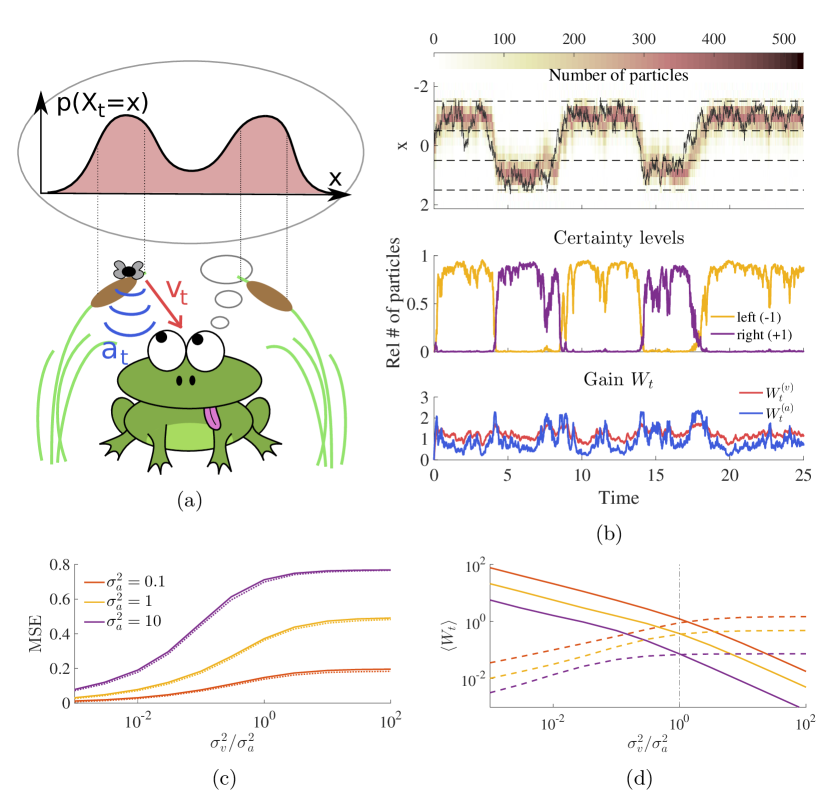
Figure 1: The NPF as a model for perception for multisensory perception. (a) The frog has to do filtering in order to dynamically track the position $x_{t}$ of the insect, which is switching between two branches. We model this behavior by the stochastic dynamics in Eq. (6), which gives rise to a bimodal prior distribution $p(x_{t}=x)$. In order to track the insect, the frog has to make use of this prior, and optimally combine it with the noisy input from the sensory modalities $v_{t}$ and $a_{t}$. (b) Tracking simulation with $N=1000$ filtering neurons and sensory noise $\sigma_{v}^{2}=\sigma_{a}^{2}=0.1$. The upper panel shows the true trajectory of the insect (solid black line) and particle densities. The regions between the dotted black lines denote the two branches, and certainty levels certainty levels in the middle panel correspond to the relative number of particles whose states are within one of the two branches. At each time, the sensory gains in the lower panel are computed according to Eqs. (10) and (11). (c) Performance in terms of time-averaged mean-squared error $MSE=\langle(x_{t}-\hat{x}_{t})^{2}\rangle_{t}$ (dotted lines: standard particle filter) and (d) time-averaged gains $\langle W_{t}^{(v)}\rangle_{t}$ (solid line) and $\langle W_{t}^{(a)}\rangle_{t}$ (dashed line) as function of sensory noise.

The frog cannot directly observe the state $x_{t}$ of the insect, but instead has to rely on two sensory channels, a visual ($v_{t}$) and an auditory ($a_{t}$) channel. Observation dynamics in these channels are given by

$$dv_{t} = x_{t}\,dt+\sigma_{v}d\beta_{t},$$ (7)

$$da_{t} = \text{tanh}(2x_{t})\,dt+\sigma_{a}d\gamma_{t},$$ (8)

where $\beta_{t},\gamma_{t}$ are independent Brownian motions that model noise in the sensory channels, making $v_{t}$ and $a_{t}$ conditionally independent. The nonlinearity in the auditory channel (Eq. 8) is motivated by the fact that sound localization depends on interaural difference, which resembles a sigmoid in this example. In order to localize the fly, the frog has to perform the task of nonlinear filtering and to compute $\hat{x}_{t}=\mathbb{E}[x_{t}|v_{s},a_{s},0\leq s\leq t]$, i.e. the position of the insect, from the visual and auditory sensory streams. Note that due to the nonlinear dynamics of the hidden and observation processes, this example is analytically intractable and thus requires an approximation.

We propose that this task is solved by a set of $N$ filtering neurons $z_{t}^{i}$, $i=1,...,N$. Their neuronal dynamics are given by the NPF (4) and for this particular example read:

$$dz_{t}^{(i)} = 3z_{t}^{(i)}\big{(}1-(z_{t}^{(i)})^{2}\big{)}\,dt+d\omega^{(i)}_{t}$$ (9)

$$+W^{(v)}_{t}\big{(}dv_{t}-z_{t}^{(i)}\,dt\big{)}+W^{(a)}_{t}\big{(}da_{t}-\text{tanh}(2z_{t}^{(i)})\,dt\big{)},$$

which is governed by the dynamics of the prior as well as corrections evoked by novelty of the observations in the sensory channels, that are modulated by gains $W^{(v)}_{t}$ and $W^{(a)}_{t}$. Thus, our model readily captures the first two key properties of perception.

The empirical distribution of neuronal activities $z_{t}^{(i)}$ approximately samples the posterior distribution, thereby acting as a weight-less particle filter that successfully tracks the position of the insect (Fig. 1b). The state estimate $\hat{x}_{t}$ (posterior mean) can be read out from this population by averaging the activities of the filtering neurons, i.e. $\hat{x}_{t}\approx\langle z_{t}\rangle=N^{-1}\sum_{i}z_{t}^{(i)}$.

The potential of having a description of the full posterior stretches far beyond simple state estimation, where one is only interested in the first moment. Particularly the sampling-based approximation of this posterior allows a convenient estimation of other relevant quantities. For example, the frog might want to know on which branch the insect is sitting in order to catch it more easily. The frog could directly deduce a certainty level for the left and right branch, respectively (Fig. 1b), by counting the number of neurons within a certain activity range.

In a similar manner, higher-order moments of the posterior distribution can be approximated with the samples that correspond to neuronal activities. Even though these approximated moments are not exact (Fig. 2c), the overall posterior shape is captured to a considerable extent. For some nonlinearities, our proposed model is therefore superior to models relying on an approximation of just the first two moments of the distribution. For instance, the Extended Kalman Filter (EKF) does by definition not capture higher order moments of the posterior and thus fails to reproduce its features. This explains why the predictive performance of the EKF in terms of MSE is fairly poor compared to that of the NPF (Fig. 2a,b).

Figure 2: MSE and estimation of posterior variance from single-cue observation. Simulations correspond to the example model with only (a) visual or (b) auditory cue, i.e. a generative model with Eqs. (6) and (7) or (8), respectively. The gain in the NPF is tuned according to $W_{t}=\text{cov}(\mathbf{x}_{t},\mathbf{g}(\mathbf{x}_{t})^{T})\Sigma_{y}^{-1}$ and according to a gradient ascent on the log likelihood (‘ML’), respectively For benchmarking, we use a standard PF. The performance of the NPF is nearly indistinguishable to that of the PF. In addition, we compare the performance of an EKF. (c) The posterior variance $\hat{\Sigma}$ on average exhibits a bias $\text{Bias}(\hat{\Sigma})=\hat{\Sigma}-\Sigma_{PF}$ when compared to that of the PF. Here, solid (dashed) lines refer to the visual (auditory) channel.

Cue integration

The decoding weights, or gain factors, $W_{t}^{(v)}$ and $W_{t}^{(a)}$, are exemplary for essential multisensory integration. They balance the relative effects of the two sensory modalities and the prior on the dynamics of the filtering neurons and thus quantify the reliability of the sensory channels. Here, we consider $W_{t}=\text{cov}(\mathbf{x}_{t},\mathbf{g}(\mathbf{x}_{t}))\Sigma_{y}^{-1}$ in the NPF. Thus, in this example, the weights evaluate to

$$W_{t}^{(v)}=\text{Var}(x_{t})\sigma_{v}^{-2}$$ (10)

$$W_{t}^{(a)}=\text{Cov}(x_{t},\text{tanh}(2x_{t}))\sigma_{a}^{-2},$$ (11)

where posterior variances and covariances are estimated empirically from the neuronal activity distribution. The gains adjust according to both the sensory noise levels (Fig. 1d) and the spatial ambiguity evoked by the sigmoid observation function for the auditory channel $a_{t}$ (Fig. 1b). In particular, the gains become large if a channel is particularly reliable, and in extreme cases dominate the dynamics of the filtering neurons, corresponding to the deterministic observation limit discussed earlier. The appropriate weighting of sensory information allows the neurons to solve the filtering task near-optimally and comparable to a standard PF, which is reflected by our simulation results in Fig. 1c and 2a,b.

Adapting to changes

In our example, the frog could successfully track the position of the insect, but it could only do so because it had access to the generative model parameters, i.e. it knew the prior dynamics of the insect and it it was aware of how the sensory percepts were generated from the true state of the insect. Also, knowledge of these model parameters were crucial for determining the sensory weights $W_{t}^{(v)}$ and $W_{t}^{(a)}$ and thus significantly influenced the dynamics of the filtering neurons. However, the external world, i.e. the model parameters, does change over time, and successful perception should adapt accordingly, i.e. the model parameters should be adjusted by online learning from the stream of observations $\mathcal{Y}_{t}$.

We illustrate the learning of generative model parameters using our example (see Methods and S1 Appendix. for details). This time, the frog only relies on his visual channel $v_{t}$, but in addition to tracking the insect, he also has to learn the generative factor $J$ in the function $g(x)=Jx$, which relates the position of the insect to the visual input. Simultaneously, it also learns the gain $W_{t}^{(v)}$ and with that implicitly an estimate of the reliability of its visual input. Figure 3 shows that this identification problem can be solved efficiently by the NPF, with an MSE that gradually approaches that of the benchmark (a standard PF with the ground-truth parameters) as the estimate of the parameters get more accurate (Fig. 3a). We find this to be true over a wide range of observation noise $\sigma_{v}^{2}$. Values of the estimator $\hat{J}$, i.e. the learned value of the generative factor, tend to exhibit a slight negative bias, but for an observation noise of up to $\Sigma_{y}=0.1$ still stay in a 2%-region below the true generative weight.

Figure 3: Model parameters are learned by a stochastic gradient ascent on the log likelihood. Simulations shown here correspond to the example model with only a visual cue, i.e. a generative model with Eqs. (6) and (7). The sensory gain in the equation for the filtering neurons is tuned according to maximum likelihood, the decoding weight is learned either by maximum likelihood (ML) or the Hebbian learning rule (Hebb) in Eq. (12), which is a valid approximation for small sensory noise. As benchmark, we use a standard particle filter with the true model parameters. For all parameters, learning starts at $t=0$. (a) Filtering and online learning of the generative weight $J=1$ and sensory gain $W$ for sensory noise $\sigma_{v}^{2}=10^{-3}$. As $\hat{J}$ approaches the true value, the MSE of the NPF resembles that of the standard PF. (b) Bias of estimated generative weight $\hat{J}$. (c) The filtering performance is not affected by the bias of $\hat{J}$.

It is noteworthy that the learning rule for the generative factor $J$ can be simplified substantially for small observation noise:

$$\eta_{J}^{-1}\Delta J \approx \langle(dv_{t}-Jz_{t}^{(i)}\,dt)\cdot z_{t}^{(i)}\rangle.$$ (12)

Our findings suggest that this learning rule, which we will refer to as ‘Hebbian’ for reasons we illustrate below, leads to an estimator $\hat{J}$ for the generative weight $J$ which is slightly negatively biased across initial conditions (Fig. 3c). The absolute value of this bias decreases for smaller observation noise $\Sigma_{y}$ and the learning rule in Eq. (12) becomes exact for $\Sigma_{y}\to 0$. Moreover, this bias does not seem to affect the filtering performance as measured by the MSE (Fig. 3b).

Neuronal Implementation

Recurrent neuronal dynamics

In our example, we have interpreted the NPF as the neuronal dynamics of a population of $N\times n$ filter neurons $\mathbf{z}_{t}^{(i)}$, whose neuronal activities represent samples of the posterior, which is in line with the neural sampling hypothesis [33]. Thus, analog neuronal activities are identified with the continuous particle state, for instance in terms of their instantaneous firing rate. The internal dynamics, or self interaction, of the filtering neurons is governed by the nonlinear function $\mathbf{f}(\mathbf{z}_{t})$, which incorporates prior knowledge as a state-dependent leak. In addition, they are recurrently connected to populations of novelty neurons $\mathbf{n}_{t}$ via the feedforward synaptic weights $W_{t}$ and feedback connections whose strength is governed by the nonlinearity $\mathbf{g}(\mathbf{z}_{t})$. The dynamics of the novelty neurons are governed by the innovation term $d\mathbf{n}_{t}=d\mathbf{y}_{t}-\mathbf{g}(\mathbf{z}_{t})\,dt$. As input to this network we consider a neuronal population $\mathbf{y}_{t}$ whose rates are evoked from the underlying hidden stimulus $\mathbf{x}_{t}$ via the generative dynamics in Eq. (2) (Fig. 4).

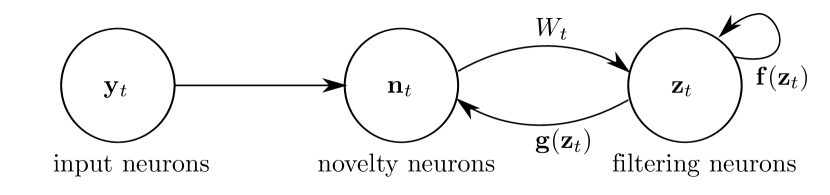
Figure 4: Neural Network Implementation. Implementation of Eq. (4) as a recurrent neuronal network. Here, $\mathbf{y}_{t}$, $\mathbf{n}_{t}$ and $\mathbf{z}_{t}$ denote neuronal populations.

Hebbian learning

In this interpretation, $W$ corresponds to the matrix of synaptic weights that connects novelty neurons $\mathbf{n}$ to filtering neurons $\mathbf{z}_{t}^{(i)}$. If the generative function $\mathbf{g}(\mathbf{x}_{t})=J\mathbf{x}_{t}$ is linear, then $J$ denotes the matrix of feedback weights which connects filtering neurons to novelty neurons. In general, the learning rules for these weights are not local, i.e. they rely on the state of the whole network (cf. Eqs. 22 and 24). However, in the deterministic limit the learning rule for the generative weight matrix can be replaced by a learning rule that is both Hebbian and local and relies on a multiplication between pre- and postsynaptic activity (Eq. 12 and, more generally, Eq. 26, see Methods). Further, for small observation noise, $W_{t}$ can be replaced by a constant matrix without affecting the filtering performance. Therefore, at least in this limit, the network presented in Fig. 4 is implementable as a neuronal dynamics of a recurrent network with local Hebbian synaptic plasticity.

The NPF alleviates the ‘curse of dimensionality’.

In our example the frog had to estimate only a single hidden state, namely the one-dimensional position of the insect. In a more realistic setting, there is a large number of hidden states, ranging from the position of an object in three-dimensional space to the relative presence of a features making up a visual scene. Therefore, any filtering algorithm employed by a neuronal population in the brain should be economical in its resources, i.e. the number of neurons needed to solve the filtering task to a certain performance level should scale well with the number of hidden variables. The NPF, in particular when the decoding weight $W_{t}$ is determined with maximum likelihood, is able to solve the filtering task in higher dimensions with just a limited number of filtering neurons. It thus alleviates the curse of dimensionality, which would be devastating for a realistic implementation.

We want to illustrate this point numerically with a toy example comparing the filtering performance of the NPF in terms of its MSE for very small number of particles to that of a standard PF (Fig. 5). In general, we find that the NPF performs well even for a limited number of samples. If we further allow the NPF to learn its decoding weight matrix $W_{t}$ by maximum likelihood, the filter is able to solve the filtering task with a single particle almost as good as with more particles. On the other hand, in a single-particle scenario the NPF using $W_{t}=\text{cov}(\mathbf{x}_{t},\mathbf{g}(\mathbf{x}_{t}))\Sigma_{y}^{-1}$ as well as the standard particle filter unsurprisingly exhibit an MSE, which corresponds to an independent trajectory of the prior. Upon increasing the number of samples, the PF outperforms the NPF again, owing to the approximations employed by it. However, this crossover-point tends to move towards larger number of particles for higher dimensions (e.g. Fig. 5), which is also not surprising: The PF trajectories evolve according to the prior, and in higher dimensions only a few particles will be in the correct spatial domain fitting to the observation and will thus have a non-vanishing weight..

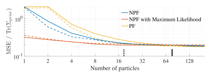
Figure 5: The NPF alleviates the ‘curse of dimensionality’. Toy example with nonlinear hidden dynamics and linear observation dynamics. Solid lines: $D=5$ hidden dimensions, dashed lines $D=1$ hidden dimensions for comparison. The error indicates the mean Euclidean distance of the estimated state $\langle\mathbf{x}_{t}\rangle$ from the real hidden state $\mathbf{x}_{t}$, normalized by the trace of the prior variance to make the error dimension-free. The black marker indicates the approximate cross-over point between the Neural Filter with gain matrix $W_{t}$ obtained by maximum likelihood and particle filter in $D=5$ (solid) and $D=1$ (dotted) hidden dimensions, which tends to move towards larger particle numbers as the dimensionality grows. Note that the number of filtering neurons is not equal to the number of particles $N$, but rather to $D\cdot N$.

The robustness of performance for smaller number of particles, which we observe in the NPF, is mainly due to the direct influence of the observations $d\mathbf{y}_{t}$ on the trajectories of the samples that correspond to the neuronal activities. In the NPF, each neuronal activity itself can be seen as a ”mini approximation” of the true posterior in terms of a $\delta$-function, an approximation which becomes exact for very small observation noise $\Sigma_{y}$. Of course, the larger $\Sigma_{y}$ becomes, the less the true posterior resembles a $\delta$-function and the more particles are needed to account for its shape in general.

Discussion

In this paper, we formulated the computational task of nonlinear Bayesian filtering. Based on the theory of nonlinear filtering, we proposed an Itô SDE for the posterior process and derived a learning rule for the parameters of this filter itself as well as for the generative weights of the underlying generative model. We have thus put forward an algorithm that allows for approximate filtering in continuous time for continuous-valued hidden processes. This algorithm allows the hidden dynamics as well as the observation dynamics to be nonlinear, and thus our model is flexible in representing a large class of general signal and emission statistics. The sampling-based framework is a central aspect of our NPF and as such is well in line with the ‘Neural sampling hypothesis’ [33].

Besides being an ansatz that is broadly consistent with neuronal dynamics, the neural filter equation we propose in Eq. (4) is particularly suited to model perception phenomenologically, because it shares some important properties with perception. First, perception relies on noisy and incomplete sensory data, and uses these to make sense of the world, which in our model is reflected by inferring the hidden state variable. Second, because prior dynamics directly enter the neuronal dynamics, prior knowledge about the environment is automatically incorporated and can in principle be learned. Third, information from different sensory modalities is efficiently combined as a weighted input to the population of filtering neurons. Lastly, perception can adapt to changes in the environment, which is taken into account by a dynamical gain and online parameter updates.

The implementation on a biologically realistic architecture imposes constraints on the algorithm itself as well as on how we can interpret its elements and structure. We should always be aware that these constraints describe a highly simplified version of the real biological underpinning, but have successfully been applied in network models to qualitatively understand core computations in the brain [36, p. 229ff]. First, neurons communicate among each other via discrete spikes, i.e. a digital signal. In contrast, we use the term ‘neuronal activity’ to denote an analog quantity. In some cases, for instance for a large number of neurons [36, p. 231], this ‘analog quantity’ may for instance correspond to an instantaneous firing rate. To take into account ‘negative’ neuronal activities, we could also consider deviations from a baseline firing rate or the membrane potential of the neuron, or the logarithm of the firing rate. Secondly, computations in and between neurons are performed through a weighted sum of inputs from cells they are connected to, and these inputs may be a (nonlinear) transformation of the presynaptic activity. Third, a hallmark of neural circuits is the synaptic connectivity between the neurons, the connection strength of which quantified by connective weights. These synaptic weights are modified by learning rules, which in the most simple case are local, i.e. they depend on the pre- and the postsynaptic neuronal activity. The learning rules in our model are in general not local, and in fact, each filter neuron $z^{(k)}$ has to know about the state of every other filter neuron and/or novelty neuron. Apart from that, when parameters are learned online, it is not clear how the filter derivative should be implemented in the network. However, we have shown that the learning rules of our model become both Hebbian and local for small observation noise, making these learning rules biologically plausible in this limit. Lastly, because the number of neurons in the brain is finite, computations clearly have to rely on a finite number of neurons, a fact we are taking into account by representing probability distributions with samples. Because these requirements are met by our proposed network structure, we consider our neuronal dynamics for filtering to be in line with standard network models.

Comparison to related work

The NPF is a filtering algorithm for a continuous-time continuous-state generative model with nonlinear hidden and observation dynamics. Filtering algorithms based on linear generative models have been subject to extensive research. and mainly study how the analytical solution to this problem, the Kalman filter, can be implemented with neurons (e.g. [11, 37, 12, 31]). However, the posterior resulting from a Kalman filter is always Gaussian, which is highly restrictive and does not properly reflect activity distributions observed in neurons (compare for instance the observations related to sparse coding as in [38]). Unlike the various extensions of the Kalman filter [13] – such as the EKF or the unscented Kalman filter [39] – which are applied to nonlinear systems, the NPF is not restricted to approximate the posterior by a Gaussian parametrized by its first and second moment. Rather, due to the nonlinearity in the network dynamics it may represent any probability distribution at any given time step.

An important aspect of our work is the sampling-based representation of probability distributions, whereby the activity of each neuron is considered a single sample. There are two main competing proposals about how the probability distributions underlying Bayesian computations might be represented in the brain. Firstly, it has been suggested that probability distributions are expressed as probabilistic population codes (PPC [40]), in which each neuron represents a state of the encoded random variable and their activities are proportional to the probability of the corresponding state. Filtering approaches based on population codes, in which the neuronal activity directly relates to the posterior or the log posterior, have been explored in the literature for a large set of models, e.g. [11, 41, 42, 12]. In this representation, neurons directly correspond to the parameters of the distribution, and thus the critical factor for accuracy is the number of neurons. Further, they all suffer from the ‘curse of dimensionality’ for multimodal distribution. The second proposal, called neural sampling hypothesis [33], uses an inference scheme where the activity of each neuron represents a sample from the underlying probability distribution. Since our filtering algorithm is based on unweighted samples, our findings are in line with the advantages of the sampling-based representation outlined in [33]: it can represent any distribution without the need for a parametric form, it mitigates the ‘curse of dimensionality’ and it is well-suited for learning. Filtering approaches implementing Markov-chain Monte Carlo (MCMC) algorithms have received some attention lately [43, 44], but since they rely on a discrete state space and assume a different coding scheme than the one suggested in [33], the advantages listed there do not necessarily emerge from these models.

As a filtering algorithm, the NPF is well in accordance with existing sample-based filtering approaches. Our ansatz may be seen as a particle filter where all particles carry the same weight and which, therefore, avoids numerical pitfalls such as weight degeneracy. This problem is notorious in standard MCMC particle filters [18] and becomes even more severe as the number of hidden dimensions grows. The curse of dimensionality, i.e. the exponential growth of approximation error with the dimension of the underlying model, is an inevitable nuisance in standard MCMC approaches. There are some tricks to deal with these problems, for instance by particle resampling or using a more refined propagator for the particles (like the optimal importance function in [18]), but neither solution is able to properly circumvent weight decay in general. Moreover, there is currently no proposed implementation of weighted particle methods in a neural architecture. For instance, the need to renormalize the weights at each time step introduces a coupling between the particles: While their trajectories are independent, their weights are certainly not. On the other hand, the neural filter, not relying on importance weights in the first place, does not suffer from these numerical pitfalls and their related implementational issues. The curse of dimensionality seems to be avoided, or at least mitigated, by the fact that the observations directly enter the particle trajectories. However, the particles following the NPF dynamics are not completely independent either. Coupling between the particles is mediated by the decoding weight matrix $W_{t}$, whose learning rule is influenced by all the particles. This could be avoided by fixing $W_{t}$ to a constant consistent with observational noise $\Sigma_{y}$, e.g. after learning. Even if it is numerically a bit off what we think the ‘real’ decoding weight should be, the filtering performance is not seriously affected and particle trajectories are effectively decoupled.

In the literature, there have been other approaches for particle filtering without importance weights, derived rigorously from mathematical filtering theory [45, 46]. One of these approaches, the so-called feedback particle filter [45], is based on a similar SDE for the particle trajectories as the one we propose in Eq. (4). It can be shown that the underlying distribution of the feedback particle filter evolves exactly according to the Kushner equation, whereas our approach merely approximates it. However, the computation of the gain function in the feedback particle filter needs access to the full filtering distribution itself, and in order to avoid numerical issues their algorithm relies on a regularization scheme that would be hard to justify biologically. Though formally a multivariate version of the feedback particle filter exists, the gain function cannot be solved for in closed form. The Neural Filter, though not an exact particle algorithm, overcomes this drawback by being readily applicable in higher dimensions and by being comparatively easy to compute.

The neuronal network structure (Fig. 4) we propose to implement the neuronal dynamics according to Eq. (4) is structurally similar to the one proposed in [9]. As in their model, we represent neuronal activities in terms of their instantaneous firing rate, which is an approximation to the spiking nature of biological neurons. In their predictive coding model, a central role is assigned to the predictive error signal, which can be compared to the dynamics of the novelty neurons or novelty signal $d\mathbf{n}_{t}$ in our model. Accordingly, equations for the neuronal dynamics and for learning the generative weight in the small observation noise limit is structurally similar. However, our model generalizes the one in [9] in the sense that we allow dynamics in the prior, which is directly reflected in the dynamics of the filtering neurons.

Implications

The three central aspects of our work, namely a sampling-based representation, a filtering algorithm with adaptive gain and the structure of the recurrent neuronal network, result in the following implications for the neuronal network:

1. The network is robust against neuronal failure.

2. An internal model about the world becomes manifest in internal neuronal dynamics

3. Neuronal variability is tuned according to sensory reliability.

4. Neurons may code for the novelty given by discrepancy between prediction by an internal model and actual observations.

The first implication follows directly from the sampling-based representation, namely robustness against neuronal failure. For example, if a distribution is represented by 1000 particles, removing 10% will not significantly decrease the ability of the other particles to represent the probability distribution. In an extreme case, we could consider a single neuron to represent the whole distribution, given that its activity state can take values in the same range as the hidden state and we allow it to sample the distribution in time. Apart from that, as we have seen numerically, the ability to perform filtering with a reduced number of particles is not affected by particle removal to a large extent either, at least not in the particular algorithm we propose. However, some degree of plasticity or rewiring would be necessary in order to read out expectations from the decimated neuronal population. On the other hand, in parametric representations such as a PPC, where each neuron determines the height of a particular tuning curve assigned to it and that actually rely on the tuning curves to cover the space densely [40], neuronal failure can be devastating: With each neuron that breaks down, a particular point in state space cannot be represented directly anymore. Clearly, a single neuron would never be able to account for any other distribution than the one resembling its own tuning curve.

The second and third implication is a consequence of the adaptive gain, i.e. the decoding weight $W_{t}$, that determines the emphasis that is laid on new observations. As we have demonstrated, the gain $W_{t}$ in our model increases with sensory reliability both according to sensory noise and ambiguity in the input generation, putting more emphasis on the observations versus its internal model. In the absence of observations, observation noise is maximal and the neuronal dynamics follow those of the hidden state which comprises an internal model about the world. With availability of observations, sensory reliability naturally increases and variability across samples should decrease, because now their dynamics are influenced by the same stimulus via the gain $W_{t}$. Indeed, it has been found that spontaneous neuronal activities relate to prior expectations about a stimulus in visual cortex [32]. Further, it has been shown that inter-trial variability of neuronal responses declines upon stimulus onset [7]. Both these experimental findings are nicely in line with our theoretical predictions.

Conclusion and Outlook

With the Neural Particle Filter we have come up with an algorithm that allows neurons to perform nonlinear Bayesian filtering in a sampling-based manner. Specifically, the neuronal implementation is based on a network of recurrently connected analog neurons whose dynamics are governed by the NPF algorithm. In future work, the biological plausibility of this recurrent network model will be further addressed. First, observing that the learning rules in general, i.e. for nonvanishing observation noise, do not fulfill the requirement of locality, which is needed for a biologically plausible learning rule (e.g. a Hebbian learning rule), the model could be enhanced such that individual filtering neurons obey different rather than identical dynamics. We could for instance consider $N$ different subnetworks and locally determine the weights in these subnetworks, possibly taking into account a (slowly-changing) global modulation factor. Such an approach would also effectively decouple the particles on a smaller timescale. Second, by including the theory of filtering and identification of point processes, our algorithm could be extended such that a spike-based representation may be accounted for.

Methods

Details on numerical experiments

The choice of the decoding weight $W_{t}$

In our numerical simulations, we consider and compare two choices of the decoding weight $W_{t}$, which we will quickly motivate here.

As a first choice, we consider $W_{t}=\text{cov}(\mathbf{x},\mathbf{g}(\mathbf{x})^{T})\Sigma_{y}^{-1}$, a choice inspired by the dynamics of the formal solution. In particular, consider the dynamics of the first posterior moment, which by comparison with the NPF equation (Eq. 4) directly motivates this particular choice of the decoding weights. Thereby, the covariance $\text{cov}(\mathbf{x},\mathbf{g}(\mathbf{x})^{T})$ is estimated empirically from the samples $\mathbf{z}_{t}^{(k)}$via

$$\text{cov}(\mathbf{x},\mathbf{g}(\mathbf{x})) \approx \frac{1}{N}\sum_{k=1}^{N}\mathbf{z}_{t}^{(k)}\mathbf{g}(\mathbf{z}_{t}^{(k)})^{T}-\frac{1}{N^{2}}\sum_{k,l=1}^{N}\mathbf{z}_{t}^{(k)}\mathbf{g}(\mathbf{z}_{t}^{(l)})^{T}.$$ (13)

As a second choice, we consider $W=W_{\text{ML}}$, i.e. the decoding weight $W_{t}$ and thus the Neural Filter itself is tuned via maximum likelihood. The learning rule is given in Eq. (22) and corresponds to an online update of the decoding weight at each time step. What is peculiar about this choice is that here a decoding rather than a generative model parameter is learned, illustrating that inference and learning can be very intertwined: In fact, it is actually possible to rephrase the filtering problem in terms of a learning problem by giving an ansatz for a decoder whose parameters have to be learned such that it can perform filtering, but we will not consider this rather extreme case here.

Dynamics and parameters

For our simulations, we use a nonlinear hidden dynamics, that was chosen to have a bimodal stationary distribution:

$$dx_{t} = ax_{t}(b-x_{t}^{2})\,dt+\sigma_{x}d\omega_{t}.$$ (14)

The parameters $a>0$ and $b>0$ can be used to tune the shape of the bimodal distribution, whereby the positions of the two modes is determined by $\pm b$ and $a$ defines how sharply the distribution is peaked around the modes. Unless stated otherwise, parameters for the deterministic dynamics were $a=3$ and $b=1$, resulting in a bimodal distribution with distinct, but not too sharp peeks at $\pm 1$, such that it is possible for the hidden state to switch from one mode to the other.

In our examples in Fig. 1, we employ both linear and sigmoid observation dynamics $g(x)$, thereby simulating multisensory integration with our model (cf. Eqs. 8 and 7). For the plots in Fig. 2, we use only one sensory modality per row. The observation noise $\sigma_{v}$ and $\sigma_{a}$ is varied between $10^{-4}$ and $300$.

In the multidimensional simulations in Fig. 5, the hidden dynamics within each dimension is independent of the other dimensions and and corresponds to Eq. (14), with $\Sigma_{x}$ chosen to be the unit matrix. The stationary distribution of this dynamics is thus a multimodal distribution with $2^{n}$ peaks for $n$ dimensions. The linear generative function is given by $\mathbf{g}(\mathbf{x})=J\mathbf{x}$ with $J$ a rotation matrix rotating the hidden state vector by 30 degrees around each spatial axis. In the simulations shown in Fig. 5, $\Sigma_{y}=0.1\cdot\mathbb{I}$.

Mean-squared errors (MSE) and biases of estimated quantities or parameters $\hat{\theta}$ were computed by

$$MSE = \frac{1}{T}\sum_{t=1}^{T}|\mathbf{x}_{t}-\langle\mathbf{x}\rangle|^{2},$$ (15)

$$Bias(\hat{\theta}) = \frac{1}{T}\sum_{t=1}^{T}\hat{\theta}_{t}-\theta_{t},$$ (16)

where $\theta_{t}$ denotes the true or benchmark (particle filter) value. Unless stated otherwise, MSEs are normalized with respect to the trace of the stationary prior variance $\Sigma_{prior}$ to make performance comparable and, if needed, independent of the number of hidden dimensions.

Other simulation parameters comprise the time step size, which was set to $dt=0.005$ throughout all simulations. All simulations were run for 500’000 time steps, corresponding to 2500 time units. Unless stated otherwise, MSEs and biases were averaged over the last 1000 time units, equaling 200’000 time steps.

Benchmark models

We would like to stress that the generative model we chose in our examples are nonlinear both in prior as well as in observation dynamics. This implies that a closed form solution to this problem does not exist, and thus approximations have to be employed. Therefore, when assessing the performance of the NPF, we compare it to two approximate filtering algorithms, both of which widely used in approximating the posterior distribution in nonlinear filtering problems: a standard particle filter [18] and continuous-time version of the extended Kalman filter [26]. For further information on these algorithms, see S1 Appendix..

Maximum likelihood parameter learning

The cost function

For the continuous-time continuous state-space generative model given by Eqs. (1) and (2), learning in the mathematical literature commonly referred to as ‘system identification’, is a tough problem which has hardly been looked at. In fact, the (to our knowledge) only reference which gives an explicit cost function for identification in our setting is a technical report by Moura and Mitter [47]. Based on a change of probability measure, they propose a cost function that is equivalent to the log likelihood of the input $\log p_{\theta}(\mathcal{Y}_{t})$ with model parameters $\theta$, which for our model reads:

$$L_{t}^{\text{offline}}(\theta)=\int_{0}^{t}\langle\mathbf{g}(\mathbf{x}_{s})\rangle^{T}\Sigma_{y}^{-1}\,d\mathbf{y}_{s}-\frac{1}{2}\langle\mathbf{g}(\mathbf{x}_{s})\rangle^{T}\Sigma_{y}^{-1}\langle\mathbf{g}(\mathbf{x}_{s})\rangle\,ds,$$ (17)

where expectations are taken with respect to the filtering distribution at time $s$, $p(\mathbf{x}_{s}|\mathcal{Y}_{s})$.

In a discrete-time approximation, Eq. (17) immediately suggests an online maximization scheme. Instead of maximizing the cost function at a time $t$ for the whole observation sequence $\mathcal{Y}_{t}$, implying we would have to run the filter all over again each time we change the parameters, we just perform a gradient ascent with respect to the parameters $\theta$ on the last contribution to the integral, i.e. to

$$L^{\text{online}}_{t}(\theta)=\langle\mathbf{g}(\mathbf{x}_{t})\rangle^{T}\Sigma_{y}^{-1}\,d\mathbf{y}_{t}-\frac{1}{2}\langle\mathbf{g}(\mathbf{x}_{t})\rangle^{T}\Sigma_{y}^{-1}\langle\mathbf{g}(\mathbf{x}_{t})\rangle\,dt,$$ (5)

where expectations are with respect to the filtering distribution at time $t$, $p(\mathbf{x}_{t}|\mathcal{Y}_{t})$. It can be shown that maximization of this cost function is equivalent to a minimization of the reconstruction error $(d\mathbf{y}_{t}-\mathbf{g}(\mathbf{x}_{t})\,dt)^{2}$ at each time step (see S1 Appendix. for a proof).

Learning rules

Parameter learning is implemented by maximizing the log likelihood (Eq. 5) by a gradient ascent with respect to the model parameters $\theta$, giving rise to the following online learning rule for the parameters:

$$\eta_{\theta}^{-1}\Delta\theta = \Big{(}\frac{\partial}{\partial\theta}\langle\mathbf{g}(\mathbf{x}_{t})\rangle\Big{)}^{T}\Sigma_{y}^{-1}\big{(}d\mathbf{y}_{t}-\langle\mathbf{g}(\mathbf{x}_{t})\rangle\,dt\big{)}.$$ (18)

This approximation of learning is justified if the time scale of learning is much larger than the dynamics of the filter, i.e. for small learning rates.

Equation (18) exhibits a peculiar structure: The novelty signal $d\mathbf{y}_{t}-\langle\mathbf{g}(\mathbf{x}_{t})\rangle\,dt$ is multiplied with a parameter gradient on the posterior estimate of the generative function $\langle\mathbf{g}(\mathbf{x}_{t})\rangle$. Thus, we have to take into account the implicit change of the posterior distribution, the so called filter derivative, with respect to the model parameters. The filter derivative is in general hard or even impossible to compute analytically and many identification problems deal with estimating it (cf. for instance [19, 35]).

In our model, we make use of the approximated posterior dynamics in order to derive dynamics of the filter derivative for parameter learning. Equation 18 can be approximated by taking $N$ samples from the NPF equation (4) in order to express the posterior estimates:

$$\langle\mathbf{g}(\mathbf{x}_{t})\rangle \approx \frac{1}{N}\sum_{k=1}^{N}\mathbf{g}(\mathbf{z}_{t}^{(k)}),$$ (19)

$$\frac{\partial}{\partial\theta}\langle\mathbf{g}(\mathbf{x}_{t})\rangle \approx \frac{1}{N}\sum_{k=1}^{N}G(\mathbf{z}_{t}^{(k)})\frac{\partial\mathbf{z}_{t}^{(k)}}{\partial\theta},$$ (20)

where $G_{ij}(\mathbf{z}^{(k)})=\frac{\partial g_{i}}{\partial x_{j}}(\mathbf{z}^{(k)})$ denotes the Jacobian of the generative function. Thus, the filter derivative is taken into account by considering the infinitesimal change in the position of sample $\mathbf{z}^{(k)}$ with respect to the change in parameter value $\theta$.

The single particle filter derivative, $\frac{\partial\mathbf{x}_{t}^{(k)}}{\partial\theta}$, cannot be computed directly. However, based on Eq. (4), it is possible to compute its dynamics:

$$d\left(\frac{\partial\mathbf{z}_{t}^{(k)}}{\partial\theta}\right) = \frac{\partial}{\partial\theta}\big{(}d\mathbf{z}_{t}^{(k)}\big{)}.$$ (21)

Note that every single parameter that is learned has $N$ accompanying filter derivatives of this form.

In this work we are interested in learning the decoding weight matrix $W_{t}$ and, for a linear observation dynamics $\mathbf{g}(\mathbf{x})=J\mathbf{x}$, in learning the generative matrix J, respectively. The resulting learning rules for the components of the decoding weight matrix with learning rate $\eta_{W}$ are given by

$$\Delta W_{ij} = \eta_{W}\frac{\partial}{\partial_{W_{ij}}}\langle\mathbf{g}(\mathbf{x}_{t})\rangle^{T}\Sigma_{y}^{-1}\left(d\mathbf{y}_{t}-\langle\mathbf{g}(\mathbf{x}_{t})\rangle dt\right),$$ (22)

with filter derivative dynamics

$$d\left(\frac{\partial\mathbf{z}_{t}^{(k)}}{\partial W_{ij}}\right) = \left(F(\mathbf{z}_{t}^{(k)})-WG(\mathbf{z}^{(k)}_{t})\right)\frac{\partial\mathbf{z}_{t}^{(k)}}{\partial W_{ij}}dt+\big{[}d\mathbf{y}_{t}-\mathbf{g}(\mathbf{z}^{(k)}_{t})dt\big{]}_{j}\mathbf{e}_{i},$$ (23)

where $F_{ij}(\mathbf{z}^{(k)})=\frac{\partial f_{i}}{\partial x_{j}}(\mathbf{z}^{(k)})$ denotes the Jacobian of the nonlinear hidden dynamics and $\mathbf{e}_{i}$ denotes the unit vector in the $i$-th direction. This implies that, when we take $W_{t}$ to be a plastic decoding weight matrix that is learned as observations become available, at least three equations are needed to infer the hidden state at each time step: First, Eq. (4) to evolve the states of the filter neurons, and second, Eqs. (22) and (23) to update the weights in the filter equation.

Analogously, learning rules for the components of the generative matrix for linear observation dynamics $\mathbf{g}(\mathbf{x})=J\mathbf{x}$ read

$$\Delta J_{ij} = \eta_{J}\left[\left(\frac{\partial\langle\mathbf{x}_{t}\rangle}{\partial J_{ij}}\right)^{T}J^{T}\Sigma_{y}^{-1}(d\mathbf{y}_{t}-J\langle\mathbf{x}_{t}\rangle\,dt)+\Big{(}\Sigma_{y}^{-1}(d\mathbf{y}_{t}-J\langle\mathbf{x}_{t}\rangle\,dt)\Big{)}_{ij}\right].$$ (24)

In addition to a term proportional to the filter derivative, the learning rule contains a second term that emerges from an explicit dependence of the likelihood in the generative weight. Filter derivatives are given by

$$d\left(\frac{\partial\mathbf{z}_{t}^{(k)}}{\partial J_{ij}}\right) = \left(F(\mathbf{z}_{t}^{(k)})-WJ\right)\frac{\partial\mathbf{z}_{t}^{(k)}}{\partial J_{ij}}dt-\hat{x}_{t,j}^{(k)}W\mathbf{e}_{i}dt.$$ (25)

Bias due to sampling

In the derivation of these learning rules, we used a sampling-based representation of the approximated posterior in order to estimate log-likelihood and gradients. This introduces a bias in these estimations, which we should correct for when computing parameter estimates. Unfortunately, this bias is in general not analytically accessible, but at least for a linear generative model it can be shown that it vanishes with $1/N$ (for a proof, see S1 Appendix.).

Approximation for small observation noise

The learning rules we obtain for the decoding weights $W_{t}$ and the generative weights $J$ are not local, implying that the weights can only be computed when knowing the state of each filter neuron at each time. However, for small observation noise the learning rule for the generative weight $J$ can be approximated by a local learning rule with a Hebbian structure. First, we can neglect the filter derivative, which decays to zero very fast because in this limit, the decoding weight $W_{t}$ is generally large (cf. Eq. 25), and thus the first term in Eq. (24) vanishes. Second, because in this limit the posterior will approach a $\delta$-distribution around the true hidden state $\mathbf{x}$, as does the approximated posterior, we can approximate the learning rule for $J$ by:

$$\eta_{J}^{-1}\Delta J \propto (d\mathbf{y}_{t}-J\langle\mathbf{x}_{t}\rangle\,dt)\langle\mathbf{x}_{t}\rangle^{T}\approx\langle(d\mathbf{y}_{t}-J\mathbf{x}_{t})\mathbf{x}_{t}^{T}\rangle,$$ (26)

which takes the form of a local Hebbian learning rule.

Supporting Information

S1 Appendix.

The Neural Particle Filter: Mathematical Appendix.

References

- 1. Knill DC, Pouget A. The Bayesian brain: the role of uncertainty in neural coding and computation. Trends in Neurosciences. 2004;27(12):712–719. doi:10.1016/j.tins.2004.10.007.
- 2. Doya K, Ishii S, Pouget A, Rao RPN. Bayesian Brain: Probabilistic Approaches to Neural Coding. The MIT Press; 2007.
- 3. Wolpert D, Ghahramani Z, Jordan M. An internal model for sensorimotor integration. Science. 1995;269(5232):1880–1882. doi:10.1126/science.7569931.
- 4. Körding KP, Wolpert DM. Bayesian integration in sensorimotor learning. Nature. 2004;427(January):244–247. doi:10.1038/nature02169.
- 5. Ernst MO, Banks MS. Humans integrate visual and haptic information in a statistically optimal fashion. Nature. 2002;415(6870):429–433. doi:10.1038/415429a.
- 6. Churchland AK, Kiani R, Chaudhuri R, Wang XJ, Pouget A, Shadlen MN. Variance as a signature of neural computations during decision making. Neuron. 2011;69(4):818–831. doi:10.1016/j.neuron.2010.12.037.
- 7. Churchland MM, Yu BM, Cunningham JP, Sugrue LP, Cohen MR, Corrado GS, et al. Stimulus onset quenches neural variability: a widespread cortical phenomenon. Nature Neuroscience. 2010;13(3):369–378. doi:10.1038/nn.2501.
- 8. Orbán G, Berkes P, Fiser J, Lengyel M. Neural Variability and Sampling-Based Probabilistic Representations in the Visual Cortex. Neuron. 2016;92(2):530–543. doi:10.1016/j.neuron.2016.09.038.
- 9. Rao RPN, Ballard DH. Predictive coding in the visual cortex: a functional interpretation of some extra-classical receptive-field effects. Nature Neuroscience. 1999;2(1):79–87. doi:10.1038/4580.
- 10. Huang Y, Rao RPN. Bayesian Inference and Online Learning in Poisson Neuronal Networks. Neural Computation. 2016;28(8):1503–1526.
- 11. Denève S, Duhamel JR, Pouget A. Optimal sensorimotor integration in recurrent cortical networks: a neural implementation of Kalman filters. The Journal of neuroscience : the official journal of the Society for Neuroscience. 2007;27(21):5744–5756. doi:10.1523/JNEUROSCI.3985-06.2007.
- 12. Makin JG, Dichter BK, Sabes PN. Learning to Estimate Dynamical State with Probabilistic Population Codes. PLoS Computational Biology. 2015;11(11):1–28. doi:10.1371/journal.pcbi.1004554.
- 13. Kalman RE. A New Approach to Linear Filtering and Prediction Problems. Transactions of the ASME Journal of Basic Engineering. 1960;82(Series D):35–45. doi:10.1115/1.3662552.
- 14. Kalman RE, Bucy RS. New Results in Linear Filtering and Prediction Theory. Journal of Basic Engineering. 1961;83(1):95. doi:10.1115/1.3658902.
- 15. Kording KP, Tenenbaum JB, Shadmehr R. The dynamics of memory as a consequence of optimal adaptation to a changing body. Nature Neuroscience. 2007;10(6):779–786. doi:10.1038/nn1901.
- 16. Kushner H. On the Differential Equations Satisfied by Conditional Probability Densities of Markov Processes, with Applications. Journal of the Society for Industrial & Applied Mathematics, Control. 1962;2(1).
- 17. Zakai M. On the optimal filtering of diffusion processes. Zeitschrift für Wahrscheinlichkeitstheorie und verwandte Gebiete. 1969;243.
- 18. Doucet A, Godsill S, Andrieu C. On sequential Monte Carlo sampling methods for Bayesian filtering. Statistics and Computing. 2000;10(3):197–208. doi:10.1023/A:1008935410038.
- 19. Kantas N, Doucet A, Singh SS, Maciejowski J, Chopin N. On Particle Methods for Parameter Estimation in State-Space Models. Statistical Science. 2015;30(3):328–351. doi:10.1214/14-STS511.
- 20. Welling M, Teh YW. Bayesian Learning via Stochastic Gradient Langevin Dynamics. In: Proceedings of the 28th International Conference on Machine Learning; 2011.
- 21. MacKay DJ. Information Theory, Inference and Learning Algorithms. Cambridge University Press; 2005.
- 22. Hennequin G, Aitchison L, Lengyel M. Fast Sampling-Based Inference in Balanced Neuronal Networks. Advances in Neural Information Processing Systems. 2014;.
- 23. Moreno-Bote R, Knill DC, Pouget A. Bayesian sampling in visual perception. Proceedings of the National Academy of Sciences of the United States of America. 2011;108(30):12491–12496. doi:10.1073/pnas.1101430108.
- 24. Kappel D, Habenschuss S, Legenstein R, Maass W. Network Plasticity as Bayesian Inference. PLoS Computational Biology. 2015;11(11):1–31. doi:10.1371/journal.pcbi.1004485.
- 25. Marr D. Vision - A Computational Investigation into the Human Representation and Processing of Visual Information. WH Freeman & Co. San Francisco; 1982.
- 26. Jazwinski AH. Stochastic Processes and Filtering Theory. Bellman R, editor. New York: Academic Press; 1970.
- 27. Bain A, Crisan D. Fundamentals of Stochastic Filtering. New York: Springer; 2009.
- 28. Doucet A, Johansen A. A tutorial on particle filtering and smoothing: Fifteen years later. Handbook of Nonlinear Filtering. 2009.
- 29. Crisan D, Rozovskii B, editors. No Title. 1st ed. Oxford University Press; 2011.
- 30. Daum F, Huang J. Curse of Dimensionality and Particle Filters. Proceedings of the IEEE Aerospace Conference. 2003;4:1979–1993. doi:10.1109/AERO.2003.1235126.
- 31. Greaves-Tunnell A. An optimization perspective on approximate neural filtering; M.Sc. Thesis, University of Cambridge. 2015.
- 32. Berkes P, Orban G, Lengyel M, Fiser J. Spontaneous Cortical Activity Reveals Hallmarks of an Optimal Internal Model of the Environment. Science. 2011;331(6013):83–87. doi:10.1126/science.1195870.
- 33. Fiser J, Berkes P, Orbán G, Lengyel M. Statistically optimal perception and learning: from behavior to neural representations. Trends in Cognitive Sciences. 2010;14(3):119–130. doi:10.1016/j.tics.2010.01.003.
- 34. Lo JT, Yu L. Recursive neural filters and dynamical range transformers. Proceedings of the IEEE. 2004;92(3):514–535. doi:10.1109/JPROC.2003.823148.
- 35. Surace SC, Pfister JP. Online Maximum Likelihood Estimation of the Parameters of Partially Observed Diffusion Processes. 2016;(3):1–10.
- 36. Dayan P, Abbott LF. Theoretical Neuroscience: Computational and Mathematical Modeling of Neural Systems. Computational Neuroscience Series. Massachusetts Institute of Technology Press; 2001.
- 37. Wilson RC, Finkel L. A neural implementation of the Kalman filter. Advances in Neural Information Processing Systems. 2009;22.
- 38. Olshausen BA, Field DJ. Emergence of simple-cell receptive field properties by learning a sparse code for natural images. Nature. 1996;381(6583):607–9. doi:10.1038/381607a0.
- 39. Julier SJ, Uhlmann JK. A New Extension of the Kalman Filter to Nonlinear Systems. System Identification. 1997;3:3–2. doi:10.1117/12.280797.
- 40. Ma WJ, Beck JM, Latham PE, Pouget A. Bayesian inference with probabilistic population codes. Nature neuroscience. 2006;9(11):1432–8. doi:10.1038/nn1790.
- 41. Beck JM, Pouget A. Exact inferences in a neural implementation of a hidden Markov model. Neural computation. 2007;19(5):1344–1361. doi:10.1162/neco.2007.19.5.1344.
- 42. Sokoloski S. Implementing a Bayes Filter in a Neural Circuit: The Case of Unknown Stimulus Dynamics. ArXiv. 2015;.
- 43. Pecevski D, Buesing L, Maass W. Probabilistic inference in general graphical models through sampling in stochastic networks of spiking neurons. PLoS Computational Biology. 2011;7(12). doi:10.1371/journal.pcbi.1002294.
- 44. Legenstein R, Maass W. Ensembles of Spiking Neurons with Noise Support Optimal Probabilistic Inference in a Dynamically Changing Environment. PLoS computational biology. 2014;10(10):e1003859. doi:10.1371/journal.pcbi.1003859.
- 45. Yang T, Mehta PG, Meyn SP. Feedback particle filter. IEEE Transactions on Automatic Control. 2013;58(10):2465–2480. doi:10.1109/TAC.2013.2258825.
- 46. Crisan D, Xiong J. Approximate McKean–Vlasov representations for a class of SPDEs. Stochastics An International Journal of Probability and Stochastic Processes. 2010;82(1):53–68. doi:10.1080/17442500902723575.
- 47. Moura JMF, Mitter SK. Identification and Filtering: Optimal Recursive Maximum Likelihood Approach; MIT Technical Report. 1986