A Modified Quadratic Lorenz Attractor

Abstract.

This study introduces a modified quadratic Lorenz attractor. The properties of this new chaotic system are analysed and discussed in detail, by determining the equilibria points, the eigenvalues of the Jacobian, and the Lyapunov exponents. The numerical simulations, the time series analysis, and the projections to the $xy$-plane, $xz$-plane, and $yz$-plane are conducted to highlight the chaotic behaviour. The multiplicative form of the new system is also presented and the simulations are conducted using multiplicative Runge-Kutta methods.

1. Introduction

Dynamical systems are mathematical models describing the evolution of systems in terms of equation of motion with sensitive initial values. The application areas of dynamical systems can be found e.g. in many disciplines in physics [24, 16, 2], population dynamics in biology [32], and chemical kinetics in chemistry [29, 25]. Dynamic systems theory has also found its way into subjects outside the fields of Mathematics and natural sciences, exemplarily we would like to mention mathematical economy and finance [14, 15, 20]. Poincaré made a kick start to the subject of dynamical systems in his pioneering work in 1890 [21]. Later, in the 1920’s, Fatou [8] and Julia [10] introduced the dynamics of complex analytic maps. On the one hand, studies like Birkhoff [3], Kolmogorov [13, 11, 12], Cartwright and Littlewood [4] find their origin in physics, like e.g. the three body problem in astronomy, whereas on the other hand Stephan Smale provided a purely mathematics motivated approach [27, 28]. E. N. Lorenz [16] observed that very simple differential equations become chaotic under certain circumstances. The system proposed by Lorenz shows a very complex dynamical behaviour and displays the well-known two-scroll butterfly-shape. The dynamic equations of the Lorenz system are given as

(1) $$\frac{dx}{dt} = \sigma(y-x),$$

(2) $$\frac{dy}{dt} = x(\rho-z)-y,$$

(3) $$\frac{dz}{dt} = xy-\beta z,$$

where the parameters $\sigma$, $\rho$, and $\beta$ are assumed to be positive. Lorenz used exemplarily the values $\sigma=10$, $\beta=8/3$ and $\rho=28$ to demonstrate the systems chaotic behaviour. The study on ”The equation for continuous chaos” by Rössler [24] can be seen as another landmark in the discussion of 3D dynamic systems. The Rössler system and the Burke Shaw system [26] have the property of two unstable saddle foci in common. Other chaotic systems exhibiting a similar simple structure as the Lorenz system, without being topologically equivalent, are proposed by Chen [5] and Lü and Chen [17]. [17] discusses the transition between Lorenz and Chen attractors. Furthermore, Yang and Chen introduced another chaotic system with three fixed points: one saddle and two stable fixed points. Yang et al. [30] and Pehlivan et al. [19] introduced and analysed chaotic systems similar to the Lorenz, Chen, and Yang-Chen systems, with two different fixed points, i.e. two stable node-foci. Chaotic systems have found their ways also into many applications in engineering, such as electronic circuits [7]-[31]. Modern pacemakers actually rely nowadays on these chaotic circuits.

Dynamical systems have also been discussed in the framework of various Non-Newtonian Calcului, like fractional calculus, geometric multiplicative calculus, and bigeometric multiplicative calculus. Jun Guo Lu transformed the Lü system into fractional calculus [18], investigating chaotic behaviour of fractional-order of the Lü system numerically. Aniszewska applied multiplicative calculus to the Rössler system and showed chaotic behaviour of multiplicative Rössler[1]. As an application of the bigeometric multiplicative Runge-Kutta method, the bigeometric multiplicative Rössler System was solved in [23].

This study introduces a new chaotic attractor, found by modification of the Lorenz system by a quadratic term. Detailed numerical and theoretical analysis reveals that the proposed system shows chaotic behaviour and the property of a two-scroll attractor like the Lorenz attractor.

Section 2 introduces the modified quadratic Lorenz attractor, discusses and analyses its properties by determining the equilibria points, and Lyapunov exponents theoretically as well as numerically. In Section 3, the modified quadratic Lorenz attractor is translated into geometric and bigeometric calculus, and the solutions of the the system are obtained using the corresponding multiplicative Runge-Kutta methods [22] and [23]. Finally, this paper closes with the summary of the obtained results.

2. Design of a new Chaotic System

This paper presents a new Chaotic system derived from the Lorenz system. The system is generated by the following simple three-dimensional system:

(4) $$\frac{dx}{dt} = \sigma(yz-x)$$

(5) $$\frac{dy}{dt} = \rho x-xz$$

(6) $$\frac{dz}{dt} = (xy)^{2}-\beta z$$

where $x$, $y$, and $z$ are variables and $\sigma$, $\rho$, and $\beta$ are real parameters. In the new proposed chaotic system, all the equations have some differences compared to the original Lorenz system. In order to see the differences between the two systems we can compare the equations (1)-(3) and (4)-(6) one by one. Evidently, in the Lorenz system equation (1) is linear, whereas equation (4) is non-linear. Furthermore, equations (2) and (5) are both non-linear, where the $y$-dependence of equation (5) is cancelled. The most significant difference can be observed comparing equations (3) and (6). In (6) the term $xy$ is squared compared to equation (3).

2.1. System Description

The initial values and the parameters of the system are chosen as $(1,1,1)$ and $\sigma=12$, $\rho=8$ with varying $\beta$. Then it has been observed that the behavior of the new chaotic system changes depending on the different values of $\beta$ as shown in Figure 1.

(a) $\beta=0.1$

(b) $\beta=0.5$

(c) $\beta=2$

(d) $\beta=4$

(e) $\beta=10$

Figure 1. Simulation of the system when $\sigma=12$, $\rho=8$ and various parameter values

As a result of the calculations, as it can be seen in Figure 1, it has been observed that the new system is chaotic for the parameters

(7) $$\sigma=12,\rho=8,\text{ and }\beta=4.$$

The analysis of the new chaotic system will be done according to those parameters.

2.2. System Analysis

The first step to analyze a chaotic system is to find the equilibrium points. In order to determine the equilibrium points of the proposed system (4)-(6), we need to solve the system

$$\sigma(yz-x) = 0$$

(8) $$\rho x-xz = 0$$

$$(xy)^{2}-\beta z = 0$$

Thus, the solution of the system (8) with respect to $x$, $y$, $z$ give the equilibria points as:

$$\it{O} = (0,0,0)$$

$$\it E^{+} = \left(\sqrt[4]{\beta\,\rho^{3}},\sqrt[4]{\frac{\beta}{\rho}},\rho\right)$$

$$\it E^{-} = \left(-\sqrt[4]{\beta\,\rho^{3}},-\sqrt[4]{\frac{\beta}{\rho}},\rho\right)$$

For the parameters chosen in (7), the numerical values of the equilibria points are

(9) $$\it{O} = (0,0,0),$$

(10) $$\it E^{+} = (6.73,0.84,8),$$

(11) $$\it E^{-} = (-6.73,-0.84,8).$$

In order to decide on the stability of the new proposed system, the eigenvalues of the Jacobian matrix must be analyzed. The Jacobian matrix for this system (4)-(6) can be easily obtained as

(12) $$\it{J}=\begin{bmatrix}-\sigma&\sigma z&\sigma y\\ \rho-z&0&-x\\ 2xy^{2}&2x^{2}y&-\beta\end{bmatrix}.$$

The expressions for the eigenvalues of the Jacobian matrix (12) are very long and complicated. As we are only interested in the numerical values of the eigenvalues at the equilibria points (9)-(11) for the given parameters (7), the eigenvalues are stated in the table below:

Equilibrium	$\displaystyle\lambda_{1}$	$\displaystyle\lambda_{2}$	$\displaystyle\lambda_{3}$
Point
$\displaystyle\it{O}$	$\displaystyle-12$	$\displaystyle-4$	$\displaystyle 0$
$\displaystyle\it E^{+}$	$\displaystyle 2.65+23.87i$	$\displaystyle 2.65-23.87i$	$\displaystyle-21.3$
$\displaystyle\it E^{-}$	$\displaystyle 2.65+23.87i$	$\displaystyle 2.65-23.87i$	$\displaystyle-21.3$

Table 1. Eigenvalues of the Jacobian at the equilibrium points

As the eigenvalues $\lambda_{1}$ and $\lambda_{2}$ for the equilibrium point $\it O$ are both negative, the system is unstable at this equilibrium point. The eigenvalues corresponding to the equilibrium point $\it E^{-}$ will be the same with the eigenvalues of $\it E^{+}$, because of the quadratic nature of the system. Since $\lambda_{3}$ is a negative real number and $\lambda_{1}$ and $\lambda_{2}$ are two complex conjugate eigenvalues with positive real parts, equilibrium points $\it E^{+}$ and $\it E^{-}$ are unstable according to [9].

2.3. Symmetry and Dissipativity

The System (4)-(6) has a natural symmetry and is invariant under the coordinate transformation $(x,y,z)\rightarrow(-x,-y,z)$ which persists for all values of the system parameters. So, system (4)-(6) has rotation symmetry about the $z-axis$.

Let, $f_{1}=\frac{dx}{dt}$ , $f_{2}=\frac{dy}{dt}$ and $f_{3}=\frac{dz}{dt}$ in the system (4)-(6). Then we get for the vector field

$$(\dot{x},\dot{y},\dot{z})^{T}=\left(f_{1},f_{2},f_{3}\right)^{T}$$

Consequently the divergence of the vector field $\mathbf{V}$ yields to:

(13) $${\mathbf{\nabla}}\cdot(\dot{x},\dot{y},\dot{z})^{T}=\frac{\partial f_{1}}{\partial x}+\frac{\partial f_{2}}{\partial y}+\frac{\partial f_{3}}{\partial z}=-(\sigma+\beta)=f.$$

Note that $f=-(\sigma+\beta)=-16$ is a negative value, so the system is a dissipative system and an exponential rate is:

(14) $$\frac{dV}{dt}=fV\Longrightarrow V(t)=V_{0}e^{ft}=V_{0}e^{-16t}$$

From (14), it can be seen that a volume element $V_{0}$ is contracted by the flow into a volume element $V_{0}e^{-16t}$ at the time $t$ .

2.4. Lyapunov Exponent and Fractional Dimension

The Lyapunov exponents generally refer to the average exponential rates of divergence or convergence of nearby trajectories in the phase space. The important part is that if there is at least one positive Lyapunov exponent, the system can be defined to be chaotic. According to the detailed numerical and theoretical analysis, the Lyapunov exponents are found to be $l_{1}=5.4162$, $l_{2}=2.1912$, and $l_{3}=-19.2269$. Therefore, the Lyapunov dimension of this system is:

(15) $$D_{L}=\displaystyle{j+\displaystyle\frac{\displaystyle\sum_{i=1}^{j}l_{i}}{\left|l_{j+1}\right|}=2+\frac{l_{1}+l_{2}}{\left|l_{3}\right|}}=2.3957$$

This result is consistent with the findings in [6], i.e. that the Lyapunov dimension is in the range 2-3. Equation (15) means that the system (4)-(6) is a dissipative system, and the Lyapunov dimensions of the system are fractional. Having a strange attractor and positive Lyapunov exponent, it is obvious that the system is a 3D chaotic system.

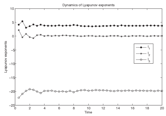
Figure 2. Plot of Lyapunov exponents

2.5. Numerical Simulations

Time series analysis of the system (4)-(6) according to $x(t),y(t),z(t)$ axes are listed in the Figure 3. For the solutions of the system the Runge-Kutta method was employed.

(a)

(b)

(c)

Figure 3. Waveforms of $x(t)$, $y(t)$, $z(t)$ respectively

Obviously the time series show that the functions $x(t)$, $y(t)$, and $z(t)$ are not periodic, indicating that the system is chaotic.

The projections of the system (4)-(6), on the various axes is given in the Figure 4.

(a)

(b)

(c)

Figure 4. Projection of System (4)-(6) on the x-y plane, x-z plane, y-z plane respectively

The chaotic attractors are displayed in the Figure 4. It appears that the new attractor exhibits an interesting complex chaotic dynamics behavior.

3. Geometric and Bigeometric Sense of New System

As an application of the dynamical systems, the newly formed chaotic system can also be written in the sense of Geometric and the Bigeometric calculus.

3.1. Geometric and the Bigeometric Chaotic Systems

The Geometric Chaotic system corresponding to system (4)-(6), can be written as

(16) $$\frac{d^{*}x}{dt} =e^{\frac{\sigma(yz-x)}{x}}$$

$$\frac{d^{*}y}{dt} =e^{\frac{\rho x-xz}{y}}$$

$$\frac{d^{*}z}{dt} =e^{\frac{(xy)^{2}-\beta z}{z}}$$

On the other hand, the Bigeometric Chaotic system corresponding to system (4)-(6) will be

(17) $$\frac{d^{\pi}x}{dt} =e^{\frac{t(\sigma(yz-x))}{x}}$$

$$\frac{d^{\pi}y}{dt} =e^{\frac{t(\rho x-xz)}{y}}$$

$$\frac{d^{\pi}z}{dt} =e^{\frac{t((xy)^{2}-\beta z)}{z}}$$

In order to solve the system (16), one can use the Geometric Runge-Kutta method defined in [22], while the system (17) can be solved by using the Bigeometric Runge-Kutta method which was defined in [23]. By choosing the same values for the parameters, such as $\sigma=12$, $\rho=8$ with varying $\beta$ and the initial values as $(0,0,0)$, we can see that the solutions of the Geometric chaotic system (16) and the Bigeometric chaotic system (17) will be similar to the ones that we get from the solutions of the chaotic system (4)-(6). The following figure shows the chaotic behaviour of the Geometric and the Bigeometric dynamic systems when the parameters are chosen as $\sigma=12$, $\rho=8$ and $\beta=4$.

Figure 5. $\beta=4$

4. Conclusion

The proposed modified quadratic Lorenz attractor was analysed theoretically and numerically showing that this system is chaotic. Following the standardized analysis method for chaotic systems, we determined first the equilibria points and the eigenvalues of the Jacobian matrix at these equilibria points to get a first indication about the stability of the proposed system. As the eigenvalues are either non-positive real numbers, or complex numbers with positive real parts, we can conclude that this system is not stable at the equilibria points. Moreover, we could identify that the proposed system has a rotational symmetry about the $z$-axis, and shows dissipative behaviour contracting the volume element $V_{0}$ to $V_{0}e^{-16}$. The Lyapunov exponents yield to $l_{1}=5.4162$ , $l_{2}=2.1912$ and $l_{3}=-19.2269$, showing the chaotic nature of the system. The fractional dimension of the system $D_{L}=2.3957$ has also been given. Overall, the analysis shows that this is a new chaotic system with two scrolls.

5. References

References

- Aniszewska [2007] Dorota Aniszewska. Multiplicative runge–kutta methods. Nonlinear Dynamics, 50(1):265–272, 2007.
- Arnold [1989] Vladimir Igorevich Arnold. Mathematical methods of classical mechanics, volume 60. Springer Science & Business Media, 1989.
- Birkhoff [1927] George D Birkhoff. On the periodic motions of dynamical systems. Acta Mathematica, 50(1):359–379, 1927.
- Cartwright and Littlewood [1947] ML Cartwright and JE Littlewood. On non-linear differential equations of the second order: Ii. the equation ̵̈y+kf(y,̇y+g(y,k)=p(t)=p_1(t)+kp_2(t);k¿0,f(y)underline¿1. Annals of Mathematics, pages 472–494, 1947.
- Chen and Ueta [1999] Guanrong Chen and Tetsushi Ueta. Yet another chaotic attractor. International Journal of Bifurcation and Chaos, 9(07):1465–1466, 1999.
- Chlouverakis and Sprott [2005] Konstantinos E Chlouverakis and JC Sprott. A comparison of correlation and lyapunov dimensions. Physica D: Nonlinear Phenomena, 200(1):156–164, 2005.
- Cuomo and Oppenheim [1993] Kevin M Cuomo and Alan V Oppenheim. Circuit implementation of synchronized chaos with applications to communications. Physical review letters, 71(1):65–68, 1993.
- Fatou [1917] Pierre Fatou. Sur les substitutions rationnelles. Comp. Rend. heb. S. Acad, Sci, 164:806–808, 1917.
- Hahn and Baartz [1967] Wolfgang Hahn and Arne P Baartz. Stability of motion, volume 422. Springer, 1967.
- Julia [1918] Gaston Julia. Mémoire sur l’itération des fonctions rationnelles. Journal de mathématiques pures et appliquées, pages 47–246, 1918.
- Kolmogorov [1979] A. A. N. Kolmogorov. Preservation of conditionally periodic movements with small change in the Hamilton function. In G. Casati and J. Ford, editors, Stochastic Behavior in Classical and Quantum Hamiltonian Systems, volume 93 of Lecture Notes in Physics, Berlin Springer Verlag, pages 51–56, 1979. doi: 10.1007/BFb0021737.
- Kolmogorov [1991] A. N. Kolmogorov. Dissipation of Energy in the Locally Isotropic Turbulence. Royal Society of London Proceedings Series A, 434:15–17, July 1991. doi: 10.1098/rspa.1991.0076.
- Kolmogorov [1941] Andrey Nikolaevich Kolmogorov. The local structure of turbulence in incompressible viscous fluid for very large reynolds numbers. In Dokl. Akad. Nauk SSSR, volume 30, pages 299–303, 1941.
- Kyrtsou and Labys [2006] Catherine Kyrtsou and Walter C Labys. Evidence for chaotic dependence between us inflation and commodity prices. Journal of Macroeconomics, 28(1):256–266, 2006.
- Kyrtsou and Vorlow [2005] Catherine Kyrtsou and Constantinos E Vorlow. Complex dynamics in macroeconomics: A novel approach. In New Trends in Macroeconomics, pages 223–238. Springer, 2005.
- Lorenz [1963] Edward N Lorenz. Deterministic nonperiodic flow. Journal of the atmospheric sciences, 20(2):130–141, 1963.
- Lü and Chen [2002] Jinhu Lü and Guanrong Chen. A new chaotic attractor coined. International Journal of Bifurcation and chaos, 12(03):659–661, 2002.
- Lu [2006] Jun Guo Lu. Chaotic dynamics of the fractional-order lü system and its synchronization. Physics Letters A, 354(4):305–311, 2006.
- Pehlivan and UYAROĞLU [2010] Ihsan Pehlivan and YILMAZ UYAROĞLU. A new chaotic attractor from general lorenz system family and its electronic experimental implementation. Turkish Journal of Electrical Engineering & Computer Sciences, 18(2):171–184, 2010.
- Peters [1994] Edgar E Peters. Fractal market analysis: applying chaos theory to investment and economics, volume 24. John Wiley & Sons, 1994.
- Poincaré [1890] Henri Poincaré. Sur le problème des trois corps et les équations de la dynamique. Acta mathematica, 13(1):A3–A270, 1890.
- Riza and Aktöre [2015] M. Riza and H. Aktöre. The Runge-Kutta Method in Geometric Multiplicative Calculus. ArXiv e-prints 1311.6108v2, January 2015.
- Riza and Eminağa [2014] Mustafa Riza and Buğçe Eminağa. Bigeometric calculus - a modelling tool. arXiv preprint arXiv:1402.2877, 02 2014. URL http://arxiv.org/abs/1402.2877.
- Rössler [1976] Otto E Rössler. An equation for continuous chaos. Physics Letters A, 57(5):397–398, 1976.
- Rössler [1981] Otto E Rössler. Chaos and chemistry. In Nonlinear Phenomena in Chemical Dynamics, pages 79–87. Springer, 1981.
- Shaw [1981] Robert Shaw. Strange attractors, chaotic behavior and information flow. Z. Naturforsch., 36:80–112, 1981.
- Smale [1960] Stephen Smale. Morse inequalities for a dynamical system. Bulletin of the American Mathematical Society, 66(1):43–49, 1960.
- Smale [1961] Stephen Smale. On gradient dynamical systems. Annals of Mathematics, pages 199–206, 1961.
- Tél et al. [2005] Tamás Tél, Alessandro de Moura, Celso Grebogi, and György Károlyi. Chemical and biollogical activity in open flows: A dynamical system approach. Physics reports, 413(2):91–196, 2005.
- Yang et al. [2010] Qigui Yang, Zhouchao Wei, and Guanrong Chen. An unusual 3d autonomous quadratic chaotic system with two stable node-foci. International Journal of Bifurcation and Chaos, 20(04):1061–1083, 2010.
- Yu et al. [2006] Simin Yu, Jinhu Lü, Wallace KS Tang, and Guanrong Chen. A general multiscroll lorenz system family and its realization via digital signal processors. Chaos: An Interdisciplinary Journal of Nonlinear Science, 16(3):033126, 2006.
- Zhao [2013] Xiao-Qiang Zhao. Dynamical systems in population biology. Springer Science & Business Media, 2013.