Binary Neutron Stars with Arbitrary Spins in Numerical Relativity

Abstract

We present a code to construct initial data for binary neutron star systems in which the stars are rotating. Our code, based on a formalism developed by Tichy, allows for arbitrary rotation axes of the neutron stars and is able to achieve rotation rates near rotational breakup. We compute the neutron star angular momentum through quasi-local angular momentum integrals. When constructing irrotational binary neutron stars, we find a very small residual dimensionless spin of $\sim 2\times 10^{-4}$. Evolutions of rotating neutron star binaries show that the magnitude of the stars’ angular momentum is conserved, and that the spin- and orbit-precession of the stars is well described by post-Newtonian approximation. We demonstrate that orbital eccentricity of the binary neutron stars can be controlled to $\sim 0.1\%$. The neutron stars show quasi-normal mode oscillations at an amplitude which increases with the rotation rate of the stars.

I Introduction

Several known binary neutron star (BNS) systems will merge within a Hubble time due to inspiral driven by gravitational radiation Lorimer (2008), most notably the Hulse-Taylor pulsar Hulse and Taylor (1975). Therefore, binary neutron stars constitute one of the prime targets for upcoming gravitational wave detectors like Advanced LIGO Harry (2010); Aasi et al. (2015) and Advanced Virgo The Virgo Collaboration (2010); Acernese et al. (2015). The neutron stars in known binary pulsars have fairly long rotation periods Lorimer (2008). The system J0737-3039 Lyne et al. (2004) contains the fastest known spinning neutron star in a binary with a rotation period of 22.7ms. This system will merge within $\sim 10^{8}$ years through gravitational wave driven inspiral. Globular clusters contain a significant fraction of all known milli-second pulsars Lorimer (2008), which through dynamic interactions, may form binaries Lee et al. (2010); Benacquista and Downing (2013). Gravitational wave driven inspiral reduces Peters and Mathews (1963); Peters (1964) the initially high eccentricity of dynamical capture binaries. Given the presence of milli-second pulsars in globular clusters, dynamically formed BNS may contain very rapidly spinning neutron stars with essentially arbitrary spin orientations. Presence of spin in BNS systems does influence the evolution of the binary. For instance, in order to avoid a loss in sensitivity in GW searches, one needs to account for the NS spin Brown et al. (2012). Furthermore, early BNS simulations Shibata and Uryu (2000) of irrotational and corotational BNS systems found that the spin of corotating BNS noticeably increased the size of accretion discs occurring during the merger of the two NS. The properties of accretion discs and unbound ejecta are intimately linked to electromagnetic and neutrino emission from merging compact object binaries Metzger and Berger (2012). Understanding the behavior of rotating BNS systems is therefore important to quantify the expected observational signatures from such systems. These considerations motivated a recent interest in the numerical modeling of rotating binary neutron star systems during their last orbits and coalescence. Baumgarte and Shapiro Baumgarte and Shapiro (2009), Tichy Tichy (2011), and East et al East et al. (2012) presented formalisms for constructing BNS initial data for spinning neutron stars. Tichy proceeded to construct rotating BNS initial data Tichy (2012); and Ref. Bernuzzi et al. (2014) studies short inspirals and mergers of BNS with rotation rates consistent with known binary neutron stars (i.e. a dimensionless angular momentum of each star $\chi=S/M^{2}\lesssim 0.05$), and rotation axes aligned with the orbital angular momentum. Very recently, Dietrich et al. Dietrich et al. (2015) presented a comprehensive study of BNS, including a simulation of a precessing, merging BNS. East et. al. East et al. (2015) investigate interactions of rotating neutron stars on highly eccentric orbit. Kastaun et al. Kastaun et al. (2013) determine the maximum spin of the black hole remnant formed by the merger of two aligned spin rotating neutron stars. Tsatsin and Marronetti Tsatsin and Marronetti (2013) present initial data and evolutions for non-spinning, spin-aligned and anti-aligned data sets.

Previous studies differ in the type of initial data used: Refs. Baumgarte and Shapiro (2009); Tichy (2011, 2012); Bernuzzi et al. (2014) construct and utilize constraint-satisfying initial data, which also incorporates quasi-equilibrium of the binary system. Refs. East et al. (2012, 2015) construct constraint-satisfying data based on individual TOV stars, without regard of preserving quasi-equilibrium in the resulting binary, but providing greatly enhanced flexibility in the type of configurations that can be studied, e.g. hyperbolic encounters. Refs. Kastaun et al. (2013); Tsatsin and Marronetti (2013), finally, only approximately satisfy the constraint equations. Previous studies also differ in the rigor with which the neutron star angular momentum is measured. Ref. Tichy (2012) merely discusses the neutron stars based on a rotational velocity $\omega^{i}$ entering the initial data formalism (cf. our Eq. (48) below), whereas Refs. Bernuzzi et al. (2014); Kastaun et al. (2013); East et al. (2015) estimate the initial neutron star spin either based on single star models or based on the differences in binary neutron star initial data sets with and without rotation, and thus neglecting the impact of interactions in the binary. All these studies measure the neutron star angular momentum in the initial data. Changes in the neutron star angular momentum that could happen during initial relaxation of the binary or during the subsequent evolution of the binary are not monitored.

In this paper we study the construction of rotating binary neutron star initial data and the evolution through the inspiral phase. We implement the constant rotational velocity (CRV) formalism developed by Tichy Tichy (2012), and construct constraint satisfying BNS initial data sets with a wide variety of spin rates, as well as different spin directions. We apply quasi-local angular momentum techniques developed for black holes to our BNS initial data sets; the quasi-local spin indicates that we are able to construct BNS with dimensionless angular momentum exceeding 0.4. Evolving some of the constructed initial data sets through the inspiral phase, we demonstrate that we can control and reduce orbital eccentricity by an iterative adjustment of initial data parameters controlling orbital frequency and radial velocity of the stars, both for non-precessing (i.e. aligned-spin binaries) and precessing binaries. When monitoring the quasi-angular momentum of the neutron stars during the inspiral, we find that its magnitude is conserved, and the spin-direction precesses in a manner consistent with post-Newtonian predictions.

This paper is organized as follows. Section II describes the initial data formalism and our numerical code to solve for rotating BNS initial data. In Sec. III we use this code to study a range of initial configurations, with a special emphasis on the behavior of the quasi-local spin diagnostic. We evolve rotating BNS in Sec. IV, including a discussion of eccentricity removal, the behavior of the quasi-local spin diagnostics, and a comparison of the precession dynamics to post-Newtonian theory. A discussion concludes the paper in Sec. V. In this paper, we work in units where $G=c=M_{\odot}=1$.

II Methodology

II.1 Formalism for irrotational binaries

To start, we will review a formalism commonly used for the construction of initial data for system of irrotational binary neutron stars. We will then discuss how to build upon this formalism to construct initial data for neutron stars with arbitrary spins.

We begin with the 3+1 decomposition of the space-time metric (see Gourgoulhon (2007) for a review),

$$ds^{2}=-\alpha^{2}dt^{2}+\gamma_{ij}\left(dx^{i}+\beta^{i}dt\right)\left(dx^{j}+\beta^{j}dt\right).$$ (1)

Here, $\alpha$ is the lapse function, $\beta^{i}$ is the shift vector and $\gamma_{ij}$ is the 3-metric induced on a hypersurface $\Sigma(t)$ of constant coordinate time $t$. In this decomposition, the unit normal vector $n^{\mu}$ to $\Sigma(t)$ and the tangent vector $t^{\mu}$ to the coordinate line $t$ are related by

$$t^{\mu}=\alpha n^{\mu}+\beta^{\mu},$$ (2)

with $n_{\mu}=(-\alpha,0,0,0)$ and $\beta^{\mu}=(0,\beta^{i})$. The extrinsic curvature of $\Sigma(t)$ is the symmetric tensor defined as

$$K_{\mu\nu}=-\nabla_{\nu}n_{\mu}-n_{\nu}\gamma^{\lambda}_{\phantom{\lambda}\mu}\nabla_{\lambda}(\ln\alpha)=-\frac{1}{2}\mathcal{L}_{n}\gamma_{\mu\nu},$$ (3)

where $\gamma_{\mu\nu}=g_{\mu\nu}+n_{\mu}n_{\nu}$ is the extension of the 3-metric $\gamma_{ij}$ to the 4-dimensional spacetime, and $g_{\mu\nu}$ is the 4-metric of that spacetime. By construction, $K^{\mu\nu}n_{\mu}=0$ and we can restrict $K^{\mu\nu}$ to the 3-dimensional tensor $K^{ij}$ defined on $\Sigma\times\Sigma$. The extrinsic curvature $K^{ij}$ is then divided into its trace $K$ and trace-free part $A^{ij}$:

$$K^{ij}=A^{ij}+\frac{1}{3}\gamma^{ij}K.$$ (4)

We treat the matter as a perfect fluid with stress-energy tensor

$$T_{\mu\nu}=\left(\rho+P\right)u_{\mu}u_{\nu}+Pg_{\mu\nu},$$ (5)

where $\rho=\rho_{0}(1+\epsilon)$ is the energy density, $\rho_{0}$ the baryon density, $\epsilon$ the specific internal energy, $P$ the pressure, and $u_{\mu}$ the fluid’s 4-velocity. For the initial value problem, it is often convenient to consider the following projections of the stress tensor:

$$E = T^{\mu\nu}n_{\mu}n_{\nu},$$ (6)

$$S = \gamma^{ij}\gamma_{i\mu}\gamma_{j\nu}T^{\mu\nu},$$ (7)

$$J^{i} = -\gamma^{i}_{\phantom{i}\mu}T^{\mu\nu}n_{\nu}.$$ (8)

We then further decompose the metric according to the conformal transformation

$$\gamma_{ij}=\Psi^{4}\tilde{\gamma}_{ij}.$$ (9)

Other quantities have the following conformal transformations:

$$E = \Psi^{-6}\tilde{E},$$ (10)

$$S = \Psi^{-6}\tilde{S},$$ (11)

$$J^{i} = \Psi^{-6}\tilde{J}^{i},$$ (12)

$$A^{ij} = \Psi^{-10}\tilde{A}^{ij},$$ (13)

$$\alpha = \Psi^{6}\tilde{\alpha}.$$ (14)

$\tilde{A}^{ij}$ is related to the shift and the time derivative of the conformal metric, $\tilde{u}_{ij}=\partial_{t}\tilde{\gamma}_{ij}$ by

$$\tilde{A}^{ij}=\frac{1}{2\tilde{\alpha}}\left[\left(\tilde{\mathbb{L}}\beta\right)^{ij}-\tilde{u}^{ij}\right],$$ (15)

where $\tilde{\mathbb{L}}$ is the conformal longitudinal operator whose action on a vector $V^{i}$ is

$$\left(\tilde{\mathbb{L}}V\right)^{ij}=\tilde{\nabla}^{i}V^{j}+\tilde{\nabla}^{j}V^{i}-\frac{2}{3}\tilde{\gamma}^{ij}\tilde{\nabla}_{k}V^{k},$$ (16)

and $\tilde{\nabla}$ is the covariant derivative defined with respect to the conformal 3-metric $\tilde{\gamma}_{ij}$.

In the 3+1 formalism, the Einstein equations are decomposed into a set of evolution equations for the metric variables as a function of $t$, and a set of constraint equations on each hypersurface $\Sigma(t)$. The initial data problem consists in providing quantities $g_{\mu\nu}(t_{0})$ and $K_{\mu\nu}(t_{0})$ which satisfy the constraints on $\Sigma(t_{0})$ and represent initial conditions with the desired physical properties (e.g. masses and spins of the objects, initial orbital frequency, eccentricity, etc.).We solve the constraint equations using the Extended Conformal Thin Sandwich (XCTS) formalism York (1999), in which the constraints take the form of five nonlinear coupled elliptic equations. The XCTS equations can be written as

$$2\tilde{\alpha}\bigg{[}\tilde{\nabla}_{j}\left(\frac{1}{2\tilde{\alpha}}\big{(}\tilde{L}\beta\big{)}^{ij}\right)-\tilde{\nabla}_{j}\left(\frac{1}{2\tilde{\alpha}}\tilde{u}^{ij}\right)$$

$$-\frac{2}{3}\Psi^{6}\tilde{\nabla}^{i}K-8\pi\Psi^{4}\tilde{J}^{i}\bigg{]} = 0,$$ (17)

$$\tilde{\nabla}^{2}\Psi-\frac{1}{8}\Psi\tilde{R}-\frac{1}{12}\Psi^{5}K^{2}\qquad\quad$$

$$+\frac{1}{8}\Psi^{-7}\tilde{A}_{ij}\tilde{A}^{ij}+2\pi\Psi^{-1}\tilde{E} = 0,$$ (18)

$$\tilde{\nabla}^{2}\left(\tilde{\alpha}\Psi^{7}\right)-\left(\tilde{\alpha}\Psi^{7}\right)\bigg{[}\frac{1}{8}\tilde{R}+\frac{5}{12}\Psi^{4}K^{2}+\frac{7}{8}\Psi^{-8}\tilde{A}_{ij}\tilde{A}^{ij}$$

$$+2\pi\Psi^{-2}\big{(}\tilde{E}+2\tilde{S}\big{)}\bigg{]}=-\Psi^{5}\left(\partial_{t}K-\beta^{k}\partial_{k}K\right).$$ (19)

We solve these equations for the conformal factor $\Psi$, the densitized lapse $\tilde{\alpha}\Psi^{7}$ and the shift $\beta^{i}$. $\tilde{E}$, $\tilde{S}$ and $\tilde{J}^{i}$ determine the matter content of the slice. The variables $\tilde{\gamma}_{ij}$, $\tilde{u}_{ij}=\partial_{t}\tilde{\gamma}_{ij}$, $K$ and $\partial_{t}K$ are freely chosen.

If we work in a coordinate system corotating with the binary, $\tilde{u}_{ij}=0$ and $\partial_{t}K=0$ are natural choices for a quasi-equilibrium configuration. Following earlier work Taniguchi et al. (2007, 2006); Foucart et al. (2008), we also choose to use maximal slicing, $K=0$, and a conformally flat metric, $\tilde{\gamma}_{ij}=\delta_{ij}$. Maximal slicing is a gauge choice that determines the location of the initial data hypersurface in the embedding space time. Conformal flatness is used for computational convenience; rotating black holes are known to be not conformally flat Garat and Price (2000), and so this simplifying assumption should be revisited in the future.

In addition to solving these equations for the metric variables, we must impose some restrictions on the matter. In particular, the stars should be in a state of approximate hydrostatic equilibrium in the comoving frame. This involves solving the Euler equation and the continuity equation. For an irrotational binary, the first integral of the Euler equation leads to the condition

$$h\alpha\frac{\gamma}{\gamma_{0}}=C,$$ (20)

where $C$ is a constant, hereafter referred to as the Euler constant, the enthalpy $h$ is defined as

$$h=1+\epsilon+\frac{P}{\rho_{0}},$$ (21)

and we have introduced

$$\gamma = \gamma_{n}\gamma_{0}\left(1-\gamma_{ij}U^{i}U^{j}_{0}\right),$$ (22)

$$\gamma_{0} = \left(1-\gamma_{ij}U^{i}_{0}U^{j}_{0}\right)^{-1/2},$$ (23)

$$\gamma_{n} = \left(1-\gamma_{ij}U^{i}U^{j}\right)^{-1/2},$$ (24)

$$U^{i}_{0} = \frac{\beta^{i}}{\alpha}.$$ (25)

The 3-velocity $U^{i}$ is defined by

$$u^{\mu} = \gamma_{n}(n^{\mu}+U^{\mu}),$$ (26)

$$U^{\mu}n_{\mu} = 0.$$ (27)

The choice of $U^{i}$, which is unconstrained in this formalism, is an important component is determining the initial conditions in the neutron star. For irrotational binaries (non-spinning neutron stars), there exists a potential $\phi$ such that

$$U^{i}=\frac{\Psi^{-4}\tilde{\gamma}^{ij}}{h\gamma_{n}}\partial_{j}\phi.$$ (28)

The continuity equation can then be written as a second-order elliptic equation for $\phi$:

$$\frac{\rho_{0}}{h}\nabla^{\mu}\nabla_{\mu}\phi+\left(\nabla^{\mu}\phi\right)\nabla_{\mu}\frac{\rho_{0}}{h}=0.$$ (29)

Under the assumption of the existence of an approximate helicoidal Killing vector $\xi$ Teukolsky (1998); Shibata (1998), this equation becomes

$$\rho_{0}\,\bigg{\{}\!\! -\tilde{\gamma}^{ij}\partial_{i}\partial_{j}\phi+\frac{h\beta^{i}\Psi^{4}}{\alpha}\partial_{i}\gamma_{n}+hK\gamma_{n}\Psi^{4}$$

$$\quad+\left[\tilde{\gamma}^{ij}\tilde{\Gamma}^{k}_{ij}+\gamma^{ik}\partial_{i}\left(\ln\frac{h}{\alpha\Psi^{2}}\right)\right]\partial_{k}\phi\bigg{\}}$$

$$=\tilde{\gamma}^{ij}\partial_{i}\phi\partial_{j}\rho_{0}-\frac{h\gamma_{n}\beta^{i}\Psi^{4}}{\alpha}\partial_{i}\rho_{0}.$$ (30)

Another simple choice for $U^{i}$ is to enforce corotation of the star, i.e. $U^{i}=U^{i}_{0}$. This would be the case if neutron star binaries were tidally locked. However, viscous forces in neutron stars are expected to be insufficient to impose tidal locking Bildsten and Cutler (1992), and the neutron star spins probably remain close to their value at large orbital separations.

Once we have obtained $h$ from the metric and $U^{i}$, the other hydrodynamical variables can be recovered if we close the system by the choice of an equation of state for cold neutron star matter in $\beta$-equilibrium, $P=P(\rho_{0})$ and $\epsilon=\epsilon(\rho_{0})$. Throughout this work, we use a polytropic equation of state, $P=\kappa\rho_{0}^{\Gamma}$, with $\Gamma=2$. The internal energy, $\epsilon\rho_{0}$, satisfies

$$\epsilon\rho_{0}=\frac{P}{\Gamma-1}.$$ (31)

The boundary conditions of our system of equations are quite simple. At the outer boundary of the computational domain (which we approximate as “infinity” and is in practice $10^{10}M_{\odot}$), we require the metric to be Minkowski in the inertial frame, and so in the corotating frame we have

$${\bm{\beta}} = {\bm{\Omega}}_{0}\times{\bm{r}}+\dot{a}_{0}{\bm{r}},$$ (32)

$$\alpha = 1,$$ (33)

$$\Psi = 1,$$ (34)

with ${\bm{\Omega}}_{0}$ the initial orbital frequency of the binary and $\dot{a}_{0}$ the initial inspiral rate of the binary. We choose ${\bm{\Omega}}_{0}=(0,0,\Omega_{0})$, with $\Omega_{0}$ and $\dot{a}_{0}$ as freely specifiable variables that determine the initial eccentricity of the binary.

At the surface of each star, the boundary condition can be easily inferred from the $\rho_{0}=0$ limit of equation (30):

$$\tilde{\gamma}^{ij}\partial_{i}\phi\partial_{j}\rho_{0}=\frac{h\gamma_{n}\beta^{i}\Psi^{4}}{\alpha}\partial_{i}\rho_{0}.$$ (35)

Finally, we discuss how a first guess for the orbital angular velocity $\Omega_{0}$ can be obtained for a non-spinning system. The force balance equation at the centre of the NS is

$$\nabla\ln{h}=0.$$ (36)

Neglecting any infall velocity, this condition guarantees that the binary is in a circular orbit. This is only an approximation as there is really some infall velocity, but this still leads to low eccentricity binaries with $e\sim 0.01$. From the integrated Euler equation, we can write this condition as

$$\nabla\ln{h}=\nabla\left(\ln{\frac{\gamma_{0}}{\alpha\gamma}}\right)=0,$$ (37)

or, by using the definitions of $\gamma_{0}$, and $\gamma$,

$$\nabla\ln\left(\alpha^{2}-\gamma_{ij}\beta^{i}\beta^{j}\right)=-2\nabla\ln{\gamma}.$$ (38)

If we decompose $\beta^{i}$ in its inertial component $\beta^{i}_{0}$ and its comoving component according to

$${\bm{\beta}}={\bm{\beta}}_{0}+{\bm{\Omega}}_{0}\times{\bm{r}}+\dot{a}_{0}{\bm{r}},$$ (39)

this can be written as a quadratic equation for the orbital angular velocity $\Omega_{0}$ (neglecting the dependence of $\gamma$ on the orbital angular velocity $\Omega_{0}$). In practice, we solve for $\Omega_{0}$ by projecting Eq. (38) along the line connecting the center of the two stars.

The exact iterative procedure followed to solve in a consistent manner the constraint equations, the elliptic equations for $\phi$, and the algebraic equations for $h$ (including on-the-fly computation of $\Omega_{0}$ and of the constant in the first integral of Euler equation) is detailed in Section II.4.

Once a quasi-equilibrium solution has been obtained by this method, lower eccentricity systems can be generated by modifying $\Omega_{0}$ and $\dot{a}_{0}$, following the methods developed by Pfeiffer et al. Pfeiffer et al. (2007).

II.2 Formalism for Spinning Binaries

We will now discuss how to alter the formalism discussed above to incorporate spinning BNS. Although several formalisms have been introduced in the past Marronetti and Shapiro (2003)Baumgarte and Shapiro (2009), we will follow the work of Tichy (2011)Tichy (2011). A first obvious difference is that we can no longer write the velocity solely in terms of the gradient of a potential. Following Tichy, we break the velocity up into an irrotational part, and a new rotational part $W$:

$$U^{i}=\frac{\Psi^{-4}\tilde{\gamma}^{ij}}{h\gamma_{n}}\left(\partial_{j}\phi+W_{j}\right),$$ (40)

where it is natural, although not required, for $W$ to be divergenceless.

Following the assumptions stated in TichyTichy (2011), the continuity equation becomes

$$\rho_{0}\,\bigg{\{}\!\! -\tilde{\gamma}^{ij}\partial_{i}\big{(}\partial_{j}\phi+W_{j}\big{)}+\frac{h\beta^{i}\Psi^{4}}{\alpha}\partial_{i}\gamma_{n}+hK\gamma_{n}\Psi^{4}$$

$$\qquad+\Big{[}\tilde{\gamma}^{ij}\tilde{\Gamma}^{k}_{ij}+\gamma^{ik}\partial_{i}\big{(}\ln\frac{h}{\alpha\Psi^{2}}\big{)}\Big{]}\big{(}\partial_{k}\phi+W_{k}\big{)}\bigg{\}}$$

$$=\tilde{\gamma}^{ij}\big{(}\partial_{i}\phi+W_{i}\big{)}\partial_{j}\rho_{0}-\frac{h\gamma_{n}\beta^{i}\Psi^{4}}{\alpha}\partial_{i}\rho_{0}.$$ (41)

Eq. 41 then is the same as in the irrotational case, cf. Eq. 30, under the replacement $\partial_{i}\phi\rightarrow\partial_{i}\phi+W_{i}$.

Taking the limit $\rho_{0}\to 0$ in Eq. (41) yields the boundary condition at the surface of each star:

$$\tilde{\gamma}^{ij}\left(\partial_{i}\phi+W_{i}\right)\partial_{j}\rho_{0}=\frac{h\gamma_{n}\beta^{i}\Psi^{4}}{\alpha}\partial_{i}\rho_{0}.$$ (42)

The solution of the Euler equation is no longer as simple as it was previously, in Eq. 20. As shown in Tichy(2011)Tichy (2011), the solution is now

$$h=\sqrt{L^{2}-\left(\nabla_{i}\phi+W_{i}\right)\left(\nabla^{i}\phi+W^{i}\right)},$$ (43)

where

$$L^{2}=\frac{b+\sqrt{b^{2}-4\alpha^{4}\left(\left(\nabla_{i}\phi+W_{i}\right)W^{i}\right)^{2}}}{2\alpha^{2}},$$ (44)

and

$$b=\left(\beta^{i}\nabla_{i}\phi+C\right)^{2}+2\alpha^{2}\left(\nabla_{i}\phi+w_{i}\right)w^{i}.$$ (45)

Finally, the method discussed previously of modifying the star’s angular velocity is now no longer as simple. The equation is modified to

$$\nabla\ln\left(\alpha^{2}-\gamma_{ij}\beta^{i}\beta^{j}\right)=-2\nabla\ln\Gamma,$$ (46)

where

$$\Gamma=\frac{\gamma_{n}\left(1-\left(\beta^{i}+\frac{W^{i}\alpha}{h\gamma_{n}}\right)\frac{\nabla_{i}\phi}{\alpha h\gamma_{n}}-\frac{W_{i}W^{i}}{\alpha^{2}\gamma_{n}^{2}}\right)}{\sqrt{1-\left(\frac{\beta^{i}}{\alpha}+\frac{W^{i}}{h\gamma_{n}}\right)\left(\frac{\beta_{i}}{\alpha}+\frac{W_{i}}{h\gamma_{n}}\right)}}.$$ (47)

Let us now discuss the choice of the spin term, $W$. This term is, in principle, freely chosen, and so we must choose it so as to best represent the physical situation at hand - namely a uniform rotation with constant angular velocity. As suggested by Tichy(2011)Tichy (2011) and Tichy(2012)Tichy (2012), a reasonable choice for $W$ is

$$W^{i}=\epsilon^{ijk}\omega^{j}r^{k},$$ (48)

where $r^{k}$ is the position vector centered at the star’s centre, $\omega^{j}$ represents an angular velocity vector and $\epsilon^{ijk}=\left\{\pm 1,0\right\}$. This leads to a vector field $W^{i}$ with vanishing divergence in the conformal metric $\tilde{g}_{ij}=\delta_{ij}$. Alternatively, one might prefer a vector field $V^{i}$ with vanishing divergence with respect to the physical metric $g_{ij}=\Psi^{4}\delta_{ij}$. Owing to the conformal transformation properties of the divergence operator, $V^{i}$ is given by

$$V^{i}=\Psi^{-6}W^{i}.$$ (49)

Here, we generally use $W^{i}$ as we have found that it leads to initial data which is closer to being in equilibrium, as we will further discuss in section IV.5.

II.3 Solving the elliptic equations

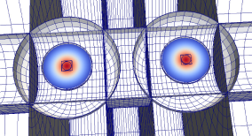
Figure 1: Visualization in the x-y plane of the domain decomposition used in our initial data solve. The colour map represents the density of the stars.

In the previous sections, we have reduced the Einstein constraints, Eqs. (17)–(19), as well as the continuity equation (41) to elliptic equations. We solve these equations with the multi-domain pseudo-spectral elliptic solver developed in Pfeiffer et al. (2003), as modified in Foucart et al. (2008) for matter. The computational domain is subdivided into individual subdomains as indicated in Fig. 1: The region near the center of each star is covered by a cube, overlapping the cube is a spherical shell which covers the outer layers of the star. The outer boundary of this shell is deformed to conform to the surface of the star. This places all surfaces at which the solution is not smooth at a subdomain-boundary, which preserves the exponential convergence of spectral methods. Another spherical shell surrounds each star. The inner shells representing the stars and their vicinity are embedded into a structure of five concentric cylinders with three rectangular blocks along the axis connecting the centers of the neutron stars, which overlap the inner spherical shells. The cylinders/blocks in turn are overlapped at large radius by one further spherical shell centered half-way between the two neutron stars. Using an inverse radial mapping, the outer radius of the outer sphere is placed at $10^{10}$.

All variables are decomposed on sets of basis functions depending on the subdomain. The resolution of each domain (i.e., the number of colocation points used) is chosen at the start of the initial data solve, and then subsequently modified several times using an adaptive procedure described below. In this paper, when discussing the total resolution of the domain, we use the notation

$$N^{1/3}=\left(\sum N_{i}\right)^{1/3},$$ (50)

with $N_{i}$ the number of collocation points in the $i$th subdomain. $N^{1/3}$ is thus the cube root of the total number of collaction points in all subdomains.

II.4 Construction of quasi-equilibrium initial data

Construction of initial data for rotating binary neutron stars begins with selecting the physical properties of the system: the equation of state of nuclear matter, the coordinate separation $d$ between the neutron stars, the baryon masses $M^{b}_{1}$ and $M^{b}_{2}$ of the two stars, and their spin vectors ${\bm{\omega}}_{\rm rot,1}$ and ${\bm{\omega}}_{\rm rot,2}$. We also choose the orbital angular frequency $\Omega_{0}$ and the initial inspiral rate $\dot{a}_{0}$.

We generally begin by setting $\Omega_{0}$ to the value for the orbital frequency of a similar irrotational BNS (where $\Omega_{0}$ is determined by the condition of quasi-circularity, Eq. (36)), and $\dot{a}_{0}=0$. These values are then adjusted following the eccentricity reduction method developed by Pfeiffer et al. Pfeiffer et al. (2007). Finally, we use a flat conformal metric, $\tilde{\gamma}_{ij}=\delta_{ij}$, and maximal slicing, $K=0$.

Once all these quantities are fixed, we need to solve self-consistently Eqs. (17)–(19) for the Einstein-constraints, the continuity equation Eq. (41), while simultaneously satisfying conditions to enforce the desired masses of the stars. To do so, we follow an iterative procedure developed originally for black hole-neutron star binaries Foucart et al. (2012).

First, we choose initial guesses for the conformal metric and hydrodynamical variables, using an analytical superposition of two isolated boosted neutron stars.

We then obtain constraint-satisfying initial conditions by applying the following iterative procedure, where $n$ represents the iteration number:

1. Solve the nonlinear XCTS system for the set of metric variables $X=(\beta^{i},\Psi,\alpha\Psi)$, assuming fixed values of the conformal source terms $(\tilde{E},\tilde{S},\tilde{J}^{i}$). The new value $X^{n+1}$ of the metric variables is obtained from their old value $X^{n}$ and, following the relaxation scheme used in Foucart et al. (2008), the solution of the XCTS equations $X^{*}$, using

   $$X^{n+1}=0.3X^{*}+0.7X^{n}.$$ (51)

2. Locate the surface of each star. Representing the surface in polar coordinates centered on each star as $R_{s}^{n}(\theta,\phi)$, we determine $R_{s}^{n}$ to satisfy Foucart et al. (2008) $h(R^{n}_{\rm s}(\theta,\phi),\theta,\phi)=1$. To ensures that the grid-boundary $R_{b}$ converges to the surface of the star, we occassionally modify the numerical grid such that $R_{b}(\theta,\phi)=R^{n}_{s}(\theta,\phi)$. Because this requires a re-initialization of the elliptic solver, the grid is only modified if the stellar surface has settled down, specifically, if

   $$||R^{n}_{\rm s}-R^{n-1}_{\rm s}||<0.1||R^{n}_{\rm s}-R_{b}||.$$ (52)

   Here $||\;.\;||_{2}$ denotes the L2-norm over the surface.

3. For each neutron star, fix the constant in Euler’s first integral so that the baryon mass of the neutron star matches the desired value. We compute the baryon mass as a function of the Euler constant $C$ through

   $$M^{b}_{\rm NS}=\int_{\rm NS}\rho_{0}\Psi^{6}\sqrt{\frac{1}{1-\gamma_{ij}U^{i}U^{j}}}dV,$$ (53)

   and utilize the secant method to drive the mass to the desired value.

4. If desired, adjust the orbital frequency to ensure force-balance at the center of each star by solving Eq. (38). This step is skipped if the orbital frequency is fixed through iterative eccentricity removal, cf. Sec. IV.2.

5. Solve the elliptic equation for the velocity potential $\phi$, and obtain the next guess for $\phi$ using the same relaxation method shown in Eq. 51.

6. Check whether all equations are satisfied to the desired accuracy. If yes, proceed. If no, return to Step 1.

7. Compute the truncation error of the current solution by examining the spectral expansion of the XCTS variables. If this truncation error is undesirably large (typically, if it is $>10^{-9}$), then adjust the number of grid-points in the domain-decomposition and return to Step 1. The adjustment is based on the desired target truncation eror and the measured convergence rate of the solution, cf. Szilágyi (2014).

II.5 Quasi-Local Angular Momentum

The goal of the present paper is to construct spinning BNS initial data and to evolve it. Therefore, we need diagnostics to measure the NS spin, for which we use techniques originally developed for black holes. It is common to discuss the spins of black holes in terms of their dimensionless spin $\chi$,

$$\chi=\frac{S}{M^{2}}.$$ (54)

Here, $S$ is the angular momentum of the black hole, and $M$ is its Christodoulou mass Christodoulou (1970),

$$M^{2}=M_{\rm irr}^{2}+\frac{S^{2}}{4M_{\rm irr}^{2}}.$$ (55)

The irreducible mass $M_{\rm irr}$ is defined based on the area of the hole’s apparent horizon, $M_{\rm irr}=\sqrt{A/16\pi}$. The angular momentum is computed with a surface integral over the apparent horizon Brown and York (1993); Ashtekar et al. (2001); Ashtekar and Krishnan (2003),

$$S=\frac{1}{8\pi}\oint_{\mathcal{H}}\phi^{i}s^{j}K_{ij}dA$$ (56)

where $\mathcal{H}$ is the black hole’s apparent horizon, $s^{j}$ is the outward-pointing unit-normal to $\mathcal{H}$ within the $t={\rm const}$ hypersurface, and $\phi^{i}$ is an azimuthal vector field tangent to $\mathcal{H}$. For spacetimes with axisymmetry, $\phi^{i}$ should be chosen as the rotational Killing vector. In spacetimes without an exact rotational symmetry (e.g. the spacetime of a binary black hole system), one substitutes an approximate Killing vectorCook and Whiting (2007); Lovelace et al. (2008) (AKV). Ref. Lovelace et al. (2008) introduces a minimization principle to define $\phi^{i}$, resulting in an Eigenvalue problem. The three eigenvectors with the lowest eigenvalues (i.e. smallest shear) are taken and used to compute the three components of the spin.

In this paper, we explore the application of quasi-local spin measures to neutron stars. In the absence of apparent horizons $\mathcal{H}$, we need to choose different surface(s) to evaluate Eq. (56).

When constructing initial data, the stellar surface ${\cal S}$ is already determined, so one obvious choice is to integrate over the stellar surface ${\cal S}$. To estimate the ambiguity in quasi-local spin, we furthermore compute $S$ by integrating over coordinate spheres with radii ranging from just outside ${\cal S}$ to larger by about $70\%$. During the evolution, the stars change shape and may even loose mass in tidal tails. Because of these complications, the SpEC evolution code does not track the location of the stellar surface during the evolution, and we shall only monitor $S$ on coordinate spheres.

It is useful to compute a dimensionless spin $\chi$, for instance, for post-Newtonian comparisons. In the absence of a horizon, Eq. (55) is meaningless and we need a different choice for the mass-normalization. Instead, we normalize by each star’s ADM mass, $M_{\rm{ADM}}$, i.e.

$$\chi\equiv\frac{S}{M_{\rm ADM}^{2}}.$$ (57)

The ADM mass is determined by computing the ADM mass of an equilibrium configuration of a single uniformly rotating polytrope in isolation with the same baryon mass and angular momentum as those measured in our binary systems.

The results of the quasi-local spin measures are described in section III.4, which shows that this procedure is numerically robust.

Finally, let us discuss, from an order of magnitude perspective, how the star’s dimensionless spin is related to its more commonly used physical properties. We start with the Newtonian relation $S=2\pi I/P$ between angular momentum $S$, moment of inertia $I$, and rotational period $P$. Writing further $I=f\,R^{2}\,M$, with the dimensionless constant $f$ depending on the stellar density profile, we have

$$\chi \sim\frac{2\pi c}{G}\frac{fR^{2}}{PM}$$

$$=0.48\,\Big{(}\frac{f}{0.33}\Big{)}\Big{(}\frac{R}{12{\rm km}}\Big{)}^{\!2}\Big{(}\frac{M}{1.4M_{\odot}}\Big{)}^{\!-1}\Big{(}\frac{P}{1{\rm ms}}\Big{)}^{\!-1}\!\!.$$ (58)

The factor $c/G$ arises from the transition to geometric units.

This –quite simplistic– estimate shows that millisecond pulsars will have appreciable dimensionless spin $\chi$. Centrifugal breakup of rapidly rotating neutron stars happens at a dimensionless spin in the range $0.65-0.70$ Lo and Lin (2011), with only small dependence on the equation of state and neutron star mass. Ansorg et al Ansorg et al. (2003) studied in detail $\Gamma=2$ polytropes, the equation of state we use here. Ref. Ansorg et al. (2003) finds a dimensionless spin at mass-shedding of $\chi=0.57$.

III Initial Data Results

In this section, we will demonstrate that our code can robustly construct contraint-satisfying initial data for BNS systems with arbitrary spins. As discussed in section II.4, our code consists of a solver that runs for a number of iterations at constant resolution, and then the resolution is increased and this process restarts. We will therefore demonstrate that appropriate quantities converge with both the iterations of iterative scheme described above in Section II.4 and with resolution as the resolution increases.

Name	$M^{b}_{\rm NS}$	${\bm{\omega}}$	$D_{0}$	$\Omega_{0}\times 10^{3}$	$\dot{a}_{0}\times 10^{5}$	$M_{\rm ADM}$	$\vec{\chi}$
S.4z	1.7745	$0.01525\hat{z}$	47.2	5.09594	-1.75	1.648	$0.3765\hat{z}$
S-.05z	1.7745	$-0.00273\hat{z}$	47.2	5.11769	-1.71	1.640	$-0.05018\hat{z}$
S.4x	1.7745	$0.01525\hat{x}$	47.2	5.10064	-2.36	1.648	$0.3714\hat{x}$

Table 1: Parameters for the initial data sets used in testing the initial data solver: $M^{b}_{\rm NS}$ and $\omega^{i}$ are baryon mass and rotational parameter for either neutron star (the same values are used); $D_{0}$, $\Omega_{0}$ and $\dot{a}_{0}$ represent coordinate separation between the centers of the stars, the orbital frequency, and the radial expansion; $\vec{\chi}$ is the dimensionless spin vector computed from the initial data set. In each case we use a polytropic equation of state, $P=\kappa\rho_{0}^{\Gamma}$, with $\Gamma=2$ and $\kappa=123.6$.

III.1 Convergence of the Iterative Procedure

At each step of the iterative procedure, the Euler constant of each star is modified to achieve a desired stellar baryon mass, based on the current matter distribution inside the star. We expect that the Euler constant converges during the iterations at a fixed resolution. Figure 2 shows the behavior of the Euler Constant during iterations at the lowest initial data resolution, R0. We show three runs of interest, one with large aligned spins (S.4z), one with large precessing spin (S.4x), and one with small anti-aligned spins (S-.05z). The properties of these configurations are shown in table 1. In all three cases we see agreement between neighboring iterations at the $10^{-5}-10^{-6}$ level by the end of iterating at this resolution. At the highest resolutions, these differences are down to, typically, the $10^{-9}-10^{-10}$ level. This can be compared to Fig. 3 of Gourgoulhon et al. (2001). Although not shown here, other free quantities converge similarly to the Euler constant.

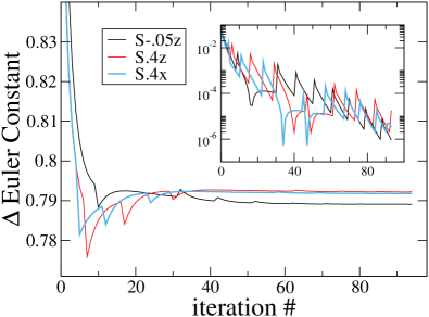
Figure 2: Convergence of the Euler constant during iteration at the lowest resolution R0. The inset shows the difference between values at subsequent iterations.

III.2 Convergence of the Solution

Having established that our iterative procedure converges as intended, we now turn out attention to the convergence of the solution with resolution. To demonstrate it, we will look at the Hamiltonian and momentum constraints, and the differences between measured physical quantities - the ADM energy and ADM angular momentum, and the surface fitting coefficients of the stars. As our initial data representation is fully spectral, we expect that these quantities should converge exponentially with resolution. Note that when we discuss the value of a quantity at a certain resolution, we are referring to the value of that quantity after the final iterative step at that resolution.

Figure 3 shows the convergence of the Hamiltonian constraint and the Momentum constraint for our three runs of interest. These are computed during the last iterative solve at each resolution. The data plotted are computed as

$$H=||\frac{R_{\Psi}}{8\Psi^{5}}||,$$ (59)

$$M=||\frac{R_{\beta}}{2\alpha\Psi^{4}}||.$$ (60)

Here $R_{\Psi}$ and $R_{\beta}$ denote the residuals of Eqs. (18) and (17), respectively, and $||\,.\,||$ represents the root-mean-square value over grid-points of the entire computational grid. This plot demonstrates that our initial data solver converges exponentially with resolution, even for very high spins, which gives confidence that we are indeed correctly solving the Einstein Field Equations.

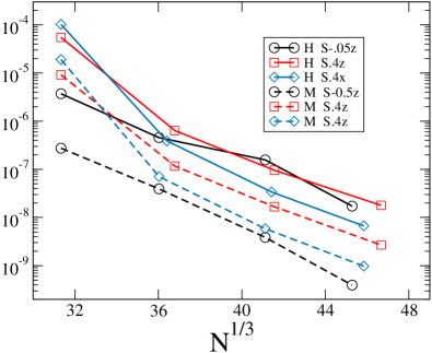
Figure 3: Hamiltonian and Momentum constraints as a function of resolution $N$. We see exponential convergence in all cases.

The surface of the star is represented by a spherical harmonic expansion:

$$R_{s}(\theta,\phi)=\sum^{l_{\rm max},m_{\rm max}}_{l,m}c_{lm}Y_{lm}(\theta,\phi),$$ (61)

where $l_{\rm max}=m_{\rm max}=11$, unless stated otherwise. The stellar surface is located by finding a constant enthalpy surface, cf. Sec. II.4, and the spherical subdomains that cover the star are deformed to conform to $R_{s}(\theta,\phi)$. To establish convergence of the position of the stellar surface we introduce the quantity

$$\Delta c(i)=\frac{1}{l(l+1)}\sqrt{\sum^{l_{\rm max},m_{\rm max}}_{l,m}\left(c_{lm}(i)-c_{lm}(N)\right)^{2}}.$$ (62)

Here $i$ refers to the $i^{\rm th}$ resolution in the initial data, and $N$ refers to the final resolution. Figure 4 plots $\Delta c(i)$ vs. resolution. The surface location converges exponentially to better than $10^{-8}$.

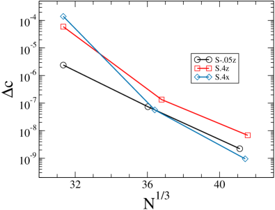
Figure 4: Convergence of the location of the stellar surface. Plotted is $\Delta c$ as defined in Eq.( 62), for three representative configurations.

Finally, we assess the overall convergence of the solution through the global quantities $E_{\rm ADM}$ and $\left|J^{i}_{\rm ADM}\right|$. The surface integrals at infinity in these two quantities are recast using Gauss’ law (cf. Foucart et al. (2008)):

$$E_{\rm ADM} =-\frac{1}{2\pi}\oint_{S_{\infty}}\delta^{i}_{j}\partial_{i}\Psi\,dS_{j}$$

$$=-\frac{1}{2\pi}\oint_{S}\delta^{i}_{j}\partial_{i}\Psi\,dS^{j}+\frac{1}{2\pi}\int_{\mathcal{V}}\delta^{ij}\partial_{i}\partial_{j}\Psi\,dV,$$ (63)

and

$$J^{z}_{\rm ADM} =\frac{1}{8\pi}\oint_{S_{\infty}}\left(xK^{yj}-yK^{xj}\right)dS_{j}$$

$$=\frac{1}{8\pi}\oint_{S}\left(xK_{yi}-yK_{xi}\right)\delta^{ij}\Psi^{2}\,dS_{j}.$$ (64)

Here $\mathcal{V}$ is the volume outside $S$, and the integrals are evaluated in the flat conformal space. To obtain the other components of $J_{\rm ADM}^{i}$, cyclically permute the indices x,y,z. We define the quantities $\Delta E$ and $\Delta J$ as the absolute fractional difference in these quantities between the current resolution and the next highest resolution. These are plotted in figure 5. In general, we find agreement at the $10^{-7}-10^{-8}$ level by the final resolution.

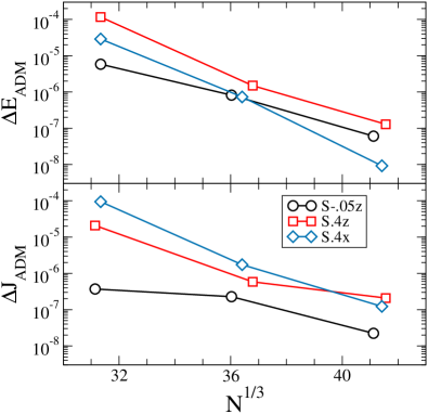
Figure 5: Convergence of ADM-energy and the magnitude of the ADM-angular momentum. Shown are the fractional differences between neighboring resolutions, as a function of the lower resolution.

III.3 Convergence of the quasi-local spin

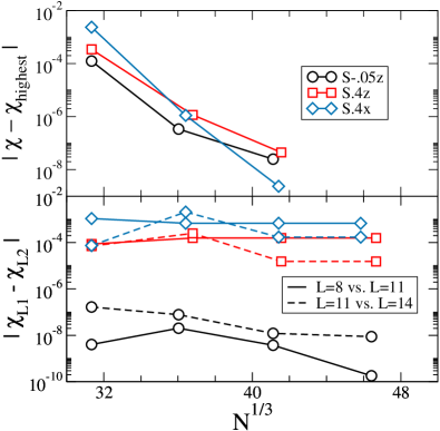
Figure 6: Convergence of the quasi-local spin computation. Top panel: difference of spin computed at resolution $N$ with the spin computed at the highest resolution. Bottom panel: Difference between spins computed at different resolution $L$ of the spin-computation. For S-.5z, we achieve an accuracy of $\sim 10^{-7}$, whereas for S.4z and S.4x, the accuracy is $\sim 10^{-4}$ due to finite $L$.

We now turn to the angular momentum of the neutron stars, as measured with quasi-local angular momentum integrals on the stellar surface. We will discuss dimensionless spins $\chi$, which depend on two distinct numerical resolutions: First, the resolution of the 3-dimensional grid used for solving the initial value equations. This resolution is specified in terms of $N$, the total number of grid-points. Second, the resolution used when solving the eigenvalue problem for approximate Killing vectors on the 2-dimensional surface, as given by $L$, the expansion order in spherical harmonics of the surface-parameterization $r_{S}(\theta,\phi)=\sum_{l=0}^{L}\sum_{m}r_{lm}Y^{lm}(\theta,\phi)$.

Throughout this paper, we use $L=11$. The top panel of Fig. 6 shows convergence of $\chi$ with grid-resolution $N$, at fixed $L=11$. We find near exponential convergence.

The influence of our choice $L=11$ is examined in the lower panel by computing the quasi-local spin at lower resolution $L=8$ and at higher resolution $L=14$. Changing $L$ impacts $\chi$ by $\sim 10^{-8}$ for the low-spin case S-.05z, and by $\sim 10^{-4}$ for the high-spin cases S.4z and S.4x. For the high-spin cases, the spin measurement is convergent with increasing $L$, and the finite value of $L$ dominates the error budget. For the low-spin case, numerical truncation error dominates the error budget and convergence with $L$ is not visible. High NS spin leads to a more distorted stellar surface, and so a fixed $L=11$ yields a spin result of lower accuracy. However, in all cases the the numerical errors of our spin measurements are still neglible for our purposes.

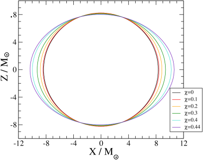
Figure 7: Stellar cross-sections in the X-Z plane for a series of different spins, aligned with the $\hat{z}$ axis, demonstrating that they bulge at the equator in the expected way with increasing spin.

III.4 Quasi-local Spin

As discussed in section II.5, we use a quasi-local spin to define the angular momentum carried by each neutron star. To our knowledge, this is the first application of this method to neutron stars in binaries.

In this section, we explore properties of the rotating BNS initial datasets and the employed quasi-local spin diagnostic.

To explore the spin-dependence of BNS initial data sets, we construct a sequence of equal-mass, equal-spin BNS binaries, with spins parallel to the orbital angular momentum. We fix the initial data parameters $M^{b}_{\rm NS}$, $D_{0}$, $\Omega_{0}$ and $\dot{a}_{0}$ to their values for a configuration that we will also evolve below (specifically, S.4z - Ecc1)

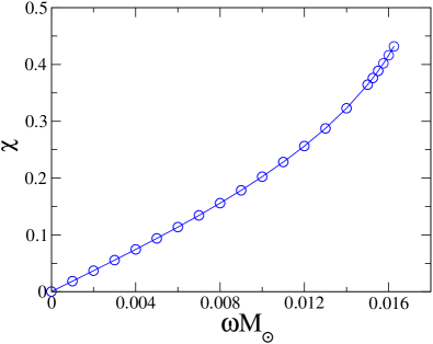
Figure 8: Dimensionless angular momentum $\chi$ as a function of $\Omega$ for a series of spin-aligned initial data sets with the same physical parameters as our runs of interest. We see, as expected, a linear relation between $\chi$ and $\Omega$ at low-spins, which eventually becomes non-linear at higher spins.

Figure 7 shows cross-sections through one of the neutron stars in the xz-plane, i.e. a plane orthogonal to the orbital plane which is intersecting the centers of both stars. With increasing spin, the stars develop an increasing equatorial bulge, an expected consequence of centrifugal forces.

Figure 8 presents the dimensionless spin of either neutron star as a function of $\omega$. $\chi$ increases monotonically with the rotation parameter $\omega$. The spin $\chi$ increases linearly with $\omega$ for small $\omega$. For larger $\omega$, the dependence steepens, as the increasing equatorial radius of the stars increase the moment of inertia Worley et al. (2008).

For $\omega=0.01625M_{\odot}^{-1}$ we achieve $\chi=0.432$, the largest spin we are able to construct. This is reasonably close to the theoretical maximum value for $\Gamma=2$ polytropes, $\chi\sim 0.57$ Ansorg et al. (2003). Above $\omega=0.01625M_{\odot}^{-1}$, the initial data code fails to converge. The steepening of the $\chi$ vs. $\omega$ curve is reminiscent of features related to non-uniqueness of solutions of the extended conformal thin sandwich equations Lovelace et al. (2008); Pfeiffer and York  Jr. (2005); Baumgarte et al. (2007); Walsh (2007), and it is possible that our failure to find solutions originates in an analogous break-down of the uniqueness of solutions of the constraint equations.

While the focus of our investigation lies on rotating NS, we note that for $\omega=0$ our data-sets reduce to the standard formalism for irrotational NS. For $\omega=0$, we find a quasi-local spin of the neutron stars is $\chi=2\times 10^{-4}$. This is the first rigorous measurement of the residual spin of irrotational BNS. Residual spin is, for instance, important for the construction and validation of waveform models for compact object binaries. The analysis in Ref. Boyle et al. (2007) indicates that spins of order $10^{-4}$ lead to a dephasing of about 0.01radians during the last dozen of inspiral orbits. This value is significantly smaller than the phase accuracy obtained by current BNS simulations, and so the residual spin is presently not a limiting factor for studies like Bernuzzi et al. (2015); Baiotti et al. (2011, 2010).

Finally, we demonstrate that the surface on which we compute the quasi-local spin, does not significantly impact the spin we measure: We choose coordinate spheres centered on the neutron star with radius $R$, and compute the quasi-local spin using these surfaces, rather than the stellar surface.

In Fig. 9, we plot the spin measured on various $R=\rm{const}$ surfaces, for three different values of $\omega$, from the same sequences shown in Fig. 8.

The circles denote spins extracted on coordinate spheres. The asterisks indicate the spins computed on the stellar surface. The asterisk is plotted at $R=R_{\rm eq}$, the equatorial radius of the neutron star under consideration. We find good agreement between spins extracted on coordinate spheres and the spin extracted on the stellar surface, as long as $R\geq R_{\rm eq}$. The maximum disagreement is seen in the high spin curve, where the two spins differ by $\sim 10^{-2}$.

For $R<R_{\rm eq}$, the coordinate extraction sphere intersects the outer layers of the neutron star and no longer encompasses the entire matter and angular momentum of the star. Therefore, $\chi(R)$ shows a pronounced decline for $R<R_{\rm eq}$ for each of the three initial-data sets considered in Fig. 9. For $R>R_{\rm eq}$, $\chi(R)$ continues to increase slightly, for instance, for the middle curve, $\chi(R=9)=0.202$ whereas $\chi(R=11)=0.204$.

In summary, Fig. 9 shows that the quasi-local spin extracted on coordinate spheres can serve as a good approximation of the quasi-local spin extracted on the stellar surface (as long as the coordiate sphere is outside the star, of course).

This is important because during evolutions of the binary, we do not track the surface of the star. Instead, we will compute the spin on coordinate spheres, similarly to Fig. 9.

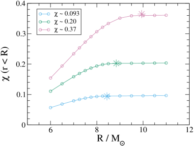
Figure 9: Dimensionless spin $\chi$ measured on coordinate spheres with radius $R$ for three different aligned spin BNS systems. The asterik denotes the spin measured on the (non-spherical) stellar surface. Circles to the right of the asterik represent coordinate spheres entirely outside the neutron star, and circles on the left of the asterik indicate spin measurement surfaces that intersect the star or are entirely located inside the star.

IV Evolution Results

We now evolve the three configurations discussed in Sec. III. As indicated in Table 1, all three configurations are equal-mass binaries, with individual ADM masses $M_{\star}$ (in isolation) of $1.64M_{\odot}$ or $1.648M_{\odot}$ at initial separation of $D=47.2M_{\odot}$, and using a polytropic equation of state with $\Gamma=2.0$ and $\kappa=123.6$. Both stars have equal spins, and the three configurations differ in spin magnitude and spin direction. Configuration S-0.05z has spin-magnitudes $\sim 0.05$ anti-aligned with the orbital angular momentum, and the confiurations S.4z and S.4x have spin magnitudes near 0.4, along the z-axis and x-axis, respectively.

Each configuration is evolved through $\gtrsim 10$ orbits, into the late-inspiral. In this paper we focus on the inspiral of the neutron stars. Table 2 summarizes parameters for these runs.

Name	$k$	$e$	$\vec{\chi}$	$f_{0}(Hz)$	$N_{\rm orb}$	$t_{f}({\rm ms})$
S.4z	0,1,2	$\lesssim 0.001$	$0.381\hat{z}$	$167.7$	$11.8$	$56.0$
S-.05z	0,1,2	$0.0006$	$-0.050\hat{z}$	$165.4$	$12.5$	$56.3$
S.4x	0,1	$\lesssim 0.002$	$0.375\hat{x}$	$164.8$	$9.1$	$45.7$

Table 2: Information about our three evolutions. $k$ indicates the numerical resolutions on which a simulation is performed, $e$ indicates the smallest achieved orbital eccentricity. $\vec{\chi}$ and $f_{0}$ are the dimensionless spins at $t=0$ and the initial orbital frequency. Finally, $N_{\rm orb}$ and $t_{f}$ represent the number of orbits the configuration was evolved for, and the evolution time.

IV.1 Evolution Code

In our evolution code, SpEC Buchman et al. (2012); Lovelace et al. (2012); M. A. Scheel, M. Boyle, T. Chu, L. E. Kidder, K. D. Matthews and H. P. Pfeiffer (2009); Kidder et al. (2000); Lindblom et al. (2006); Scheel et al. (2006); Szilágyi et al. (2009); Lovelace et al. (2011); Hemberger et al. (2013); Ossokine et al. (2013), we use a mixed spectral – finite-difference approach to solving the Einstein Field Equations coupled to general relativistic hydrodynamics equations. The equations for the space-time metric, $g_{\mu\nu}$ are solved on a spectral grid, while the fluid equations are solved on a finite difference grid, using a high-resolution shock-capturing scheme. We use a WENO Jiang and Shu (1996); Liu et al. (1994) reconstruction method to reconstruct primitive variables, and an HLL Riemann solver A. Harten (1983) to compute numerical fluxes at interfaces. Integration is done using a 3rd order Runge-Kutta method with an adaptive stepsize. We interpolate between the hydro and spectral grids at the end of each full time step, interpolating in time to provide data during the Runge-Kutta substeps (see Duez et al. (2008); Foucart et al. (2012, 2013); Muhlberger et al. (2014) for a more detailed description of the method).

Each star is contained in a separate cubical finite difference grid that does not overlap with that of the other star. The sides of the grids are initially $1.25$ times the stars’ diameters. We use grids that contain $97^{3}$, $123^{3}$ and $155^{3}$ points for resolutions $k=0,1,2$, respectively. These resolutions correspond to linear grid-spacing of $340\,\text{m}$, $268\,\text{m}$ and $213\,\text{m}$ respectively for the S.4z case. The precessing evolution S.4x uses similar grid-spacing, whereas the anti-aligned run S-.05z has a slightly smaller grid-spacing because the stars themselves are smaller. The region outside the NS but inside the finite difference grid is filled with a low density atmosphere with $\rho=10^{-13}M_{\odot}^{-2}$. The motion of the NSs is monitored by computing the centroids of the NS mass distributions

$$X^{i}_{\rm CM}=\int{x^{i}u^{0}\rho_{0}\sqrt{-g^{(4)}}d^{3}x}$$ (65)

for each of the grid patches containing a NS.

The grids are rotated and their separation rescaled to keep the centers of the NS at constant grid-coordinates Scheel et al. (2006); Hemberger et al. (2013); Scheel et al. (2015). As the physical separation between the stars decreases, the rescaling of grid-coordinates therefore causes the size of the stars to increase in grid-coordinates. In order to avoid the stellar surfaces expanding beyond the geometric size of the finite difference grid, we monitor the matter flux leaving this grid along the x, y, and z-direction. If the matter flux is too large along a certain axis, we expand the grid in that direction. This procedure allows us to dynamically choose the optimal grid-size that limits matter loss to a small, user-specified level. When changing the size of the hydro grid, the number of grid-points is kept constant, so this process changes the effective resolution during the evolution.

The Einstein field equations are solved on a spectral grid using basis-functions appropriate for the shape of each subdomain. For rectangular blocks, Cheybyshev polynomials are used along each axis; for a spherical shell (i.e. where the center is excised), spherical harmonics in angles, and Chebyshev polynomial in radius are employed; and for an open cylinder (i.e. with the region near the axis excised), Chebyshev polynomials and a Fourier series. For full spheres and filled cylinders, multi-dimensional basis-functions respecting the continuity conditions at the orign/axis are employed Matsushima and Marcus ; Verkley (1997). For more details see Muhlberger et al. (2014).

More specifically, our spectral grid, the central region of each star is covered by a filled sphere located at the center of the star. These have spherical harmonic modes up to $L=12+2k$. The radial basis-functions are one-sided Jacobi polynomials with $7+k$ collocation points. The filled spheres are surrounded by eight other spherical shells with the same radial and angular resolutions. At the start of the evolution, the stellar surface is generally located inside the third shell. The far field region is covered by 20 spherical shells starting at 1.5 times the inital binary separation and going out to 40 times that separation. These shells have angular resolution $L=9+2k$ and radial resolution $6+k$. The region between the innermost shell and the stars is covered by a set of cylindrical shells and filled cylinders.

We use a generalized harmonic evolution system Pretorius (2006, 2005); Lindblom et al. (2006) with coordinates $x^{\mu}$ such that they satisfy a wave equation

$$\nabla^{\nu}\nabla_{\nu}x^{\mu}=H^{\mu},$$ (66)

for some freely-specifiable source function $H^{\mu}$. The initial source function $H^{\mu}_{\rm initial}$ is determined by the intial data, assuming that the time derivatives of the lapse and shift functions initially vanish in the corotating frame. We then transition to a pure harmonic gauge, $H^{\mu}=0$ by using a transition function, i.e.

$$H^{\mu}=e^{-\left(t/\tau\right)^{4}}\;H^{\mu}_{\rm initial}.$$ (67)

The timescale $\tau$ is determined by $\tau=2\sqrt{d^{3}/(2M_{\star})}$. This is slow enough to avoid numerical gauge artifacts in the simulations.

IV.2 Eccentricity Removal

Gravitational wave emission reduces orbital eccentricity rapidly during a GW-driven inspiral Peters and Mathews (1963); Peters (1964). Therefore inspiraling binary neutron stars are expected to have essentially vanishing orbital eccentricity in their late inspiral, unless they recently underwent dynamical interactions. Our goal is to model non-eccentric inspirals. In this subsection we demonstrate that we can indeed control and reduce orbital eccentricty, using the techniques developed for BH-BH binaries Pfeiffer et al. (2007); Boyle et al. (2007); Buonanno et al. (2011) and also applied to BH-NS binaries Foucart et al. (2008).

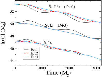
Figure 10: The binary separation as a function of time. Shown are three eccentricity removal iterations (Ecc1,Ecc2,Ecc3) for each of the three configurations studied. The data for S-.05z and S.4z is offset vertically by 6 and 3, respectively, for clarity of plotting.

For fixed binary parameters (masses, spins), and fixed initial separation $D_{0}$, the initial orbit of the binary is determined by two remaining parameters: The initial orbital frequency $\Omega_{0}$, and the initial radial velocity, which we describe through an expansion parameter $\dot{a}_{0}=\dot{r}/r$. These two parameters will encode orbital eccentricty and phase of periastron, and our goal is to determine these parameters to reduce orbital eccentricity. We accomplish this using an iterative procedure first introduced for binary black holes Boyle et al. (2007); Buonanno et al. (2011). An initial data set is evolved for a few orbits, the resulting orbital dynamics are analyzed, and then the initial data parameters $\Omega_{0}$ and $\dot{a}_{0}$ are adjusted.

Name	$\Omega\times 10^{3}$	$\dot{a}_{0}\times 10^{5}$	$e$
S.4z - Ecc1	$5.10538$	$0$	$0.006$
S.4z - Ecc2	$5.09591$	$-1.60$	$\lesssim 0.001$
S.4z - Ecc3	$5.09594$	$-1.75$	$\lesssim 0.001$
S-.05z - Ecc1	$5.10538$	$0$	$0.008$
S-.05z - Ecc2	$5.11561$	$0$	$0.004$
S-.05z - Ecc3	$5.11769$	$-1.71$	$0.0006$
S.4x - Ecc1	$5.10538$	$0$	$0.007$
S.4x - Ecc2	$5.10429$	$-2.27$	$0.004$
S.4x - Ecc3	$5.10064$	$-2.36$	$\lesssim 0.002$

Table 3: Eccentricity removal for the three main runs discussed in this paper. Only initial orbital frequency $\Omega_{0}$ and initial radial expansion factor $\dot{a}_{0}$ are changed between different EccN iterations. Recall that these quantities have units of $M_{\odot}^{-1}$.

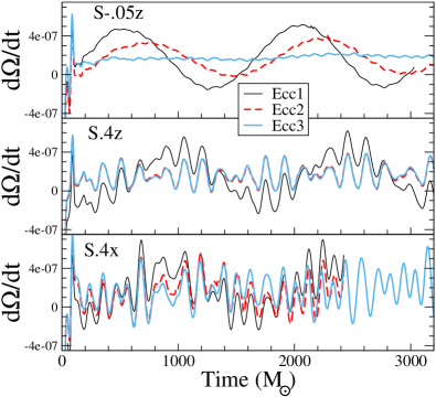
Figure 11: The derivative of the binary orbital frequency as a function of time for different levels of eccentriccity reduction for our three runs of interest. Note that $d\Omega/dt$ has units of $M_{\odot}^{-2}$.

For binary neutron stars, we initialize the first iteration of eccentricity removal, with $\dot{a}_{0}=0$ and use $\Omega_{0}$ determined from irrotational BNS initial data, based on the equilibrium condition in Eq. 38. Evolutions with these choices are labeled with the suffix “Ecc1”, and show noticable variations in the separation between the two NS, cf. the solid black lines in Fig. 10.

We compute the trajectories of the centers of mass of each star, as determined by Eq. 65, $\vec{c}_{1}(t)$ and $\vec{c}_{2}(t)$, and using the relative separation $\vec{r}=\vec{c}_{2}(t)-\vec{c}_{1}(t)$, compute the orbital frequency

$$\Omega(t)=\frac{|\vec{r}(t)\times\dot{\vec{r}}(t)|}{r(t)^{2}},$$ (68)

where an over-dot indicates a numerical time-derivative. Finally, we compute $\dot{\Omega}(t)$ and fit it to a function of the form

$$\dot{\Omega}(t)= A_{1}(t_{c}-t)^{-11/8}+A_{2}(t_{c}-t)^{-13/8}$$

$$+B_{0}\cos{(B_{1}t+B_{2}t^{2}+B_{3})}.$$ (69)

The power law parts of this fit represent the orbital decay due to the emission of gravitational waves, while the oscillatory part represents the eccentric part of the orbit. We then update $\Omega_{0}$ and $\dot{a}_{0}$ with the formulae (see Buonanno et al. (2011) for a detailed overview)

$$\Omega_{0}\leftarrow\Omega_{0}-\frac{B_{0}B_{1}}{4\Omega_{0}^{2}}\sin B_{3},$$ (70)

$$\dot{a}_{0}\leftarrow\dot{a}_{0}+\frac{B_{0}}{2\Omega_{0}}\cos B_{3}.$$ (71)

We repeat this procedure twice, resulting in simulations with suffix Ecc2 and Ecc3. Table 3 summarizes the orbital parameters for the individual simulations, and Figs. 10 and 11 illustrate the efficacy of the procedure through plots of separation and time-derivative of orbital frequency. The eccentricity is successfully reducued from $e\sim 1\%$ to $\sim 0.1\%$. After two eccentricity reduction iterations, variations in $\dot{\Omega}(t)$ are so small that they are no longer discernible from higher-frequency oscillations in $\dot{\Omega}(t)$, cf. Fig. 11.

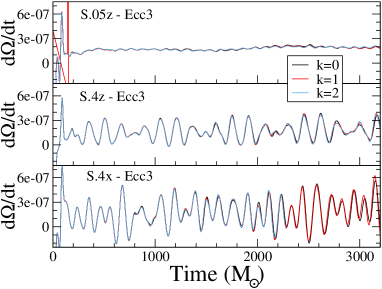
Figure 12: Convergence of $\dot{\Omega}(t)$. Shown are $\dot{\Omega}(t)$ at three different numerical resolutions ($k=0,1,2$) for the final, lowest-eccentricity initial data. The oscillations in $\dot{\Omega}(t)$ are evidently not caused by numerical truncation error. Note that $\dot{Omega}$ has units of $M_{\odot}^{-2}$.

The high freuqency oscillations in $\dot{\Omega}(t)$ are caused by the quasi-normal ringing of the neutron stars, as discussed in detail below in Sec. IV.5. Here, we only note that these oscillations are convergently resolved, cf. Fig. 12, and are therefore a genuine feature of our initial data. Figure 12 also confirms that the lowest resolution ($k=0$) gives adequate resolution for eccentricity removal.

The eccentricity removal algorithm attempts to isolate variations on the orbital time-scale as the signature of eccentricity. For S.4z - Ecc2, it reports $e=0.0005$ and for S.4z - Ecc3, $e=0.0002$. However, given the large amplitude of the QN mode ringing, we consider these estimates unreliable, and therefore quote an upper bound of 0.001 in Table 3. Similarly, for S.4x - Ecc3, the fitting reports $e=0.001$, and we quote a conservative upper bound of 0.002.

IV.3 Aligned spin BNS evolutions: NS Spin

In this section, we will discuss the measurement of spins during our evolutions for the non-precessing cases, S.4z and S-.05z. Aligned spin binaries do not precess. Combined with the low viscosity we expect the NS spins to stay approximately constant during the evolutions. These systems therefore serve as a test on our spin diagnostics during the evolutions. In this section, and through the rest of this paper, we always use the final eccentricity reduction, “Ecc3”. For brevity, we will omit the suffix “-Ecc3”, and refer to the runs simply as S-.05z, etc.

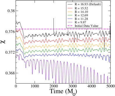
Figure 13: The spin measured on multiple coordinate spheres for the S.4z run.

We do not track the surface of the star during the evolution. Instead we simply evaluate the quasi-local spin of the stars on coordinate spheres in the frame comoving with the binary. We must therefore verify that the spin measured is largely independent of the radius of the sphere, and that it is maintained during the evolutions at the value consistent with that in the initial data. Figure 9 established that coordinate spheres can be used to extract the quasi-local spin in the initial data. Figure 13 shows the results for the high-spin simulation S.4x during the inspiral.

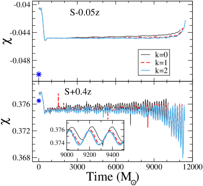
Figure 14: Neutron star spin during the two aligned-spin evolutions. Shown are three different numerical resolutions, $k=0$ (lowest), $k=1$, and $k=2$ (highest). The asterisk indicates the spin measured on the stellar surface in the initial data.

For coordinate spheres with radii $R=11.28M_{\odot}$ to $R=16.93M_{\odot}$ in grid coordinates, the spins remain roughly constant in time. The different extraction spheres yield spins that agree to about 1%, with a consistent trend that larger extraction spheres result in slightly larger spins (as already observed in the initial data). The horizontal dashed line in Fig. 13 indicates the spin measured on the stellar surface (i.e. not on a coordinate sphere) in the initial data. We thus find very good agreement between all spin measurements, and conclude that the quasi-local spin is reliable to about 1%.

The extraction sphere $R=9.87M_{\odot}$ in Fig. 13 intersects the outer layers of the neutron star. Because the quasi-local spin captures only the angular momentum within the extraction sphere, the value measured on $R=9.87M_{\odot}$ falls as our comoving grid-coordinates cause this coordinate sphere to slowly move deeper into the interior of the star. This behavior, again, is consistent with Fig. 9.

These tests of using multiple coordinate spheres were only run for about half of the inspiral – enough to establish that the method is robust. Subsequently, we report spins measured on the largest coordinate sphere, $R=16.93M_{\odot}$.

The full behavior of the spin during the inspiral is shown in figure 14 for both the S.4z and S-.05z runs. Comparing the spin at different resolutions, we note that the data for $k\!=\!1$ and $k\!=\!2$ are much closer to each other than compared to $k\!=\!0$, indicating numerical convergence. We note that the impact of numerical resolution (as shown in Fig. 14) is small compared to the uncertainty inherent from the choice of extraction sphere, cf. Fig. 13. We also note that for the first $10000M_{\odot}$ of the run, the measured spin behaves as a constant, as expected, albeit with some small oscillations. However, afterward, we notice the absolute value of the spin starts to decrease in both cases. Finally, we note that in both cases, the spin measured in the inital data on the stellar surface is within $\Delta\chi=0.008$ of the spin measured during the evolution.

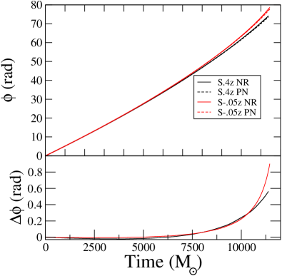
Figure 15: Accumulated orbital phase as a function of time for our anti-aligned, S-.05z, and aligned, S.4z, runs. The dashed lines are Taylor T4 PN simulations. The PN simulations were matched to NR in the intervals [1109,3956] and [2090,4904] respectively. Qualitatively, there is excellent agreement with the numerical data. The lower panel shows the difference $\Delta\phi(t)=\phi_{\rm NR}(t)-\phi_{\rm PN}(t)$.

Finally, we compute the orbital phase

$$\phi(t)=\int_{0}^{t}\Omega(t^{\prime})\,dt^{\prime},$$ (72)

where the orbital frequency $\Omega(t)$ is given by Eq. (68). The result is plotted in Fig. 15, along with the

Post-Newtonian prediction for the same binary parameters (spins, masses and initial orbital frequencies). We use the Taylor T4 model (see e.g.,Boyle et al. (2007)) at 3.5PN order expansion, with no tidal terms added, using the matching techniques described in Ossokine et al. (2015). We find excellent qualitative agreement in both cases, thereby giving additional evidence that our numerical simulations are working as expected. We do find large late time growth in the phase difference, however this is expected because we do not model tidal effects, which become increasingly important at late times, in our Post-Newtonian equations.

Figure 16 shows the gravitational waveforms for our two non-precessing simulations. We extract the waves on a sphere of radius $R=627M_{\odot}$.

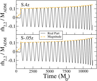
Figure 16: The gravitational waveforms for our anti-aligned, S-.05z, and aligned, S.4z runs. The black curve represents the real part of the waveform, $\Re(h_{2,2})$ while the orange curve represents the magnitude of the waveform.

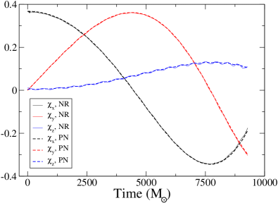
Figure 17: Spin-components of one of the neutron stars during the precessing simulation (thick, solid lines). The dotted and dashed lines represent the unmatched and matched PN results respectively. The agreement between PN and NR is good for both PN simulations. The orbital frequency was evolved using the Taylor T4 approximant. The matching was done in the interval [1892,4575].

IV.4 Precession

We now turn to the precessing simulation, S.4x. Figure 17 shows the components of the spin-vector $\vec{\chi}$ of one of the neutron stars, as a function of time. The quasi-local spin diagnostic returns a spin with nearly constant magnitude, varying only by $\pm 0.002$ around its average value $0.370$. The spin components clearly precess, with the dominant motion in the xy-plane (the initial orbital plane), with the simulation completing about 2/3 of a precession cycle. A z-component of the NS spin also appears, indicating precession of the neutron star spin out of the initial orbital plane.

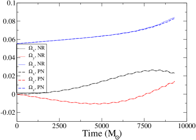
Figure 18: Components of the orbital frequency vector $\vec{\Omega}$. Thick solid lines represent the precessing BNS simulation and thin dashed lines represent the matched post-Newtonian simulations. The inclination reaches $\delta=0.34{\rm rad}$ at $t=7600M_{\odot}$.

Fig. 17 shows a comparison of spin precession between numerical relativity and Post-Newtonain theory. We perform this comparison using the matching tecnhique in Ossokine et al. (2015). This gives very good agreement between PN (dotted) and NR (solid) as shown by Fig. 17. The NS spins indeed precess as expected, thus confirming both the quality of quasi-local spin measures, as well as the performance of the PN equations. Note that z-component of the spin in the NR data undergoes oscillations that are unmodelled by PN. These occur on a timescale of half the orbital timescale. Similar effects were found in Ossokine et al. (2015). The origin of these oscillations remains unclear. The precession of the orbital angular frequency is shown in Fig. 18. We find substantial precession away from the initial direction of the orbital frequency $\vec{\Omega}_{0}\propto\hat{z}$, with the angle $\delta$ between $\vec{\Omega}(t)$ and the z-axis reaching $20^{\circ}$. Once again, the PN equations reproduce the precession features successfully.

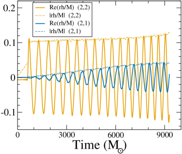
Figure 19: Gravitational waveforms of our precessing run. Shown are the $(l,m)=(2,2)$ and $(2,1)$ modes, as extracted in a spherical harmonic decomposition aligned with the z-axis. The emergence of the (2,1) mode indicates precession of the orbital plane away from the xy-plane.

Finally, Fig. 19 shows the (2,2) and the (2,1) spherical harmonic modes of the gravitational wave-strain extracted at an extraction surface of radius $R=647M_{\odot}$. The (l,m)=(2,1) mode would be identically zero for an equal-mass aligned spin binary with orbital frequency parallel to the z-axis, so the emergence of this mode once again indicates precession in this binary.

IV.5 Stellar Oscillations

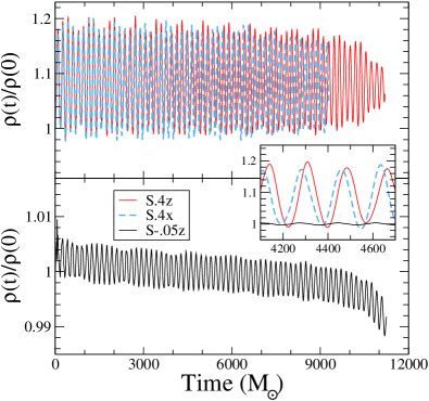
Figure 20: The maximum density $\rho(t)$ in each of our runs, normalized by the initial maximum density $\rho(0)$. The inset shows an enlargement of all three runs, illustrating that the oscillations are more pronounced in the high-spin simulations.

The rotating neutron stars constructed here show oscillations in the central density, as plotted in Fig. 20. In the low spin run, the density oscillations have a peak-to-peak amplitude of about 0.6%, whereas in the high-spin runs (S.4z and S.4x), the density oscillations reach a peak-to-peak amplitude of 20%. The two high-spin simulations show oscillations of nearly the same amplitude and frequency, therefore oscillating nearly in phase throughout the entire inspiral. The oscillation-period is about $177M_{\odot}\sim 0.87\rm{ms}$, i.e. giving a frequency of $1.15{\rm kHz}$. It remains constant throughout the inspiral. The low-spin run S-0.5z exhibits a slightly smaller oscillation period of about $P\approx 170M_{\odot}\approx 0.84\rm{ms}$, i.e. a frequency of $\approx 1.19{\rm kHz}$.

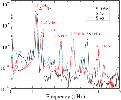
Figure 21: The Fourier transforms of the central density in all three of our runs. Labelled are the peak frequencies for the quasi-radial F mode and the $l=2$, ${}^{2}f$ mode.

To investigate the spectrum of the density oscillations, we perform a Fourier-transform on $\rho(t)$. The result is shown in Fig. 21. The Fourier-transform confirms the dominant frequencies just stated, and reveals several more frequency components ranging up to 4kHz. The high spin evolutions S.4z and S.4x exhibit identical freqencies for all five discernible peaks. In contrast, the low-spin evolution S-.05z shows different frequencies.

We interpret these features as a collection of excited quasi-normal modes in each neutron star. The modes are excited because the initial data is not precisely in equilibrium. For the two high-spin cases the neutron stars have similar spin, and therefore the same quasi-normal modes, whereas in the low-spin model, the quasi-normal mode frequencies differ due to the different magnitude of the spin.

To strengthen our interpretation, we consider the series of rotating, relativistic, $\Gamma=2$ polytropes computed by Dimmelmeier et al Dimmelmeier et al. (2006).

Ref. Dimmelmeier et al. (2006)’s model “AU3” has a central density of $1.074\times 10^{-3}M_{\odot}^{-2}$ and its rotation is quantified through the ratio of polar to equatorial radius, $r_{p}/r_{e}=0.780$. Meanwhile, our high-spin runs have a central density of $1.02\times 10^{-3}M_{\odot}^{-2}$ (measured as time-average of the data shown in Fig. 20) and from our initial data, we find $r_{p}/r_{e}\sim 0.8$. Given the similarity in these values, we expect Ref. Dimmelmeier et al. (2006)’s “AU3” to approximate our high-spin stars S.4x, S.4z. Ref. Dimmelmeier et al. (2006) reports a frequency of $f_{F}=1.283\rm{kHz}$ for the spherically symmetric ($\ell=0$) F-mode, and a frequency $f_{2f}=1.537\rm{kHz}$ for the axisymmetric $\ell=2$ mode ${}^{2}f$. These frequencies compare favorably with the two dominant frequencies in Fig. 21, $1.14\rm{kHz}$ and $1.42\rm{kHz}$.

Presumably, the small differences in these frequencies can be accounted for by the slight differences in stellar mass, radius, and rotation. Moreover, tidal interactions and orbital motion could factor in, as well. In our figure 21 we also see several other peaks at higher frequencies, which are reminiscent of the overtones and mode couplings in figure 10 of Dimmelmeier et al. (2006). If we identify our peak at $f_{H1}=4.03\rm{kHz}$ with the $H_{1}$ mode, then (in analogy to Dimmelmeier et al. (2006) Fig. 10), $f_{H1}-f_{F}=(4.03-1.14)\rm{kHz}=2.89\rm{kHz}$, and $2f_{F}=2.28\rm{kHz}$, two frequencies that are indeed present in our simulations. Although we find clear indications of axisymmetric $\ell=2$-modes, we note that their power is smaller by two orders of magnitude, compared to the spherically symmetric, dominant $F$ mode.

Turning to the low-spin run S.05z, we note that if, to first order, these frequencies scale like $f\sim\sqrt{\rho}$ (on dimensional grounds), then we expect to see $F=1.22\rm{kHz}$ and ${}^{2}f=1.49\rm{kHz}$. This is very close to what is seen.

The density oscillations discussed in this section are reflected in analogous oscillations in various other diagnostic quantities, for instance, the orbital frequency, Fig. 12 and the quasi-local spin as shown in Fig. 14. The dominant frequencies $1.14\rm{kHz}$ and $1.42\rm{kHz}$ can be robustly identified throughout our data analysis. In figure 22 we plot the Fourier transform of the density, the $(2,0)$ and $(2,2)$ gravitational wave strains, the orbital angular velocity time derivative $d\Omega/dt$ and the measured spin $\chi$ for the S.4z run. All show peaks in power at these two frequencies, $F\sim 1.14\rm{kHz}$ and ${}^{2}f\sim 1.4\rm{kHz}$. Gold et. al. Gold et al. (2012), in the simulation of close encounters in eccentric, irrotational, NSNS binaries, find an excited f-mode frequency of 1.586 kHz.

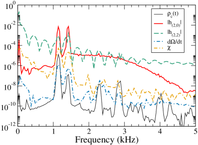
Figure 22: Fourier transforms of the central density $\rho_{c}(t)$, two modes of the magnitude of gravitational wave strain $(|h_{2,2}|$ and $|h_{2,0}|$), $\dot{\Omega}$ and $\chi$ for the S.4z run. All quantities show excess power at $1.14\rm{kHz}$ and $1.4\rm{kHz}$, corresponding to the frequencies of excited neutron star quasi-normal modes.

We believe that the stellar modes are excited because the initial data are not in perfect equilibrium. We expect the quasi-equilibrium approximations that enter the initial data formalism to become less valid at higher spins, consistent with our observation that the high spin models exhibit stronger oscillations. This interpretation is strengthened by additional simulations of neutron stars at larger separation. Increasing the intial separation by a factor 1.5, while keeping the same rotation parameter $\omega$ as in the S.4z-case, we find quasi-normal oscillations of similar amplitude than in S.4z. If the oscillations were caused by the neglect of tidal deformation, we would expect the amplitude to drop with the 3rd power of separation, inconsistent with our results.

Finally, we point out that the radial rotation profile, cf. Eq. (48) influences the amplitude of the induced quasi-normal oscillations. If the initial data is constructed with the rotation profile Eq. (49), instead of equation 48, then the amplitude of the density oscillations for high spin doubles. This further supports our conjecture that the origin of this mode comes from non-equilibrium initial data.

V Discussion

In this paper we implement Tichy’s method Tichy (2012) to construct binary neutron star initial data with arbitrary rotation rates. We demonstrate that our implementation is exponentially convergent, as expected for the employed spectral methods.

We measure the spin of the resulting neutron stars using the quasi-local angular momentum formalism Brown and York (1993); Cook and Whiting (2007); Lovelace et al. (2008); Owen (2007). The resulting angular momentum is found to be nearly independent on the precise choice of extraction sphere, cf. Fig. 9, and provides a means to define the quasi-local angular momentum of each neutron star to about 1%, both in the initial data and during the evolution, cf. Fig. 13. We are able to construct binary neutron star initial data with dimensionless angular momentum of each star as large as $\chi=S/M^{2}\sim 0.43$, both for the case of aligned spins, and also for a precessing binary where the initial neutron star spins are tangential to the initial orbital plane.

For irrotational BNS initial data sets, we find a quasi-local angular momentum of $\chi\sim 2\times 10^{-4}$, cf. Fig. 8. This spin is small enough that present waveform modeling studies for BNS (e.g. Bernuzzi et al. (2015); Baiotti et al. (2011, 2010)) are not yet limited by residual spin.

When evolving the initial data sets, the dimensionless spin measured in the initial data drops by about 0.004, and then remains constant through the 10 inspiral orbits for which we evolved the neutron star binaries. During these evolutions, we also demonstrated iterative eccentricity removal: By analyzing the orbital frequency $\Omega(t)$ during the first few orbits, we can correct the initial data parameters $\Omega_{0}$ and $\dot{a}_{0}$, and thus decrease the orbital eccentricity from $e\approx 0.01$ to $e\lesssim 0.001$.

For the precessing simulation S.4x, we find precession of the neutron star spin directions. The numerically established precession of the spin axes and of the orbital angular momentum agrees well with post-Newtonian predictions.

The rotating neutron stars constructed here exhibit clear signals of exciting quasi-normal modes. We are able to identify multiple modes in the Fourier spectrum of the central density. The amplitude of the excited quasi-normal modes increases steeply with rotation rate of the neutron stars. For S-.05z (spin magnitude $\chi=0.045$) the density oscillations have peak-to-peak amplitude of 0.6%, raising to 20% for the two runs with high spins (S.4x and S.4z).