SU(N) Multi-Skyrmions at Finite Volume

Abstract

We study multi-soliton solutions of the four-dimensional SU(N) Skyrme model by combining the hedgehog ansatz for SU(N) based on the harmonic maps of $S^{2}$ into $CP^{N-1}$ and a geometrical trick which allows to analyze explicitly finite-volume effects without breaking the relevant symmetries of the ansatz. The geometric set-up allows to introduce a parameter which is related to the ’t Hooft coupling of a suitable large $N$ limit, in which $N\rightarrow\infty$ and the curvature of the background metric approaches zero, in such a way that their product is constant. The relevance of such a parameter to the physics of the system is pointed out. In particular, we discuss how the discrete symmetries of the configurations depend on it.

1 Introduction

One of the most intriguing theoretical results in Quantum Field Theory (QFT henceforth) has been the realization that fermions can emerge out of purely bosonic Lagrangians as solitonic excitations (for a detailed review see [1]). The clearest demonstration that the importance of this result goes far beyond pure theoretical physics is given by the Skyrme theory [2] which is one of the most important models of nuclear and particle physics. The Skyrme term [2] allows the existence of static soliton solutions with finite energy, called Skyrmions (see  [3, 4, 5]) describing fermionic degrees of freedom (see [6, 7, 8, 9, 10, 11, 12] and references therein). The wide range of applications of the theory in other areas (such as astrophysics, Bose-Einstein condensates, nematic liquids, multi-ferric materials, chiral magnets and condensed matter physics in general [13, 14, 15, 16, 17, 18, 19, 20, 21, 22]) is well recognized by now. It is also worth to emphasize that the Skyrme model appears in a very natural way in the context of the AdS/CFT correspondence [23].

From the point of view of nuclear physics, it is very important to have analytic tools allowing to analyse the Skyrme model when interacting Skyrmions are present within bounded regions. This case is relevant whenever one wants to take into account the effects of the finite size on the topological properties of the Skyrmions themselves. It is commonly believed that many-nucleons systems (such as the ones occurring in nuclear pasta [24, 25]; for a review see [26]) are completely out of reach of the analytical techniques provided by soliton theory already in the $SU(2)$ case (while, at a first glance, the $SU(N)$ case is even worse). In particular, the task to compute physical parameters of such multi-nucleon systems with analytic multi-Skyrmionic configurations is believed to be completely hopeless.

Recently, the generalized hedgehog ansatz in the $SU(2)$ case, introduced in [27, 28, 29], allowed the construction of the first multi-Skyrmions at finite volume: namely, the first exact solutions of the Skyrme model representing interacting elementary Skyrmions with a non-trivial winding number, in which finite-volume effects can be explicitly taken into account (arriving at a good prediction for the compression modulus), was obtained [30]. The way to do this is to write the system in a modified “cylinder-like” metric whose curvature is parametrized by a length $R_{0}$. Then multi-Skyrmionic configurations look like necklaces of elementary Skyrmions interacting in bounded tube-shaped regions. The ground state of such multi-Skyrmions has the remarkable property that, although the BPS bound in terms of the winding cannot be saturated, a new topological charge exists which leads to a different BPS bound, which can instead be saturated.

In this paper, we consider the $SU(N)$ case. A very powerful technique to construct multi-Skyrmionic configurations in unbounded regions is given by an ansatz for $SU(N)$ Skyrmions introduced in [33] and [34], based on harmonic maps of $S^{2}$ into $CP^{N-1}$, which allowed the construction of many interesting numerical multi-Skyrmionic configurations. Here we will exploit the fact that the metric we use is spherically symmetric, just like flat space, so the harmonic map ansatz can be used also in the present case without modifications. We shall see that in the new metric the equations simplify with respect to those studied in [33] and [34]; in particular they become autonomous, thus techniques from dynamical systems theory become available. Thanks to the choice of the background geometry, a novel type of large $N$ limit becomes possible in which $N$ is large and the curvature is small in such a way that their product is constant. In this way one can see that both the effects of the curvature become negligible and the field equations remain autonomous (so that, in such a limit, one can kill the curvature of the metric but keeping all the advantages of the technique of [30]). It is also worth to emphasize that it is precisely the large $N$ limit which discloses in the clearest possible way the role of the Skyrme model as low energy limit of QCD. A non constructive proof of the existence of such nontrivial solutions is also provided and a few numerical solutions are exhibited as well.

This paper is organized as follows: in the second section, the $SU(2)$ case treated in [30] will be briefly reviewed in order to set the stage. In the third section, the ansatz for the Skyrmions will be described. In the fourth section, the general equations of motion are written down and the flat-large $N$ limit is discussed. In the fifth section, we study the system using techniques from the theory of dynamical systems; in particular, the stability of the fixed points in the $SU(3)$ case is analyzed, and their dependence on the geometric ’t Hooft parameter is discussed. In the sixth section, some nontrivial numerical solution of the equations of motion in the $SU(4)$ case will be studied. In the seventh section, some conclusions will be drawn. In the appendix, it is proved on general grounds that the equations of motion do have nontrivial solutions which can be interpreted as genuine $SU(N)$ Skyrmions.

2 Generalized hedgehog at finite volume: the $SU(2)$ case

In this section, the construction of analytic multi-Skyrmionic configurations in the $SU(2)$ case [30] will be shortly reviewed. The action of the four–dimensional Skyrme model is given by

$$S_{Sk}=\frac{K}{2}\int d^{4}x\sqrt{-g}\,\mathrm{Tr}\left(-\frac{1}{2}R^{\mu}R_{\mu}+\frac{\lambda}{16}F_{\mu\nu}F^{\mu\nu}\right),$$ (1)

$$K>0\ ,\ \ \ \lambda>0\ ,\,\ \ R_{\mu}:=U^{-1}\nabla_{\mu}U=R_{\mu}^{i}t_{i}\ ,\ \ F_{\mu\nu}:=\left[R_{\mu},R_{\nu}\right]\ ,$$

where the Planck constant and the speed of light have been set to $1$, and $K$ and $\lambda$ are the coupling constants. The $t^{i}$’s are the generators of the flavor group, which in this section is $SU(2)$. Notice that we allowed for curved metrics. The coupling constants $K$ and $\lambda$ are related to the couplings $F_{\pi}$ and $e$ used in [9] by

$$K=\frac{1}{4}F_{\pi}^{2},\quad K\lambda=\frac{1}{e^{2}}\ .$$

The non-linear sigma model term of the Skyrme action is necessary to take into account pions. The second term is the only covariant term leading to a well-defined Hamiltonian formalism in time which supports the existence of Skyrmions.

The field equations following from the above action are

$$\nabla^{\mu}R_{\mu}+\frac{\lambda}{4}\nabla^{\mu}[R^{\nu},F_{\mu\nu}]=0.$$ (2)

The following standard parametrization of the $SU(2)$-valued scalar $U(x^{\mu})$ will be adopted

$$U^{\pm 1}(x^{\mu})=Y^{0}(x^{\mu})\mathbf{1}_{2}\pm Y^{i}(x^{\mu})t_{i}\ ,\ \ \left(Y^{0}\right)^{2}+Y^{i}Y_{i}=1\ ,$$ (3)

where $\mathbf{1}_{2}$ is the $2\times 2$ identity matrix; to describe a spherically symmetric field configuration we use the hedgehog ansatz [28, 30]:

$$Y^{0}=\cos\alpha\ ,\ \ Y^{i}=\widehat{n}^{i}\sin\alpha\ ,\ \ \ \alpha=\alpha(x,t)\ ,$$ (4)

$$\widehat{n}^{1}=\sin\theta\cos\varphi\ ,\ \ \ \widehat{n}^{2}=\sin\theta\sin\varphi\ ,\ \ \ \widehat{n}^{3}=\cos\theta\ .$$ (5)

In order to mimic finite-volume effects without loosing the nice properties of the hedgehog ansatz we will consider the following curved background

$$ds^{2}=-dt^{2}+dx^{2}+R_{0}^{2}(d\theta^{2}+(\sin\theta)^{2}d\varphi^{2})\ ,\ \ -\frac{L}{2}\leq x\leq\frac{L}{2}\ ,$$ (6)

$$0\leq\theta\leq\pi\ ,\ 0\leq\varphi\leq 2\pi\ ,$$ (7)

where $L$ is the length of the $x-$interval. The total volume of space is $V=4\pi R_{0}^{2}L$. This geometry describes three-dimensional cylinders whose sections are $S^{2}$ spheres, so that parameter $R_{0}$ plays the role of the (finite) diameter of the transverse sections of the tube. The fact that this parameter replaces the radial variable $r$ in the metric also leads, as we will see, to considerable simplification of the equations of motion, even allowing to find exact solutions in the $SU(2)$ case. Moreover, the curvature of this metric is proportional to $1/R_{0}^{2}$. As it will be explained in the next sections, the explicit presence of this parameter in Eq. (6) together with the $N$ of $SU(N)$ allows to define a smooth flat limit in which $R_{0}\rightarrow\infty$ and so all the effects of the curvature disappear (however, the global topology of space remains cylindrical even in the flat limit and so it differs from the trivial $S^{3}$ topology of flat static unbounded Skyrmions). Thus, in a sense, the above metric is introduced just as a “regulator” whose local effects can be removed at the end. In the present context, “flat limit” really means

$$R_{0}\gg 1\ fm\ ,$$ (8)

so that, from the practical point of view, already when $R_{0}$ is around $100$ $fm$ all the effects of the curvature are negligible and, consequently, even in the flat limit in Eq. (8) finite volume effects will not disappear. It is also worth to emphasize that the well known result that elementary Skyrmions should be quantized as Fermions (which originally was derived on flat spaces) has been extended to space-times with compact orientable three-dimensional spatial sections in [38] (and the metric in Eq. (6) belongs to this class).

Since, at the end, we will be interested in the flat limit in Eq. (8), one may wonder whether it would be possible to start from the very beginning with a flat metric. In fact, as it has been shown in [30], the background metric in Eq. (6) is a very suitable tool to take into account finite volume effects (since the total spatial volume is finite) without breaking relevant symmetries of the hedgehog ansatz, with the additional advantage of simplifying the field equations. A further relevant advantage of the above background metric is that, unlike what happens in the usual unbounded case, it allows to define in a very transparent way a smooth large $N$ limit of the $SU(N)$ Skyrmions. Therefore, it is much more convenient to analyze the Skyrme theory first within the background metric in Eq. (6), and take the flat limit only later.

The effectiveness of such a choice for the metric is also shown by the results in [39] and [40] in which it has been shown that, unlike what happens in flat space, the equations for the Yang-Mills-Higgs system (in the sector with non-vanishing non-Abelian electric and magnetic charges) possess analytic solutions even in the case in which the Higgs coupling is non-zero.

With the above ansatz the Skyrme field equations reduce in the static case to the following scalar differential equation for the Skyrmion profile $\alpha$ [28]:

$$\left(1+\frac{2\lambda}{R_{0}^{2}}\,\sin^{2}\alpha\right)\overset{\cdot\cdot}{\alpha}-\frac{\text{sin}(2\alpha)}{R_{0}^{2}}\left(1-\lambda\left[\overset{\cdot}{\alpha}^{2}-\frac{\text{sin}^{2}\alpha}{R_{0}^{2}}\right]\right)=0$$ (9)

The winding number $W$ for such a configuration reads:

$$W=-\frac{1}{24\pi^{2}}\int\epsilon^{ijk}Tr\left(U^{-1}\partial_{i}U\right)\left(U^{-1}\partial_{j}U\right)\left(U^{-1}\partial_{k}U\right)=-\frac{2}{\pi}\int\left(\overset{\cdot}{\alpha}\sin^{2}\alpha\right)dx\ .$$ (10)

In the present case, the natural boundary conditions correspond to the choice:

$$\alpha\left(\frac{L}{2}\right)-\alpha\left(-\frac{L}{2}\right)=n\pi\ ,\ \ n\in\mathbb{Z}\ .$$ (11)

and with these boundary conditions the winding number takes the integer value $n$. These boundary conditions are unique in that they ensure $U(-\frac{L}{2})=(-1)^{n}U(\frac{L}{2})$, which correspond to bosonic and fermionic states for even and odd $n$, respectively.

Smooth solutions exist for any $n$ satisfying the above boundary conditions for a finite range $(-L/2,L/2)$. In particular multi-soliton solutions exist, which represent Skyrmions with winding number $n$ living in a finite spatial volume $V=4\pi R_{0}^{2}L$. It is worth to remark that the large $n$ limit in the present context is quite natural in order to consider thermodynamical properties of the multi-Skyrmions system and $n$ is the baryon number: obviously, a thermodynamical analysis only makes sense in the cases in which the number of particles is very large.

3 The hedgehog ansatz for SU(N)

Now we switch to the $SU(N)$ case with generic $N$. Our analysis will be based on the techniques introduced in [33, 34], which we shall now briefly describe. The hedgehog ansatz for $SU(N)$ spherically symmetric Skyrmions living in flat Minkowski metric

$$ds^{2}=-dt^{2}+dx^{2}+x^{2}(d\theta^{2}+(\sin\theta)^{2}d\varphi^{2})\ ,$$ (12)

is based on a suitable family of projectors from $S^{2}$ into $CP^{N-1}$ (see [41]). Such projectors $P(V)$ can be written as

$$P(V)=\frac{|V\rangle\langle V|}{|V|^{2}},$$ (13)

where $|V\rangle$ is an $N$-component complex vector of two complex variables $\xi$ and $\bar{\xi}$ which locally parametrize $S^{2}$, where $\xi=\tan(\theta/2)\,e^{i\varphi}$, and $|V|^{2}=\langle V|V\rangle$ . The first $P$ is constructed with a holomorphic $|V\rangle=|f(\xi)\rangle$ while the Gram-Schmidt procedure gives rise to the others. Indeed, $P_{+}$ can be found by its action on any vector $|v\rangle\in\mathbb{C}^{N}$ [41] as

$$P_{+}|v\rangle\ =\partial_{\xi}|v\rangle\ -|v\rangle\ \,\frac{\langle v|\,\partial_{\xi}|v\rangle}{|v|^{2}}.$$ (14)

Consequently, the other vectors $P_{+}^{k}|v\rangle\$ are determined inductively: $P_{+}^{k}|v\rangle\ =P_{+}(P_{+}^{k-1}|v\rangle\ )$.

Thus the operator $P_{k}$ corresponding to the family of vectors $|V\rangle\equiv|V_{k}\rangle=|P^{k}_{+}f\rangle$ (for $f=f(\xi)$) reads

$$P_{k}=P(P_{+}^{k}f)=\frac{|V_{k}\rangle\langle V_{k}|}{|V_{k}|^{2}},\hskip 14.22636pt\hskip 14.22636ptk=0,\dots,N-1,$$ (15)

where, due to the orthogonality of the projectors, we have $\sum_{k=0}^{N-1}P_{k}=1$.

Due to the holomorphy of $f$, the following identities of the above defined vectors can be proved [34]:

$$\langle V_{k}|V_{l}\rangle=0,\hskip 14.22636pt\hskip 14.22636pt\hskip 14.22636ptk\neq l,$$ (16)

$$\partial_{\bar{\xi}}|V_{k}\rangle=-|V_{k-1}\rangle\frac{|V_{k}|^{2}}{|V_{k-1}|^{2}},\hskip 14.22636pt\hskip 14.22636pt\partial_{\xi}\left(\frac{|V_{k-1}\rangle}{|V_{k-1}|^{2}}\right)=\frac{|V_{k}\rangle}{|V_{k-1}|^{2}}.$$ (17)

For $SU(N)$ the components of $|V_{N-1}\rangle=P_{+}^{N-1}|f\rangle$, up to an irrelevant overall factor which cancels in the projector, are functions of only $\bar{\xi}$.

The $SU(N)$ hedgehog ansatz defined in [33, 34] reads then

$$U =\exp\left\{i\alpha_{0}\left(P_{0}-\frac{\mathit{I}}{N}\right)+i\alpha_{1}\left(P_{1}-\frac{\mathit{I}}{N}\right)+\dots+i\alpha_{N-2}\left(P_{N-2}-\frac{\mathit{I}}{N}\right)\right\}$$

$$=e^{-i\alpha_{0}/N}(\mathit{I}+A_{0}P_{0})\,\,e^{-i\alpha_{1}/N}(\mathit{I}+A_{1}P_{1})\,\dots\,\,e^{-i\alpha_{N-2}/N}(\mathit{I}+A_{N-2}P_{N-2})\ ,$$ (18)

where we defined $A_{k}=e^{i\alpha_{k}}-1$. Such an ansatz involves the introduction of $N-1$ projectors and of $N-1$ profile functions $\alpha_{k}=\alpha_{k}(x)$, $k=0,\dots,N-2$; . Note that the projector $P_{N-1}$ is not included in the above formula since it is a linear combination of the others.

One of the main results in [33] and [34] has been to show that the above ansatz in Eq. (18), when inserted into the full Skyrme field equations in the case in which the background metric is the standard flat metric in spherical coordinates in Eq. (12), gives rise to a consistent set of $N-1$ coupled non-linear differential equations for the $N-1$ profiles $\alpha_{i}$. Moreover, such field equations can also be derived as stationary equations for the energy functional with respect to variations of the profiles. A close inspection of the computations in [34] shows that the main requirement in order for the ansatz to work is the $SO(3)$ invariance of the background metric. This then suggests that the above ansatz may also work in the finite-volume metric in Eq. (6) adopted in [30]. This is what we show in the next section.

4 Hedgehog ansatz for SU(N) at finite volume

In this section we switch back to the finite-volume $SO(3)$-invariant metric in Eq. (6). A direct computation shows that the ansatz in Eq. (18), when inserted into the full Skyrme field equations in this metric gives rise to a consistent system of $N-1$ coupled autonomous non-linear differential equations for the $N-1$ profiles $\alpha_{i}$ which is simpler than the flat non-autonomous system analyzed in [34] as it will be now discussed. Furthermore, also in the present case the field equations can be derived as stationary equations for the energy functional with respect to variations of the $\alpha_{j}$’s. It is worth emphasizing here that the explicit presence of the parameters $N$ and $R_{0}^{-2}L$ allows to consider a flat large $N$ limit in which the curvature is negligible and the product $NR_{0}^{-2}L$ remains constant. Hence, the present formalism is also relevant for people only interested in the Skyrme model on flat space-times. It is important to notice that in such a flat limit, while the effects of the curvature of the metric in Eq.(6) disappear, the effects of the cylindrical topology do not.

From now on we shall use the following energy $\left[E\right]$ and length $\left[L\right]$ units:

$$\left[E\right] =\frac{F_{\pi}}{4e}\approx 1\ GeV\ ,$$ (19)

$$\left[L\right] =\frac{2}{eF_{\pi}}\approx 0.6\ fm\ \Rightarrow$$ (20)

$$K=2\ ,\ \ \lambda=1\ .$$ (21)

Following the same steps of [34] in the new metric, one arrives at the following expressions for the winding number, the total energy of the $SU(N)$ hedgehog and the field equations respectively:

$$W=\frac{1}{2\pi}\sum_{i=0}^{N-2}\left(1+i\right)\left(N-i-1\right)\left.\left[F_{i}-\sin F_{i}\right]\right|_{x=-L/2}^{x=L/2}\ ,$$ (22)

$$E_{tot} =\frac{R_{0}^{2}}{6\pi}\int\,dx\,\left[-\frac{1}{N}\left(\sum_{i=0}^{N-2}\overset{\cdot}{\alpha}_{i}\right)^{2}+\sum_{i=0}^{N-2}\left(\overset{\cdot}{\alpha}_{i}\right)^{2}+\frac{1}{2R_{0}^{2}}\sum_{k=1}^{N-1}\left(\overset{\cdot}{\alpha}_{k}-\overset{\cdot}{\alpha}_{k-1}\right)^{2}D_{k}\right.$$

$$\left.+\frac{2}{R_{0}^{2}}\sum_{i=1}^{N-1}D_{i}+\frac{1}{4R_{0}^{4}}\left(D_{1}^{2}+D_{N-1}^{2}+\sum_{k=1}^{N-2}\left(D_{k}-D_{k+1}\right)^{2}\right)\right]\ ,$$ (23)

$$0 =-\frac{2(l+1)}{N}\sum_{i=0}^{N-2}\left(1+i\right)\overset{\cdot\cdot}{F}_{i}+\sum_{k=0}^{l}\sum_{i=k}^{N-2}\overset{\cdot\cdot}{F}_{i}+\frac{\left(l+1\right)\left(N-l-1\right)}{R_{0}^{2}}\left(1-\cos\left(F_{l}\right)\right)\overset{\cdot\cdot}{F}_{l}$$

$$+\frac{\left(l+1\right)\left(N-l-1\right)}{2R_{0}^{2}}\sin\left(F_{l}\right)\left(\overset{\cdot}{F}_{l}\right)^{2}-2\frac{\left(l+1\right)\left(N-l-1\right)}{R_{0}^{2}}\sin\left(F_{l}\right)$$

$$-\frac{\left(l+1\right)^{2}\left(N-l-1\right)^{2}}{R_{0}^{4}}\left(1-\cos\left(F_{l}\right)\right)\sin\left(F_{l}\right)$$

$$+\frac{\left(l+1\right)\left(N-l-1\right)\sin\left(F_{l}\right)}{2R_{0}^{4}}\left[l\left(N-l\right)\left(1-\cos\left(F_{l-1}\right)\right)+\left(l+2\right)\left(N-l-2\right)\left(1-\cos\left(F_{l+1}\right)\right)\right]\ \ \mathbf{,}$$ (24)

where we introduced the quantities

$$F_{k}=\alpha_{k}-\alpha_{k+1}\ ,\quad k=0,\ldots,N-3,\quad F_{N-2}=\alpha_{N-2},$$ (25)

$\overset{\cdot}{F}_{l}=dF_{l}/dx$, and we defined

$$D_{k}=k\left(N-k\right)\left(1-\cos\left(\alpha_{k}-\alpha_{k-1}\right)\right).$$ (26)

Notice that the winding number gets two different contributions (while in the Minkowski case it just gets one), as a consequence of the different topology of the cylinder-like metric we are using. Another important point is that when the parameter $R_{0}$ is very large the field equations (24) tend to linear equations, on the other hand when $R_{0}$ is small the nonlinear terms become very important. Thus, this parameter (more precisely, the quantity $1/R_{0}^{2}$) controls the nonlinearity of the theory, and thus it plays the rôle of an additional coupling constant. All the analyses we shall perform in the following will confirm the fact that the physics of the model crucially depends on it. More precisely, both the numerical analysis of Sect. 6 and the existence theorem of the appendix tell us that the global properties of the solutions of the system depend on the dimensionless parameter $R_{0}/L$, which controls the shape of the cylinder.

By comparing the present total energy in Eq. (23) and the field equations in Eq. (24) with the corresponding expressions in [34], the first of the advantages mentioned above in working within the metric in Eq. (6) is apparent. Namely, the field equations become an autonomous system which can, as such, be analyzed with the powerful tools of dynamical systems theory.

In the special case in which all the profiles are equal, i.e. $F_{l}=F,\,\,\forall\,\,l$ all the equations of the above system become proportional and equivalent to:

$$\overset{\cdot\cdot}{F}\left(1+\frac{(1-\text{cos}F)}{R_{0}^{2}}\right)-\frac{\text{sin}F}{2R_{0}^{2}}\left[4-\left(\overset{\cdot}{F}^{2}-\frac{2(1-\text{cos}F)}{R_{0}^{2}}\right)\right]=0$$ (27)

Upon setting $F=2\alpha$, this is precisely Eq. (9), valid in the $SU(2)$ case. This is to be expected since setting all the profiles to be equal corresponds to looking for solutions which are embeddings of the $SU(2)$ ones in $SU(N)$.

In the next sections we shall see numerically in some cases that the above system of equations does admit nontrivial solutions, i.e. solutions whose profiles are not equal nor proportional, while in the appendix we shall prove analytically the existence of such solutions. Such solutions have winding numbers which in general are nonvanishing, therefore can be interpreted as genuine $SU(N)$ multi-Skyrmion configurations.

4.1 The flat-large $N$ limit

As said, the formalism developed so far strongly relies on the usage of a spacetime whose spatial sections have a finite radius $R_{0}$, and whose curvature goes to zero as $R_{0}\rightarrow\infty$. In this section we will show that there is a natural way to accommodate this flat limit, which requires to take the large $N$ limit as well. The latter is a common tool in Quantum Field Theory, see e.g. [42] for a review.

The field equations in Eq. (24) can be rewritten as follows

$$0 =\frac{1}{N}\left(-2(l+1)\sum_{i=0}^{N-2}\left(1+i\right)\overset{\cdot\cdot}{F}_{i}+2N\sum_{k=0}^{l}\sum_{i=k}^{N-2}\overset{\cdot\cdot}{F}_{i}\right)+\frac{\left(N-l-1\right)}{\left(N-1\right)}\frac{\left(l+1\right)}{R^{2}}\left(1-\cos\left(F_{l}\right)\right)\overset{\cdot\cdot}{F}_{l}$$

$$+\frac{\left(N-l-1\right)}{\left(N-1\right)}\frac{\left(l+1\right)}{2R^{2}}\sin\left(F_{l}\right)\left(\overset{\cdot}{F}_{l}\right)^{2}-2\frac{\left(N-l-1\right)}{\left(N-1\right)}\frac{\left(l+1\right)}{R^{2}}\sin\left(F_{l}\right)$$

$$-\frac{\left(N-l-1\right)}{\left(N-1\right)^{2}}^{2}\frac{\left(l+1\right)^{2}}{R^{4}}\left(1-\cos\left(F_{l}\right)\right)\sin\left(F_{l}\right)$$

$$+\frac{\left(N-l-1\right)}{\left(N-1\right)}\frac{\left(l+1\right)\sin\left(F_{l}\right)}{2R^{4}}\left[l\frac{\left(N-l\right)}{\left(N-1\right)}\left(1-\cos\left(F_{l-1}\right)\right)+\left(l+2\right)\frac{\left(N-l-2\right)}{\left(N-1\right)}\left(1-\cos\left(F_{l+1}\right)\right)\right]\ \ \mathbf{,}$$ (28)

where we introduced the effective radius

$$R^{2}=\frac{R_{0}^{2}}{N-1}\ .$$ (29)

The nonlinear part of the field equations (28) behaves smoothly in the large $N$ limit provided also $R_{0}$ is large, so that $R$ is kept constant. More precisely:

$$N\rightarrow\infty\ ,\ R_{0}^{2}\rightarrow\infty\,|\ \ \underset{N\rightarrow\infty}{\lim}\frac{R_{0}^{2}}{N-1}=R^{2}=finite\,.$$ (30)

Hence, the proper way to consider the large $N$ limit is to simultaneously consider the flat limit $R_{0}^{2}\rightarrow\infty$ in such a way that the parameter $R^{2}$ in Eq. (29) remains finite. Since in the large $N$ limit in Eq. (30) the nonlinear part of the field equations Eq. (28) does not depend on $N$ and $R_{0}$ separately but only on the effective radius $R$ defined in Eq. (29), the quantity $1/R^{2}=(N-1)/R_{0}^{2}$ plays the rôle of a geometric (it defines a length scale) ’t Hooft coupling. Physically, the parameter $R^{2}$ in Eq. (29) represents the “effective area” available for each Skyrmion within each section of the tube.

In conclusion, one can see the metric defined in Eq. (6) just as a technical device in order to analyze multi-Skyrmionic configurations since, at the end, one can turn off all the effects of the curvature (keeping the cylindrical topology). In this limit, the solutions of the field equations represent multi-Skyrmionic configuration living in a flat tube-shaped region whose sections have a radius much bigger than the scale $R$.

When N is large the equations read:

$$0 =\frac{1}{N}\left(-2(l+1)\sum_{i=0}^{N-2}\left(1+i\right)\overset{\cdot\cdot}{F}_{i}+2N\sum_{k=0}^{l}\sum_{i=k}^{N-2}\overset{\cdot\cdot}{F}_{i}\right)+\frac{\left(l+1\right)}{R^{2}}\left(1-\cos\left(F_{l}\right)\right)\overset{\cdot\cdot}{F}_{l}$$

$$+\frac{\left(l+1\right)}{2R^{2}}\sin\left(F_{l}\right)\left(\overset{\cdot}{F}_{l}\right)^{2}-2\frac{\left(l+1\right)}{R^{2}}\sin\left(F_{l}\right)$$

$$-\frac{\left(l+1\right)^{2}}{R^{4}}\left(1-\cos\left(F_{l}\right)\right)\sin\left(F_{l}\right)$$

$$+\frac{\left(l+1\right)\sin\left(F_{l}\right)}{2R^{4}}\left[l\left(1-\cos\left(F_{l-1}\right)\right)+\left(l+2\right)\left(1-\cos\left(F_{l+1}\right)\right)\right]\ \ \mathbf{,}$$ (31)

The first two terms in the above equation (involving summations) describe the free part of the theory, while the rest (involving $R$) is responsible for interactions, therefore defines nontrivial dynamics. Therefore we find our prescription (30) a reasonable way to implement flat (large volume) limit within our formalism. In the next section we will demonstrate (for $N=3$), that the dynamics does depend on $R$.

5 Phase space portrait and geometrical ’t Hooft parameter

One of the strongest advantages of our formalism lies in the fact that we have an autonomous system of differential equations. The latter can be qualitatively described by its phase portrait, an important characteristic of which is the set of critical points. In particular if under some change of parameters the set of critical points remains the same (their number and their character), then one does not expect that dynamics of the system changes dramatically under the same change. On the contrary, if the number and/or character of the critical points changes, one may definitely say that the dynamics of the system is qualitatively different.

In this section we are going to study our system by using the tools of dynamical system theory (we will follow [43, 44]). In particular, we will analyze how changing the value of $R^{2}$ the number of the critical points of the dynamical system, as well as their linear stability properties, change.

For simplicity, we shall perform the analysis in the $SU(3)$ case. In this case we have two profiles, $F_{0}$ and $F_{1}$, and the equations of motion are given by:

$$\overset{{\cdot\cdot}}{F_{0}}\left(\frac{2}{3}+\frac{1}{2R^{2}}\left(1-\text{cos}F_{0}\right)\right)+\frac{1}{3}\overset{{\cdot\cdot}}{F_{1}}+\frac{\text{sin}F_{0}}{4R^{2}}\left[\overset{{\cdot}}{F_{0}}^{2}-4-\frac{2\left(1-\text{cos}F_{0}\right)}{R^{2}}+\frac{\left(1-\text{cos}F_{1}\right)}{R^{2}}\right] =0\ ,$$

$$\overset{{\cdot\cdot}}{F_{1}}\left(\frac{2}{3}+\frac{1}{2R^{2}}\left(1-\text{cos}F_{1}\right)\right)+\frac{1}{3}\overset{{\cdot\cdot}}{F_{0}}+\frac{\text{sin}F_{1}}{4R^{2}}\left[\overset{{\cdot}}{F_{1}}^{2}-4-\frac{2\left(1-\text{cos}F_{1}\right)}{R^{2}}+\frac{\left(1-\text{cos}F_{0}\right)}{R^{2}}\right] =0\ .$$ (32)

Notice that the two equations go one into the other by exchanging $F_{0}$ and $F_{1}$. We are going to exploit this symmetry.

In order to study critical points of the system (32), first of all we rewrite it as a system of first order equations as follows:

$$\frac{d}{dx}\vec{Z}=\vec{G}\left(\vec{Z}\right),$$ (33)

where

$$\vec{Z}\equiv\left[\begin{array}[]{c}\Delta\\ E\\ F_{0}\\ F_{1}\end{array}\right],\quad\vec{G}\left(\vec{Z}\right)=\left[\begin{array}[]{c}-\hat{a}^{-1}\left[\begin{array}[]{c}Q(F_{0},F_{1},\Delta)\\ Q(F_{1},F_{0},E)\end{array}\right]\\ \Delta\\ E\end{array}\right],$$ (34)

and we introduced the following notations for brevity

$$\hat{a}\equiv\left[\begin{array}[]{cc}\frac{2}{3}+\frac{1}{2}\frac{1-\cos{F_{0}}}{R^{2}}&\frac{1}{3}\\ \frac{1}{3}&\frac{2}{3}+\frac{1}{2}\frac{1-\cos{F_{1}}}{R^{2}}\end{array}\right],\quad Q(\xi,\eta,\theta)\equiv\frac{\text{sin}\xi}{4R^{2}}\left[\theta^{2}-4-\frac{2\left(1-\text{cos}\xi\right)}{R^{2}}+\frac{\left(1-\text{cos}\eta\right)}{R^{2}}\right].$$ (35)

Stationary points $\vec{Z_{*}}$ are defined by vanishing of the vector field $\vec{G}$, which defines the flow of the autonomous equation (33) in phase space:

$$\vec{G}\left(\vec{Z_{*}}\right)=0.$$ (36)

One can easily check that $\det{\hat{a}}>0$, therefore $\vec{Z_{*}}$ can be written as follows:

$$\vec{Z_{*}}=\left[\begin{array}[]{c}0\\ 0\\ F_{0}^{*}\\ F_{1}^{*}\end{array}\right]$$ (37)

where $F_{0}^{*}$ and $F_{1}^{*}$ are solutions of the following algebraic equations

$$\left\{\begin{array}[]{c}Q(F_{0}^{*},F_{1}^{*},0)=0\\ Q(F_{1}^{*},F_{0}^{*},0)=0\end{array}\right..$$ (38)

Equations (38) imply one of the three possibilities (the fourth possibility does not have real solutions):

1. $\text{sin}F_{0}=0$; $\text{sin}F_{1}=0$;

2. $\text{sin}F_{1}=0$; $-4-\frac{2\left(1-\text{cos}F_{0}\right)}{R^{2}}+\frac{\left(1-\text{cos}F_{1}\right)}{R^{2}}=0$;

3. $\text{sin}F_{0}=0$; $-4-\frac{2\left(1-\text{cos}F_{1}\right)}{R^{2}}+\frac{\left(1-\text{cos}F_{0}\right)}{R^{2}}=0$.

Linearizing (33) in the vicinity of the critical point $\vec{Z_{*}}$ we obtain

$$\frac{d\vec{\epsilon}}{dx}=J\vec{\epsilon},\quad\vec{\epsilon}\equiv\vec{Z}-\vec{Z_{*}},$$ (39)

where $J$ is the jacobian matrix of the diffeomorphism $\vec{Z}\mapsto\vec{G}(\vec{Z})$ taken at the point $\vec{Z_{*}}$

$$\hat{J}_{j,k}\equiv\frac{\partial{G}_{j}}{\partial Z_{k}}\bigg{|}_{\vec{Z}=\vec{Z_{*}}},\quad j,k=1,..4.$$ (40)

In order to analyze stability of the critical point $\vec{Z_{*}}$ i.e. in order to understand whether phase trajectories starting near this point “run away” exponentially or not, one has to check whether eigenvalues of $J$ have real part or they are purely imaginary.

Below we present a complete analysis of the critical points. Since in the algebraic equations (38) the unknowns $F_{0}$ and $F_{1}$ enter via sine and cosine, it is sufficient to consider critical points modulo $2\pi$.

5.1 Case 1

We identify the following four independent subcases:

$\bullet$ $F_{0}^{*}=0,F_{1}^{*}=0$;

$\bullet$ $F_{0}^{*}=\pi,F_{1}^{*}=\pi$;

$\bullet$ $F_{0}^{*}=0,F_{1}^{*}=\pi$;

$\bullet$ $F_{0}^{*}=\pi,F_{1}^{*}=0$.

5.1.1 Case $F_{0}^{*}=F_{1}^{*}=0$

In the (equal profile) case $F_{0}^{*}=F_{1}^{*}=0$ jacobian matrix is

$$J=\left[\begin{array}[]{cccc}0&0&\frac{2}{R^{2}}&-\frac{1}{R^{2}}\\ \vskip 6.0pt plus 2.0pt minus 2.0pt\cr 0&0&-\frac{1}{R^{2}}&\frac{2}{R^{2}}\\ \vskip 6.0pt plus 2.0pt minus 2.0pt\cr 1&0&0&0\\ \vskip 6.0pt plus 2.0pt minus 2.0pt\cr 0&1&0&0\end{array}\right]$$ (41)

whose four eigenvalues are:

$$\lambda_{1,2}=\pm\frac{1}{R},\qquad\lambda_{3,4}=\pm\frac{\sqrt{3}}{R}.$$ (42)

Therefore this fixed point is unstable; this property does not depend on $R$.

5.1.2 Case $F_{0}^{*}=F_{1}^{*}=\pi$

Also in this case we have equal profiles $F_{0}^{*}=F_{1}^{*}=\pi$. In this case the jacobian matrix is

$$J=\left[\begin{array}[]{cccc}0&0&-\frac{1}{2}\,{\frac{\left(2\,{R}^{2}+3\right)\left(2\,{R}^{2}+1\right)}{{R}^{2}\left({R}^{4}+4\,{R}^{2}+3\right)}}&\frac{1}{2}\,{\frac{2\,{R}^{2}+1}{{R}^{4}+4\,{R}^{2}+3}}\\ \vskip 6.0pt plus 2.0pt minus 2.0pt\cr 0&0&\frac{1}{2}\,{\frac{2\,{R}^{2}+1}{{R}^{4}+4\,{R}^{2}+3}}&-\frac{1}{2}\,{\frac{4\,{R}^{4}+8\,{R}^{2}+3}{{R}^{2}\left({R}^{4}+4\,{R}^{2}+3\right)}}\\ \vskip 6.0pt plus 2.0pt minus 2.0pt\cr 1&0&0&0\\ \vskip 6.0pt plus 2.0pt minus 2.0pt\cr 0&1&0&0\end{array}\right]$$ (43)

and the eigenvalues

$$\lambda_{1,2}=\pm\frac{i\sqrt{6}}{2}\,{\frac{\sqrt{\left({R}^{2}+3\right)\left(2\,{R}^{2}+1\right)}}{\left({R}^{2}+3\right)R}},\quad\lambda_{3,4}=\pm\frac{i\sqrt{2}}{2}\,{\frac{\sqrt{\left({R}^{2}+1\right)\left(2\,{R}^{2}+1\right)}}{\left({R}^{2}+1\right)R}}$$ (44)

are purely imaginary, therefore this point is stable for all $R$.

5.1.3 Case $F_{0}^{*}=0$, $F_{1}^{*}=\pi$

Now we consider $F_{0}^{*}=0$, $F_{1}^{*}=\pi$. In this case the jacobian matrix

$$J=\left[\begin{array}[]{cccc}0&0&\frac{1}{2}\,{\frac{\left(2\,{R}^{2}-1\right)\left(2\,{R}^{2}+3\right)}{{R}^{4}\left({R}^{2}+2\right)}}&{\frac{{R}^{2}+1}{{R}^{2}\left({R}^{2}+2\right)}}\\ \vskip 6.0pt plus 2.0pt minus 2.0pt\cr 0&0&-\frac{1}{2}\,{\frac{2\,{R}^{2}-1}{{R}^{2}\left({R}^{2}+2\right)}}&-\,{\frac{2{R}^{2}+1}{{R}^{2}\left({R}^{2}+2\right)}}\\ \vskip 6.0pt plus 2.0pt minus 2.0pt\cr 1&0&0&0\\ \vskip 6.0pt plus 2.0pt minus 2.0pt\cr 0&1&0&0\end{array}\right]$$ (45)

has the eigenvalues

$$\lambda_{1,2} =\pm\frac{\left(R^{2}+2\right)\sqrt{\sqrt{48R^{8}+120R^{6}+24R^{4}-48R^{2}+9}-3}}{2R^{2}},$$

$$\lambda_{3,4} =\pm\frac{i\left(R^{2}+2\right)\sqrt{\sqrt{48R^{8}+120R^{6}+24R^{4}-48R^{2}+9}+3}}{2R^{2}}$$ (46)

Unlike the previous cases, now the properties of this critical point change at a critical value of the parameter $R$. Indeed, while the eigenvalues $\lambda_{3}$ and $\lambda_{4}$ are always purely imaginary, $\lambda_{1}$ and $\lambda_{2}$ are purely imaginary only when $R<1/\sqrt{2}$. In this regime this critical point is stable. For $R\geq 1/\sqrt{2}$ instead the first two eigenvalues become real, therefore the fixed point becomes unstable. This is a nice example of how the stability properties change at a critical value of the parameter. Interestingly, the value of $R$ at which the transition happens is the same below which new fixed points appear (i.e. those occurring in cases 2 and 3 described above).

5.1.4 Case $F_{0}^{*}=\pi$, $F_{1}^{*}=0$

In this case the equations are exactly the same of case 3, only with $\delta$ and $\epsilon$ exchanged. The eigenvalues are therefore exactly the same so that the same discussion applies.

5.2 Cases 2 and 3

We now consider cases 2 and 3 in the above list. Since they are related by the exchange $F_{0}\leftrightarrow F_{1}$, they will have the same eigenvalues and hence the same stability properties. Let us then consider case 2:

$$\sin F_{1}=0;\qquad-4-\frac{2\left(1-\text{cos}F_{0}\right)}{R^{2}}+\frac{\left(1-\text{cos}F_{1}\right)}{R^{2}}=0.$$ (47)

One may immediately check that a real solution only exists for $R\leq 1/\sqrt{2}$, and it is given by

$$F_{1}^{*}=\pi,\qquad F_{0}^{*}=\arccos(2R^{2}),$$ (48)

modulo $2\pi$. For $R>1/\sqrt{2}$ this critical point disappears. The jacobian matrix reads

$$J=\left[\begin{array}[]{cccc}0&0&{\frac{\left(8\,{R}^{8}-14\,{R}^{4}+3\right)\left(2\,{R}^{2}+3\right)}{{R}^{2}\left(4\,{R}^{8}-12\,{R}^{4}+9\right)}}&-\frac{1}{2}\,{\frac{6\,{R}^{2}+3}{2\,{R}^{4}-3}}\\ {\vskip 6.0pt plus 2.0pt minus 2.0pt}0&0&-{\frac{8\,{R}^{8}-14\,{R}^{4}+3}{4\,{R}^{8}-12\,{R}^{4}+9}}&-\frac{1}{4}\,{\frac{12\,{R}^{4}-12\,{R}^{2}-9}{{R}^{2}\left(2\,{R}^{4}-3\right)}}\\ {\vskip 6.0pt plus 2.0pt minus 2.0pt}1&0&0&0\\ {\vskip 6.0pt plus 2.0pt minus 2.0pt}0&1&0&0\end{array}\right]$$ (49)

and its eigenvalues are:

$$\lambda_{1,2} = \pm\frac{\sqrt{2}}{4}{\frac{\sqrt{\left(2\,{R}^{4}-3\right)\left(2\,{R}^{2}+1\right)\left(16\,{R}^{4}+10\,{R}^{2}-3+\sqrt{256\,{R}^{8}+896\,{R}^{6}-284\,{R}^{4}-924\,{R}^{2}+441}\right)}}{\left(2\,{R}^{4}-3\right)R}}$$ (50)

$$\lambda_{3,4} = \pm\frac{\sqrt{2}}{4}{\frac{\sqrt{-\left(2\,{R}^{4}-3\right)\left(2\,{R}^{2}+1\right)\left(-16\,{R}^{4}-10\,{R}^{2}+\sqrt{256\,{R}^{8}+896\,{R}^{6}-284\,{R}^{4}-924\,{R}^{2}+441}+3\right)}}{\left(2\,{R}^{4}-3\right)R}}$$

In the whole range $R<1/\sqrt{2}$, the first two eigenvalues are purely imaginary, while $\lambda_{3}$ and $\lambda_{4}$ are real, therefore this critical point is unstable. At $R=1/\sqrt{2}$, $\lambda_{3}$ and $\lambda_{4}$ vanish.

5.3 Summary

The analysis we just performed discloses the crucial dependence of the dynamics of our system on the parameter $R$. In fact we saw that there is a critical value $R=1/\sqrt{2}$ at which the nature and the number itself of the critical points change. For $0<R\leq 1/\sqrt{2}$ and for $R>1/\sqrt{2}$ we have two qualitatively different phase portraits, thereby different dynamics. These are genuine finite volume effects (since the parameter $R$ represents the available surface per Baryon within the tube-shaped region) which can be disclosed only within the present framework.

In Fig.1 we present location of critical points for $R<1/\sqrt{2}$ and $R>1/\sqrt{2}$. As one can easily see, the two plots are qualitatively different: while the latter grid is invariant under the discrete group of reflections $Z_{2}\times Z_{2}$ about the axes $F_{0}$ and $F_{1}$, the former is not, that is the symmetry is broken. Moreover the former is sensitive to the particular value of $R$, while the latter is always the same for all $R>1/\sqrt{2}$. Finally, the concentration of different critical points changes as well, since some of them changed color (i.e. type) when $R$ passed through the critical value, while new (green) fixed points appeared.

These metamorphoses of the phase portrait hint at the presence of some sort of phase transition occurring at strong coupling (recall that $1/R^{2}$ plays the rôle of a coupling constant). It is interesting to notice that, in our units, this critical value is of the order of the $fm$, so although irrelevant from a flat limit perspective, it may have important consequences in view of applications to nuclear physics, where the dimensions of the tube-shaped region should be precisely of that order of magnitude in order to model an atomic nucleus [30].

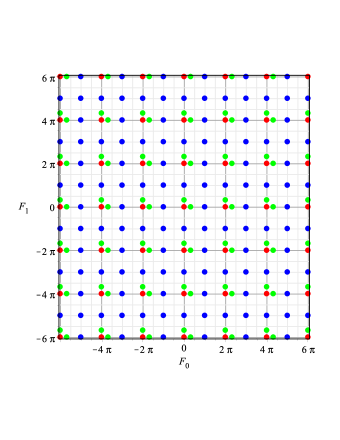
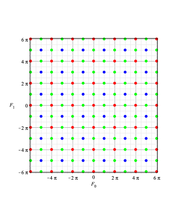
Figure 1: Location of critical points for $R<1/\sqrt{2}$ on the left and for $R>1/\sqrt{2}$ on the right. In the latter case the grid is independent on a particular choice of $R$, while for the former case we chose $R=\sqrt{\frac{\cos{1}}{2}}$. Blue points represent stable fixed points, red points represent “absolutely” unstable fixed points (i.e. all eigenvalues of the corresponding Jacobi matrix are real), while green points represent “softer” unstable fixed points (i.e two eigenvalues values are real and two imaginary).

6 Numerical Solutions: the $SU(4)$ case

In this section we perform a numerical study of the system in the $N=4$ case. In this case we have three profiles, $F_{0},F_{1},F_{2}$, and the equations of motion reduce to:

$$\overset{{\cdot\cdot}}{F_{0}}\left(1+\frac{2}{R_{0}^{2}}\left(1-\text{cos}F_{0}\right)\right)+\frac{2\overset{{\cdot\cdot}}{F_{1}}+\overset{{\cdot\cdot}}{F_{2}}}{3}+\frac{\text{sin}F_{0}}{R_{0}^{2}}\left[\overset{{\cdot}}{F_{0}}^{2}-4-\frac{6\left(1-\text{cos}F_{0}\right)}{R_{0}^{2}}+\frac{4\left(1-\text{cos}F_{1}\right)}{R_{0}^{2}}\right]=0,$$

$$\overset{{\cdot\cdot}}{F_{1}}\left(1+\frac{2}{R_{0}^{2}}\left(1-\text{cos}F_{1}\right)\right)+\frac{\overset{{\cdot\cdot}}{F_{0}}+\overset{{\cdot\cdot}}{F_{2}}}{2}+$$

$$+\frac{\text{sin}F_{1}}{R_{0}^{2}}\left[\overset{{\cdot}}{F_{1}}^{2}-4-\frac{8\left(1-\text{cos}F_{1}\right)}{R_{0}^{2}}+\frac{3\left(1-\text{cos}F_{0}\right)}{R_{0}^{2}}+\frac{3\left(1-\text{cos}F_{2}\right)}{R_{0}^{2}}\right]=0,$$

$$\overset{{\cdot\cdot}}{F_{2}}\left(1+\frac{2}{R_{0}^{2}}\left(1-\text{cos}F_{2}\right)\right)+\frac{\overset{{\cdot\cdot}}{F_{0}}+2\overset{{\cdot\cdot}}{F_{1}}}{3}+\frac{\text{sin}F_{2}}{R_{0}^{2}}\left[\overset{{\cdot}}{F_{2}}^{2}-4-\frac{6\left(1-\text{cos}F_{2}\right)}{R_{0}^{2}}+\frac{4\left(1-\text{cos}F_{1}\right)}{R_{0}^{2}}\right]=0.$$

The first and the second go one onto the other upon exchanging $F_{0}\leftrightarrow F_{2}$. We can exploit this symmetry to look for solutions which have $F_{0}=F_{2}\equiv F$ (another possibility allowed by the symmetry is to set $F_{0}=-F_{2}$ and at the same time $F_{1}=0$, however this would give vanishing winding number, so we do not consider it). Let us also call $F_{1}\equiv G$. In this case we get the two independent equations:

$$\overset{{\cdot\cdot}}{F}\left(1+\frac{2}{R_{0}^{2}}\left(1-\text{cos}F\right)\right)+\frac{\overset{{\cdot\cdot}}{F}+2\overset{{\cdot\cdot}}{G}}{3}+\frac{\text{sin}F}{R_{0}^{2}}\left[\overset{{\cdot}}{F}^{2}-4-\frac{6\left(1-\text{cos}F\right)}{R_{0}^{2}}+\frac{4\left(1-\text{cos}G\right)}{R_{0}^{2}}\right]=0,$$

$$\overset{{\cdot\cdot}}{G}\left(1+\frac{2}{R_{0}^{2}}\left(1-\text{cos}G\right)\right)+\overset{{\cdot\cdot}}{F}+\frac{\text{sin}G}{R_{0}^{2}}\left[\overset{{\cdot}}{G}^{2}-4-\frac{8\left(1-\text{cos}G\right)}{R_{0}^{2}}+\frac{6\left(1-\text{cos}F\right)}{R_{0}^{2}}\right]=0,$$

and the energy density (which is defined by $E=R_{0}^{2}(6\pi)^{-1}\int\mathcal{E}d\,x$) is given by:

$$\mathcal{E} =2\overset{{\cdot}}{F}^{2}+\overset{{\cdot}}{G}^{2}+2\overset{{\cdot}}{F}\overset{{\cdot}}{G}+\frac{1}{R_{0}^{2}}\left[3\left(\overset{{\cdot}}{F}^{2}+4\right)\left(1-\text{cos}F\right)+2\left(\overset{{\cdot}}{G}^{2}+4\right)\left(1-\text{cos}G\right)\right]+$$

$$+\frac{1}{R_{0}^{4}}\left[9\left(1-\text{cos}F\right)^{2}-12\left(1-\text{cos}F\right)\left(1-\text{cos}G\right)+8\left(1-\text{cos}G\right)^{2}\right].$$ (51)

Before solving the system we must choose a set of boundary conditions to impose on $F$ and $G$ in such a way to get solutions with a nontrivial winding number. Recall that we have to impose (anti-)periodic boundary conditions on the field $U$:

$$U\left(-\frac{L}{2}\right)=\pm\,U\left(\frac{L}{2}\right)$$ (52)

For simplicity we shall limit ourselves to the periodic case. According to the ansatz we are using the field can be written as:

$$U =\exp\left\{i\alpha_{0}\left(P_{0}-\frac{\mathit{I}}{4}\right)+i\alpha_{1}\left(P_{1}-\frac{\mathit{I}}{4}\right)+i\alpha_{2}\left(P_{2}-\frac{\mathit{I}}{4}\right)\right\}$$

$$=e^{-i\alpha_{0}/4}(\mathit{I}+A_{0}P_{0})\,\,e^{-i\alpha_{1}/4}(\mathit{I}+A_{1}P_{1})\,e^{-i\alpha_{2}/4}(\mathit{I}+A_{2}P_{2})\ .$$ (53)

It is convenient to use the second form. We notice that the matrix $U$ is diagonal in the basis $\{|V_{0}\rangle,|V_{1}\rangle,|V_{2}\rangle,\}$, therefore the above boundary condition is equivalent to its diagonal matrix elements. The diagonal matrix elements of $U$ are

$$\langle V_{0}|U|V_{0}\rangle=e^{\frac{i}{2}\,(2F+G)},\quad\langle V_{1}|U|V_{1}\rangle=e^{\frac{i}{2}\,G}=(\langle V_{2}|U|V_{2}\rangle)^{*}.$$ (54)

Thus the boundary conditions are satisfied if

$$F\left(-\frac{L}{2}\right)=F\left(\frac{L}{2}\right)+2m\pi,\quad m\in\mathbb{Z},\qquad G\left(-\frac{L}{2}\right)=G\left(\frac{L}{2}\right)+4n\pi,\quad n\in\mathbb{Z}.$$ (55)

With these conditions the winding number is given by

$$W=6\,m+8\,n.$$ (56)

We also need to impose conditions on the first derivative of $U$, i.e. of $F$ and $G$. We choose the simplest possibility which is compatible with the periodicity of the first derivative of $U$, i.e.

$$\overset{{\cdot}}{F}\left(-\frac{L}{2}\right)=\overset{{\cdot}}{F}\left(\frac{L}{2}\right),\qquad\overset{{\cdot}}{G}\left(-\frac{L}{2}\right)=\overset{{\cdot}}{G}\left(\frac{L}{2}\right).$$ (57)

We have solved numerically the system (6) with the boundary conditions (55) and (57), for some values of the integers $m$ and $n$, taking $R_{0}=L=1$, and we computed the energies of the solutions. The results are summarized in the tables below and in the one in sect. 6.1. We have allowed $m$ and $n$ to vary in a small range, beyond which our numerical procedure is not very accurate.

$m$	$n$	$W$	$E$	$m$	$n$	$W$	$E$	$m$	$n$	$W$	$E$
-1	1	2	26.68	1	0	6	11.43	1	1	14	43.87
-2	2	4	100.65	2	0	12	42.41	2	2	28	168.31
-3	3	6	228.42	3	0	18	92.08	3	3	42	376.07
				4	0	24	161.61

The energies are exactly the same if we change sign simultaneously to $m$ and $n$. There are sectors in which, to a very good approximation, the energy grows like the square of the modulus of the winding number, with different coefficients in different sectors. However, this is not true in all sectors, for example:

$m$	$n$	$W$	$E$
0	1	8	24.48
0	2	16	93.20

We notice that the solutions with the smallest winding numbers are not energetically favored, since to achieve small winding numbers both profiles must grow going along $x$ in opposite directions, while the smallest energy solutions are those where only one of the profile grows while the other oscillates and stays small, i.e. either $m$ or $n$ are different from zero, but not both. Notice also that increasing $n$ costs much more than increasing $m$, despite their contributions to the winding number being not so different.

In Figs.1-6 the plots of some solutions are reported.

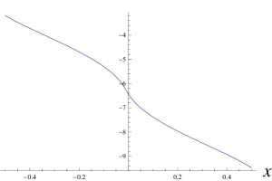
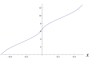
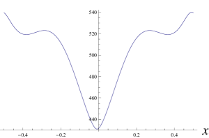
Figure 2: $F$,$G$ and $\mathcal{E}$ for $m=-1$, $n=1$.

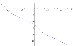
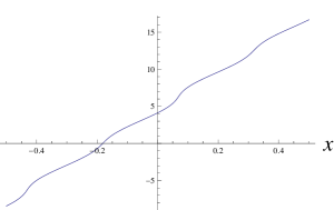
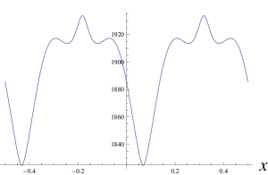
Figure 3: $F$,$G$ and $\mathcal{E}$ for $m=-2$, $n=2$.

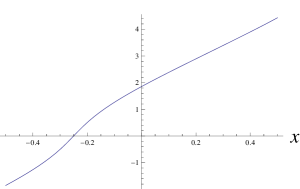
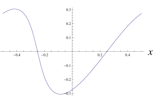
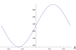
Figure 4: $F$,$G$ and $\mathcal{E}$ for $m=1$, $n=0$.

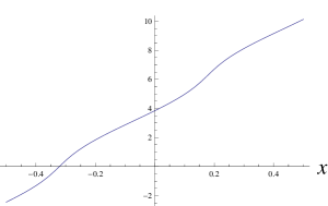
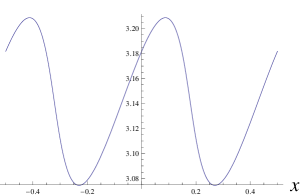
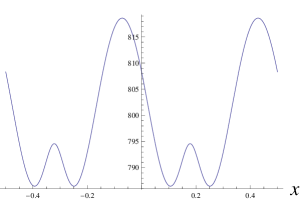
Figure 5: $F$,$G$ and $\mathcal{E}$ for $m=2$, $n=0$.

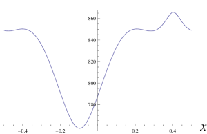
Figure 6: $F$,$G$ and $\mathcal{E}$ for $m=1$, $n=1$.

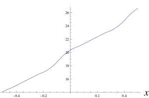
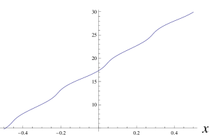
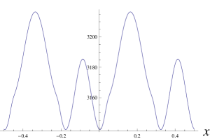
Figure 7: $F$,$G$ and $\mathcal{E}$ for $m=2$, $n=2$.

6.1 Comparison with the equal profile situation

If we impose that the profiles are equal, i.e $F=G\equiv F$, the equations of motion reduce of course to (27). In this case the same procedure followed above tells us that the boundary conditions to achieve a periodic $U$ are

$$F\left(-\frac{L}{2}\right)=F\left(\frac{L}{2}\right)+4m^{\prime}\pi,\quad m^{\prime}\in\mathbb{Z}$$ (58)

in which case the winding number is simply

$$W_{equal}=20\,m^{\prime}.$$ (59)

In order to compare the equal profile situation with the non equal profile one we have to consider cases with the same winding number. This is achieved if in the latter case we have $m=2n$. We did the computation in the two simplest cases, with $R_{0}=L=1$, and the results are:

$m^{\prime}$	$W_{equal}$	$E_{equal}$	$m$	$n$	$W$	$E$
1	20	82.67	2	1	20	82.67
2	40	325.70	4	2	40	325.57

We see that the energies are the same (in the second case the discrepancy is due to small numerical inaccuracies: the numerical computation for the $m=4$, $n=2$ case gave the winding number of the solutions to be 40.13, thus signalling such inaccuracies). Therefore, in topological sectors whose winding number is compatible with equal profile configurations, with the chosen values of the parameters, equal-profile solutions and non-equal profile ones are energetically equivalent.

6.2 Dependence on $R_{0}$

Besides the above analysis, which was performed at fixed $R_{0}$, we also studied what happens when this parameter is varied, considering for definiteness the lowest winding number case, i.e $m=-1,n=1$. We checked that when $R_{0}$ is increased the solutions tend to linear functions, in agreement with triviality of the dynamics for large radius. Instead, for values of $R_{0}$ (or $R_{0}/L$ if we allow also $L$ to vary) substantially smaller than $1$ the numerical procedure becomes unstable and the results unreliable. This is of course to be expected since lowering $R_{0}$ the non-linearity of the problem increases. This is in agreement with the bounds (89-94), which are more difficult to satisfy when $R_{0}$ is small, and trivial when $R_{0}$ is large.

In the small $R_{0}$ case a more sophisticated numerical analysis would therefore be needed. In particular it would be interesting to see whether at strong coupling non-equal profile solutions are energetically favored with respect to equal profile ones with the same winding number, as suggested by the fixed point analysis of section 5. Another interesting issue requiring a more accurate numerical work is the identification of a range of the parameters in which the dependence of the energy on the winding number is linear rather than quadratic. We hope to come back on these interesting issues in a future investigation.

7 Conclusions

In this paper the $SU(N)$ Skyrme model is studied in a tube-shaped geometry which allows to consider finite volume situations. The use of such a geometry allows to introduce a parameter which regulates the dynamics as a new (inverse) coupling constant. These simplifications, which make the system autonomous, allow us to perform a detailed study of the system using several techniques, i.e. dynamical systems, numerical solutions and rigorous existence theorems. All these analyses confirm the relevance of the parameter $R_{0}$ introduced by the metric on the dynamics of the system. As a further bonus, when combined with $N$ as $1/R^{2}=N/(R_{0})^{2}$, this parameter defines an effective ’t Hooft coupling. In the large $N$ limit in which such coupling is kept fixed, flat space-time is recovered. This effective ’t Hooft parameter determines the discrete symmetries of the Skyrmions configurations. These results clearly show that the present framework is a very promising tool to study interacting Skyrmions systems. A very interesting problem which we hope to analyse in a future publication is to extend the present analysis at finite temperature and/or chemical potential.

Acknowledgements

The authors would like to thank J. Zanelli for enlightening discussions and comments. This work has been funded by the Fondecyt grant 1120352. The Centro de Estudios Científicos (CECs) is funded by the Chilean Government through the Centers of Excellence Base Financing Program of Conicyt. M. K. acknowledges partial support from UniNA and Compagnia di San Paolo in the framework of the program STAR 2013.

Appendix: Existence of Solutions

In this appendix we prove analytically that non-trivial solutions which are not trivial embeddings of $SU(2)$ into $SU(N)$ (in which the profiles are not proportional) do indeed exist. We will focus for simplicity on the $SU(3)$ case but the same argument can be easily extended to the general case. The basic mathematical tool of this section is a well-known result of nonlinear functional analysis, the Schauder theorem (see for a detailed pedagogical review on mathematical tools to deal with non-linear partial differential equations [45]).

The statement of the Schauder theorem ([45, 46]) is the following. Let $S$ be a Banach space. Let $C$ a bounded closed convex set in $S$, and let $T$ be a compact operator from the Banach space $S$ into itself such that $T$ maps $C$ into itself:

$$T\left[.\right]:C\rightarrow C\ .$$ (60)

Then the map $T\left[.\right]$ has (at least) one fixed point in $C$. In other words, under the above hypotheses, there exists a solution to the equation

$$T\left[X\right]=X\ .$$ (61)

Let us recall the equations of motion for the $SU(3)$ case:

$$\overset{{\cdot\cdot}}{F_{0}}\left(\frac{2}{3}+\frac{1}{2R^{2}}\left(1-\text{cos}F_{0}\right)\right)+\frac{1}{3}\overset{{\cdot\cdot}}{F_{1}}+\frac{\text{sin}F_{0}}{4R^{2}}\left[\overset{{\cdot}}{F_{0}}^{2}-4-\frac{2\left(1-\text{cos}F_{0}\right)}{R^{2}}+\frac{\left(1-\text{cos}F_{1}\right)}{R^{2}}\right] =0\ ,$$ (62)

$$\overset{{\cdot\cdot}}{F_{1}}\left(\frac{2}{3}+\frac{1}{2R^{2}}\left(1-\text{cos}F_{1}\right)\right)+\frac{1}{3}\overset{{\cdot\cdot}}{F_{0}}+\frac{\text{sin}F_{1}}{4R^{2}}\left[\overset{{\cdot}}{F_{1}}^{2}-4-\frac{2\left(1-\text{cos}F_{1}\right)}{R^{2}}+\frac{\left(1-\text{cos}F_{0}\right)}{R^{2}}\right] =0\ .$$ (63)

We want to prove that the system in Eqs. (62) and (63) admits non-trivial solutions in which the profiles $F_{0}$ and $F_{1}$ are not proportional. In order to achieve this goal, let us rewrite it as coupled integral equations (for notational simplicity in this section we shall consider $x\in[0,L]$ instead of $x\in[-L/2,L/2]$, since everything just depends on the length $L$ of the tube):

$$F_{0}\left(x\right)=a_{0}+b_{0}x-\int_{0}^{x}H_{0}\left(s\right)ds\ ,$$ (64)

$$F_{1}\left(x\right)=a_{1}+b_{1}x-\int_{0}^{x}H_{1}\left(s\right)ds\ ,$$ (65)

where

$$H_{0}\left(s\right) =\,\int_{0}^{s}\,A_{0}\left\{\frac{\text{sin}F_{0}\left(\rho\right)}{4R^{2}}h_{0}\left(\rho\right)+\frac{1}{3}\overset{{\cdot\cdot}}{F_{1}}\left(\rho\right)\right\}d\rho\ ,$$ (66)

$$H_{1}\left(s\right) =\,\int_{0}^{s}\,A_{1}\left\{\frac{\text{sin}F_{1}\left(\rho\right)}{4R^{2}}h_{1}\left(\rho\right)+\frac{1}{3}\overset{{\cdot\cdot}}{F_{0}}\left(\rho\right)\right\}d\rho\ ,$$ (67)

$$h_{0}\left(\rho\right) =\left[\overset{{\cdot}}{F_{0}}^{2}-4-\frac{2\left(1-\text{cos}F_{0}\left(\rho\right)\right)}{R^{2}}+\frac{\left(1-\text{cos}F_{1}\left(\rho\right)\right)}{R^{2}}\right]\ ,\$$ (68)

$$h_{1}\left(\rho\right) =\left[\overset{{\cdot}}{F_{1}}^{2}-4-\frac{2\left(1-\text{cos}F_{1}\left(\rho\right)\right)}{R^{2}}+\frac{\left(1-\text{cos}F_{0}\left(\rho\right)\right)}{R^{2}}\right],$$ (69)

$$A_{i} =\left(\frac{2}{3}+\frac{1}{2\,R^{2}}\left(1-\cos\,F_{i}\right)\right)^{-1},\quad i=0,1$$ (70)

where $\overset{{\cdot}}{F_{i}}=\frac{dF}{d\rho}$, $i=0,1$, and $a_{i}$ and $b_{i}$ represent the initial data for the two profiles $F_{0}$ and $F_{1}$ and their derivatives at $x=0$. It is a trivial computation to show that the above system of integral equation is equivalent to the system in Eqs. (62) and (63). The system in Eqs. (64) and (65) can be written as a fixed point condition for the following vectorial operator $\overrightarrow{T}$ acting component-wise on pairs of $C^{2}$ functions $\overrightarrow{F}\left(x\right)=\left(F_{0}\left(x\right),F_{1}\left(x\right)\right)$:

$$\overrightarrow{T} :C^{2}\left[0,L\right]\times C^{2}\left[0,L\right]\rightarrow C^{2}\left[0,L\right]\times C^{2}\left[0,L\right]\ ,$$

$$\overrightarrow{F}\left(x\right) =\left(F_{0}\left(x\right),F_{1}\left(x\right)\right)\in C^{2}\left[0,L\right]\times C^{2}\left[0,L\right]\ ,$$

$$\overrightarrow{T}\left[F_{0},F_{1}\right]=\overrightarrow{T}\left[\ \overrightarrow{F}\left(x\right)\right]=\left(T_{0}\left(x\right),T_{1}\left(x\right)\right)\ ,$$ (71)

with

$$T_{0}\left(x\right) =a_{0}+b_{0}x-\int_{0}^{x}H_{0}\left(s\right)ds\ \ ,$$ (72)

$$T_{1}\left(x\right) =a_{1}+b_{1}x-\int_{0}^{x}H_{1}\left(s\right)ds\ \ ,$$ (73)

where the functions $H_{i}\left(s\right)$ are defined in Eqs. (66), (67), (68) and (69). It is then obvious that the system in Eqs. (64) and (65) can be written as the following fixed-point condition

$$\overrightarrow{F}\left(x\right)=\overrightarrow{T}\left[\ \overrightarrow{F}\left(x\right)\right]\ ,$$ (74)

where the operator $\overrightarrow{T}$ has been defined in Eqs. (71), (72) and (73). Hence, now the task is to define $\overrightarrow{T}$ as a compact operator from a bounded closed convex sub-set of a Banach space into itself.

In order to achieve this goal, first of all let us define the following metric into the space $C^{2}\left[0,L\right]\times C^{2}\left[0,L\right]$:

$$d\left(\overrightarrow{F},\overrightarrow{G}\right) =\underset{x\in\left[0,L\right]}{\sup}\left|F_{0}(x)-G_{0}(x)\right|+\underset{x\in\left[0,L\right]}{\sup}\left|\frac{dF_{0}}{dx}-\frac{dG_{0}}{dx}\right|+\underset{x\in\left[0,L\right]}{\sup}\left|\frac{d^{2}F_{0}}{dx^{2}}-\frac{d^{2}G_{0}}{dx^{2}}\right|+$$

$$+\underset{x\in\left[0,L\right]}{\sup}\left|F_{1}(x)-G_{1}(x)\right|+\underset{x\in\left[0,L\right]}{\sup}\left|\frac{dF_{1}}{dx}-\frac{dG_{1}}{dx}\right|+\underset{x\in\left[0,L\right]}{\sup}\left|\frac{d^{2}F_{1}}{dx^{2}}-\frac{d^{2}G_{1}}{dx^{2}}\right|\ ,$$ (75)

$$\overrightarrow{F}\left(x\right) =\left(F_{0}\left(x\right),F_{1}\left(x\right)\right)\ ,\ \overrightarrow{G}\left(x\right)=\left(G_{0}\left(x\right),G_{1}\left(x\right)\right)\ \in C^{2}\left[0,L\right]\times C^{2}\left[0,L\right]\ .$$

With respect to this metric, which is induced by a norm, the space $C^{2}\left[0,L\right]\times C^{2}\left[0,L\right]$ is a Banach space which we will call $S$.

The next task to apply the Schauder theorem is to define a bounded closed convex sub-set $C$ of the Banach space defined above (using the metric in Eq. (75)) such that $\overrightarrow{T}$ maps $C$ into itself. Let us define $C$ as

$$C \equiv\left\{\overrightarrow{F}\left(x\right)=\left(F_{0}\left(x\right),F_{1}\left(x\right)\right)\in\left.S\right|\ \forall x\in\left[0,L\right]\ \right.\ \left|F_{0}(x)-a_{0}\right|\leq B\ ,\ \left|F_{1}(x)-a_{1}\right|\leq B\ \ ,$$ (76)

$$\left.\ \left|\frac{dF_{0}}{dx}\right|\leq B\ ,\ \ \left|\frac{d^{2}F_{0}}{dx^{2}}\right|\leq B\ ,\ \ \left|\frac{dF_{1}}{dx}\right|\leq B\ ,\ \left|\frac{d^{2}F_{1}}{dx^{2}}\right|\leq B\right\}\ ,\quad\ \ \ B\in\mathbb{R}_{+}\ ,$$

where $a_{i}$ are the initial data appearing in Eqs. (64) and (65) so that $C$ is closed by definition. It is easy to see that $C$ is bounded as well, since from the definition of $C$ it follows that

$$\left|F_{0}(x)\right| \leq B+\left|a_{0}\right|\ ,\ \left|\frac{dF_{0}}{dx}\right|\leq B\ ,\ \left|\frac{d^{2}F_{0}}{dx^{2}}\right|\leq B\ ,$$ (77)

$$\left|F_{1}(x)\right| \leq B+\left|a_{1}\right|\ ,\ \left|\frac{dF_{1}}{dx}\right|\leq B\ ,\ \left|\frac{d^{2}F_{1}}{dx^{2}}\right|\leq B\ ,$$ (78)

which clearly implies that there exists $M$ such that $d(\overrightarrow{F},\overrightarrow{G})\leq M$, given any two functions $\overrightarrow{F},\overrightarrow{G}\in C$. It remains to prove that $C$ is convex, i.e. to check that if $\overrightarrow{F}\left(x\right)$ and $\overrightarrow{G}\left(x\right)$ both belong to $C$ then also $\theta\overrightarrow{F}\left(x\right)+\left(1-\theta\right)\overrightarrow{G}\left(x\right)$ belongs to $C$, $\forall\,\,\theta\in\left[0,1\right]$. This can be seen as follows:

$$\left|\theta F_{1}\left(x\right)+\left(1-\theta\right)G_{1}\left(x\right)-a_{1}\right| \leq\left|\theta\left(F_{1}\left(x\right)-a_{1}\right)\right|+\left|\left(1-\theta\right)\left(G_{1}\left(x\right)-a_{1}\right)\right|\leq\theta B+\left(1-\theta\right)B\leq B\ ,$$ (79)

$$\left|\theta F_{0}\left(x\right)+\left(1-\theta\right)G_{0}\left(x\right)-a_{0}\right| \leq\left|\theta\left(F_{0}\left(x\right)-a_{0}\right)\right|+\left|\left(1-\theta\right)\left(G_{0}\left(x\right)-a_{0}\right)\right|\leq\theta B+\left(1-\theta\right)B\leq B\ ,$$ (80)

while the conditions on the derivatives are trivially satisfied.

Thus, $C$ is closed, bounded and convex. The requirement that $\overrightarrow{T}$ maps $C$ into itself will impose some constraints on the parameters, as we shall see shortly.

From the definition of $C$ in Eq. (76) we deduce the inequalities

$$\underset{x\in\left[0,L\right]}{\sup}\left|H_{0}\left(x\right)\right| \leq L\left\{\frac{B}{2}+\frac{3}{8R^{2}}\left[B^{2}+4+\frac{6}{R^{2}}\right]\right\}\ ,$$ (81)

$$\underset{x\in\left[0,L\right]}{\sup}\left|H_{1}\left(x\right)\right| \leq L\left\{\frac{B}{2}+\frac{3}{8R^{2}}\left[B^{2}+4+\frac{6}{R^{2}}\right]\right\}\ ,$$ (82)

$$\underset{x\in\left[0,L\right]}{\sup}\left|\frac{dH_{0}}{dx}\right| \leq\frac{B}{2}+\frac{3}{8R^{2}}\left[B^{2}+4+\frac{6}{R^{2}}\right]\ ,$$ (83)

$$\underset{x\in\left[0,L\right]}{\sup}\left|\frac{dH_{1}}{dx}\right| \leq\frac{B}{2}+\frac{3}{8R^{2}}\left[B^{2}+4+\frac{6}{R^{2}}\right]\ ,$$ (84)

(where we used the fact that $A_{i}\leq 3/2$), which will be needed later.

The next task to apply the Schauder theorem is to prove that $\overrightarrow{T}$ is a compact operator. To do this we advocate the Ascoli-Arzelà theorem, which states that if a sequence of functions (defined on a compact metric space) $\left\{f_{n}\right\}$ is uniformly bounded and equicontinuous, then a convergent subsequence can be extracted from it. Thus compactness of $\overrightarrow{T}$ is equivalent to the statement that if $\overrightarrow{F}_{n}\left(x\right)=\left(F_{0}^{n}\left(x\right),F_{1}^{n}\left(x\right)\right)$ is a sequence in $C$, then the sequence $\overrightarrow{T}\left[\ \overrightarrow{F}_{n}\left(x\right)\right]=\left(T_{0}\left(n;x\right),T_{1}\left(n;x\right)\right)$ is uniformly bounded and equicontinuous.

Uniform boundedness can be proved as follows:

$$\left|T_{0}\left(n;x\right)\right|=\left|a_{0}+b_{0}x-\int_{0}^{x}H_{0}\left(n;s\right)ds\right|\leq\left|a_{0}\right|+\left|b_{0}L\right|+L\underset{x\in\left[0,L\right]}{\sup}\left|H_{0}\left(n;x\right)\right|\ .$$

and therefore, from Eq. (81), one gets:

$$\left|T_{0}\left(n;x\right)\right|\leq\left|a_{0}\right|+\left|b_{0}L\right|+L^{2}\left\{\frac{B}{2}+\frac{3}{8R^{2}}\left[B^{2}+4+\frac{6}{R^{2}}\right]\right\}\ ,$$ (85)

and, similarly, for $\left|T_{1}\left(n;x\right)\right|$:

$$\left|T_{1}\left(n;x\right)\right|\leq\left|a_{1}\right|+\left|b_{1}L\right|+L^{2}\left\{\frac{B}{2}+\frac{3}{8R^{2}}\left[B^{2}+4+\frac{6}{R^{2}}\right]\right\}\ .$$ (86)

Now, the sequence of images $\overrightarrow{T}\left[\ \overrightarrow{F}_{n}\left(x\right)\right]$ has to belong to $C$ as well. As it always happens (see [45] and [46]) this will give some constraints on the range of the initial data as well as on the parameters $B$, $L$ and $R$ since, from the definition of $C$, one has to require that for any $n$

$$\left|T_{0}\left(n;x\right)-a_{0}\right| \leq B\ ,~{}\left|\frac{dT_{0}\left(n;x\right)}{dx}\right|=\left|b_{0}-H_{0}\left(n;x\right)\right|\leq B\ ,\ \left|\frac{d^{2}T_{0}\left(n;x\right)}{dx^{2}}\right|=\left|\frac{dH_{0}\left(n;x\right)}{dx}\right|\leq B\ ,$$ (87)

$$\left|T_{1}\left(n;x\right)-a_{1}\right| \leq B,~{}\left|\frac{dT_{1}\left(n;x\right)}{dx}\right|=\left|b_{1}-H_{1}\left(n;x\right)\right|\leq B\ ,\ \left|\frac{d^{2}T_{1}\left(n;x\right)}{dx^{2}}\right|=\left|\frac{dH_{1}\left(n;x\right)}{dx}\right|\leq B\ .$$ (88)

Consequently, as it can be easily seen comparing Eqs. (87), (88), (76), (77) and (78) with Eqs. (81), (82), (83), (84), (85) and (86), the following constraints arise:

$$\left|b_{0}L\right|+L^{2}\left\{\frac{B}{2}+\frac{3}{8R^{2}}\left[B^{2}+4+\frac{6}{R^{2}}\right]\right\} \leq B\ ,$$ (89)

$$\left|b_{1}L\right|+L^{2}\left\{\frac{B}{2}+\frac{3}{8R^{2}}\left[B^{2}+4+\frac{6}{R^{2}}\right]\right\} \leq B\ ,$$ (90)

$$\left|b_{0}\right|+L\left\{\frac{B}{2}+\frac{3}{8R^{2}}\left[B^{2}+4+\frac{6}{R^{2}}\right]\right\} \leq B\ ,$$ (91)

$$\left|b_{1}\right|+L\left\{\frac{B}{2}+\frac{3}{8R^{2}}\left[B^{2}+4+\frac{6}{R^{2}}\right]\right\} \leq B\ ,$$ (92)

$$\frac{B}{2}+\frac{3}{8R^{2}}\left[B^{2}+4+\frac{6}{R^{2}}\right] \leq B\ \ ,$$ (93)

$$\frac{B}{2}+\frac{3}{8R^{2}}\left[B^{2}+4+\frac{6}{R^{2}}\right] \leq B\ .$$ (94)

Therefore, in order for this theorem to work, the length $L$ of the tube-shaped region in which these multi-Skyrmions are living cannot exceed the bounds defined in Eqs. (89) and (90) (indeed, if $L$ is too large, the bounds will be violated at a certain point.). It is also to be noticed that one cannot obtain a very large value for the allowed $L$ by increasing $B$ since the left hand sides of Eqs. (89) and (90) increase faster than the right hand sides. Moreover, the situation gets worse if $R^{2}$ is very small (as all the above inequalities are violated at a certain point). However, if $R$ is large (namely, in the flat limit), Eqs. (93) and (94) are always satisfied and Eqs. (91) and (92) become mild constraints on the initial data. On the other hand, it is trivial to see that it is always possible to choose the initial data and $B$, $L$ and $R$ in such a way that all the above inequalities are fulfilled.

The second step to prove that $T$ is compact is to show that if $\overrightarrow{F}_{n}\left(x\right)=\left(F_{0}^{n}\left(x\right),F_{1}^{n}\left(x\right)\right)$ is a sequence in $C$ then the sequence $\overrightarrow{T}\left[\ \overrightarrow{F}_{n}\left(x\right)\right]$ is equicontinuous. To show this, we must evaluate, for a generic $n$, the absolute values of following differences:

$$\left|T_{0}\left(n;x\right)-T_{0}\left(n;y\right)\right| =\left|b_{0}\left(x-y\right)+\int_{x}^{y}H_{0}\left(n;s\right)ds\right|\ ,$$ (95)

$$\left|T_{1}\left(n;x\right)-T_{1}\left(n;y\right)\right| =\left|b_{1}\left(x-y\right)+\int_{x}^{y}H_{1}\left(n;s\right)ds\right|\ ,$$ (96)

where $0<x<y<L$. After trivial manipulations (which use the fact that all the functions $\overrightarrow{F}_{n}\left(x\right)$ belong to $C$ and consequently Eqs.(77) and (78) are satisfied) one arrives at

$$\left|T_{0}\left(n;x\right)-T_{0}\left(n;y\right)\right| \leq\left|x-y\right|\left[\left|b_{0}\right|+L\left\{\frac{1}{2}B+\frac{3}{8R^{2}}\left[B^{2}+4+\frac{6}{R^{2}}\right]\right\}\right]\ ,$$ (97)

$$\left|T_{1}\left(n;x\right)-T_{1}\left(n;y\right)\right| \leq\left|x-y\right|\left[\left|b_{1}\right|+L\left\{\frac{1}{2}B+\frac{3}{8R^{2}}\left[B^{2}+4+\frac{6}{R^{2}}\right]\right\}\right]\ ,$$ (98)

Thus, given any $\epsilon>0$, one can choose

$$\delta<\frac{\epsilon}{2\left\{\left|b_{0}\right|+\left|b_{1}\right|+L\left\{\frac{1}{2}B+\frac{3}{8R^{2}}\left[B^{2}+4+\frac{6}{R^{2}}\right]\right\}\right\}}\ ,$$ (99)

in such a way that both the choice of $\delta$ in Eq. (99) does not depend on $n$ and, moreover,

$$\left|x-y\right|<\delta\quad\Rightarrow\quad\left|T_{i}\left(n;x\right)-T_{i}\left(n;y\right)\right|\leq\frac{\epsilon}{2}\ ,\ \ \forall\ n,\,\,i=0,1\ .$$ (100)

In summary, Eqs. (85), (86), (89), (90), (91), (92), (93) and (94) show that, if $\overrightarrow{F}_{n}\left(x\right)=\left(F_{0}^{n}\left(x\right),F_{1}^{n}\left(x\right)\right)$ is any sequence in $C$, then the sequence $\overrightarrow{T}\left[\ \overrightarrow{F}_{n}\left(x\right)\right]$ is uniformly bounded in $C$. Secondly, Eqs. (97), (98), (99) and (100) show that, if $\overrightarrow{F}_{n}\left(x\right)=\left(F_{0}^{n}\left(x\right),F_{1}^{n}\left(x\right)\right)$ is any sequence in $C$, then the sequence $\overrightarrow{T}\left[\ \overrightarrow{F}_{n}\left(x\right)\right]$ is equicontinuous. Consequently, by virtue of the Ascoli-Arzelà theorem, from any sequence $\overrightarrow{T}\left[\ \overrightarrow{F}_{n}\left(x\right)\right]$ one can extract a convergent subsequence: this, together with the bounds (89)-(94), implies that the operator $\overrightarrow{T}$ is a compact operator from a bounded closed convex set into itself. Thus, it is possible to apply the Schauder theorem, which ensures that Eq. (74) (which is equivalent to our original system) has at least one solution. Moreover, it is always possible to choose appropriately the inital data $a_{i}$ and $b_{i}$ in such a way that the two profiles are not proportional.

The conclusion is that not only one can construct numerical solutions (which are very interesting by themselves), as we do in the main text, but also one can prove analytically that non-trivial multi-Skyrmions in which the profiles are not proportional do indeed exist. Besides the intrinsic mathematical elegance of the fixed-point Schauder-type argument, the present procedure also discloses the presence of the bounds in Eqs.(89)-(94) on the radius $R$ and on the length $L$ of the tube-shaped region in which these multi-Skyrmions are living (which constrain its shape), as well as on the other parameters of the model. At the present stage of the analysis, it is not possible yet to say whether such a bound is just a limitation of the method or it signals some deeper physical limitation on the volume of the regions in which one constrains these Skyrmions to live. However, to understand whether or not $SU(N)$ multi-Skyrmions can fit into very large tube-shaped regions is certainly a very interesting and deep question on which we hope to come back in a future investigation.

References

[1]J. Myrheim, “Anyons” in “Topological aspect of
low-dimensional systems”, Les Houches, Session LXIX, A. Comtet, T. Jolicoeur,
S. Ouvry, F. David editors.
[2]T. Skyrme, Proc. R. Soc. LondonA 260, 127
(1961); Proc. R. Soc. LondonA 262, 237 (1961);
Nucl. Phys. 31, 556 (1962).
[3]H. Weigel, Chiral Soliton Models for Baryons,
(Springer Lecture Notes in Physics 743, 2008)
[4]N. Manton, P. Sutcliffe, Topological Solitons,
(Cambridge University Press, Cambridge, 2007).
[5]D. I. Olive, P. C. West (Editors), Duality and
Supersymmetric Theories, (Cambridge University Press, Cambridge, 1999).
[6]A.P. Balachandran, H. Gomm, R.D. Sorkin, Nucl. Phys.
B 281 (1987), 573-612.
[7]A.P. Balachandran, A. Barducci, F. Lizzi, V.G.J. Rodgers, A.
Stern, Phys. Rev. Lett.52 (1984), 887.
[8]A.P. Balachandran, F. Lizzi, V.G.J. Rodgers, A. Stern,
Nucl. Phys. B 256, (1985), 525-556.
[9]G. S. Adkins, C. R. Nappi, E. Witten, Nucl. Phys.
B 228 (1983), 552-566.
[10]E. Guadagnini, Nucl. Phys. B 236 (1984), 35.
[11]N. S. Manton, Phys. Lett. B 110(1982), 54.
[12]Y. M. Cho, Phys. Rev. Lett.87
(2001), 252001.
[13]H. Pais, J. R. Stone, Phys. Rev. Lett.
109 (2012), 151101.
[14]U. Al Khawaja, H. Stoof, Nature411
(2001), 918–20.
[15]J.-I. Fukuda, S. Zumer, Nature Communications2 (2011), 246.
[16]C. Pfleiderer, A. Rosch, Nature 465,
880–881 (2010).
[17]S. Mühlbauer, B. Binz, F. Jonietz, C. Pfleiderer, A.
Rosch, A. Neubauer, R. Georgii, P. Böni, Science323
(2009), 915-919
[18]F. Jonietz, S. Mühlbauer, C. Pfleiderer, A. Neubauer, W.
Münzer, A. Bauer, T. Adams, R. Georgii, P. Böni, R. A. Duine, K.
Everschor, M. Garst, A. Rosch, Science330 (2010), 1648-1651
[19]S. Seki, X. Z. Yu, S. Ishiwata, Y. Tokura, Science336 (2012), 198-201.
[20]U. K. Roessler, A. N. Bogdanov, C. Pfleiderer,
Nature442, 797 (2006).
[21]A. N. Bogdanov D. A. Yablonsky, Sov. Phys. JETP68, 101 (1989).
[22]A. N. Bogdanov, A. Hubert, J. Magn. Magn. Mater.138, 255 (1994); 195, 182 (1999).
[23]T. Sakai and S. Sugimoto, Prog. Theor. Phys.113, 843 (2005).
[24]D. G. Ravenhall, C. J. Pethick, J. R. Wilson, Phys.
Rev. Lett.27, 2066 (1983).
[25]M. Hashimoto, H. Seki, M. Yamada, Prog. Theor. Phys.71, 320 (1984).
[26]G. Watanabe, T. Maruyama, “Nuclear pasta in
supernovae and neutron stars”Arxiv:1109.3511.
[27]F. Canfora, P. Salgado-Rebolledo, Phys. Rev.D 87, 045023 (2013).
[28]F. Canfora, H. Maeda, Phys. Rev.D 87,
084049 (2013).
[29]F. Canfora, Phys. Rev.D 88, 065028 (2013).
[30] F. Canfora, F. Correa and J. Zanelli,
Phys. Rev. D 90, 085002 (2014).
[31] F. Canfora, A. Giacomini, S. A. Pavluchenko, Phys. Rev.D 90, 043516 (2014).
[32] L. Parisi, N. Radicella, G. Vilasi, Phys. Rev.D 91, 063533 (2015) 6.
[33]T. Ioannidou, B. Piette and W.J. Zakrzewski,
“LowEnergy States in the SU(N)Skyrme Model” hep-th/9811071.
[34]T.Ioannidou, B. Piette, W. J. Zakrzewski,
J.Math.Phys. 40, 6223-6233 (1999).
[35]N. S. Manton, P. J. Ruback, Phys. Lett. B
181, 137 (1986).
[36]N. S. Manton, Comm. Math. Phys. 111, 469 (1987).
[37]L. Bratek, Phys. Rev. D 78, 025019 (2008).
[38]D. Auckly, J. M. Speight, Comm. Math.
Phys263 (2006) 173.
[39] F. Canfora, G. Tallarita,
JHEP1409 136 (2014).
[40] F. Canfora, G. Tallarita, Phys. Rev. D 91, 085033 (2015).
[41]A. Din, W.J. Zakrzewski, Nucl. Phys. B 174,
397 (1980).
[42]
M. Moshe, J. Zinn-Justin,
Phys. Rept. 385 (2003) 69
[43] M. Shifman, Advanced topics in Quantum Field Theory: a lecture course, Cambridge University Press (2012).
[44] M. Shifman, A. Yung, Supersymmetric Solitons, Cambridge Monographs on Mathematical Physics (2009).
[45]M. Berger, Nonlinearity and functional
analysis, Academic press, 1977
[46]D. Gilbarg, N. S. Trudinger, Elliptic partial
differential equations of second order, Springer-Verlag, 1983.