Fast Factorization of Cartesian products of Hypergraphs

Abstract

Cartesian products of graphs and hypergraphs have been studied since the 1960s. For (un)directed hypergraphs, unique prime factor decomposition (PFD) results with respect to the Cartesian product are known. However, there is still a lack of algorithms, that compute the PFD of directed hypergraphs with respect to the Cartesian product.

In this contribution, we focus on the algorithmic aspects for determining the Cartesian prime factors of a finite, connected, directed hypergraph and present a first polynomial time algorithm to compute its PFD. In particular, the algorithm has time complexity $O(|E||V|r^{2})$ for hypergraphs $H=(V,E)$, where the rank $r$ is the maximum number of vertices contained in an hyperedge of $H$. If $r$ is bounded, then this algorithm performs even in $O(|E|\log^{2}(|V|))$ time. Thus, our method additionally improves also the time complexity of PFD-algorithms designed for undirected hypergraphs that have time complexity $O(|E||V|r^{6}\Delta^{6})$, where $\Delta$ is the maximum number of hyperedges a vertex is contained in.

1 Introduction

Products are a common way in mathematics of constructing larger objects from smaller building blocks. For graphs, hypergraphs, and related set systems several types of products have been investigated, see [18, 14] for recent overviews.

In this contribution we will focus on the Cartesian product of directed hypergraphs that are the common generalization of both directed graphs and (undirected) hypergraphs. In particular, we present a fast and conceptually very simple algorithm to find the decomposition of directed hypergraphs into prime hypergraphs (its so-called prime factors), where a (hyper)graph is called prime if it cannot be presented as the product of two nontrivial (hyper)graphs, that is, as the product of two (hyper)graphs with at least two vertices.

Graphs and the Cartesian Product

A graph is a tuple $G=(V,E)$ with non-empty set of vertices $V$ and a set of edges $E$ containing two-element subsets of $V$. If the edges are ordered pairs, then $G$ is called directed and undirected, otherwise. The Cartesian graph product was introduced by Gert Sabidussi [26]. As noted by Szamkołowicz [29] also Shapiro introduced a notion of Cartesian products of graphs in [27]. Sabidussi and independently V.G. Vizing [30] showed that connected undirected graphs have a representation as the Cartesian product of prime graphs that is unique up to the order and isomorphisms of the factors. The question whether one can find the prime factorization of connected undirected graphs in polynomial time was answered about two decades later by Feigenbaum et al. [13] who presented an $O(|V|^{4.5})$ time algorithm. From then on, a couple of factorization algorithms for undirected graphs have been developed [1, 11, 13, 21, 31]. The fastest one is due to Imrich and Peterin [21] and runs in linear-time $O(|V|+|E|)$.

For connected directed graphs, Feigenbaum showed that the Cartesian product satisfies the unique prime factorization property [12]. Additionally, she provided a polynomial-time algorithm to determine the prime factors which was improved to a linear time approach by Crespelle et al. [9].

Hypergraphs and the Cartesian Product

Hypergraphs are a natural generalization of graphs in which “edges” may consist of more than two vertices. More precisely, a hypergraph is a tuple $H=(V,E)$ with non-empty set of vertices $V$ and a set of hyperedges $E$, where each $e\in E$ is an ordered pair of non-empty sets of vertices $e=(t(e),h(e))$. If $t(e)=h(e)$ for all $e\in E$ the hypergraph is called undirected and directed, otherwise. Products of hypergraphs have been investigated by several authors since the 1960s [2, 3, 5, 6, 7, 8, 10, 16, 19, 20, 22, 23, 25, 28, 32]. It was shown by Imrich [19] that connected undirected hypergraphs have a unique prime factor decomposition (PFD) w.r.t. to the Cartesian product, up to isomorphism and the order of the factors. A first polynomial-time factorization algorithm for undirected hypergraphs was proposed by Bretto et al. [8].

Unique prime factorization properties for directed hypergraphs were derived by Ostermeier et al. [25]. However, up to our knowledge, no algorithm to determine the Cartesian prime factors of a connected directed hypergraph is established, so-far.

Summary of the Results

In this contribution, we present an algorithm to compute the PFD of connected directed hypergraphs in $O(|V||E|r^{2})$ time, where the rank $r$ denotes the maximum number of vertices contained in the hyperedges. In addition, if we assume to have hypergraphs with bounded rank the algorithm runs in $O(|E|\log^{2}(|V|))$ time. Note, as directed hypergraphs are a natural generalization of undirected hypergraphs, our method generalizes and significantly improves the time-complexity of the method by Bretto et al. [8]. In fact, the algorithm of Bretto et al. has time complexity $O(|V||E|\Delta^{6}r^{6})$, where $\Delta$ is the maximum number of hyperedges a vertex is contained in. Assuming that given hypergraphs have bounded rank $r$ and bounded maximum degree $\Delta$ this algorithm runs therefore in $O(|V||E|)$ time.

We shortly outline our method. Given an arbitrary connected directed hypergraph $H=(V,E)$ we first compute its so-called 2-section $[H]_{2}$, that is, roughly spoken the underlying undirected graph of $H$. This allows us to use the algorithm of Imrich and Peterin [21] in order to compute the PFD of $[H]_{2}$ w.r.t. the Cartesian graph product. As we will show, this provides enough information to compute the Cartesian prime factors of the directed hypergraph $H$. In distinction from the method of Bretto et al. our algorithm is in a sense conceptually simpler, as (1) we do not need the transformation of the hypergraph $H$ into its so-called L2-section and back, where the L2-section is is an edge-labeled version of the 2-section $[H]_{2}$, and (2) the test which (collections) of the factors of the 2-section are prime factors of $H$ follows a complete new idea based on increments of fixed vertex-coordinate positions, that allows an easy and efficient check to determine the PFD of $H$.

2 Preliminaries

2.1 Basic Definitions

A directed hypergraph $H=(V,E)$ consists of a finite vertex set $V(H):=V$ and a set of directed hyperedges or (hyper)arcs $E(H):=E$. Each arc $e\in E$ is an ordered pair of non-empty sets of vertices $e=(t(e),h(e))$. The sets $t(e)\subseteq V$ and $h(e)\subseteq V$ are called the tail and head of $e$, respectively. The set of vertices, that are contained in an arc will be denoted by $V(e):=t(e)\cup h(e)$. If $t(e)=h(e)$ holds for all $e\in E$, we identify $e$ with $V(e)$, and we call $H=(V,E)$ an undirected hypergraph. An undirected hypergraph is an undirected graph if $|V(e))|=2$ for all $e\in E$. The elements of $E$ are called simply edges, if we consider an undirected graph. The hypergraph with $|V|=1$ and $E=\emptyset$ is denoted by $K_{1}$ and is called trivial.

Throughout this contribution, we only consider hypergraphs without multiple hyperedges and thus, being $E$ a usual set, and without loops, that is, $|V(e)|>1$ holds for all $e\in E$. However, we allow to have hyperedges being properly contained in other ones, i.e., we might have arcs $e,f\in E$ with $t(e)\subseteq t(f)$ and $h(e)\subseteq h(f)$.

A partial hypergraph or sub-hypergraph $H^{\prime}=(V^{\prime},E^{\prime})$ of a hypergraph $H=(V,E)$, denoted by $H^{\prime}\subseteq H$, is a hypergraph such that $V^{\prime}\subseteq V$ and $E^{\prime}\subseteq E$. The partial hypergraph $H^{\prime}=(V^{\prime},E^{\prime})$ is induced (by $V^{\prime}$) if $E^{\prime}=\{e\in E\mid V(e)\subseteq V^{\prime}\}$. Induced hypergraphs will be denoted by $\left\langle V^{\prime}\right\rangle$.

A weak path $P$ (joining the vertices $v_{0},v_{k}\in V$) in a hypergraph $H=(V,E)$ is a sequence $P=(v_{0},e_{1},v_{1},e_{2},\ldots,e_{k},v_{k})$ of distinct vertices and arcs of $H$, such that $v_{0}\in V(e_{1})$, $v_{k}\in V(e_{k})$ and $v_{j}\in V(e_{j})\cap V(e_{j+1})$. A hypergraph $H$ is said to be weakly connected or simply connected for short, if any two vertices of $H$ can be joined by a weak path. A connected component of a hypergraph $H$ is a connected sub-hypergraph $H^{\prime}\subseteq H$ that is maximal w.r.t. inclusion, i.e., there is no other connected sub-hypergraph $H^{\prime\prime}\subseteq H$ with $H^{\prime}\subsetneq H^{\prime\prime}$. Usually, we identify connected components $H^{\prime}=(V^{\prime},E^{\prime})$ of $H$ simply by their vertex set $V^{\prime}$, since $\left\langle V^{\prime}\right\rangle=H^{\prime}$.

A homomorphism from $H_{1}=(V_{1},E_{1})$ into $H_{2}=(V_{2},E_{2})$ is a mapping $\phi:V_{1}\rightarrow V_{2}$ such that $\phi(e)$ is an arc in $H_{2}$ whenever $e$ is an arc in $H_{1}$ with the property that $\phi(t(e))=t(\phi(e))$ and $\phi(h(e))=h(\phi(e))$. A bijective homomorphism $\phi$ whose inverse function is also a homomorphism is called an isomorphism.

The rank of a hypergraph $H=(V,E)$ is $r(H)=\max_{e\in E}|V(e)|$.

The $2$-section $[H]_{2}$ of a (directed) hypergraph $H=(V,E)$ is the undirected graph $(V,E^{\prime})$ with $E^{\prime}=\left\{xy:=\{x,y\}\subseteq V\mid x\neq y,\,\exists\;e\in E:x,y\subseteq V(e)\right\}$. In other words, two vertices are linked by an edge in $[H]_{2}$ if they belong to the same hyperarc in $H$. Thus, every arc $e\in E$ of $H$ is a complete graph in $[H]_{2}$, i.e., all pairwise different vertices in $V(e)$ are linked by an edge in $[H]_{2}$. Complete graphs defined on a vertex set $V$ will be denoted by $K_{|V|}$.

We will also deal with equivalence relations, for which the following notations are needed. For an equivalence relations $R$ we write $\varrho\mathrel{{{{}^{\boldsymbol{\sqsubseteq}}}}}R$ to indicate that $\varrho$ is an equivalence class of $R$. A relation $Q$ is finer than a relation $R$ while the relation $R$ is coarser than $Q$ if $(e,f)\in Q$ implies $(e,f)\in R$, i.e, $Q\subseteq R$. In other words, for each class $\varrho$ of $R$ there is a collection $\{\chi|\chi\subseteq\varrho\}$ of $Q$-classes, whose union equals $\varrho$. Equivalently, for all $\varphi\mathrel{{{{}^{\boldsymbol{\sqsubseteq}}}}}Q$ and $\psi\mathrel{{{{}^{\boldsymbol{\sqsubseteq}}}}}R$ we have either $\varphi\subseteq\psi$ or $\varphi\cap\psi=\emptyset$.

Remark 1.

If not stated differently, we assume that the hypergraphs considered in this contribution are connected.

2.2 The Cartesian Product, (Pre-)Coordinates and (Pre-)Layers

Let $H_{1}$ and $H_{2}$ be two hypergraphs. The Cartesian product $H=H_{1}\Box H_{2}$ has vertex set $V(H)=V(H_{1})\times V(H_{2})$, that is the Cartesian set product of the vertex sets of the factors and the arc set

$$E(H)= \big{\{}(\{x\}\times t(f),\{x\}\times h(f))\mid x\in V(H_{1}),f\in E(H_{2})\big{\}}\cup$$

$$\big{\{}(t(e)\times\{y\}\ ,\ h(e)\times\{y\})\mid e\in E(H_{1}),y\in V(H_{2})\big{\}}.$$

Thus, the tuple $(\{(x_{i},y_{i}),i\in I\},\{(x^{\prime}_{j},y^{\prime}_{j}),j\in J\})\text{\ with\ }x_{i},x^{\prime}_{j}\in V(H_{1}),\ y_{i},y^{\prime}_{j}\in V(H_{2}),\ i\in I,j\in J$ is an arc in $E(H_{1}\Box H_{2})$ if and only if either

 (i) $$(\{x_{i},i\in I\},\{x^{\prime}_{j},j\in J\})\text{\ is an arc in\ }E(H_{1})\text{\ and\ }y_{i}=y^{\prime}_{j}\text{\ for all\ }i\in I,j\in J\text{\ or\ }$$

 (ii) $$(\{y_{i},i\in I\},\{y^{\prime}_{j},j\in J\})\text{\ is an arc in\ }E(H_{2})\text{\ and\ }x_{i}=x^{\prime}_{j}\text{\ for all\ }i\in I,j\in J.$$

The Cartesian product is associative, commutative, and the trivial one-vertex hypergraph $K_{1}$ without arcs serves as unit [18, 25]. Thus, for arbitrary finitely many factors $\{H_{i},i\in I\}$ the product $\Box_{i\in I}H_{i}$ is well-defined, and each vertex $x\in V(\Box_{i\in I}H_{i})$ is properly “coordinatized” by the vector $(x_{i})_{i\in I}$ whose entries are the vertices $x_{i}$ of the factors $H_{i}$.

A nontrivial hypergraph $H$ is prime with respect to the Cartesian product if it cannot be represented as the Cartesian product of two nontrivial hypergraphs. A prime factor decomposition (PFD) of $H$ is a representation as a Cartesian product $H=\Box_{i\in I}H_{i}$ such that all factors $H_{i}$, $i\in I$, are prime and $H_{i}\not\simeq K_{1}$. Note, the number $k$ of prime factors of $H=(V,E)$ is bounded by $log(|V|)$, since every Cartesian product of $k$ non-trivial hypergraphs has at least $2^{k}$ vertices.

Two important results concerning the Cartesian products of hypergraphs are given now.

Lemma 2.1 ([25]).

The Cartesian product $H=\Box_{i=1}^{n}H_{i}$ of directed hypergraphs is connected if and only if all of its factors $H_{i}$ are connected.

Theorem 2.2 ([25]).

Connected (directed) hypergraphs have a unique prime factor decomposition with respect to the Cartesian product.

We will show, that the PFD of a hypergraph $H$ can be obtained from the PFD of its 2-section $[H]_{2}$. For this the following lemma is crucial.

Lemma 2.3.

If $\Box_{i\in I}H_{i}$ is an arbitrary factorization of $H$ it holds that $[H]_{2}=\Box_{i\in I}[H_{i}]_{2}$.

Proof.

Since the Cartesian product is commutative and associative it suffices to prove the statement for two factors. Assume that $H=H_{1}\Box H_{2}$ and every vertex $x$ has coordinates $(x_{1},x_{2})$. Thus, there is an isomorphism $\phi:V(H)\to V(H_{1}\Box H_{2})$ via $x\mapsto(x_{1},x_{2})$. We show that $\phi$ is also an isomorphism for the graphs $[H]_{2}$ and $[H_{1}]_{2}\Box[H_{2}]_{2}$.

The edge $xy$ is contained in $E([H]_{2})$ if and only if there is an arc $e\in E(H)$ with $x,y\in V(e)=t(e)\cup h(e)$ if and only if (i) $x_{1}=y_{1}$ and $x_{2}y_{2}\subset V(f)\in E(H_{2})$ or (ii) $x_{2}=y_{2}$ and $x_{1}y_{1}\subset V(f)\in E(H_{1})$ if and only if (i) $x_{1}=y_{1}$ and $x_{2}y_{2}\in E([H_{2}]_{2})$ or (ii) $x_{2}=y_{2}$ and $x_{1}y_{1}\in E([H_{1}]_{2})$ if and only if the edge $\phi(x)\phi(y)$ is contained in $E([H_{1}]_{2}\Box[H_{2}]_{2})$. ∎

Now, given the PFD of $H=\Box_{i\in I}H_{i}$, we can infer that $[H]_{2}=\Box_{i\in I}[H_{i}]_{2}$. However, the factors $[H_{i}]_{2}$ might not be prime w.r.t. the Cartesian graph product and hence, $[H]_{2}$ might have more prime factors. Since the PFD of $[H]_{2}=\Box_{j\in J}G_{j}$ is unique it follows that the 2-section of the prime factors $H_{i}$ of $H$ is a combination of the prime factors $G_{j}$ of $[H]_{2}$, that is, $[H_{i}]_{2}\simeq\Box_{j\in J^{\prime}}G_{j}$, $J^{\prime}\subseteq J$ for all $i\in I$.

Our algorithm will start with the PFD of $[H]_{2}=\Box_{j\in J}G_{j}$ w.r.t. the Cartesian product of undirected graphs and then tries to combine the respective prime factors of $[H]_{2}$ to reconstruct the prime factors of $H$. In other words, we need to find suitable subsets $J^{\prime}\subseteq J$ so that $[H_{i}]_{2}\simeq\Box_{j\in J^{\prime}}G_{j}$ and $H_{i}$ is a prime factor of $H$. To this end, we will introduce (pre-)coordinates and (pre)-layers.

Definition 2.4 ((Factorization) Coordinatization).

Let $H$ be isomorphic to some product $\Box_{i\in I}H_{i}$, where each factor $H_{i}$ has vertex set $\{1,\dots,l_{i}\}$. A factorization coordinatization or coordinatization for short, is an isomorphism $\Upsilon$ from $H$ to $\Box_{i\in I}H_{i}$. Thus, $\Upsilon$ assigns to a vertex $v\in V(H)$ a vector of coordinates $(v_{i})_{i\in I}$ where $1\leq v_{i}\leq l_{i}$ is a vertex in $V(H_{i})$

Hence, a coordinatization gives in an explicit way the information of the underlying product structure of $H$. Hence, to find a factorization of $H$ one can equivalently ask for a coordinatization of $H$, a fact that we will utilize in our algorithm. Note that the coordinatization w.r.t. a given product decomposition is unique up to relabeling the vertices in each factor $H_{i}$.

We will also need a notion which is similar to a coordinatization but is implied by a factorization of the $2$-section $[H]_{2}$ rather than a decomposition of $H$.

Definition 2.5 (Pre-Coordinatization).

Let $H$ be a given hypergraph and assume that $[H]_{2}$ has a coordinatization $\Upsilon\colon V([H]_{2})\to\mathop{\hbox{\Large{$\times$}}}_{i\in I}\{1,\dots,l_{i}\}$. Since $V([H]_{2})=V(H)$ we infer that $\Upsilon$ is a bijective map on $V(H)$ that assigns to each vertex $v\in V(H)$ a unique coordinate-vector $(v_{i})_{i\in I}$ where $1\leq v_{i}\leq l_{i}$. This map is called pre-coordinatization of $H$.

For convenience, we will usually omit the function $\Upsilon$ and identify every vertex $v\in V(H)$ with its (pre-)coordinate vector, i.e., we will write $v=(v_{i})_{i\in I}$ rather than $\Upsilon(v)=(v_{i})_{i\in I}$.

Definition 2.6 (Layers and Pre-Layers).

Let $H\simeq\Box_{i\in I}H_{i}$ with given respective coordinatization $v=(v_{i})_{i\in I}\in V(H)$ and $I^{\prime}\subseteq I$. The $I^{\prime}$-layer through $v$ (denoted by $H_{I^{\prime}}^{v}$) with respect to this coordinatization is the sub-hypergraph induced by the vertices $\{u=(u_{i})_{i\in I}\mid i\notin I^{\prime}\implies u_{i}=v_{i}\}$, i.e., we fix all coordinates except those contained in the set $I^{\prime}$. Note, $H_{I^{\prime}}^{v}\simeq\Box_{i\in I^{\prime}}H_{i}$.

Analogously, as layers are defined by means of a coordinatization define the pre-layers by means of a pre-coordinatization.

For simplicity we write $H_{i}^{v}$ instead of $H_{\{i\}}^{v}$ and $i$-(pre-)layer rather than $\{i\}$-(pre-)layers.

For later reference, we need the following observation and lemma. If $H\simeq\Box_{i\in I}H_{i}$ and $e$ is an arc of $H$, then all vertices in $V(e)$ are contained in the same $i$-layer $H_{i}^{v}$ for some $i\in I$ and $v\in V(H)$, i.e. they only differ in the $i$-th coordinate. The same is true for pre-layers.

Lemma 2.7.

Let $H$ be a hypergraph and let $\Upsilon$ be a pre-coordinatization of $H$. Then every arc $e$ of $H$ contains vertices of exactly one pre-layer w.r.t $\Upsilon$, that is, all vertices in $V(e)$ only differ in the same $i$-th coordinate.

Proof.

Every hyperarc $e$ forms a complete subgraph $K_{|V(e)|}$ in $[H]_{2}$. Moreover, complete subgraphs must be contained entirely in one of the $i$-layers of $[H]_{2}$, as complete graphs are so-called S-prime graphs, see e.g. [4, 15, 17, 24]. Hence, each hyperarc is contained in one $i$-pre-layer of $H$. ∎

Note, any isomorphism from $[H]_{2}$ to $\Box_{i\in I}[H_{i}]_{2}$ and thus, a pre-coordinatization of $H$, is a coordinatization of $H$ if and only if $H$ has a factorization $\Box_{i\in I}H_{i}$. Lemma 2.3 immediately implies that every coordinatization of $H$ is also a pre-coordinatization of $H$, while the converse is not true in general. On the other hand, we have the following result for so-called increments of coordinates.

Definition 2.8 (Increments of Coordinates).

Given a pre-coordinatization $\Upsilon\colon V(H)\to\mathop{\hbox{\Large{$\times$}}}_{i\in I}\{1,\dots,l_{i}\}$, of $H$ and a vertex $v=(v_{1},\dots,v_{i},\dots,v_{k})\in V(H)$ we define $\textrm{inc}(v,i)$ (w.r.t. $\Upsilon$) as the vertex with coordinates $(v_{1},\dots,v_{i}+1,\dots,v_{k})$ where we set $v_{i}+1:=1$ if $v_{i}+1>l_{i}$.

For an (ordered) set of vertices $W\subset V$ we define the (ordered) set $\textrm{inc}(W,i))=\{\textrm{inc}(w,i)\mid w\in W\}$.

Finally, we denote for an arc $e=(t(e),h(e))$ its increment $(\textrm{inc}(t(e),i),\textrm{inc}(h(e),i))$ by $\textrm{inc}(e,i)$.

Lemma 2.9.

Let $H=(V,E)$ be a hypergraph and $\Upsilon\colon V\to\mathop{\hbox{\Large{$\times$}}}_{i\in I}\{1,\dots,l_{i}\}$ be a pre-coordinatization of $H$. If for each arc $e\in E$ (where the vertices of $e$ differ only in the $j$-th coordinate), there is an arc $\textrm{inc}(e,i)\in E$ for all $i\neq j$, then $\Upsilon$ is a coordinatization of $H$.

Proof.

By Lemma 2.7, all vertices within one arc $e\in E$ differ in precisely one coordinate. Let $e\in E$ be an arbitrary hyperarc and assume the vertices differ in the $j$-th coordinate.

Let $\mathcal{H}_{j}$ be the set of $j$-pre-layers contained in $H$. Let $i\neq j$ be an arbitrary index $i\in I$. Assume that for each hyperedge $e$ contained in some $j$-pre-layer $H(1)$ all “incremental copies” $\textrm{inc}(e,i)$ are also contained in $E$, then there is a homomorphism from $H(1)=\langle V(H(1))\rangle$ to $H(2)=\langle(inc(V(H(1)),i))\rangle$, where $H(2)$ corresponds to some other $j$-pre-layer. Assume that for all such “consecutive” $j$-pre-layer there is a homomorphism from $H(l)$ to $H(l+1)$, $1\leq l\leq l_{i}-1$. By construction, after $l_{i}-1$ incremental steps we arrive at the $l_{i}$-th $j$-pre-layer $H(l_{i})$ and hence, $H(1)=\langle(inc(V(H(l_{i})),i))\rangle$. If there is an homomorphism from $H(l_{i})$ to $H(1)$, then there is trivially an isomorphism between all such $j$-pre-layers $H(1),H(2),\dots,H(l_{i})\in\mathcal{H}_{j}$. Thus, if for all arcs $e\in E$, where the vertices of $e$ differ precisely in this $j$-th coordinate, there is a hyperarc $\textrm{inc}(e,i)\in E$ for all $i\neq j$, then there isomorphism between all $j$-pre-layers contained in $\mathcal{H}_{j}$ for this fixed $j\in I$.

If this is true for all arcs $e\in E$, and thus, for all $i$-pre-layers with $i\in I$, then all such $i$-pre-layers are isomorphic for each $i\in I$.

In particular, we can define for vertices $v,w$ and an index $i\in I$ the map $g_{i}^{vw}\colon H_{j}^{v}\to H_{j}^{w}$ which maps every vertex in $H_{i}^{v}$ to the unique vertex in $H_{i}^{w}$ with the same $i$-coordinate. By the preceding arguments, for each $i\in J$ the map $g_{i}^{vw}$ is an isomorphism between the $i$-pre-layers in $H$ for all $v,w\in V(H)$.

Finally, assume for contradiction that $\Upsilon$ is a not a coordinatization and hence, $\Upsilon$ is not an isomorphism from $H$ to any product $\Box_{i\in I}H_{i}$. Hence, there must be some $i\in I$ such that not all $i$-layers are isomorphic by means of $g_{i}^{vw}$, a contradiction. ∎

Lemma 2.7 allows defining an equivalence relation $R_{\Upsilon}$ on the hyperedge set $E(H)$ for a given pre-coordinatization $\Upsilon\colon V(H)\to\mathop{\hbox{\Large{$\times$}}}_{i\in I}\{1,\dots,l_{i}\}$ of $H$, as follows: $(e,f)\in R_{\Upsilon}$ if $e\in H_{i}^{v}$ and $f\in H_{i}^{w}$ for some $i\in I$ and $v,w\in V(H)$. In other words, $e$ and $f$ are in relation $R_{\Upsilon}$ if they are both contained in the $i$-pre-layers for the same fixed $i\in I$. Note, in case that $\Upsilon$ is a coordinatization the relation $R_{\Upsilon}$ is also known as product relation, that is, each equivalence of $R_{\Upsilon}$ contains the hyperedges of all copies of some (not necessarily prime) factor of $H$. In order to avoid confusion, we sometimes write that $R_{\Upsilon}(H)$ to indicate that $R_{\Upsilon}$ is defined on the edge set of $H$.

Given two pre-coordinatizations $\Upsilon_{1}$ and $\Upsilon_{2}$, we say that $\Upsilon_{1}$ is finer than $\Upsilon_{2}$, while $\Upsilon_{2}$ coarser than $\Upsilon_{1}$ if $R_{\Upsilon_{1}}$ is finer than $R_{\Upsilon_{2}}$. We can immediately infer the next result.

Lemma 2.10.

Let $H$ be a hypergraph and let $\Upsilon_{1}$ and $\Upsilon_{2}$ be pre-coordinatizations of $H$. Then $\Upsilon_{1}$ is finer than $\Upsilon_{2}$ if and only if the factorization of $[H]_{2}$ corresponding to $\Upsilon_{2}$ can be obtained from the factorization $\Box_{i\in I}G_{i}$ corresponding to $\Upsilon_{1}$ by combining some of these factors, i.e., $I$ can be partitioned into $I_{1},\dots,I_{l}$ so that the pre-coordinatization $\Upsilon_{2}$ is an isomporphism between $[H]_{2}$ and $\Box_{j=1}^{l}G^{\prime}_{j}$ where $G^{\prime}_{j}\simeq\Box_{i\in I_{j}}G_{i}$.

Proof.

By definition $\Upsilon_{1}$ is finer than $\Upsilon_{2}$ if and only if $R_{\Upsilon_{1}}$ is finer than $R_{\Upsilon_{2}}$. By definition of the Cartesian product and by Theorem 2.2 this is the case if and only if every factor in the factorization corresponding to $\Upsilon_{2}$ is a combination of the factors in the coordinatization $\Upsilon_{1}$. ∎

Remark 2.

By Lemma 2.3, every coordinatization of $H$ is also a pre-coordinatization of $H$. This implies together with Lemma 2.10 that every pre-coordinatization of $H$ can be achieved by starting with the pre-coordinatization w.r.t. the prime factorization of $[H]_{2}$ and then combining the corresponding pre-layers of $H$ to obtain the layers w.r.t. the prime factorization of $H$. In other words, one needs to find a partition $\biguplus_{j\in J}I_{j}$ of the index set $I$ and then combine all pre-layers corresponding to indices in the same part into one.

As we shall see later, in our algorithm we will only check increments w.r.t. the pre-coordinatization $\Upsilon^{\prime}$ coming from the PFD of $[H]_{2}$. However, we have to prove that this is indeed sufficient (Theorem 3.12). In order to apply Lemma 2.9 to validate whether we end up with a coordinatization $\Upsilon$ of $H$ we would need to check increments with respect to this coarser (pre-)coordinatization $\Upsilon$. Now one might hope that increments with respect to the coarser pre-coordinatization are automatically increments with respect to the finer pre-coordinatization $\Upsilon^{\prime}$ or that at least the coarser pre-coordinates can be chosen in a suitable way. However, this is not the case as the following example shows.

Assume that at some point we need to combine $i$- and $j$-pre-layers of sizes $3$ and $4$ respectively. The resulting $k$-pre-layers with respect to the new coordinatization will each contain $12$ vertices labeled $1,\ldots,12$. We now claim that no matter how we assign the new labels, there is always at least one increment $\textrm{inc}(\cdot,k)$ which is not an increment $\textrm{inc}(\cdot,i)$ or $\textrm{inc}(\cdot,j)$. Assume for a contradiction that all increments $\textrm{inc}(\cdot,k)$ were either of the form $\textrm{inc}(\cdot,i)$ or $\textrm{inc}(\cdot,j)$. By applying $\textrm{inc}(\cdot,k)$ recursively $12$ times to a vertex, we end up at the same vertex again. This means, that we have applied $\textrm{inc}(\cdot,i)$ a number of times which must be divisible by $3$ and $\textrm{inc}(\cdot,j)$ a number of times which must be divisible by $4$. However, no suitable multiples of $3$ and $4$ add up to $12$.

The latter example shows that the single check of increments with respect to the PFD of $[H]_{2}$ is not sufficient to invoke Lemma 2.9 to conclude that some coarser pre-coordinatization is indeed a coordinatization. For this purpose, we need the following additional lemma.

Lemma 2.11.

Let $H=(V,E)$ be a hypergraph, let $\Upsilon_{1},\Upsilon_{2}$ be pre-coordinatizations of $H$ such that $\Upsilon_{1}$ is finer than $\Upsilon_{2}$. Let $\textrm{inc}_{1}$ and $\textrm{inc}_{2}$ the respective increment maps. Assume that for each arc $e\in E$ (where the vertices of $e$ differ only in the $j$-th coordinate w.r.t. $\Upsilon_{2}$), there is an arc $\textrm{inc}_{1}(e,i)\in E$ for all $i\notin I_{j}$ (where $I_{j}$ is defined as in Lemma 2.10). Then there is an arc $\textrm{inc}_{2}(e,k)$ for all $k\neq j$ and hence $\Upsilon_{2}$ is a coordinatization of $H$.

Proof.

The coordinates of the vertices in $\textrm{inc}_{2}(e,k)$ w.r.t. $\Upsilon_{1}$ can be obtained from those of vertices in $e$ by only changing coordinates outside $I_{j}$. This can be achieved by successive applications of $\textrm{inc}_{1}(\cdot,i)$ for $i\notin I_{j}$. Since we started at an edge (namely $e$) and each of those applications takes edges to edges we also end at an edge $\textrm{inc}_{2}(e,k)$. Hence, Lemma 2.9 implies that $\Upsilon_{2}$ is a coordinatization. ∎

3 PFD-algorithm for Directed Hypergraphs

3.1 Workflow

We give here a summary of the workflow of the algorithm to compute the prime factor of connected directed hypergraphs. The top-level control structure is summarized in Algorithm 1 PFD_of_Di-Hypergraphs in which the subroutines Preprocessing (Alg. 2) and Combine (Alg. 3) are used.

Algorithm 1 PFD_of_Di-Hypergraphs

1:  INPUT: A hypergraph $H=(V,E)$;

2:  $H\leftarrow\$Preprocessing($H$); $\rhd∗$Now, $H=(V_{\textrm{lex}},E_{\textrm{lex}})$ and vertex coordinates are known.

3:  Let $G_{\textrm{aux}}=(\{1,\dots,k\},\emptyset)$ $\rhd∗$Here, $k$ is the number of prime factors of $[H]_{2}$.;

4:  for each $e\in E_{\textrm{lex}}$ do

5:     Let $j\in\{1,\dots,k\}$ be the (unique) coordinate where distinct $x,y\in V(e)$ differ;

6:     for $i\in I=\{1,\dots,k\}\setminus\{j\}$ do

7:        if $\textrm{inc}(e,i)\notin E_{\textrm{lex}}$ then

8:           add edge $ij$ to $G_{\textrm{aux}}$;

9:        end if

10:     end for

11:  end for

12:  Combine($H=(V_{\textrm{lex}},E_{\textrm{lex}}),G_{\textrm{aux}}$);

13:  OUTPUT: PFD $\Box_{i=1}^{n}H_{i}$ of $H$;

Algorithm 2 Preprocessing

1:  INPUT: A connected hypergraph $H=(V,E)$;

2:  Compute $\Box$-PFD of $[H]_{2}=\Box_{i=1}^{k}G_{i}$ and vertex-coordinates with the Imrich-Peterin-Algorithm [21];

3:  Compute the list $V_{\textrm{lex}}$ of lexicographic ordered vertices (w.r.t. their coordinates);

4:  for each $e\in E$ do

5:     Reorder $t(e)$ and $h(e)$ w.r.t. the lexicographic order of the vertices;

6:  end for

7:  Compute the list $E_{\textrm{lex}}$ of lexicographic ordered arcs; w.r.t. to the lexicographic ordered sets $t(e)$ and then $h(e)$;

8:  return $(V_{\textrm{lex}},E_{\textrm{lex}})$ with respective vertex-coordinates;

Algorithm 3 Combine

1:  INPUT: A hypergraph $H=(V,E)$ with pre-coordinates w.r.t the PFD of $[H]_{2}$, a graph $G_{\textrm{aux}}$;

2:  Compute connected components $I_{1},\dots,I_{l}$ of $G_{\textrm{aux}}$;

3:  for each $e\in E_{\textrm{lex}}$ do

4:     Let $j\in\{1,\dots,k\}$ be the (unique) coordinate where distinct $x,y\in V(e)$ differ;

5:     Let $I_{l}$ be the connected component containing vertex $j$;

6:     Assign color $l$ to hyperedge $e$;

7:  end for

8:  compute $[H]_{2}$ where edges $ij$ obtains the unique color of $e$ where $i,j\in V(e)$;

9:  compute coordinates of all vertices in $V$ in $[H]_{2}$; $\rhd∗$This pre-coordinatization is the PFD-coordinatization of $H$

10:  return $\Box$-PFD $\Box_{i=1}^{n}H_{i}$ of $H$;

As input of PFD_of_Di-Hypergraphs  a connected hypergraph $H=(V,E)$ is expected. First of all, subroutine Preprocessing is called. Here, the PFD of $[H]_{2}=\Box_{i=1}^{k}G_{i}$ and the respective coordinatization $\Upsilon$ of $[H]_{2}$ is computed by application of the algorithm of Imrich and Peterin [21]. Then the vertices, the vertices within the arcs and the arcs are ordered in lexicographic order. This helps to achieve the desired time-complexity in later steps.

By definition, coordinatization $\Upsilon$ of $[H]_{2}$ is a pre-coordinatization of $H$. By construction of $\Upsilon$ and Lemma 2.3, the pre-coordinatization $\Upsilon$ is at least as fine as the coordinatization of $H$ w.r.t. its PFD. By Remark 2 it suffices to find a suitable partition of $I=\{1,\dots,k\}$ to derive the prime factors of $H$. To this end, we initialize in Line 3 of Algorithm 1 the auxiliary graph $G_{\textrm{aux}}$, where each vertex $i$ represents an element of $I$. The edge set is left empty. We might later add edges in order trace back which equivalence classes of $R_{\Upsilon}$ have to be combined, i.e., all vertices within one connected components of $G_{\textrm{aux}}$ will then be in one class of the respective partition of $I$.

We continue to check in the for-loop in Line 4-11 of Algorithm 1, if for each arc $e\in E_{\textrm{lex}}$ that is contained in some $j$-layer its “copies” are also contained in “incremental-neighboring” $j$-layers, i.e., we check if $\textrm{inc}(e,i)\in E_{\textrm{lex}}$. If this is not the case, then we add the edge $ij$ to $G_{\textrm{aux}}$. Finally, we use the information of the connected components $I_{1},\dots,I_{l}$ of $G_{\textrm{aux}}$ that partition the set $I$ in order to determine the prime factors of the given hypergraph $H$. To this end, the subroutine Combine is called and an edge-colored 2-section $[H]_{2}$ is computed. That is, each edge $e\in E([H]_{2})$ that is contained in the copy of factor $G_{i}$ with $i\in I_{s}$ obtains color $s$. In other words, all prime factors $G_{j},j\in I_{s}$ of $[H]_{2}$ are combined to a single factor of $[H]_{2}$ and the edges in the respective $I_{s}$-layers obtain color $s$. W.r.t. this coloring it is possible to efficiently determine new vertex coordinates in $[H]_{2}$ which is then a factorization coordinatization of $H$. We will show, that this leads to a “finest” coordinatization of $H$ and hence, to the prime factors $H_{1},\dots,H_{r}$ of $H$.

For illustrative examples see Figures 1 and 2.

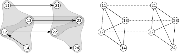
Figure 1: The prime hypergraph $H$ (left-hand side) with arc set $E(H)=\{{e_{1}=(\{11,12,13\},\{12,13,14\})},KA:{e_{2}=(\{21,22,23\},\{22,23,24\})},e_{3}=(\{14\},\{12\}),e_{4}=(\{11\},\{21\}),{e_{5}=(\{12\},\{22\})},{e_{6}=(\{13,23\},\{13,23\})},{e_{7}=(\{14\},\{24\})},{e_{8}=(\{13\},\{23\})}\}$ admits a non-trivial prime factorization of its 2-section $[H]_{2}$ (right-hand side) into $K_{4}\Box K_{2}$. The vertices of $H$ are labeled w.r.t. its pre-coordinatization given by the coordinatization of $[H]_{2}$. For the first arc $e_{4}$ of the lexicographic ordered arc set $E_{\textrm{lex}}=\{e_{4},e_{1},e_{5},e_{8},e_{6},e_{3},e_{7},e_{2}\}$ we can observe that the increment $\textrm{inc}(e_{4},2)=((\{12\},\{22\})=e_{5}\in E_{\textrm{lex}}$. Analogously, $\textrm{inc}(e_{1},1)=e_{2}$, $\textrm{inc}(e_{5},2)=e_{8}$, and $\textrm{inc}(e_{8},2)=e_{7}$ are all contained in $E_{\textrm{lex}}$. However, when we arrive at the hyperedge $e_{6}$ we obtain that $\textrm{inc}(e_{6},2)=(\{14,24\},\{14,24\})$ is not an arc of $E_{\textrm{lex}}$. Hence, applying Algorithm 1 would lead to an edge $12$ in $G_{\textrm{aux}}$, resulting in a connected auxiliary graph and, $H$ would be determined as prime. A second example for an arc $e\in E_{\textrm{lex}}$ with $\textrm{inc}(e,i)\notin E_{\textrm{lex}}$ is the edge $e=e_{7}$.

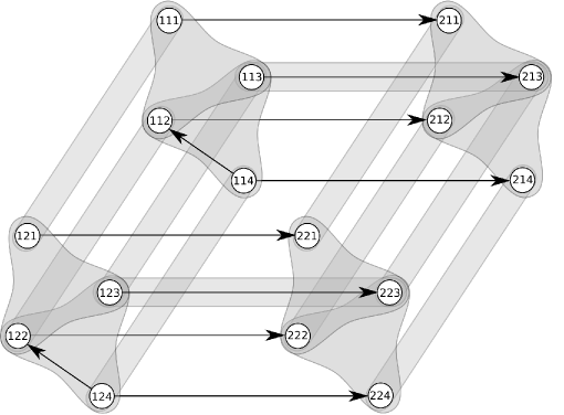
Figure 2: The non-prime hypergraph $H=H_{1}\Box H_{2}$ is the product of the directed prime hypergraph $H_{1}$ in Fig. 1 and an undirected hypergraph $H_{2}$ with two vertices and one hyperedge. The vertices of $H$ are labeled w.r.t. its pre-coordinatization given by the coordinatization of $[H]_{2}$. The auxiliary graph $G_{\textrm{aux}}$ is initialized as the graph with three vertices and empty edge-set in Algorithm 1. While the increment $\textrm{inc}(e,2)=\{(123,223),(123,223)\}$ of the arc $e=\{(113,213),(113,213)\}$ is still contained in $E_{\textrm{lex}}$, the increment $\textrm{inc}(e,3)=\{(124,224),(124,224)\}$ is not. Hence, the edge $13$ is added to $G_{\textrm{aux}}$. Since the increments of all hyperedges of the form $\{(i1j,i2j),(i1j,i2j)\}$ are contained in $E_{\textrm{lex}}$, no further edges will be added to $G_{\textrm{aux}}$. Hence, the sub-hypergraph induced by vertices with identical 2nd coordinate, i.e., the $\{1,3\}$-layers, constitute the copies the prime factor $H_{1}$, while the sub-hypergraphs induced by vertices with identical 1st and 3rd coordinate, i.e, the $2$-layers, are copies of the prime factor $H_{2}$.

3.2 Correctness

We are now in the position to prove the correctness of the algorithm PFD_of_Di-Hypergraphs, summarized in the following theorem.

Theorem 3.12.

Algorithm 1 is sound and complete.

Proof.

Given a hypergraph $H=(V,E)$. We start with a preprocessing and call in Algorithm 1 the Algorithm 2. Here, the PFD of $[H]_{2}=\Box_{i=1}^{k}G_{i}$ and the respective coordinatization $\Upsilon$ of $[H]_{2}$ is computed. This coordinatization $\Upsilon$ is by definition a pre-coordinatization of $H$. Since $[H]_{2}$ is an undirected graph, it is allowed to apply the algorithm of Imrich and Peterin [21]. Finally, the vertices, the vertices within the arcs and the arcs are ordered in lexicographic order. The latter task is not important for the correctness of the algorithm, but for the time-complexity that we will consider later on.

We are now in Line 3 of Algorithm 1. By construction of $\Upsilon$ and Lemma 2.3, the pre-coordinatization $\Upsilon$ is at least as fine as the coordinatization of $H$ w.r.t. its PFD. By Lemma 2.10 it suffices to find a suitable partition of $I=\{1,\dots,k\}$. To this end, we initialize in the auxiliary graph $G_{\textrm{aux}}$ where each vertex $i$ represents an element of $I$. The edge set is left empty. We might later add edges in order trace back which equivalence classes have to be combined, i.e., all vertices within one connected components of $G_{\textrm{aux}}$ will then be in one class of the respective partition of $I$.

Now consider the for-loop in Line 4-11. For each $e\in E_{\textrm{lex}}$ we check in which coordinates the vertices in $V(e)$ differ. Since $\Upsilon$ is a pre-coordinatization and by Lemma 2.7, this is exactly one coordinate for each hyperarc. Let $e\in E_{\textrm{lex}}$ be a chosen arc and assume that all vertices in $V(e)$ differ in the $j$-th coordinate. Now, it is checked if for arc $e$ its “copies” are contained in each $G_{j}^{w}$-layer where $w\in inc(V(e),i)$. If for some arc $e\in E_{\textrm{lex}}$ we observe that there is no hyperedge $\textrm{inc}(e,i)=(\textrm{inc}(t(e),i),\textrm{inc}(h(e),i)\in E_{\textrm{lex}}$ then there is no “copy” of $e$ in some $j$-pre-layer through $w$ with $w\in inc(V(e),i)$. In this case we add the edge $ij$ to $G_{\textrm{aux}}$ if not already set. The latter tasks are repeated for all hyperarcs $e\in E_{\textrm{lex}}$.

Finally, in Line 12 the Algorithm 3 is called. The task of this subroutine is to combine the pre-coordinates and thus, the pre-layers in order to determine the layers of the final prime-factors of $H$. Let $I_{1},\dots,I_{r}$ be the connected components of $G_{\textrm{aux}}$. Clearly, $\Pi=\{I_{1},\dots,I_{r}\}$ is a partition of $I$. Let each $I_{j}$ having $l_{j}$ elements. Lemma 2.10 and Remark 2 imply that $\widehat{\Upsilon}\colon V(H)\to\mathop{\hbox{\Large{$\times$}}}_{l=1}^{r}\{1,\dots,l_{r}\}$ is a pre-coordinatization of $H$. It remains to show that

1. $\widehat{\Upsilon}$ is a coordinatization and

2. $\widehat{\Upsilon}$ is at least as fine as the coordinatization given by the PFD of $H$.

Claim (1.): By construction, all $e\in E_{\textrm{lex}}$ where the vertices differ in the $i$-th coordinate w.r.t. $\Upsilon$ are now contained in some $I_{s}$-layer where $i\in I_{s}\in\Pi$. Moreover, for all $e$ in some $I_{s}$-layer the increments $\textrm{inc}(e,j)$ with $j\neq i$ and $j\notin I_{s}$ must be contained in $H$, as otherwise we would have added the edge $ij$ to $G_{\textrm{aux}}$ and hence, $j\in I_{s}$. As the latter is true for all $I_{s}$-layers contained in $\Pi$ we can apply Lemma 2.11 and conclude that $\widehat{\Upsilon}$ is a coordinatization of $H$.

Claim (2.): Given the pre-coordinatization $\Upsilon$ of $H$. By construction of $\Upsilon$ and Lemma 2.3, $\Upsilon$ is at least as fine as the coordinatization of $H$ w.r.t. its PFD. Thus, there is a partition $\Pi^{\prime}=\{I^{\prime}_{1},\dots,I^{\prime}_{t}\}$ of $I$ w.r.t. the PFD of $H$. It remains to show that if there are two indices $i,j\in I_{s}\in\Pi$, then $i,j$ are also contained in the same class of $\Pi^{\prime}$. If $i,j\in I_{s}\in\Pi$ then they are in same connected component $C_{s}$ of $G_{\textrm{aux}}$. Hence, it suffices to consider pairs $i,j\in I_{s}\in\Pi$ that are connected by an edge. Assume, for contradiction that $i,j$ are in different classes of $\Pi^{\prime}$. W.l.o.g. let $i\in I^{\prime}_{1}$ and $j\in I^{\prime}_{2}$. Moreover, let $H=H_{I^{\prime}_{1}}\Box H_{\cup_{l\geq 2}I^{\prime}_{l}}$ Hence, for all $l\in I^{\prime}_{1}$ and thus, in particular for $l=i$ it holds that for all arcs $e$ in some $I^{\prime}_{2}$-layer there is an arc $(\textrm{inc}(t(e),i),\textrm{inc}(h(e),i)\in E_{\textrm{lex}}$. The same holds with the role of $i$ and $j$ switched. However, in this case we would not add the edge $ij$ to $G_{\textrm{aux}}$, a contradiction.

To finish the PFD-computation we have to compute $\widehat{\Upsilon}$. To this end, we compute the 2-section $[H]_{2}$ with edges $xy$ colored with color $j$ whenever $x$ and $y$ are contained in some edge $e$ that is contained in some $j$-layer of $H$. Lemma 2.3 implies that $\widehat{\Upsilon}$ is also a coordinatization of $[H]_{2}$ and hence, all edges with same color $j$ in $[H]_{2}$ are contained in the same equivalence class of $R_{\widehat{\Upsilon}}([H]_{2})$. In other words, $(e,f)\in R_{\widehat{\Upsilon}}(H)$ if and only if $(xy,uv)\in R_{\widehat{\Upsilon}}([H]_{2})$ for all distinct $x,y\in V(e)$ and distinct $u,v\in V(f)$. By construction, $R_{\widehat{\Upsilon}}([H]_{2})$ is a a product relation of $[H]_{2}$, and thus we can apply again a method proposed the by Imrich and Peterin (cf. Theorem 5.1. in [21]), in order to obtain the desired coordinates and hence, $\widehat{\Upsilon}$. ∎

3.3 Time Complexity

In order to prove the time-complexity results, we first give the following lemma.

Lemma 3.13.

Let $H$ be a hypergraph, let $[H]_{2}=\Box_{i=1}^{k}H_{i}$ be a factorization of its $2$-section into $k$ factors, and let $m$ and $n$ be the number of arcs and vertices of $H$, respectively. Then for any $l\in\mathbb{N}_{0}$ it holds that $k^{l}\log m=O(n)$.

Proof.

If $m_{i}$ and $n_{i}$ are the numbers of arcs and vertices of the factors then $m_{i}\leq(2^{n_{i}})^{2}$, since we have to consider tail and head independently. Let $N$ be the maximum number of vertices of a factor. Then we have

$$m=\sum_{i=1}^{k}m_{i}\prod_{\begin{subarray}{c}j=1\\ j\neq i\end{subarray}}^{k}n_{j}\leq\sum_{i=1}^{k}2^{n_{i}}\prod_{j=1}^{k}n_{j}\leq k\cdot 2^{N}\prod_{j=1}^{k}n_{j}.$$

Taking logarithms on both sides of the inequality gives

$$\log m\leq\log k+N+\sum_{j=1}^{k}\log(n_{i})\leq k+N+k\cdot N\leq c\cdot k\cdot N$$

for some suitable constant $c$.

On the other hand by bounding the size of every factor except the biggest one from below by $2$ we get $n=\prod_{i=1}^{k}n_{i}\geq N\cdot 2^{k-1}$. Clearly, $N\cdot 2^{k-1}\geq c^{\prime}\cdot N\cdot k^{l}$ for some suitable constant $c^{\prime}$ depending on $l$. Together with the estimate for $\log m$ this proves the lemma. ∎

The next two lemmas are concerned with the time-complexity of the subroutines Preprocessing and Combine.

Lemma 3.14.

Let $H=(V,E)$ be a connected hypergraph with $|V|=n$, $|E|=m$ and rank $r$. Then Algorithm 2 performs in $O(r^{2}mn)$ time. If we assume that $H$ has bounded rank, then Algorithm 2 has time-complexity $O(m\log^{2}(n))$.

Proof.

In Line 2, the first task is the computation of the 2-section $[H]_{2}$. To this end, we initialize an adjacency list $N[1],\dots,N[n]$ with empty entries, which can be done in $O(n)$ time. We add for each arc $e\in E$ and each pair $\{i,j\}\in\binom{V(e)}{2}$ the vertex $i$ to $N[j]$ and $j$ to $N[i]$, if these vertices are not already contained in the respective adjacency lists. Hence, we must check whether $i\in N[j]$ or not. To this end, assume that $N[j]$ is already ordered. Hence we need $O(\log(n))$ comparisons to verify if $i\in N[j]$. If this is not the case, the vertex $i$ is added to $N[j]$ on the respective position so that $N[j]$ stays sorted. Analogously, we add $j$ to $N[i]$, whenever $j$ is not contained in $N[i]$. As for each arc $e\in E$ there are at most $\binom{r}{2}=O(r^{2})$ pairs $\{i,j\}$ and for each such pair we have $O(\log(n))$ comparisons we end in a time-complexity of $O(n+mr^{2}\log(n))$ to create the adjacency list $N[1],\dots,N[n]$. These lists serve than as input for the algorithm of Imrich and Peterin which computes the PFD of the 2-section in $O(|E([H]_{2})|+n)$ time. Since $[H]_{2}$ is connected and thus, $[H]_{2}$ has at least $|V|-1$ edges, the PFD algorithm runs in fact in $O(|E([H]_{2}|)=O(mr^{2})$ time. Hence, the total time complexity of Line 2 of Algorithm 2 is $O(n+mr^{2}\log(n)+mr^{2})=O(mr^{2}\log(n))$.

In what follows, let $k$ be the number of factors of $[H_{2}]$ and let each $v\in V$ be identified with its respective (pre-) coordinate vector $(v_{1},\dots,v_{k})$ computed by the Imrich-Peterin-Algorithm. Note, $k$ is bounded by $\log(n)$.

In Line 3, the list $V$ of vertices is reordered in lexicographic order w.r.t. the vertex coordinates, i.e., $v<w$ if there is some $i\in\{1,\dots,k\}$ with $v_{j}\leq w_{j}$ for all $j\in\{1,\dots,i-1\}$ and $v_{i}<w_{i}$. This task can be done in $O(n\log(n)k)=O(n\log^{2}(n))$. Since $mr\geq n$ we obtain that $O(n\log^{2}(n))=O(mr\log^{2}(n))$. This new ordered vertex list is called $V_{\textrm{lex}}$.

We are now concerned with the for-loop in Line 4. For each hyperedge $e\in E$ we reorder the vertices of its head and tail w.r.t. to the order of the vertices in $V_{\textrm{lex}}$. Each hyperedge contains at most $r$ vertices and hence, this task can be done in $O(r\log(r))$ time. Therefore, the entire for-loop (Line 4 - 6) takes $O(mr\log(r))$ time.

Finally, the arcs are reordered w.r.t. the lexicographic ordered sets $t(e)$ and $h(e)$. We say $e<f$ if $t(e)<t(f)$ or $t(e)=t(f)$ and $h(e)<h(f)$, whereby the tails, resp., heads are compared w.r.t. the lexicographic order of their vertices. To determine if $t(e)<t(f)$ or $h(e)<h(f)$ for some arcs $e,f\in E$, the at most $2r$ pairs of vertices must be compared, whereby the comparison of each such pair can be done in $O(1)$ time, since the vertices are already ordered in the tails and heads. The reordering of the arcs need than $O(m\log(m))$ comparisons, where each comparison can be done in $O(r)$ time, by the preceding arguments. Hence, the creation of $E_{\textrm{lex}}$ takes $O(rm\log(m))$ time. By Lemma 3.13 this is $O(rmn)$. Moreover, if we assume that the rank $r$ is bounded, then $m\leq\sum_{i=1}^{r}\binom{n}{r}\leq rn^{r}=O(n^{r})$. Hence $O(\log(m))=O(\log(n^{r}))=O(r\log(n))=O(\log(n))$. In this case the time complexity for determining $E_{\textrm{lex}}$ is $O(m\log(m))=O(m\log(n))$.

Taken together the latter arguments, we end in overall time complexity for Algorithm 2 of $O(r^{2}mn)$ and if the rank $r$ is bounded with $O(m\log^{2}(n))$. ∎

Lemma 3.15.

Let $H=(V,E)$ be a connected hypergraph with $|V|=n$, $|E|=m$ and rank $r$. Moreover, assume that the graph $G_{\textrm{aux}}$ has $k$ vertices and $m^{\prime}$ edge with $k\leq\log(n)$. Then Algorithm 3 preforms in $O(mnr^{2})$ time. If we assume that $H$ has bounded rank, then Algorithm 3 has time-complexity $O(m\log^{2}(n))$.

Proof.

Determining the connected components of $G_{\textrm{aux}}$ in Line 2 can be done in $O(k+m^{\prime})=O(\log(n)+\log^{2}(n))$ time by application of the classical breadth-first search. While doing this, we will in addition record in $O(1)$ time for each vertex in which connected component it is contained. Let $I_{1},\dots,I_{l}$ be the connected components of $G_{\textrm{aux}}$.

For each of the $m$ arcs we have to find the indices where the vertices of the particular arc differs. To this end, it suffices to take any two vertices $x$ and $y$ of $V(e)$ and to compare their $k$ coordinates which takes $O(k)$ time. Let $j$ be the coordinate where the two vertices differ. We need to check in which of the connected components $I_{s}$ the vertex is contained in, which can be done in $O(1)$ time, since we have already recorded for each vertex of $G_{\textrm{aux}}$, in which component it is contained in. Now, the color for each arc can be recorded in $O(1)$ time. Hence, the for-loop (Line 3-7) has overall-time complexity $O(mk)=O(m\log(n))$.

To compute the 2-section in Line 8 with colored edges we initialize an extended adjacency list $N[1],\dots,N[n]$ where whenever we add some $i\in N[j]$ we also record the respective unique color of $ij$ as a 2nd parameter. Recording this parameter can be done in $O(1)$ time, as for each arc $e\in E$ it is known which color it has. Hence, we can argue analogously as in the proof of Lemma 3.14, and state that the 2-section with additionally colored edges can be computed in $O(n+mr^{2}\log(n))$ time.

Finally, the vertex-coordinates in $[H]_{2}$ can be computed in $O(m^{\prime})=O(mr^{2})$ time, see Theorem 5.1. in [21].

Hence the overall-time complexity of Algorithm 3 is $O(\log^{2}(n)+m\log(n)+n+mr^{2}\log(n)+mr^{2})=O(n+m\log^{2}(n)r^{2})$. Since $mr\geq n$ and $\log^{2}(n)=O(n)$, the latter can be expressed as $O(mnr^{2})$. If we assume in addition that the rank $r$ is bounded we get $O(n+m\log^{2}(n)r^{2})=O(mr+m\log^{2}(n)r^{2})=O(m\log^{2}(n))$. ∎

We are now in the position to determine the time-complexity of algorithm PFD_of_Di-Hypergraphs.

Theorem 3.16.

Let $H=(V,E)$ be a connected hypergraph with $|V|=n$, $|E|=m$ and rank $r$. Then Algorithm 1 computes the PFD of $H$ in $O(mnr^{2})$ time. If the rank $r$ is bounded the time-complexity of Algorithm 1 is $O(m\log^{2}(n))$.

Proof.

We suppose both the vertices and the hyperarcs of $H$ implemented as integers and $E$ implemented as an $m\times 2$ array, where each entry $E[e,i]$ contains the list of vertices in $t(e)$ if $i=1$ and $h(e)$ if $i=2$. In Line 2 we call Preprocessing($H$) which takes $O(r^{2}mn)$ time and if $r$ is bounded $O(m\log^{2}(n))$ time (Lemma 3.14).

In what follows, let $k\leq\log(n)$ be the number of factors of $[H_{2}]$ and assume that each $v\in V$ is identified with its respective (pre-)coordinate vector $(v_{1},\dots,v_{k})$.

In Line 3 the auxiliary graph is be initialized. In particular, we initialize $G_{\textrm{aux}}$ as adjacency list, i.e., we create empty lists $N[1],\dots,N[k]$ which can be done in $O(k)$ time.

We are now concerned with the for-loop in Line 4 - 11. For each of the $m$ arcs we have to find the indices where the vertices of the particular arc differs. To this end, any two vertices $x$ and $y$ of $V(e)$ are chosen and their $k$ coordinates are compared, which takes $O(k)$ time. The nested for-loop (Line 6 - 10) is executed for all coordinates $i$ where the vertices of arc $e$ are identical and it is checked whether $\textrm{inc}(e,i)=(\textrm{inc}(t(e),i),\textrm{inc}(h(e),i)$ is contained in $E_{\textrm{lex}}$ or not. The increment $(\textrm{inc}(t(e),i),\textrm{inc}(h(e),i)$ can be computed in $O(r)$ time. Note, the vertices within $\textrm{inc}(t(e),i)$ and $\textrm{inc}(h(e),i)$ are still lexicographically ordered as only vertex-coordinates are incremented that have been identical for the vertices within the arc and thus,their $i$-th positions are all still equal after the computation of $\textrm{inc}(e,i)$. We now check whether $(\textrm{inc}(t(e),i),\textrm{inc}(h(e),i)\notin E_{\textrm{lex}}$. Since $E_{\textrm{lex}}$ is already ordered, binary search finds the corresponding arc using at most $O(\log(m))$ comparisons of arcs and since head and tail of each arc are in lexicographic order comparing two arcs takes $O(r)$ time. Therefore, the if-condition in Line 7 takes $O(r+r\log(m))=O(r\log(m))$ time. In case, $(\textrm{inc}(t(e),i),\textrm{inc}(h(e),i)\notin E_{\textrm{lex}}$ we have to add a respective edge $ij$ in $G_{\textrm{aux}}$, if not already set. Hence, to check whether $ij$ exists in $G_{\textrm{aux}}$, we need to validate if $i\in N[j]$. To this end, assume that $N[j]$ is already ordered. Hence we need $O(\log(k))$ comparisons to verify if $i\in N[j]$. If this is not the case $i$ is added to $N[j]$ on the respective position so that $N[j]$ stays sorted. Similarly, $j$ is added to $N[i]$ whenever $i\not\in N[j]$. Hence the nested for-loop in (Line 6 - 10) has time complexity $O(k(r\log(m)+\log(k)))=O(kr\log(m))$, since the number of arcs $m$ is at least as big as the number (non-trivial) factors $k$. Take together the latter arguments, the entire for-loop in Line 4 - 11 has time-complexity $O(m(k+kr\log(m)))=O(mkr\log(m))$. By Lemma 3.13 this is $O(mnr)$. Moreover, if we assume that the rank $r$ is bounded, then $m\leq n^{r}$ and hence, $O(\log(m))=O(\log(n^{r}))=O(r\log(n))=O(\log(n))$ In this case, the time complexity of Line 4 - 11 is $O(mk\log(m))=O(mk\log(n))=O(m\log^{2}(n))$.

Finally, we use Algorithm 3 which performs in $O(mnr^{2})$ time and if the rank $r$ is bounded it has time-complexity $O(m\log^{2}(n))$ (Lemma 3.15).

To summarize, each step of Algorithm 1 can be performed in $O(mnr^{2})$ time and if the rank $r$ is bounded the time-complexity is $O(m\log^{2}(n))$. ∎

References

- Aurenhammer et al. [1992] Aurenhammer, F., Hagauer, J., Imrich, W., 1992. Cartesian graph factorization at logarithmic cost per edge. Comput. Complexity 2, 331–349.
- Berge [1989] Berge, C., 1989. Hypergraphs: Combinatorics of finite sets. volume 45. North-Holland, Amsterdam.
- Black [2015] Black, T., 2015. Monotone properties of k-uniform hypergraphs are weakly evasive, in: Proceedings of the 2015 Conference on Innovations in Theoretical Computer Science, ACM, New York, NY, USA. pp. 383–391.
- Brešar [2004] Brešar, B., 2004. On subgraphs of Cartesian product graphs and S-primeness. Discr. Math. 282, 43–52.
- Bretto [2006] Bretto, A., 2006. Hypergraphs and the Helly property. Ars Comb. 78, 23–32.
- Bretto [2013] Bretto, A., 2013. Applications of hypergraph theory: A brief overview, in: Hypergraph Theory. Springer International Publishing. Mathematical Engineering, pp. 111–116.
- Bretto et al. [2009] Bretto, A., Silvestre, Y., Vallée, T., 2009. Cartesian product of hypergraphs: properties and algorithms, in: 4th Athens Colloquium on Algorithms and Complexity (ACAC 2009), pp. 22–28.
- Bretto et al. [2013] Bretto, A., Silvestre, Y., Vallée, T., 2013. Factorization of products of hypergraphs: Structure and algorithms. Theoretical Computer Science 475, 47 – 58.
- Crespelle et al. [2013] Crespelle, C., Thierry, E., Lambert, T., 2013. A linear-time algorithm for computing the prime decomposition of a directed graph with regard to the Cartesian product, in: Du, D.Z., Zhang, G. (Eds.), Computing and Combinatorics. Springer Berlin Heidelberg. volume 7936 of Lecture Notes in Computer Science, pp. 469–480.
- Dörfler [1979] Dörfler, W., 1979. Multiple Covers of Hypergraphs. Annals of the New York Academy of Sciences 319, 169–176.
- Feder [1992] Feder, T., 1992. Product graph representations. J. Graph Theory 16, 467–488.
- Feigenbaum [1986] Feigenbaum, J., 1986. Directed Cartesian-product graphs have unique factorizations that can be computed in polynomial time. Discrete Appl. Math. 15, 105 – 110.
- Feigenbaum et al. [1985] Feigenbaum, J., Hershberger, J., Schäffer, A., 1985. A polynomial time algorithm for finding the prime factors of Cartesian-product graphs. Discrete Appl. Math. 12, 123–138.
- Hammack et al. [2011] Hammack, R., Imrich, W., Klavžar, S., 2011. Handbook of Product Graphs. Discrete Mathematics and its Applications. 2nd ed., CRC Press.
- Hellmuth [2013] Hellmuth, M., 2013. On the complexity of recognizing S-composite and S-prime graphs. Discrete Applied Mathematics 161, 1006 – 1013.
- Hellmuth et al. [2014] Hellmuth, M., Noll, M., Ostermeier, L., 2014. Strong products of hypergraphs: Unique prime factorization theorems and algorithms. Discrete Applied Mathematics 171, 60 – 71.
- Hellmuth et al. [2012a] Hellmuth, M., Ostermeier, L., Stadler, P., 2012a. Diagonalized Cartesian products of S-prime graphs are S-prime. Discrete Math. 312, 74 – 80. Algebraic Graph Theory - A Volume Dedicated to Gert Sabidussi on the Occasion of His 80th Birthday.
- Hellmuth et al. [2012b] Hellmuth, M., Ostermeier, L., Stadler, P.F., 2012b. A survey on hypergraph products. Math. Comput. Sci. 6, 1–32.
- Imrich [1967] Imrich, W., 1967. Kartesisches Produkt von Mengensystemen und Graphen. Studia Sci. Math. Hungar. 2, 285 – 290.
- Imrich [1971] Imrich, W., 1971. Über das schwache Kartesische Produkt von Graphen. Journal of Combinatorial Theory 11, 1–16.
- Imrich and Peterin [2007] Imrich, W., Peterin, I., 2007. Recognizing Cartesian products in linear time. Discrete Math. 307, 472–483.
- Kaveh and Alinejad [2012] Kaveh, A., Alinejad, B., 2012. Hypergraph products for structural mechanics, in: Topping, B. (Ed.), Proceedings of the Eleventh International Conference on Computational Structures Technology, Civil-Comp Press, Stirlingshire, UK. doi:10.4203/ccp.99.266. paper 266.
- Kaveh and Alinejad [2015] Kaveh, A., Alinejad, B., 2015. Hypergraph products for structural mechanics. Advances in Engineering Software 80, 72 – 81. Civil-Comp.
- Klavžar et al. [2002] Klavžar, S., Lipovec, A., Petkovšek, M., 2002. On subgraphs of Cartesian product graphs. Discr. Math. 244, 223–230.
- Ostermeier et al. [2012] Ostermeier, L., Hellmuth, M., Stadler, P.F., 2012. The Cartesian product of hypergraphs. Journal of Graph Theory 70, 180–196.
- Sabidussi [1960] Sabidussi, G., 1960. Graph Multiplication. Mathematische Zeitschrift 72, 446–457.
- Shapiro [1953] Shapiro, H., 1953. The embedding of graphs in cubes and the design of sequential relay circuits. Bell Telephone Laboratories Memorandum Unpublished.
- Sonntag [1989] Sonntag, M., 1989. Hamiltonian properties of the Cartesian sum of hypergraphs. J. Inf. Process. Cybern. 25, 87–100.
- Szamkołowisz [1962] Szamkołowisz, L., 1962. Remarks on the Cartesian product of two graphs. Colloq. Math. 9, 43–47.
- Vizing [1963] Vizing, V.G., 1963. The Cartesian product of graphs. Vyčisl. Sistemy No. 9, 30–43.
- Winkler [1987] Winkler, P., 1987. Factoring a graph in polynomial time. European J. Combin. 8, 209–212.
- Zhu [1992] Zhu, X., 1992. On the chromatic number of the product of hypergraphs. Ars Comb. 34, 25–31.