State of the art for ab initio vs empirical potentials for predicting 6e^- excited state molecular energies: Application to Li${}_{2}\left(b,1^{3}\Pi_{u}\right)$

Abstract

We build the first analytic empirical potential for the most deeply bound Li₂ state: $b\left(1^{3}\Pi_{u}\right)$. Our potential is based on experimental energy transitions covering $v=0-34$, and very high precision theoretical long-range constants. It provides high accuracy predictions up to $v=100$ which pave the way for high-precision long-range measurements, and hopefully an eventual resolution of the age old discrepancy between experiment and theory for the Li$\left(2^{2}S\right)+\mbox{Li}\left(2^{2}P\right)$ $C_{3}$ value. State of the art ab initio calculations predict vibrational energy spacings that are all in at most 0.8 cm^-1 disagreement with the empirical potential.

There is currently a rather large discrepancy between the best atomic 3e^- ab initio calculation Tang et al. (2010a), and the most current empirical value Gunton et al. (2013a); Le Roy et al. (2009), for the leading long-range Li$(2^{2}S)-\mbox{Li$(2^{2}P)$}$ interaction constant ($C_{3}$), despite the latter being the most precise experimentally determined oscillator strength for any system, by an order of magnitude Tang et al. (2011). $\mbox{Li}_{2}(b,1^{3}\Pi_{u})$ is one of the molecular states that dissociates to Li$(2^{2}S)+\mbox{Li$(2^{2}P)$}$, and therefore its long-range potential has this $C_{3}$ interaction constant. This “$b$-state” is also the deepest Li₂ potential, and out of the five lowest Li₂ states, the $b$-state is the only one for which an analytic empirical potential has never been made.

Since the highest 2000 cm^-1 worth of vibrational levels of the $b$-state still have not been observed, and part of this region is now accessible by current ultra-high precision PA (photoassociation) technology Gunton et al. (2013a); Semczuk et al. (2013), an analytic potential would be very useful for making predictions to assist in observing the missing levels. The $b$-state also mixes strongly with the $A(1^{1}\Sigma_{u})$-state , which has by far the most precisely determined excited molecular state potential in all of chemistry, yet still has a rather large gap of missing data in the middle of its energy range Gunton et al. (2013a); Le Roy et al. (2009).

Finally, the $b(1^{3}\Pi_{u})$-state has been a key doorway to the triplet manifold, and was directly involved in the measurements for a vast number of other triplet states such as $2^{3}\Delta_{g}$ Yi et al. (2001), $3^{3}\Pi_{g}$ Yiannopoulou et al. (1995a), $3^{3}\Sigma_{g}^{+}$ Yiannopoulou et al. (1995a); Li et al. (2007); Xie and Field (1986), $2^{3}\Sigma_{g}^{+}$ Yiannopoulou et al. (1995a); Lazarov et al. (2001), $2^{3}\Pi_{g}$ Xie and Field (1986); Yiannopoulou et al. (1995a); Russier et al. (1997); Li et al. (2007), $1^{3}\Delta_{g}$ Xie and Field (1986); Linton et al. (1992); Yiannopoulou et al. (1995b); Weyh et al. (1996a); Russier et al. (1997); Li et al. (2007), $1^{3}\Sigma_{g}^{-}$, and other undetermined ${}^{3}\Lambda$ states Rai et al. (1985); Li et al. (1996). Some of these more highly excited triplet states (namely $3^{3}\Sigma_{g}^{+},$ $2^{3}\Sigma_{g}^{+},$ $2^{3}\Pi_{g},$ and $1^{3}\Delta_{g}$) are so thoroughly covered by these spectroscopic measurements, that global empirical potentials can be built for them too. For this, an analytic potential for the $b$-state would be used as a base.

In this work we will build analytic empirical potentials for the $b$-states of all stable homonuclear isotopologues of Li₂. Previous work has shown that analytic empirical potentials for the $c(1^{3}\Sigma_{g})$-state were able to predict energies correctly to about 1 cm^-1, in the middle of a gap of $>5000$ cm^-1 where data were unavailable Dattani and Le Roy (2011a); Semczuk et al. (2013), and this was much better agreement than was obtained with the most sophisticated Li₂ ab initio calculations of the time Halls et al. (2001).

It was recently shown that the best ground-state rotationless ab initio potentials for the 5e^- molecules BeH, BeD, and BeT, were able to predict vibrational energy spacings to within 1 cm^-1 for all measured energy levels except one. The $b$-state of Li₂ might be expected to be more challenging ab initio because it (1) is an excited state, (2) has one more e^-, and (3) involves many more vibrational energies. We will therefore compare our analytic empirical potentials for the $b$-state of ^6,6Li₂ and ^7,7Li₂ with the most state-of-the-art ab initio calculations, which were published recently in Musial and Kucharski (2014).

Table 1 summarizes all experiments we could find which provided information on rovibrational levels of the $b$-state . Unfortunately attempts to recover the data from Engelke and Hage (1983); Rai et al. (1985); Xie and Field (1986); Schmidt et al. (1988); Weyh et al. (1996b) were unsuccessful, but we were still able to include all data from the other experiments in our study. Furthermore, it is noted that the $b$-state was also involved in various other studies Yiannopoulou et al. (1995a, c); Li and Lyyra (1999); Yi et al. (2001); Li et al. (2007) but these just made use of rovibrational levels that were already determined in the studies listed in Table 1, in order to access levels of other electronic states.

Table 1: Summary of experiments involving Li${}_{2}(b,1^{3}\Pi_{u})$

 

Isotopes	Year	Type	States Involved	Unc. (cm-1)	$v$	# Data	Included in dataset	Source
7,7Li2	1985	LIF	$A(1^{1}\Sigma_{u}^{+}),b(1^{3}\Pi_{u})$	$a$	$8-25$	100s		Preuss & Baumgartner Preuss and Baumgartner (1985)
	1985	OODR	$(5d\delta^{3}\Delta_{g})\rightarrow b(1^{3}\Pi_{u})$	1	$0$	100s	-	Rai et al Rai et al. (1985)
	1992	PFOODR	$A(1^{1}\Sigma_{u}^{+}),b(1^{3}\Pi_{u})$	?	$19$	3	-	Li et al. Li et al. (1992)
	1996	cw PFOODR	$({}^{3}\Lambda_{g})\rightarrow b(1^{3}\Pi_{u})$	?	$0,1,4$	?	-	Li et al.Li et al. (1996)
	1996	CIF	$(1^{3}\Delta_{g})\rightarrow b(1^{3}\Pi_{u})$	?	$0-11$	?	-	Weyh et al.Weyh et al. (1996b)
	1997	PFOODR	$(2^{3}\Pi_{g})\rightarrow b(1^{3}\Pi_{u})$	0.005	$1-27$	178	$\checkmark$	Russier et al Russier et al. (1997)
	1997	PFOODR	$(1^{3}\Delta_{g})\rightarrow b(1^{3}\Pi_{u})$	0.005	$1-25$	234	$\checkmark$	Russier et al Russier et al. (1997)
	1997	CIF	$(1^{3}\Delta_{g})\rightarrow b(1^{3}\Pi_{u})$	0.005	$0-7$	314	$\checkmark$	Russier et al Russier et al. (1997)
	2001	cw PFOODR	$A(1^{1}\Sigma_{u}^{+}),b(1^{3}\Pi_{u})$	?	$15,22$	2	-	Lazarov & Lyyra Lazarov et al. (2001)
7,6Li2	1985	LIF	$A(1^{1}\Sigma_{u}^{+}),b(1^{3}\Pi_{u})$	$a$	$8-20$	100s		Preuss & BaumgartnerPreuss and Baumgartner (1985)
6,6Li2	1983	CIF	$(3^{3}\Delta_{g})\rightarrow b(1^{3}\Pi_{u})$	$0.3$	$0-10$	240	-	Engelke & Hage
	1985	LIF	$A(1^{1}\Sigma_{u}^{+}),b(1^{3}\Pi_{u})$	$a$	$8-18$	100s		Preuss & BaumgartnerPreuss and Baumgartner (1985)
	1985		$A(1^{1}\Sigma_{u}^{+}),b(1^{3}\Pi_{u})$	?	$9,15$	2	-	Xie & Field Xie and Field (1985a, b)
	1986	PFOODR	$(2^{3}\Pi_{g})\rightarrow b(1^{3}\Pi_{u})$	$0.5$	$0-17$	~170	32 lines recovered	Xie & Field Xie and Field (1986)
	1986	PFOODR	$(1^{3}\Delta_{g})\rightarrow b(1^{3}\Pi_{u})$	$0.02-0.13$	$0-11$	?		Rice, Xie & Field Rice et al. (1986); Rice, Steven F. and Field (1986)
	1988	CIF	$(1^{3}\Delta_{g})\rightarrow b(1^{3}\Pi_{u})$	$0.2$	$0-11$	~200	-	Schmidt et al. Schmidt et al. (1988)
	1992	CIF	$(1^{3}\Delta_{g})\leftrightarrow b(1^{3}\Pi_{u})$	$0.003-0.07$	$0-9$	599	$\checkmark$	Linton et al. Linton et al. (1992)
TOTAL				$0.003-1$	$0-27$	?	1357	Linton et al. (1992)Russier et al. (1997)

 

^aThe measurements were on $v$-levels of the $A$-state, and information about the $b$-state $v$-levels that perturbed those $A$-state levels was inferred indirectly.

I Hamiltonian

The rovibrational energy levels and wavefunctions for isotopologue $\alpha$ with reduced mass $\mu_{\alpha}$ are treated as the eigenvalues and eigenfunctions in the effective radial Schroedinger equation:

$$\left(-\frac{\hbar}{2\mu_{\alpha}}\frac{{\rm d}^{2}}{{\rm d}r^{2}}+V_{{\rm\alpha}}(r)+\frac{\hbar N(N+1)}{2\mu_{\alpha}r^{2}}\left(1+g_{{\rm\alpha}}(r)\right)\right)\psi_{v,N}(r)=E_{v,N}(r)\psi_{v,N}\,.$$ (1)

Here $V_{\alpha}(r)$ and $g_{\alpha}(r)$ represent the “adiabatic” potential and the “non-adiabatic” rotational $g$-factor. The adiabatic potential can be represented as a “Born-Oppenheimer” potential (which is mass-independent), plus a (mass-dependent) shift due to the diagonal correction to the Born-Oppenheimer approximation:

$$V_{\alpha}(r)\equiv V_{{\rm BO}}(r)+\Delta V_{\alpha}(r).$$ (2)

The $\Delta V_{\alpha}(r)$ correction can be approximated by the expectation value of the nuclear kinetic energy operator in the molecular electronic wavefunction basis $\left\langle T_{{\rm nuc,\alpha}}\right\rangle$ McAlexander et al. (1996). For homonuclear diatomics it is given by Van Vleck (1936); Bunker (1968); McAlexander et al. (1996):

$$\Delta V_{\alpha}(r) = \left\langle T_{{\rm nuc},\alpha}\right\rangle+\Delta_{2}V_{\alpha}(r)$$ (3)

$$\left\langle T_{{\rm nuc},\alpha}\right\rangle \equiv Q_{\alpha}(r)+P_{\alpha}(R)+S_{\alpha}(R)$$ (4)

$$Q_{\alpha}(r) \equiv -\frac{\hbar^{2}}{2\mu_{\alpha}}\left\langle\frac{\partial^{2}}{\partial r^{2}}\right\rangle_{\alpha}$$ (5)

$$P_{\alpha}(r) \equiv \frac{\hbar^{2}}{2\mu_{\alpha}}\left\langle L_{x}^{2}+L_{y}^{2}\right\rangle_{\alpha}$$ (6)

$$S_{\alpha}(r) \equiv -\frac{\hbar^{2}}{8\mu_{\alpha}}\left(\left\langle\sum_{i}\nabla_{i}^{2}\right\rangle+\left\langle\sum_{i\neq j}\nabla_{i}\nabla_{j}\right\rangle\right)_{\alpha}$$ (7)

$$= \frac{m_{e}}{4\mu_{\alpha}}\left\langle T_{e,\alpha}\right\rangle-\frac{\hbar^{2}}{8\mu_{\alpha}}\left\langle\sum_{i\neq j}\nabla_{i}\nabla_{j}\right\rangle_{\alpha}$$ (8)

$$= -\frac{m_{e}}{4\mu_{\alpha}}\left(V_{{\rm BO}}(r)+r\frac{\partial}{\partial r}V_{{\rm BO}}(r)\right)$$ (10)

$$\>-\frac{\hbar^{2}}{8\mu_{\alpha}}\left\langle\sum_{i\neq j}\nabla_{i}\nabla_{j}\right\rangle_{\alpha}$$

$$\equiv -\frac{m_{e}}{4\mu_{\alpha}}\left(V_{{\rm BO}}(r)+r\frac{\partial}{\partial r}V_{{\rm BO}}(r)\right)+\Delta S_{\alpha}(r).$$ (11)

where $z$ represents the internuclear axis, $L_{x}$ and $L_{y}$ are then projections of the total electronic orbital angular momentum, $i,j$ represent indices for individual electrons of the molecule, and the first term of $S_{\alpha}(r)$ has been expressed in terms of the average electronic kinetic energy $\langle T_{e,\alpha}\rangle$ and then re-expressed in terms of $V_{{\rm BO}}(r)$ using the virial theorem Slater (1933); McAlexander et al. (1996). We can define a long-range term $P_{{\rm LR,\alpha}}(r)$ by evaluating $P_{\alpha}(r)$ in the long-range Heitler-London basis, where electron overlap is zero. $P_{\alpha}(r)$ is then expressed as $P_{{\rm LR,\alpha}}(r)$ plus a correction $\Delta P_{\alpha}(r)$ McAlexander et al. (1996):

$$P_{\alpha}(r) \equiv P_{{\rm LR},\alpha}(r)+\Delta P_{\alpha}(r)$$ (12)

$$P_{{\rm LR,\alpha}}(r) = \frac{\hbar^{2}}{2\mu_{\alpha}r^{2}}\sum_{k}^{2}l_{k}(l_{k}+1),$$ (13)

where $l_{k}$ represents the orbital angular momentum of the electrons in constituent atom $k$ of the molecule. Herein we restrict our attention to the $b$-state of Li₂ which dissociates into Li$(S)$ + Li$(P)$:

$$P_{{\rm LR,\alpha}}(r) = \frac{\hbar^{2}}{2\mu_{\alpha}r^{2}}\left(l_{s}(l_{s}+1)+l_{p}(l_{p}+1)\right)$$ (14)

$$= \frac{2\hbar^{2}}{2\mu_{\alpha}r^{2}}\,,\,\mbox{since }\left(l_{s}=0,l_{p}=1\right).$$ (15)

While we know that in the long-range limit, $Q_{\alpha}(r)$ will become a constant McAlexander et al. (1996), $\Delta P_{\alpha}(r)$ will be zero, and $\Delta S_{\alpha}(r)$ will be small McAlexander et al. (1996), no other information about these terms is known. Therefore, we may re-write the diagonal Born-Oppenheimer correction (DBOC) in terms of what we know, and then represent these parts that we don’t know, by model functions $\tilde{S_{k}}(r)$ for each constituent atom $k$ of the molecule:

$$\Delta V_{\alpha}(r) = \frac{\hbar^{2}}{\mu_{\alpha}r^{2}}-\frac{m_{e}}{4\mu_{\alpha}}\left(V_{{\rm BO}}(r)+r\frac{\partial}{\partial r}V_{{\rm BO}}(r)\right)+{\color[rgb]{0,0,1}{\color[rgb]{1,0,0}\left(\Delta S_{\alpha}(r)+\Delta P_{\alpha}(r)+Q_{\alpha}(r)+\Delta_{2}V_{\alpha}(r)\right)}}$$ (16)

$$\equiv \frac{\hbar^{2}}{\mu_{\alpha}r^{2}}-\frac{m_{e}}{4\mu_{\alpha}}\left(V_{{\rm BO}}(r)+r\frac{\partial}{\partial r}V_{{\rm BO}}(r)\right)+\sum_{k}\frac{m_{e}}{M_{k}}\tilde{S_{k}}(r),$$ (17)

where $m_{e}$ is the electron mass and $M_{k}$ is the mass of the $k^{{\rm th}}$ constituent nucleus of the molecule. Note that until now, the terms containing $\tilde{S_{k}}(r)$ represented the entirety of Eq. 17, so less of $\Delta V_{\alpha}(r)$ was described by theoretically known expressions, and more was described by empirical fitting functions Watson (2004).

The only part of the Hamiltonian in Eq. 1 that is missing is now the non-adiabatic term $g_{\alpha}(r)$. This is often represented by model functions $\tilde{R}_{k}(r)$ for each atom:

$$g_{\alpha}(r)\equiv\sum_{k}\frac{m_{e}}{M_{k}}\tilde{R}_{k}(r)\,.$$ (18)

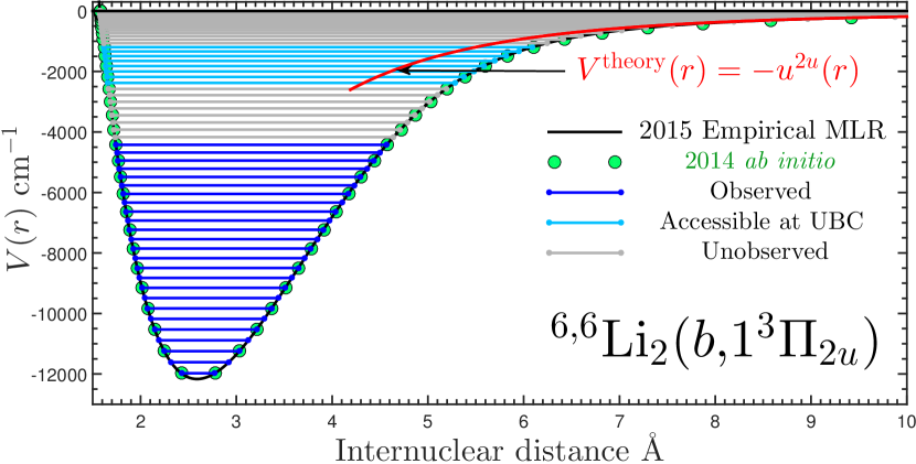
Figure 1: When considering the data for all isotopologues, levels up to $v=32$ have been observed. For ^6,6Li₂, levels $v=33-40$ are accessible by Kirk Madison’s group in University of British Columbia with the laboratory and method used in studies of the $A\left(1^{1}\Sigma_{u}^{+}\right)$ Gunton et al. (2013a) and $c\left(1^{3}\Sigma_{g}^{+}\right)$ Semczuk et al. (2013) states. The remainder of the levels have not been observed.

II Empirical potential and Born-Oppenheimer breakdown (BOB) corrections

We now wish to determine empirical functions for $V_{{\rm BO}}(r),\,\tilde{S}(r),$ and $\tilde{R}(r)$ that accurately reproduce all measured energies when using the Hamiltonian of Eq. 1.

There is a gap of more than 2000 cm^-1 ($>60$ THz) in experimental information between the highest observed level of Li${}_{2}\left(b,1^{3}\Pi_{u}\right)$, and its dissociation energy. This means that when building an empirical potential that aims to be relevant in the large data gap, it is very important to take great care in ensuring the potential behaves physically correctly in the extrapolation region. In 2011 the MLR (Morse/long-range) model was used in a fit to build empirical potentials from spectroscopic data for the $c\left(1^{3}\Sigma_{g}^{+}\right)-$states of ^6,6Li₂ and ^7,7Li₂, where there was a gap of more than $5000\>$cm^-1 between data near the bottom of the potential, and data at the very top Dattani and Le Roy (2011a). In 2013 spectroscopic measurements were made in the very middle of this gap Semczuk et al. (2013), and it was found that the vibrational energies predicted by the MLR potential from Dattani and Le Roy (2011a) were correct to within about 1 cm^-1. The present case for the $b$-state is in some sense more interesting because there is no data at the top helping to anchor the potential with the right shape near dissociation.

However, as for the $c$-state, the MLR model is still expected to be able to represent the physics in the extrapolation region faithfully since the correct theoretical long-range is built into the model. Having this long-range physics accurately built into the model is almost as helpful as having data in the long-range region, as was the case of the $c$-state. MLR-type empirical potentials have now successfully described spectroscopic data for many diatomic Le Roy et al. (2006); Roy and Henderson (2007); Salami et al. (2007); Shayesteh et al. (2007); Le Roy et al. (2009); Coxon and Hajigeorgiou (2010); Stein et al. (2010); Piticco et al. (2010); Le Roy et al. (2011); Ivanova et al. (2011); Dattani and Le Roy (2011a); Xie et al. (2011); Yukiya et al. (2013); Knöckel et al. (2013); Semczuk et al. (2013); Wang et al. (2013); Li et al. (2013a); Gunton et al. (2013a); Meshkov et al. (2014); Dattani (2014); Coxon and Hajigeorgiou (2015); Walji et al. (2015); Dattani (2015); Dattani et al. (2014) and polyatomic Li and Le Roy (2008); Li et al. (2010); Tritzant-Martinez et al. (2013); Wang et al. (2013); Li et al. (2013b); Ma et al. (2014) systems. Therefore, we will proceed to use the MLR model to describe $V{\rm{}_{{\rm BO}}}(r)$.

The MLR model is defined by

$$V_{{\rm MLR}}(r)\equiv\mathfrak{D}_{e}\left(1-\frac{u(r)}{u(r_{e})}e^{-\beta(r)y_{p}^{r_{e}}(r)}\right)^{2},$$ (19)

where $\mathfrak{D}_{e}$ is the dissociation energy, $r_{e}$ is the equilibrium internuclear distance, and the polynomial $\beta(r)$ is

$$\beta(r)\equiv\beta_{p,q}^{r_{{\rm ref}}}(r)\equiv\beta_{\infty}y_{p}^{r_{{\rm ref}}}(r)+\left(1-y_{p}^{r_{{\rm ref}}}(r)\right)\sum_{i=0}^{N_{\beta}}\beta_{i}\left(y_{q}^{r_{{\rm ref}}}(r)\right)^{i},$$ (20)

with

$$\beta_{\infty}\equiv\lim_{r\rightarrow\infty}\beta(r)=\ln\left(\frac{2\mathfrak{D}_{e}}{u(r_{e})}\right).$$ (21)

Equations 19 and 20 also depend on the radial variable

$$y_{n}^{r_{{\rm ref}}}(r)=\frac{r^{n}-r_{{\rm ref}}^{n}}{r^{n}+r_{{\rm ref}}^{n}},$$ (22)

where the reference distance $r_{{\rm ref}}$ is simply the equilibrium distance $r_{e}$ in most cases, but can be adjusted to optimize the fit to equation 19.

It is well known Le Roy et al. (2009); Dattani and Le Roy (2011a) that for large $r$ we have

$$V(r)\simeq\mathfrak{D}_{e}-u(r)+\cdots,$$ (23)

therefore the long-range behavior of the potential is defined by $u(r)$, and the short to mid-range behavior is defined by $\beta(r).$ In the $b\left(1^{3}\Pi_{u}\right)$ state, a spin-orbit interaction emerges at large internuclear distances, which splits the potential into four components. Therefore, four different potentials $V^{\Omega_{u}}(r)$ can be defined to have the same $\beta(r)$ defining the short-range behavior where there is no significant splitting, and to have four different $u^{{}^{3}\Pi_{u},\Omega_{u}}(r)$ defining the long-range where the splitting occurs.

For large $r$ where the spin-orbit interaction becomes strong, it is dangerous to label the spin angular momentum $S$ and orbital angular momentum $\Lambda$ separately, as in the molecular term symbol ${}^{2S+1}\Lambda$. Instead, these two momenta are combined into a total electronic angular momentum $\Omega$. For ${}^{3}\Pi_{u}$, $S=1$ and $\Lambda=1$, so there are states with four possible symmetries in the $\Omega$ representation: $0_{u}^{+}$, $0_{u}^{-}$, $1_{u}$, and $2_{u}$. Each of these four states has a slightly different behavior at large internuclear distances, due to coupling with states that have the same symmetry in the $\Omega$ representation, but different symmetry in the $\Lambda$ representation. This coupling has been described in Aubert-Frécon et al. (1998) and has been used for building appropriate analytic empirical potentials for the $A\left(1^{1}\Sigma_{u}^{+}\right)$ Le Roy et al. (2009); Gunton et al. (2013a) and $c\left(1^{1}\Sigma_{u}^{+}\right)$ Dattani and Le Roy (2011a); Semczuk et al. (2013) states of Li₂. The long-range function $u(r)$ is defined separately for each spin-orbit state:

$$u(r) = \begin{cases}u^{b,0_{u}^{+}}(r)&,\,0_{u}^{+}\\ u^{b,0_{u}^{-}}(r)&,\,0_{u}^{-}\\ u^{b,1_{u}}(r)&,\,1_{u}\\ u^{b,2_{u}}(r)&,\,2_{u}.\end{cases}$$ (24)

Each of these functions is an eigenvalue of a matrix $\mathbf{u}^{\Omega_{u}}$ for each $\Omega_{u}$ state. These matrices are given in the subsections below, in terms of the (positive) spin-orbit splitting energy $\Delta E$, and neglecting exchange interaction terms.

II.1 The $0_{u}^{+}$ states

In addition to the $b($1${}^{3}\Pi_{u})$ state, the other $\Lambda$ state that can give rise to $0_{u}^{+}$ symmetry is the $A(1^{1}\Sigma_{u}^{+})$ state Jones et al. (2006). The interstate coupling is therefore given by the $2\times 2$ matrix Aubert-Frécon et al. (1998):

$$\mathbf{u}^{0_{u}^{+}}(r) = \begin{pmatrix}\frac{1}{3}{\displaystyle\sum_{\begin{subarray}{c}m=3,6,8\\ 9,10,11,\ldots\end{subarray}}}\frac{C_{m}^{A\left(1{}^{1}\Sigma_{u}^{+}\right)}+2C_{m}^{b\left(1{}^{3}\Pi_{u}\right)}}{r^{m}}&\quad\;\frac{\sqrt{2}}{3}{\displaystyle\sum_{\begin{subarray}{c}m=3,6,8\\ 9,10,11,\ldots\end{subarray}}}\frac{C_{m}^{A\left(1{}^{1}\Sigma_{u}^{+}\right)}-C_{m}^{b\left(1{}^{3}\Pi_{u}\right)}}{r^{3}}\\ \frac{\sqrt{2}}{3}{\displaystyle\sum_{\begin{subarray}{c}m=3,6,8\\ 9,10,11,\ldots\end{subarray}}}\frac{C_{m}^{A\left(1{}^{1}\Sigma_{u}^{+}\right)}-C_{m}^{b\left(1{}^{3}\Pi_{u}\right)}}{r^{m}}&\qquad\quad\Delta E+\frac{2}{3}{\displaystyle\sum_{\begin{subarray}{c}m=3,6,8\\ 9,10,11,\ldots\end{subarray}}}\frac{C_{m}^{A\left(1{}^{1}\Sigma_{u}^{+}\right)}+C_{m}^{b\left(1{}^{3}\Pi_{u}\right)}}{r^{m}}\end{pmatrix},$$ (25)

where the lower energy eigenvalue $u^{A,0_{u}^{+}}(r)$ comes from $A\left(1^{1}\Sigma_{u}^{+}\right)$ and approaches the dissociation limit of Li$\left(2^{2}S_{\nicefrac{{1}}{{2}}}\right)+\mbox{Li}\left(2^{2}P{}_{\nicefrac{{1}}{{2}}}\right)$, and the higher energy eigenvalue $u^{b,0_{u}^{+}}(r)$ comes from $b\left(1^{3}\Pi_{u}\right)$ and approaches the dissociation limit of Li$\left(2^{2}S_{\nicefrac{{1}}{{2}}}\right)+\mbox{Li}\left(2^{2}P{}_{\nicefrac{{3}}{{2}}}\right)$ Jones et al. (2006).

II.2 The $0_{u}^{-}$ states

In addition to the $b($1${}^{3}\Pi_{u})$ state, the other $\Lambda$ state that can give rise to $0_{u}^{-}$ symmetry is the $2a(2^{3}\Sigma_{u}^{+})$ state Jones et al. (2006). The interstate coupling is therefore given by the $2\times 2$ matrix Aubert-Frécon et al. (1998):

$$\mathbf{u}^{0_{u}^{-}}(r) = \begin{pmatrix}\frac{1}{3}{\displaystyle\sum_{\begin{subarray}{c}m=3,6,8\\ 9,10,11,\ldots\end{subarray}}}\frac{C_{m}^{2a\left(2{}^{3}\Sigma_{u}^{+}\right)}+2C_{m}^{b\left(1{}^{3}\Pi_{u}\right)}}{r^{m}}&\quad\;\frac{\sqrt{2}}{3}{\displaystyle\sum_{\begin{subarray}{c}m=3,6,8\\ 9,10,11,\ldots\end{subarray}}}\frac{C_{m}^{2a\left(2{}^{3}\Sigma_{u}^{+}\right)}-C_{m}^{b\left(1{}^{3}\Pi_{u}\right)}}{r^{3}}\\ \frac{\sqrt{2}}{3}{\displaystyle\sum_{\begin{subarray}{c}m=3,6,8\\ 9,10,11,\ldots\end{subarray}}}\frac{C_{m}^{2a\left(2{}^{3}\Sigma_{u}^{+}\right)}-C_{m}^{b\left(1{}^{3}\Pi_{u}\right)}}{r^{m}}&\qquad\quad-\Delta E+\frac{2}{3}{\displaystyle\sum_{\begin{subarray}{c}m=3,6,8\\ 9,10,11,\ldots\end{subarray}}}\frac{C_{m}^{2a\left(2{}^{3}\Sigma_{u}^{+}\right)}+C_{m}^{b\left(1{}^{3}\Pi_{u}\right)}}{r^{m}}\end{pmatrix},$$ (26)

where the lower energy eigenvalue comes from $b\left(1^{3}\Pi_{u}\right)$ and approaches the dissociation limit of Li$\left(2^{2}S_{\nicefrac{{1}}{{2}}}\right)+\mbox{Li}\left(2^{2}P{}_{\nicefrac{{1}}{{2}}}\right)$, and the higher energy eigenvalue comes from $2a\left(2^{3}\Sigma_{u}^{+}\right)$ and approaches the dissociation limit of Li$\left(2^{2}S_{\nicefrac{{1}}{{2}}}\right)+\mbox{Li}\left(2^{2}P{}_{\nicefrac{{3}}{{2}}}\right)$ Jones et al. (2006).

II.3 The $1_{u}$ states

In addition to the $b($1${}^{3}\Pi_{u})$ state, the other $\Lambda$ states that can give rise to $1_{u}$ symmetry are the $2a\left(2^{3}\Sigma_{u}^{+}\right)$ state and the $B\left(1{}^{1}\Pi_{u}\right)$state Jones et al. (2006). The interstate coupling is therefore given by the $3\times 3$ matrix Aubert-Frécon et al. (1998):

$$\mathbf{u}^{1_{u}}(r)=$$ (27)

$$\negthickspace\negthickspace\left(\begin{array}[]{ccc}\frac{1}{3}{\displaystyle\sum_{m}\frac{C_{m}^{2a\left(2{}^{3}\Sigma_{u}^{+}\right)}+C_{m}^{B\left(1{}^{1}\Pi_{u}\right)}+C_{m}^{b\left(1{}^{3}\Pi_{u}\right)}}{r^{m}}}&\frac{1}{3\sqrt{2}}{\displaystyle\sum_{m}\frac{-2C_{m}^{2a\left(2{}^{3}\Sigma_{u}^{+}\right)}+C_{m}^{B\left(1{}^{1}\Pi_{u}\right)}+C_{m}^{b\left(1,^{3}\Pi_{u}\right)}}{r^{m}}}&\frac{1}{\sqrt{6}}{\displaystyle\sum_{m}\frac{-C_{m}^{B\left(1,^{1}\Pi_{u}\right)}+C_{m}^{b\left(1,^{3}\Pi_{u}\right)}}{r^{m}}}\\ \frac{1}{3\sqrt{2}}{\displaystyle\sum_{m}\frac{-2C_{m}^{2a\left(2{}^{3}\Sigma_{u}^{+}\right)}+C_{m}^{B\left(1{}^{1}\Pi_{u}\right)}+C_{m}^{b\left(1{}^{3}\Pi_{u}\right)}}{r^{m}}}&\Delta E_{{\rm SO}}+\frac{1}{6}{\displaystyle\sum_{m}\frac{4C_{m}^{2a\left(2{}^{3}\Sigma_{u}^{+}\right)}+C_{m}^{B\left(1{}^{1}\Pi_{u}\right)}+C_{m}^{b\left(1{}^{3}\Pi_{u}\right)}}{r^{m}}}&\frac{1}{2\sqrt{3}}{\displaystyle\sum_{m}\frac{-C_{m}^{B\left(1{}^{1}\Pi_{u}\right)}+C_{m}^{b\left(1{}^{3}\Pi_{u}\right)}}{r^{m}}}\\ \frac{1}{\sqrt{6}}{\displaystyle\sum_{m}\frac{-C_{m}^{B\left(1{}^{1}\Pi_{u}\right)}+C_{m}^{b\left(1{}^{3}\Pi_{u}\right)}}{r^{m}}}&\frac{1}{2\sqrt{3}}{\displaystyle\sum_{m}\frac{-C_{m}^{B\left(1{}^{1}\Pi_{u}\right)}+C_{m}^{b\left(1{}^{3}\Pi_{u}\right)}}{r^{m}}}&-\Delta E+\frac{1}{2}{\displaystyle\sum_{m}\frac{C_{m}^{B\left(1{}^{1}\Pi_{u}\right)}+C_{m}^{b\left(1{}^{3}\Pi_{u}\right)}}{r^{m}}}\end{array}\right),$$ (28)

where the lowest energy eigenvalue comes from $b\left(1^{3}\Pi_{u}\right)$ and approaches the dissociation limit of Li$\left(2^{2}S_{\nicefrac{{1}}{{2}}}\right)+\mbox{Li}\left(2^{2}P{}_{\nicefrac{{1}}{{2}}}\right)$, and the middle and highest energy eigenvalues come from $B\left(1^{1}\Pi_{u}\right)$ and $2a\left(2^{3}\Sigma_{u}^{+}\right)$ respectively and both approach the dissociation limit of Li$\left(2^{2}S_{\nicefrac{{1}}{{2}}}\right)+\mbox{Li}\left(2^{2}P{}_{\nicefrac{{3}}{{2}}}\right)$ Jones et al. (2006).

II.4 The $2_{u}$ state

The $2_{u}$ state approaching the dissociation limit of $2S+2P$ is alone in its symmetry, and approaches Li$\left(2^{2}S_{\nicefrac{{1}}{{2}}}\right)+\mbox{Li}\left(2^{2}P{}_{\nicefrac{{3}}{{2}}}\right)$ Jones et al. (2006). It has the long-range function Tang et al. (2011):

$$u^{2_{u}}(r) = -\left(\Delta E-\sum_{\begin{subarray}{c}m=3,6,8,\\ 9,10,11,\ldots\end{subarray}}\frac{C_{m}^{b\left(1{}^{3}\Pi_{u}\right)}}{r^{m}}\right)$$ (29)

$$= -\left(\Delta E-\frac{C_{3}^{b\left(1{}^{3}\Pi_{u}\right)}}{r^{3}}-\frac{C_{6}^{b\left(1{}^{3}\Pi_{u}\right)}}{r^{6}}-\frac{C_{8}^{b\left(1{}^{3}\Pi_{u}\right)}}{r^{8}}-\frac{C_{9}^{b\left(1{}^{3}\Pi_{u}\right)}}{r^{9}}-\frac{C_{10}^{b\left(1{}^{3}\Pi_{u}\right)}}{r^{10}}-\frac{C_{11}^{b\left(1{}^{3}\Pi_{u}\right)}}{r^{11}}\cdots.\right)$$ (30)

II.5 All four $\Omega_{u}$ states combined

One can imagine an experiment which obtains spectroscopic measurements for all of the four $\Omega_{u}$ states, and fits to all of this data simultaneously by using the appropriate eigenvalues of the $8\times 8$ matrix below:

$$u = \left(\begin{array}[]{cccc}\mathbf{u^{0_{u}^{+}}}\\ &\mathbf{u^{0_{u}^{-}}}\\ &&\mathbf{u^{1_{u}}}\\ &&&u^{2_{u}}\end{array}\right)$$ (35)

$$= \left(\begin{array}[]{cccccccc}u_{11}^{0_{u}^{+}}&u_{12}^{0_{u}^{+}}\\ u_{21}^{0_{u}^{+}}&u_{22}^{0_{u}^{+}}\\ &&u_{11}^{0_{u}^{-}}&u_{12}^{0_{u}^{-}}\\ &&u_{21}^{0_{u}^{-}}&u_{22}^{0_{u}^{-}}\\ &&&&u_{11}^{1_{u}}&u_{12}^{1_{u}}&u_{13}^{1_{u}}\\ &&&&u_{21}^{1_{u}}&u_{22}^{1_{u}}&u_{23}^{1_{u}}\\ &&&&u_{31}^{1_{u}}&u_{32}^{1_{u}}&u_{33}^{1_{u}}\\ &&&&&&&u^{2_{u}}\end{array}\right).$$ (44)

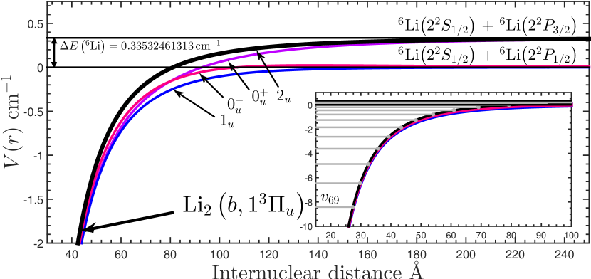
Figure 2: In the long-range region, the splitting of the $b\left(1^{3}\Pi_{u}\right)$ state into four spin-orbit components becomes increasingly obvious. This is well beyond the region where data is available, so our empirical potential fits to a model with the simplest long-range potential energy function (the $2_{u}$ state, since there are no other $2_{u}$ states that are nearby in energy, see Eqs. 29-44). The fine-structure splitting of $0.33532461313$ cm^-1 comes from measurements in Brown et al. (2013).

However, Fig. 1 shows the data region, and Fig. 2 shows that the spin-orbit splitting does not seem to become apparent until well past this region. Since the measurements that have been done on the $b$-state thus far are far away from the effect of the spin-orbit splitting, we choose to use the simplest spin-orbit long-range function: $u^{b,2_{u}}(r)$.

II.6 Quadratic corrections and damping functions

Since the leading term not shown in Eq. 23 is $\frac{u(r)^{2}}{4\mathfrak{D}_{e}}$, the contribution of the $C_{3}$ terms to the long-range form of the potential, will interfere with the desired $C_{6}$ and $C_{8}$ terms, and all $C_{9}$ and $C_{11}$ terms will therefore have spurious contributions from the cross-terms formed by the products of the $C_{3}$ terms with the $C_{6}$ and $C_{8}$ terms respectively. We fix this in the same way as was done for $C_{6}$ and $C_{9}$ in Dattani et al. (2008); Le Roy et al. (2009); Dattani and Le Roy (2011a); Semczuk et al. (2013); Gunton et al. (2013a), by applying a transformation to all $C_{6}$, $C_{9}$, and this time also $C_{11}$ terms:

$$C_{6} \rightarrow C_{6}+\frac{C_{3}^{2}}{4\mathfrak{D}_{e}}$$ (45)

$$C_{9} \rightarrow C_{9}+\frac{C_{3}C_{6}}{2\mathfrak{D}_{e}},$$ (46)

$$C_{11} \rightarrow C_{11}+\frac{C_{3}C_{8}}{2\mathfrak{D}_{e}}.$$ (47)

where the transformation in Eq. 45 has to be made first due to Eq. 46’s dependence on $C_{6}$.

Additionally, The long-range formulas in terms of $C_{m}$ constants in the above sub-sections were derived under the assumption that two free atoms are interacting with each other, and there is no overlap of the electrons’ wavefunctions as in a bound molecule. To take into account the effect of electron overlap, we use the damping function form from Le Roy et al. (2011):

$$C_{m} \rightarrow C_{m}D_{m}^{(s)}\left(r\right)$$ (48)

$$D_{m}^{(s)}\left(r\right) \equiv \left(1-e^{-\left(\frac{b^{(s)}\rho r}{m}+\frac{c^{(s)}\left(\rho r\right)^{2}}{\sqrt{m}}\right)}\right)^{m+s},$$ (49)

where for interacting atoms A and B, $\rho\equiv\rho_{{\rm AB}}=\frac{2\rho_{{\rm A}}\rho_{{\rm B}}}{\rho_{{\rm A}}\rho_{{\rm B}}},$ in which $\rho_{{\rm X}}\equiv\left(\nicefrac{{I^{{\rm X}}}}{{I^{{\rm H}}}}\right)^{\nicefrac{{2}}{{3}}}$ is defined in terms of the ionization potentials of atom X, denoted $\left(I^{{\rm X}}\right)$, and hydrogen$\left(I^{{\rm H}}\right)$. We use $s=-1$, which as shown in Le Roy et al. (2011), means that the MLR potential in Eq. 19 has the physically desired behavior $V\propto\nicefrac{{1}}{{r^{2}}}$ in the limit as $r\rightarrow 0$. For $s=-1$, the system independent parameters take the values $b^{(-1)}=3.30$, and $c^{(-1)}=0.423$ Le Roy et al. (2011).

II.7 Long-range constants

In previous studies of the $A(1^{1}\Sigma_{u}^{+})$ state Le Roy et al. (2009); Gunton et al. (2013b) and $c(1^{3}\Sigma_{g}^{+})$ state Dattani and Le Roy (2011a); Semczuk et al. (2013), it was found that the most precise theoretical values of $C_{3}$ known at those times Tang et al. (2010b, 2009a) did not fit as well with the measurements of the high-lying vibrational levels near the dissociation, as the values of $C_{3}$ obtained by setting it as a free parameter determined by a least-squares fit to the data.

However, for the $b\left(1^{3}\Pi_{u}\right)$-state, no measurements of such high-lying vibrational levels have been made, so such an “empirical fit” to $C_{3}$ is impossible, and we will have to use the most precise theoretical value known. For ^7,7Li₂ this is the value from Tang et al. (2010b) and for ^6,6Li₂ this is an unpublished value from Tang calculated in 2015 Tang (2015). These values are listed in Table 2, along with the theoretical values for the higher-order $C_{m}$ constants used in our analysis (it has not yet been possible to fit these higher-order $m>3$ constants to spectroscopic data in any direct-potential-fit analysis, so they are held fixed). For $m>8$, no finite-mass corrections have been calculated yet.

Table 2: The best currently available long-range constants and their sources (in Hartree atomic units). ^∞Li₂ represents a Li₂ molecule where both nuclei have infinite mass, since finite mass corrections have not yet been calculated for $C_{m}$ coefficients with $m\geq 9$.

	$A\left(1^{1}\Sigma_{u}\right)$		$2a\left(2^{3}\Sigma_{u}\right)$		$B\left(1^{1}\Pi_{u}\right)$		$b\left(1^{3}\Pi_{u}\right)$
	6,6Li2	7,7Li2	6,6Li2	7,7Li2	6,6Li2	7,7Li2	6,6Li2	7,7Li2	Ref.
$C_{3}$	$11.0009$ Tang (2015)	$11.0007$ Tang (2015)	$-11.0009$ Tang (2015)	$-11.0007$ Tang et al. (2010b)	$-5.5005$ Tang (2015)	$-5.5004$ Tang (2015)	5.5005 Tang (2015)	5.5004 Tang (2015)	-
$C_{6}$	2076.19(7)	2076.08(7)	2076.19(7)	2076.08(7)	1407.20(2)	1407.15(5)	1407.20(2)	1407.15(5)	Tang et al. (2009b)
$C_{8}$	274137(6)	274128(5)	991104(5)	991075(6)	48566.9(4)	48566.4(2)	103053(1)	103052(1)	Tang et al. (2009b)
	∞Li2		∞Li2		∞Li2		∞Li2
$C_{9}$	2.2880(2)$\times 10^{5}$		$-2.2880(2)$$\times 10^{5}$		$-5.173(1)$$\times 10^{4}$		5.173(1)$\times 10^{4}$		Tang et al. (2011)
$C_{10}$	3.0096$\times 10^{7}$		$-1.2113$$\times 10^{8}$		8.9295$\times 10^{6}$		9.1839$\times 10^{5}$		Zhang et al. (2007)
$C_{11}$	$-5.930\times 10^{7}$		$-5.0321$$\times 10^{8}$		$-9.924\times 10^{7}$		2.652$\times 10^{7}$		Tang et al. (2011)

 

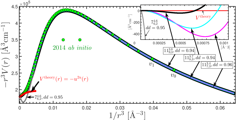
Figure 3: Various $(N_{\beta})_{p,q}^{r_{{\rm ref}}}$ models with the same quality of fit are in agreement with each other, until large values of $r$ at which the $N_{\beta}=7$ model dips significantly below the red curve representing the theoretical long-range behavior. This dip was obvious in the $-r^{3}V(r)$ vs $\nicefrac{{1}}{{r^{3}}}$ plots for all models mentioned in the text except for the three $N_{\beta}=11$ cases shown. The inset shows $-r^{3}V(r)$ for the four mentioned models, subtracted from the red theoretical curve. All models match the theory for very large $r$ (small $\nicefrac{{1}}{{r^{3}}}$), but the cases with higher $p$ and/or $q$ match the theory for a much larger range of $r$. Each green circle represents an outer classical turning point of the ab initio potential. In the inset, the ab initio values lie too high above 0 to be seen.

II.8 Dissociation energy $\mathfrak{D}_{e}$

At the time of carrying out our analysis, the best experimental value for $\mathfrak{D}_{e}$ of which we were aware, was the 1983 value from Engelke and Hage (1983): 12145$\pm$200 cm^-1. In a recent study on BeH Dattani (2015), the gap between the highest observed level and the dissociation asymptote was $\sim 1000$ cm^-1, and the fitted value of $\mathfrak{D}_{e}$ varied by about $400$ cm^-1 as parameters such as $r_{{\rm ref}}$, $p$, and $q$ were changed. For the present case of the $b$-state of Li₂, the data region stops more than 4000 cm^-1 below the dissociation asymptote, so we do not expect to be able to determine $\mathfrak{\mathfrak{D}_{e}}$any more precisely than the 1983 experimental value. However, we still tried, by letting $\mathfrak{D}_{e}$ be a free parameter, and we indeed found that the fitted values varied by more than $400$ cm^-1. Therefore, it might make sense to use experimental value from Engelke and Hage (1983) which was claimed to be within 400 cm^-1.

However, it is expected that the ab initio value from Musial and Kucharski (2014) correct to within much less than 400 cm^-1. This is because we systematically checked the ab initio $\mathfrak{D}_{e}$ values for all electronic Li₂ states calculated in Musial and Kucharski (2014), and found that they were at most 68 cm^-1 different from the best experimental value, even when the experimental values were known to as high of a precision as 0.0023 cm^-1 (see Table 3). Furthermore, the ab initio value for the $b$-state was within the 400 cm^-1 confidence interval given by the 1983 experimental value Engelke and Hage (1983) discussed in the previous paragraph. Therefore, we decided to fix our $\mathfrak{\mathfrak{D}_{e}}$ value at the ab initio value of 12166 cm^-1 and to only allow the other parameters be free parameters for the remainder of the fitting analysis.

After the completion of this work, we discovered that a much less known paper co-authored by one of the same authors from Engelke and Hage (1983), reported a more precise $\mathfrak{D}_{e}$ value of (12180.6$\pm 0.6$) cm^-1 just over 4 years afterwards Schmidt et al. (1988), but it is not clear in the paper how this value, nor its uncertainty is obtained. Particularly, it is not clear whether this is a purely empirical value, or if it also uses the ab inito potential which is part of the subject of the paper.

Table 3: Dissociation energies $\mathfrak{D}_{e}$ in cm^-1 of various electronic states of Li₂. “obs - calc” denotes the ab initio value subtracted from the empirical value. Numbers in parenthesis indicate the experimental uncertainty in the last digit(s) shown. Where possible, ^6,6Li₂ values were used. for the empirical values. When empirical values for the $\mathfrak{D}_{e}$ of ^6,6Li₂ were not available, the empirical value for ^7,7Li₂ is given. All ab initio values are for ^∞Li₂ which is a hypothetical Li₂ molecule with infinite mass.

$2S+2S$	$X(1^{1}\Sigma_{g}^{+})$		$a(1^{3}\Sigma_{u}^{+})$
ab initio Musial and Kucharski (2014)	8466.		334.
empirical	8516.	7800(23) Gunton et al. (2013a)	333.	7795(62) Semczuk et al. (2013)
obs - calc	51.		0.
$2S+2P$	$A(1^{1}\Sigma_{u}^{+})$		$B(1^{1}\Pi_{u})$		$2X(2^{1}\Sigma_{g}^{+})$		$C(1^{1}\Pi_{g})$		$b(1^{3}\Pi_{u})$		$c(1^{3}\Sigma_{g}^{+})$
ab initio Musial and Kucharski (2014)	9356.		2930.		3289.		1426.		12166.		7080.
empirical	9353.	1795(28) Gunton et al. (2013a)	2984.	444(110) Huang and Le Roy (2003)	3318(66) He et al. (1991); Barakat et al. (1986)		1422.	5(3) Miller et al. (1990)	12145.	(200) Engelke and Hage (1983)	7092.	4926(86) Semczuk et al. (2013)
obs - calc	-3.		54.		30.		-3.		-21.		12.
$2S+3S$	$3X(3^{1}\Sigma_{g}^{+})$ (1st min.)				$2A(1^{1}\Sigma_{u}^{+})$ (1st min.)				$2A(1^{1}\Sigma_{u}^{+})$ (2nd min.)
ab initio Musial and Kucharski (2014)	8290.				5608.				5389.
empirical	8317. Bernheim et al. (1982, 1983)				5615. S et al. (2000); Kubkowska et al. (2007)				5321. S et al. (2000); Kubkowska et al. (2007)
obs - calc	27.				7.				-68.
$2S+3P$	$4X(4^{1}\Sigma_{g}^{+})$ (1st min.)				$2B(2^{1}\Pi_{u})$		$2C(2^{1}\Pi_{g})$		$D(1{}^{1}\Delta_{g})$		$2d(2{}^{3}\Pi_{g})$
ab initio Musial and Kucharski (2014)	8380.				6481.		7773.		9592.		8505.
empirical	8349. Bernheim (1981a)				6455.	Bernheim (1981b)	7773.	7(3) Kubkowska et al. (2007)	9579.	Linton et al. (1993)	8484.	Bernheim (1981b)
obs - calc	-31.				-26.		1.		-13.		-21.

 

II.9 Choice of model parameters

Using the Hamiltonian of Eq. 1, we fit the parameters of Eq. 19 to the 1234 data, with the involved energy levels of the upper states $2^{3}\Pi_{g}$ and $1^{3}\Delta_{g}$ treated as free parameters. All fits to the data were done using the freely available program ${\tt DPotFit}\,2.0$ Le Roy et al. (2013). Starting parameters for the fits to Eq. 19 were found by fitting to an RKR potential using the freely available program ${\tt betaFit\,2.1}$ LeRoy (2012). The RKR potential was made using the program ${\tt RKR1\,2.0}$ LeRoy (2004) using the Dunham coefficients found in Table IV of Linton et al. (1992).

The quality of a fit was determined by the dimensionless root-mean-square-deviation ($\overline{dd}$) which scales each deviation between an energy predicted by the model ($E_{{\rm calc}}$) and the corresponding measurement ($E_{{\rm obs}})$, by the uncertainty of the measurement ($u_{{\rm obs}}$), for all $N_{{\rm data}}$ measurements:

$$\overline{dd}\equiv\sqrt{\frac{1}{N_{{\rm data}}}\sum_{i=1}^{N_{{\rm data}}}\left(\frac{E_{{\rm calc}}(i)-E_{{\rm obs}}(i)}{u_{{\rm obs}}(i)}\right)^{2}}.$$ (50)

In previous studies of the $A(1^{1}\Sigma_{u}^{+})$ state Gunton et al. (2013b) and $c(1^{3}\Sigma_{g}^{+})$ state Semczuk et al. (2013), it was determined that there was no benefit in including long-range terms beyond $C_{8}$, because the data for the high-lying rovibrational energies began to deviate from the theoretical long-range potential energy curve at distances shorter than the distance where $C_{9}$ began to give a noticeable effect on the long-range function $u_{{\rm LR}}(r)$ (see Fig. 6 of Semczuk et al. (2013) for example) .

However, for the $b$-state, no data exists in the long-range region, so it might make more sense to include more $C_{m}$ terms in $u_{{\rm LR}}(r)$ in order to anchor the potential somewhat appropriately in the $>$2500 cm^-1 gap at the top of the potential well where no data exists to guide the potential. Nevertheless, we first followed the $A-$ and $c-$state studies and only used up to $C_{8}$. We found an excellent fit with $\overline{dd}=0.95$ with only $N_{\beta}=7$, $p=6,$ $q=2$. However, the long-range behavior of this potential was in vast disagreement with the long-range behavior expected by theory (see Fig. 3). This is because with $(p,q)=(6,2)$, the long-range form of the potential described in Eq. 23 does not “turn on” until too high a value of $r$ (a larger value of $r$ is needed for $y_{p}^{r_{{}_{{\rm ref}}}}(r)$ and $y_{q}^{r_{{}_{{\rm ref}}}}(r)$ to become sufficiently close to their limiting values of 1.

We can often encourage the the long-range form to “turn on” earlier by increasing $p$ and/or $q$, which often comes with the expense of requiring a higher polynomial degree $N_{\beta}$ to recover the same $\overline{dd}$. We explored models with $p\in\{6,7,8,9\}$ and $q\in\{2,3\}$, including the $C_{9}$ term in $u_{{\rm LR}}$ for $p\geq 7$, $C_{10}$ for $p\geq 8$, and $C_{11}$ for $p=9$. Ideally we would always use as many $C_{m}$ constants as are known, but as explained in Le Roy et al. (2009); Dattani and Le Roy (2011a), the value of $p$ in Eqs. 19 and 20 need to satisfy $p>m_{{\rm last}}-m_{{\rm first}}$ where $m_{{\rm last}}$ and $m_{{\rm first}}$ represent respectively the last and first $C_{m}$ terms included in $u_{{\rm LR}}(r)$. We also note that $C_{12}$ for the Li$\left(2^{2}S\right)+\mbox{Li}\left(2^{2}P\right)$ asymptote is not available, as far as we know.

We found that if $p<9$ and/or $q<3$, the long-range behavior does not turn on until about $r=32$ Å (in the very best cases), while the $m$-dependent Le Roy radius Tsai et al. (1994) calculated from the radial expectation values found in Zhang et al. (2007) suggests that the long-range behavior should turn on before $r=10$ Å. With $(p,q)=(9,3)$, we found a fit with $N_{\beta}=11$ and $\overline{dd}=0.94$, where the long-range behavior turns on at about $r=20$ Å (see Fig 3). Increasing $q$ to 4 would likely turn the long-range behavior on at closer to the $m$-dependent Le Roy radius, but no $(p,q)=(9,4)$ fits with $N_{\beta}\leq 11$ had a $\overline{dd}<1$ and we needed to push to $N_{\beta}\geq 13$ in order to match the $\overline{dd}$ of the best $(p,q,N_{\beta})=(9,3,11)$ fits. Using such a high-degree polynomial, when the data only required $N_{\beta}=7$ for a good fit, can be dangerous in terms of the potential’s extrapolation in the regions neither constrained by data nor built-in $C_{m}$ constants. In this respect, we also tried $(p,q)=(9,3)$ fits with $N_{\beta}=10$ for various $r_{{\rm ref}}$ values, but no such fit had a $\overline{dd}<1$.

II.10 Born-Oppenheimer breakdown (BOB) corrections

With our best MLR model: MLR${}_{p,q}^{r_{{\rm ref}}}\left(N_{\beta}\right)=\mbox{MLR${}_{9,3}^{3.8}\left(11\right)$}$, we attempted to add adiabatic ($\tilde{S}(r)$, from Eq. 17) and non-adiabatic ($\tilde{R}(r)$, from Eq. 18) BOB corrections with the same model functions as used in previous studies of Li₂ since these models were improved in 2009 Le Roy et al. (2009); Dattani and Le Roy (2011b); Semczuk et al. (2013); Gunton et al. (2013a). It was surprising that despite there being 599 ⁶Li₂ data $\left(\mbox{with }v_{{\rm max}}=9,\,N_{{\rm max}}=46\right)$ and 696 ⁷Li₂ data $\left(\mbox{with }v_{{\rm max}}=27,\,N_{{\rm max}}=27\right)$, adding BOB correction functions did not improve the fit. Even when fitting to 3 adiabatic BOB parameters and 3 non-adiabatic BOB parameters, the $\overline{dd}$ went down by less than 1%. This is unexpected when there is just as much data for each isotopologue, and there is such a big difference in the highest $v$ and $N$ levels observed for each isotopologue.

Nevertheless, it seems that the isotopologue shifts due to the kinetic energy term in the Hamiltonian, and due to the mass-dependent BOB corrections incorporated from Eqs. 10 and 14, are the only significant sources of energy difference between ⁶Li₂ and ⁷Li₂ for the $b$-state (within our data’s precision). This may also explain why the ab initio potentials Musial and Kucharski (2014) calculated assuming an infinite molecular mass managed to predict both the ⁶Li₂ and ⁷Li₂ energies so fabulously (see discussion in Section II.12 and Table IV), while the ab initio BOB correction functions for the not much lighter molecule BeH, were so crucial in matching the ro-vibrational energies predicted from the ab initio and empirical potentials Dattani (2015); Koput (2011). Therefore, the final potential that we recommend, which is the same for both ⁶Li₂ and ⁷Li₂ in the $b$-state except for the small mass-dependent contributions coming from the kinetic energy and the un-colored terms in Eq. 16, does not contain any empirically fitted $\tilde{S}(r)$ and $\tilde{R}(r)$ BOB correction functions.

II.11 Sequential rounding and re-fitting (SRR)

Observing the predicted values for $r_{e}$ yielded by 139 different fits which had $\overline{dd}<0.957$ (within 1.5% of the optimal fit, which had $\overline{dd}=0.942$), we see that no fit predicted an $r_{e}$ outside the range $(2.589\,825<r_{e}<2.589\,871)$ Å, regardless of the values of $(p,q,r_{{\rm ref}},N_{\beta})$, though the more extreme predictions of $r_{e}$ within this range corresponded to fits with $N_{\beta}\leq 9$. Based on this observation, we recommend the value $r_{e}=(2.589\,848\pm 0.000\,023)$ Å, which is the average of these upper and lower bounds, with the uncertainty being the distance from the average to either bound.

We then re-fitted the potential to the data, but with $r_{e}$ fixed at 2.589848 Å, once with the ${\tt DPotFit}$ setting ${\tt IROUND=-1}$ and once with ${\tt IROUND=+1}$ in order to implement the SRR procedure described in Le Roy (1998) and in the ${\tt DPotFit}$ manual Le Roy et al. (2013). Neither of these cases affected the 3-digit value $\overline{dd}=0.942$. The ${\tt IROUND=-1}$ fit ended up with 2 more total digits than when ${\tt IROUND=+1}$ was used, but had a lower $\overline{dd}$ in the 4th digit, and has the more elegant feature that the number of digits in $\beta_{i}$ decreases monotonically with increasing $i$. Therefore, we recommend the potential with ${\tt IROUND=-1}$, whose parameters are listed in Table 4.

II.12 Vibrational energy spacings of the recommended Li${}_{2}\left(b,^{3}\Pi_{u}\right)$ potential, and comparison to best ab initio potential

Very recently, a review paper on the 5e^- systems BeH, BeD, and BeT Dattani (2015) revealed that the state of the art ab initio potentials Koput (2011) (which used MR-ACPF/aug-cc-pCV7Z(i), a further estimate of electron correlation effects beyond the approximations of MR-ACPF, second-order DKH scalar relativistic corrections, and mass-dependent BOB corrections), predicted vibrational energy spacings with up to at most 1.8 cm^-1 discrepancy with the state of the art empirical potential in the region for which vibrational energies had been measured. The ab initio potential also predicted the existence of one more vibrational level than the empirical potential, in the cases of BeH and BeD. This was all for the ground electronic state $X\left(1{}^{2}\Sigma^{+}\right)$, so it is of interest to see how well the most state-of-the-art ab initio potential for the 6e^- Li₂ excited state $b\left(1{}^{3}\Pi_{u}\right)$ will be.

A Fock space MRCC method based on the (2,0) sector of the Fock space, called FS-CCSD(2,0) Musial (2012), was recently implemented and used to calculate potential energy curves for many excited states of Li₂ Musial and Kucharski (2014) with the ANO-RCC basis set Veryazov et al. (2004). While in principle possible, DKH and BOB corrections have not been made in any Li₂ ab initio calculations to date. However, fortunately we found in Section II.10 that the addition of $\tilde{S}(r)$ or $\tilde{R}(r)$ functions did not significantly improve the fit to the data, meaning that Born-Oppenheimer breakdown beyond the effects included from Eqs. 10 and 14 do not seem to have a big effect in this particular state of Li₂, at least in the data region. Said another way, the ab initio Born-Oppenheimer potential is expected to give good predictions of the energies of ^6,6Li₂ and ^7,7Li₂, with mass-dependent differences accounted for only by the Hamiltonian’s kinetic energy operator, as was the case with the empirical MLR potential.

Table 4: Parameters defining the recommended MLR${}_{p,q}^{r_{{\rm ref}}}$ potential for the $b(1^{3}\Pi_{u})$-state of all isotopologues of Li₂. The MLR model is defined in Eqs. 19-49, and has damping parameters $s=-2$ and $\rho=0.5$. The appropriate long-range constants are presented in Table 2. The fit’s quality was $\overline{dd}=0.942$.

 

MLR${}_{9,3}^{3.80}$
$\mathfrak{D}_{e}$$\;\;12\,166$  cm-1
$r_{e}$$\;\;2.589\,848(23)$ Å
	$\beta_{0}$	$-0.022\,869\,54$	$\beta_{6}$	$-5.586\,9$
	$\beta_{1}$	$-2.225\,706$	$\beta_{7}$	$7.787$
	$\beta_{2}$	$-6.019\,341$	$\beta_{8}$	$25.55$
	$\beta_{3}$	$-10.672\,48$	$\beta_{9}$	$35.64$
	$\beta_{4}$	$-13.746\,79$	$\beta_{10}$	$26.5$
	$\beta_{5}$	$-12.632\,2$	$\beta_{11}$	$8.4$

 

Using the ab initio Born-Oppenheimer potential provided to us by the authors of Musial and Kucharski (2014), and the MLR potential described by Table 4, we used ${\tt LEVEL}$ to calculate the vibrational energies of both the ^6,6Li₂ and ^7,7Li₂ isotopologues. We found that the highest levels had outer classical turning points of several thousand Angstroms, and therefore we found it useful to use the recently developed mapping which allows the radial mesh to extend to $r=\infty$ when numerically solving the Schroedinger equation Meshkov et al. (2008, 2011), which is also implemented in ${\tt LEVEL}$. With this method we were able to find up to $v=91$ for ^6,6Li₂ and $v=98$ for ^7,7Li₂, however, when we calculated the scattering wavefunction, the number of nodes indicated that the highest bound vibrational levels should be $v=92$ and $v=100$ respectively. Impressively, these results were identical whether we used the ab initio potential, or the MLR potential.

We used Le Roy-Bernstein theory to predict these missing levels for each isotopologue: For a $\nicefrac{{C_{3}}}{{r^{3}}}$ potential, the powers $E_{v}^{\left(\nicefrac{{1}}{{6}}\right)}$ of the binding energies should be linear in $v$ LeRoy and B. Bernstein (1970). We used the slope calculated from $v=90$ and $91$ for ^6,6Li₂, and the slope calculated from $v=97$ and $98$, for predicting the energies of $v=92$ and $v=99$ levels respectively. We then used the last two points again to calculate a new slope for predicting the energies of $v=100$. Interestingly, both the ab initio potential, and the MLR potential predict the existence of a ^6,6Li₂ level bound by $<8\times 10^{-8}$ cm^-1 ($<3$ kHz) and a ^7,7Li₂ level bound by $<2\times 10^{-10}\,$cm^-1 ($<6$ Hz). Using $C_{3}^{{}^{6}{\rm Li}}/r^{3}$ and $C_{3}^{{}^{7}{\rm Li}}/r^{3}$ we get that the outer classical turning points for the least bound levels of each isotopologue are predicted to be at least 13 000 Å and 120 000 Å respectively.

These vibrational energies were then used to calculate the zero point energies (ZPEs) and vibrational energy spacings $\omega_{i}$, which are presented in the table below, along with the discrepancy between the ab initio and empirical potentials. We have compared the vibrational energies (since these are important for photoassociation experiments) and the vibrational spacings (since these are important for experiments involving energy transitions). For both ^6,6Li₂ and ^7,7Li₂, the discrepancy for the vibrational energies is less than 12 cm^-1. The agreement for the vibrational spacings is much better than for the case of BeH discussed in the beginning of this subsection. The largest discrepancy for a ^6,6Li₂ vibrational spacing is $<0.8\,$cm^-1 and for ^7,7Li₂ cm^-1 is $<0.6\,$cm^-1.

III Conclusion

The motivation for this work was to build a potential that could predict high-accuracy vibrational energies for ^6,6Li${}_{2}(b)$ in the accessible energy range of the recently built high-precision experimental setup which has so far been very successful for photoassociation spectroscopy of $c\left(1^{3}\Sigma_{g}^{+}\right)$ Semczuk et al. (2013) and $A\left(1^{1}\Sigma_{u}^{+}\right)$-states Gunton et al. (2013a). A similar photoassociation apparatus has recently also been setup by Kai Dieckmann’s group to measure energy levels of ultra-cold ^6,6Li₂ electronic states dissociating to the $2S+3P$ asymptote Sebastian et al. (2014). The best ab initio vs empirical potential comparison for Li₂ in the literature Halls et al. (2001), predicted vibrational levels with a discrepancy of up to 2.04 cm^-1 for the $a\left(1^{3}\Sigma_{u}^{+}\right)$, which would have simply not been good enough for finding the levels in this type of experiment. The spectroscopic features in this type of experiment are typically around 0.000 2 cm^-1; and covering 2 cm^-1 with one-minute measurements and a 0.000 2 cm^-1 step size would take about 7 days.

However, the empirical MLR potential of Dattani and Le Roy (2011a) for the $c$-state predicted energies were accurate enough to cut the experiment’s duration to under 2 days, since the first level in the laser’s range turned out to be predicted correctly to within 0.525 cm^-1, despite this energy being right in the middle of a 5000 cm^-1 gap in available experimental data to guide the empirical potential. In our table comparing the ab initio and empirical MLR energies for the $b$-state we see that the vibrational energies predicted by the ab initio potential are sometimes in $>10$ cm^-1 disagreement with the empirical values in the region where the energies have in fact been measured. However, the ab initio seems to predict all vibrational energy spacings correctly within less than 1 cm^-1 which is much better than the result in the current best ground state 5e^- BeH study Dattani (2015); Koput (2011).

The reason we are interested in measuring more levels of the $b$-state with high-precision, is because it is surprising that the best ab initio calculation of the first Li$(2^{2}S)-\mbox{Li$(2^{2}P)$}$ interaction term ($C_{3}$) is still in vast disagreement with the empirically fitted values from the studies of the $A$-state Le Roy et al. (2009); Semczuk et al. (2013) and $c$-state Dattani and Le Roy (2011a); Gunton et al. (2013a), despite lithium only having 3e^-, and this $C_{3}$ value having significance for atomic clocks Tang et al. (2011). Lithium is also expected to play a major role in polarizability metrology, since polarizability ratios can be measured much more precisely than individual polarizabilities Cronin et al. (2009) and Li is the preferred choice for the standard in the denominator of such a ratio Mitroy et al. (2010). But this discrepancy in $C_{3}$ limits the accuracy of a potential Li-based standard for polarizabilities Tang et al. (2011). Consolingly, in this study we have found that the $b$-state is predicted to have levels bound by $<8\times 10^{-8}$ cm^-1 ($<3$ kHz) which would imply an outer classical turning point of $>13\,000\,$Å, which is larger than any case in our awareness. Since the less bound the level measured, the more precisely $C_{3}$ can be determined from a fit, these extremely weakly bound energies are promising for resolving the discrepancy. While the technology to measure these extremely weakly bound energies may still be years away, many of the very high vibrational levels predicted in our analysis are indeed accessible with today’s photoassociation technology.

The least bound levels for the $A$-state which have been measured have binding energies of $E_{v=83}\approx 6$ cm^-1, $E_{v=88}\approx 0.7$ cm^-1 and $E_{v=97}\approx 0.4$ cm^-1 for ^6.7Li₂, ^6,6Li₂ and ^7,7Li₂ respectively, and the least-squares fit to the data gave a $C_{3}$ value with a 95% confidence limit uncertainty of about $\pm$8 cm${}^{-1}/\text{\AA}^{3}$ Le Roy et al. (2009), which is currently the most precise experimentally determined oscillator strength for any system, by an order of magnitude Tang et al. (2011). The ab initio and empirical MLR potentials for the $b$-state compared in this work, both give predictions that are in great agreement for energy levels that are several orders of magnitude less deeply bound than the least deeply bound $A$-state measurements, making it therefore possible to obtain an empirical $C_{3}$ value far more precise than in Le Roy et al. (2009). Hopefully, this would resolve the age-old discrepancy between experiment and theory for this $C_{3}$ value, which was first measured experimentally by Loomis and Nusbaum in 1931 Loomis and Nusbaum (1931).

Empirical potentials have recently been built for the $b$- and $A$-states of: Rb₂ in 2009 Salami et al. (2007) and again in 2013Drozdova et al. (2013), NaCs in 2009 Zaharova et al. (2009), KCs in 2010 Kruzins et al. (2010), RbCs in 2010 Docenko et al. (2010), Cs₂ in 2011 Bai et al. (2011) and NaK in 2015 Harker et al. (2015), however, this is to our knowledge, the frst empirical potential built for the $b$-state of Li₂.

Table IV. Comparison of the binding energies, denoted $G(v_{i})$; zero-point energies (ZPE); and vibrational energy spacings, denoted $\omega_{i}\equiv G(v_{i+1})-G(v_{i})$; for ^6,6Li₂ and ^7,7Li₂. The last column is the difference between the two columns directly prior. Discrepancies of $\geq$ 0.5 cm^-1 are marked by one star (two stars if it was for vibrational level within the data range). Lines with blue font are for unobserved levels, lines with bold green font are for unobserved levels which are accessible by the UBC lab.All energies were calculated by the program LEVEL 8.2 with atomic masses and NUSE=0, IR2=1, ILR=3, NCN=6, and $\texttt{CNN=}C_{3}$. All numbers were converged with respect to the radial mesh parameters, to at least to the number of digits shown.

$v$	2015 Empirical	2014				2015 Empirical	2014
	[Present work]	ab initio	$E_{v}(2015)-E_{v}(2014)$			[Present work]	ab initio	$\omega(2015)-\omega(2014)$
			6,6Li2
$\mathfrak{D}_{e}$	-12166	-12166	-		-	-	-	-
$0$	-11977.92296303	-11978.33396628	0.00		ZPE	188.07703700	187.66603 370	0.41
$1$	-11608.64518318	-11609.63836960	0.41		$\omega_{0}$	369.27777985	368.69559 668	0.58	**
$2$	-11244.06766785	-11245.60583257	0.99	**	$\omega_{1}$	364.57751533	364.03253 703	0.54	**
$3$	-10884.17443003	-10886.23056706	1.54	**	$\omega_{2}$	359.89323782	359.37526 551	0.52	**
$4$	-10528.95288123	-10531.55359827	2.06	**	$\omega_{3}$	355.22154880	354.67696 879	0.54	**
$5$	-10178.39360662	-10181.59083078	2.60	**	$\omega_{4}$	350.55927461	349.96276 749	0.60	**
$6$	-9832.49064407	-9836.21009569	3.20	**	$\omega_{5}$	345.90296255	345.38073 509	0.52	**
$7$	-9491.24176614	-9495.44752764	3.72	**	$\omega_{6}$	341.24887793	340.76256 805	0.49
$8$	-9154.64865155	-9159.33297339	4.21	**	$\omega_{7}$	336.59311459	336.11455 425	0.48
$9$	-8822.71699888	-8827.85266438	4.68	**	$\omega_{8}$	331.93165267	331.48030 900	0.45
$10$	-8495.45667267	-8501.03662308	5.14	*	$\omega_{9}$	327.26032621	326.81604 131	0.44
$11$	-8172.88194455	-8178.90484561	5.58	*	$\omega_{10}$	322.57472812	322.13177 747	0.44
$12$	-7855.01184367	-7861.48242495	6.02	*	$\omega_{11}$	317.87010088	317.42242 065	0.45
$13$	-7541.87058935	-7548.78199962	6.47	*	$\omega_{12}$	313.14125432	312.70042 533	0.44
$14$	-7233.48805823	-7240.83072224	6.91	*	$\omega_{13}$	308.38253112	307.95127 738	0.43
$15$	-6929.90023995	-6937.67179854	7.34	*	$\omega_{14}$	303.58781828	303.15892 370	0.43
$16$	-6631.14965407	-6639.34414481	7.77	*	$\omega_{15}$	298.75058588	298.32765 373	0.42
$17$	-6337.28572765	-6345.89198438	8.19	*	$\omega_{16}$	293.86392641	293.45216 042	0.41
$18$	-6048.36515810	-6057.36911882	8.61	*	$\omega_{17}$	288.92056956	288.52286 556	0.40
$19$	-5764.45230323	-5773.82634065	9.00	*	$\omega_{18}$	283.91285486	283.54277 818	0.37
$20$	-5485.61964752	-5495.32152707	9.37	*	$\omega_{19}$	278.83265571	278.50481 358	0.33
$21$	-5211.94838867	-5221.93208012	9.70	*	$\omega_{20}$	273.67125885	273.38944 695	0.28
$22$	-4943.52917649	-4953.75231611	9.98	*	$\omega_{21}$	268.41921218	268.17976 401	0.24
$23$	-4680.46301756	-4690.88456534	10.22	*	$\omega_{22}$	263.06615893	262.86775 077	0.20
$24$	-4422.86233998	-4433.44560079	10.42	*	$\omega_{23}$	257.60067758	257.43896 455	0.16
$25$	-4170.85219392	-4181.56792748	10.58	*	$\omega_{24}$	252.01014606	251.87767 331	0.13
$26$	-3924.57154815	-3935.39380033	10.72	*	$\omega_{25}$	246.28064577	246.17412 715	0.11
$27$	-3684.17463083	-3695.08166990	10.82	*	$\omega_{26}$	240.39691732	240.31213 043	0.08
$28$	-3449.83225353	-3460.80662810	10.91	*	$\omega_{27}$	234.34237731	234.27504 179	0.07
$29$	-3221.73304927	-3232.76002819	10.97	*	$\omega_{28}$	228.09920426	228.04659 991	0.05
$30$	-3000.08454633	-3011.14856240	11.03	*	$\omega_{29}$	221.64850293	221.61146 579	0.04
$31$	-2785.11398599	-2796.19367267	11.06	*	$\omega_{30}$	214.97056035	214.95488 973	0.02
$32$	-2577.06877209	-2588.13740983	11.08	*	$\omega_{31}$	208.04521390	208.05626 284	-0.01
$33$	-2376.21640980	-2387.24930291	11.07	*	$\omega_{32}$	200.85236229	200.88810 692	-0.04
$34$	-2182.84374651	-2193.80704981	11.03	*	$\omega_{33}$	193.37266329	193.44225 309	-0.07
$35$	-1997.25526804	-2008.09026394	10.96	*	$\omega_{34}$	185.58847847	185.71678 588	-0.13
$36$	-1819.77012567	-1830.41842846	10.83	*	$\omega_{35}$	177.48514237	177.67183 548	-0.19
$37$	-1650.71747620	-1661.11794182	10.65	*	$\omega_{36}$	169.05264947	169.30048 664	-0.25
$38$	-1490.42961601	-1500.50577996	10.40	*	$\omega_{37}$	160.28786019	160.61216 186	-0.32
$39$	-1339.23230071	-1348.91624693	10.08	*	$\omega_{38}$	151.19731531	151.58953 302	-0.39
$40$	-1197.43160448	-1206.63990375	9.68	*	$\omega_{39}$	141.80069623	142.27634 318	-0.48
$41$	-1065.29676111	-1073.93938637	9.21	*	$\omega_{40}$	132.13484336	132.70051 738	-0.57	*
$42$	-943.03875490	-951.03657844	8.64	*	$\omega_{41}$	122.25800621	122.90280 794	-0.64	*
$43$	-830.78514629	-838.07561047	8.00	*	$\omega_{42}$	112.25360861	112.96096 797	-0.71	*
$44$	-728.55286334	-735.09419468	7.29	*	$\omega_{43}$	102.23228295	102.98141 579	-0.75	*
$45$	-636.22246270	-642.00353247	6.54	*	$\omega_{44}$	92.33040065	93.09066 221	-0.76	*
$46$	-553.51928840	-558.55927311	5.78	*	$\omega_{45}$	82.70317429	83.44425 935	-0.74	*
$47$	-480.00806566	-484.35824966	5.04	*	$\omega_{46}$	73.51122274	74.20102 345	-0.69	*
$48$	-415.10634051	-418.79881220	4.35	*	$\omega_{47}$	64.90172515	65.55943 746	-0.66	*
$49$	-358.11786906	-361.27983059	3.69	*	$\omega_{48}$	56.98847145	57.51898 161	-0.53	*
$50$	-308.28056166	-311.00095472	3.16	*	$\omega_{49}$	49.83730740	50.27887 587	-0.44
$51$	-264.81823461	-267.18508104	2.72	*	$\omega_{50}$	43.46232706	43.81587 369	-0.35
$52$	-226.98471189	-229.07543942	2.37	*	$\omega_{51}$	37.83352271	38.10964 161	-0.28
$53$	-194.09315392	-195.97050546	2.09	*	$\omega_{52}$	32.89155797	33.10493 396	-0.21
$54$	-165.52972015	-167.24471115	1.88	*	$\omega_{53}$	28.56343376	28.72579 431	-0.16
$55$	-140.75515255	-142.28518172	1.71	*	$\omega_{54}$	24.77456760	24.95952 943	-0.18
$56$	-119.29925480	-120.66881943	1.53	*	$\omega_{55}$	21.45589775	21.61636 229	-0.16
$57$	-100.75242791	-101.96013470	1.37	*	$\omega_{56}$	18.54682690	18.70868 473	-0.16
$58$	-84.75687062	-85.83380145	1.21	*	$\omega_{57}$	15.99555729	16.12633 326	-0.13
$59$	-70.99870070	-71.96307286	1.08		$\omega_{58}$	13.75816993	13.87072 859	-0.11
$60$	-59.20138815	-60.06259503	0.96		$\omega_{59}$	11.79731255	11.90047 783	-0.10
$61$	-49.12045392	-49.85521457	0.86		$\omega_{60}$	10.08093423	10.20738 046	-0.13
$62$	-40.53922142	-41.20212282	0.73		$\omega_{61}$	8.58123250	8.65309 175	-0.07
$63$	-33.26538336	-33.81150557	0.66		$\omega_{62}$	7.27383806	7.39061 725	-0.12
$64$	-27.12817939	-27.62889501	0.55		$\omega_{63}$	6.13720397	6.18261 056	-0.05
$65$	-21.97602831	-22.37297713	0.50		$\omega_{64}$	5.15215108	5.25591 788	-0.10
$66$	-17.67450246	-18.02313545	0.40		$\omega_{65}$	4.30152586	4.34984 168	-4.8$\times 10^{-2}$
$67$	-14.10456638	-14.42865043	0.35		$\omega_{66}$	3.56993607	3.59448 502	-2.5$\times 10^{-2}$
$68$	-11.16102583	-11.45198368	0.32		$\omega_{67}$	2.94354055	2.97666 675	-3.3$\times 10^{-2}$
$69$	-8.75114886	-9.00454330	0.29		$\omega_{68}$	2.40987697	2.44744 038	-3.8$\times 10^{-2}$
$70$	-6.79343135	-7.00872682	0.25		$\omega_{69}$	1.95771751	1.99581 648	-3.8$\times 10^{-2}$
$71$	-5.21648541	-5.39528263	0.22		$\omega_{70}$	1.57694594	1.61344 419	-3.7$\times 10^{-2}$
$72$	-3.95803381	-4.10349318	0.18		$\omega_{71}$	1.25845160	1.29178 945	-3.3$\times 10^{-2}$
$73$	-2.96399643	-3.08008273	0.15		$\omega_{72}$	0.99403738	1.02341 045	-2.9$\times 10^{-2}$
$74$	-2.18765712	-2.27859975	0.12		$\omega_{73}$	0.77633931	0.80148 298	-2.5$\times 10^{-2}$
$75$	-1.58890132	-1.65885334	9.1$\times 10^{-2}$		$\omega_{74}$	0.59875580	0.61974640	-2.1$\times 10^{-2}$
$76$	-1.13351626	-1.18633787	7.0$\times 10^{-2}$		$\omega_{75}$	0.45538506	0.47251547	-1.7$\times 10^{-2}$
$77$	-0.79254699	-0.83167981	5.3$\times 10^{-2}$		$\omega_{76}$	0.34096927	0.35465806	-1.4$\times 10^{-2}$
$78$	-0.54170263	-0.57011432	3.9$\times 10^{-2}$		$\omega_{77}$	0.25084436	0.26156549	-1.1$\times 10^{-2}$
$79$	-0.36080824	-0.38098790	2.8$\times 10^{-2}$		$\omega_{78}$	0.18089439	0.18912642	-8.2$\times 10^{-3}$
$80$	-0.23329861	-0.24728478	2.0$\times 10^{-2}$		$\omega_{79}$	0.12750962	0.13370312	-6.2$\times 10^{-3}$
$81$	-0.14575097	-0.15517771	1.4$\times 10^{-2}$		$\omega_{80}$	0.08754764	0.09210707	-4.6$\times 10^{-3}$
$82$	-0.08745419	-0.09360471	9.4$\times 10^{-3}$		$\omega_{81}$	0.05829678	0.06157300	-3.3$\times 10^{-3}$
$83$	-0.05001277	-0.05387381	6.2$\times 10^{-3}$		$\omega_{82}$	0.03744142	0.03973090	-2.3$\times 10^{-3}$
$84$	-0.02698408	-0.02929721	3.9$\times 10^{-3}$		$\omega_{83}$	0.02302869	0.02457659	-1.6$\times 10^{-3}$
$85$	-0.01354795	-0.01485584	2.3$\times 10^{-3}$		$\omega_{84}$	0.01343614	0.01444138	-1.0$\times 10^{-3}$
$86$	-0.00620764	-0.00689477	1.3$\times 10^{-3}$		$\omega_{85}$	0.00734031	0.00796107	-6.2$\times 10^{-4}$
$87$	-0.00252196	-0.00284979	6.9$\times 10^{-4}$		$\omega_{86}$	0.00368568	0.00404498	-3.6$\times 10^{-4}$
$88$	-0.00086788	-0.00100493	3.3$\times 10^{-4}$		$\omega_{87}$	0.00165408	0.00184486	-1.9$\times 10^{-4}$
$89$	-0.00023358	-0.00028081	1.4$\times 10^{-4}$		$\omega_{88}$	0.00063430	0.00072412	-9.0$\times 10^{-5}$
$90$	-0.00004176	-0.00005366	4.7$\times 10^{-5}$		$\omega_{89}$	0.00019182	0.00022715	-3.5$\times 10^{-5}$
$91$	-0.00000312	-0.00000473	1.2$\times 10^{-5}$		$\omega_{90}$	0.00003863	0.00004893	-1.0$\times 10^{-5}$
$92$	-0.000 000 03	-0.000 000 08	1.6$\times 10^{-6}$		$\omega_{91}$	0.00000309	0.00000466	-1.6$\times 10^{-6}$
			7,7Li2
$\mathfrak{D}_{e}$	-12 166	-12 166	-		-	-	-	-
$0$	-11 991.93478510	-11 992.31616802	0.38		ZPE	173.68383198	174.06521490	0.38
$1$	-11 649.69907905	-11 650.60378579	0.90		$\omega_{0}$	341.71238223	342.23570605	0.52	**
$2$	-11 311.49276634	-11 312.89921455	1.41	**	$\omega_{1}$	337.70457125	338.20631270	0.50	**
$3$	-10 977.30289732	-10 979.17703538	1.87	**	$\omega_{2}$	333.72217916	334.18986902	0.47
$4$	-10 647.11910591	-10 649.47046247	2.35	**	$\omega_{3}$	329.70657292	330.18379142	0.48
$5$	-10 320.93332504	-10 323.83503748	2.90	**	$\omega_{4}$	325.63542498	326.18578086	0.55	**
$6$	-9 998.73993844	-10 002.14677658	3.41	**	$\omega_{5}$	321.68826091	322.19338661	0.51	**
$7$	-9 680.53599058	-9 684.39645127	3.86	**	$\omega_{6}$	317.75032530	318.20394786	0.45
$8$	-9 366.32133328	-9 370.63111765	4.31	**	$\omega_{7}$	313.76533363	314.21465729	0.45
$9$	-9 056.09871321	-9 060.83607551	4.74	**	$\omega_{8}$	309.79504214	310.22262007	0.43
$10$	-8 749.87385050	-8 755.02510535	5.15	**	$\omega_{9}$	305.81097016	306.22486271	0.41
$11$	-8 447.65555774	-8 453.21503238	5.56	**	$\omega_{10}$	301.81007297	302.21829276	0.41
$12$	-8 149.45592611	-8 155.42591892	5.97	**	$\omega_{11}$	297.78911345	298.19963163	0.41
$13$	-7 855.29057880	-7 861.67464296	6.38	**	$\omega_{12}$	293.75127597	294.16534731	0.41
$14$	-7 565.17897189	-7 571.97154020	6.79	**	$\omega_{13}$	289.70310276	290.11160691	0.41
$15$	-7 279.14471358	-7 286.33906354	7.19	**	$\omega_{14}$	285.63247666	286.03425831	0.40
$16$	-6 997.21587514	-7 004.81028500	7.59	**	$\omega_{15}$	281.52877854	281.92883844	0.40
$17$	-6 719.42527720	-6 727.41708681	7.99	**	$\omega_{16}$	277.39319819	277.79059793	0.40
$18$	-6 445.81074981	-6 454.19261209	8.38	**	$\omega_{17}$	273.22447472	273.61452739	0.39
$19$	-6 176.41537833	-6 185.17792610	8.76	**	$\omega_{18}$	269.01468598	269.39537148	0.38
$20$	-5 911.28775836	-5 920.41199797	9.12	**	$\omega_{19}$	264.76592814	265.12761997	0.36
$21$	-5 650.48228761	-5 659.93548890	9.45	**	$\omega_{20}$	260.47650906	260.80547075	0.33
$22$	-5 394.05952269	-5 403.80140979	9.74	**	$\omega_{21}$	256.13407911	256.42276492	0.29
$23$	-5 142.08662331	-5 152.07806776	9.99	**	$\omega_{22}$	251.72334203	251.97289938	0.25
$24$	-4 894.63789792	-4 904.84167206	10.20	**	$\omega_{23}$	247.23639569	247.44872539	0.21
$25$	-4 651.79545438	-4 662.17593685	10.38	**	$\omega_{24}$	242.66573521	242.84244353	0.18
$26$	-4 413.64994883	-4 424.17762178	10.53	**	$\omega_{25}$	237.99831508	238.14550555	0.15
$27$	-4 180.30141612	-4 190.95182023	10.65	**	$\omega_{26}$	233.22580155	233.34853271	0.12
$28$	-3 951.86015751	-3 962.61210740	10.75	*	$\omega_{27}$	228.33971282	228.44125861	0.10
$29$	-3 728.44765475	-3 739.28322072	10.84	*	$\omega_{28}$	223.32888668	223.41250275	0.08
$30$	-3 510.19747508	-3 521.10198215	10.90	*	$\omega_{29}$	218.18123857	218.25017968	0.07
$31$	-3 297.25612707	-3 308.21675935	10.96	*	$\omega_{30}$	212.88522280	212.94134801	0.06
$32$	-3 089.78382285	-3 100.78764610	11.00	*	$\omega_{31}$	207.42911325	207.47230422	0.04
$33$	-2 887.95509525	-2 898.98514722	11.03	*	$\omega_{32}$	201.80249888	201.82872760	0.03
$34$	-2 691.95920890	-2 702.99252739	11.03	*	$\omega_{33}$	195.99261984	195.99588635	0.00
$35$	-2 502.00028970	-2 513.01470900	11.01	*	$\omega_{34}$	189.97781839	189.95891920	-0.02
$36$	-2 318.29707659	-2 329.27183801	10.97	*	$\omega_{35}$	183.74287099	183.70321311	-0.04
$37$	-2 141.08217128	-2 151.97922220	10.90	*	$\omega_{36}$	177.29261581	177.21490531	-0.08
$38$	-1 970.60062518	-1 981.36772751	10.77	*	$\omega_{37}$	170.61149469	170.48154610	-0.13
$39$	-1 807.10765720	-1 817.69937842	10.59	*	$\omega_{38}$	163.66834908	163.49296798	-0.18
$40$	-1 650.86524375	-1 661.22516252	10.36	*	$\omega_{39}$	156.47421590	156.24241345	-0.23
$41$	-1 502.13726684	-1 512.20192623	10.06	*	$\omega_{40}$	149.02323630	148.72797691	-0.30
$42$	-1 361.18285956	-1 370.89527684	9.71	*	$\omega_{41}$	141.30664939	140.95440727	-0.35
$43$	-1 228.24756934	-1 237.53719262	9.29	*	$\omega_{42}$	133.35808422	132.93529022	-0.42
$44$	-1 103.55200378	-1 112.34139839	8.79	*	$\omega_{43}$	125.19579423	124.69556556	-0.50	*
$45$	-987.27778440	-995.49678888	8.22	*	$\omega_{44}$	116.84460951	116.27421938	-0.57	*
$46$	-879.55097974	-887.13736900	7.59	*	$\omega_{45}$	108.35941989	107.72680466	-0.63	*
$47$	-780.42379337	-787.33772386	6.91	*	$\omega_{46}$	99.79964514	99.12718637	-0.67	*
$48$	-689.85617046	-696.06733906	6.21	*	$\omega_{47}$	91.27038480	90.56762291	-0.70	*
$49$	-607.70005708	-613.21286576	5.51	*	$\omega_{48}$	82.85447329	82.15611337	-0.70	*
$50$	-533.68996174	-538.53759852	4.85	*	$\omega_{49}$	74.67526725	74.01009535	-0.67	*
$51$	-467.44362166	-471.64704573	4.20	*	$\omega_{50}$	66.89055279	66.24634008	-0.64	*
$52$	-408.47529876	-412.10026696	3.62	*	$\omega_{51}$	59.54677876	58.96832289	-0.58	*
$53$	-356.22132835	-359.35248572	3.13	*	$\omega_{52}$	52.74778125	52.25397041	-0.49
$54$	-310.07388045	-312.80033778	2.73	*	$\omega_{53}$	46.55214793	46.14744790	-0.40
$55$	-269.41626626	-271.81289323	2.40	*	$\omega_{54}$	40.98744456	40.65761420	-0.33
$56$	-233.65308035	-235.78701838	2.13	*	$\omega_{55}$	36.02587484	35.76318591	-0.26
$57$	-202.23098465	-204.14973196	1.92	*	$\omega_{56}$	31.63728642	31.42209570	-0.22
$58$	-174.64940848	-176.41999456	1.77	*	$\omega_{57}$	27.72973740	27.58157617	-0.15
$59$	-150.46306385	-152.05839795	1.60	*	$\omega_{58}$	24.36159661	24.18634463	-0.18
$60$	-129.27919847	-130.72668975	1.45	*	$\omega_{59}$	21.33170820	21.18386537	-0.15
$61$	-110.75225736	-112.04396517	1.29	*	$\omega_{60}$	18.68272458	18.52694112	-0.16
$62$	-94.57781357	-95.73004711	1.15	*	$\omega_{61}$	16.31391806	16.17444379	-0.14
$63$	-80.48680790	-81.52898488	1.04	*	$\omega_{62}$	14.20106223	14.09100567	-0.11
$64$	-68.24053974	-69.18328816	0.94		$\omega_{63}$	12.34569672	12.24626816	-0.10
$65$	-57.62650023	-58.46432033	0.84		$\omega_{64}$	10.71896782	10.61403951	-0.10
$66$	-48.45497030	-49.19025319	0.74		$\omega_{65}$	9.27406714	9.17152993	-0.10
$67$	-40.55624814	-41.21340141	0.66		$\omega_{66}$	7.97685178	7.89872217	-0.08
$68$	-33.77836857	-34.32796868	0.55		$\omega_{67}$	6.88543273	6.77787957	-0.11
$69$	-27.98519806	-28.49667773	0.51		$\omega_{68}$	5.83129095	5.79317050	-0.04
$70$	-23.05481516	-23.47124957	0.42		$\omega_{69}$	5.02542816	4.93038290	-0.10
$71$	-18.87811036	-19.23410495	0.36		$\omega_{70}$	4.23714462	4.17670480	-6.0$\times 10^{-2}$
$72$	-15.35755817	-15.69365239	0.34		$\omega_{71}$	3.54045255	3.52055219	-2.0$\times 10^{-2}$
$73$	-12.40612792	-12.71214017	0.31		$\omega_{72}$	2.98151222	2.95143024	-3.0$\times 10^{-2}$
$74$	-9.94630919	-10.21898077	0.27		$\omega_{73}$	2.49315940	2.45981873	-3.3$\times 10^{-2}$
$75$	-7.90923390	-8.14661426	0.24		$\omega_{74}$	2.07236651	2.03707529	-3.5$\times 10^{-2}$
$76$	-6.23388145	-6.43647544	0.20		$\omega_{75}$	1.71013883	1.67535246	-3.5$\times 10^{-2}$
$77$	-4.86635576	-5.03619187	0.17		$\omega_{76}$	1.40028356	1.36752569	-3.3$\times 10^{-2}$
$78$	-3.75922538	-3.89914383	0.14		$\omega_{77}$	1.13704804	1.10713038	-3.0$\times 10^{-2}$
$79$	-2.87091886	-2.98425889	0.11		$\omega_{78}$	0.91488494	0.88830653	-2.7$\times 10^{-2}$
$80$	-2.16516910	-2.25549313	9.0$\times 10^{-2}$		$\omega_{79}$	0.72876576	0.70574976	-2.3$\times 10^{-2}$
$81$	-1.61050129	-1.68134448	7.1$\times 10^{-2}$		$\omega_{80}$	0.57414865	0.55466780	-1.9$\times 10^{-2}$
$82$	-1.17975971	-1.23444662	5.5$\times 10^{-2}$		$\omega_{81}$	0.44689786	0.43074159	-1.6$\times 10^{-2}$
$83$	-0.84966949	-0.89120346	4.2$\times 10^{-2}$		$\omega_{82}$	0.34324316	0.33009022	-1.3$\times 10^{-2}$
$84$	-0.60043025	-0.63144125	3.1$\times 10^{-2}$		$\omega_{83}$	0.25976221	0.24923924	-1.1$\times 10^{-2}$
$85$	-0.41533866	-0.43807249	2.3$\times 10^{-2}$		$\omega_{84}$	0.19336875	0.18509159	-8.3$\times 10^{-3}$
$86$	-0.28043783	-0.29677187	1.6$\times 10^{-2}$		$\omega_{85}$	0.14130062	0.13490084	-6.4$\times 10^{-3}$
$87$	-0.18419163	-0.19566591	1.2$\times 10^{-2}$		$\omega_{86}$	0.10110596	0.09624620	-4.9$\times 10^{-3}$
$88$	-0.11718257	-0.12503825	7.9$\times 10^{-3}$		$\omega_{87}$	0.07062767	0.06700906	-3.6$\times 10^{-3}$
$89$	-0.07183187	-0.07705183	5.2$\times 10^{-3}$		$\omega_{88}$	0.04798641	0.04535070	-2.6$\times 10^{-3}$
$90$	-0.04214098	-0.04548936	3.4$\times 10^{-3}$		$\omega_{89}$	0.03156247	0.02969089	-1.9$\times 10^{-3}$
$91$	-0.02345378	-0.02551255	2.1$\times 10^{-3}$		$\omega_{90}$	0.01997681	0.01868720	-1.3$\times 10^{-3}$
$92$	-0.01223887	-0.01344075	1.2$\times 10^{-3}$		$\omega_{91}$	0.01207180	0.01121492	-8.6$\times 10^{-4}$
$93$	-0.00589161	-0.00654915	6.6$\times 10^{-4}$		$\omega_{92}$	0.00689160	0.00634726	-5.4$\times 10^{-4}$
$94$	-0.00255567	-0.00288656	3.3$\times 10^{-4}$		$\omega_{93}$	0.00366259	0.00333593	-3.3$\times 10^{-4}$
$95$	-0.00096382	-0.00111272	1.5$\times 10^{-4}$		$\omega_{94}$	0.00177384	0.00159185	-1.8$\times 10^{-4}$
$96$	-0.00029784	-0.00035508	5.7$\times 10^{-5}$		$\omega_{95}$	0.00075764	0.00066598	-9.2$\times 10^{-5}$
$97$	-0.00006752	-0.00008483	1.7$\times 10^{-5}$		$\omega_{96}$	0.00027026	0.00023032	-4.0$\times 10^{-5}$
$98$	-0.00000869	-0.00001212	3.4$\times 10^{-6}$		$\omega_{97}$	0.00007270	0.00005883	-1.4$\times 10^{-5}$
$99$	-0.00000023	-0.00000043	2.1$\times 10^{-7}$		$\omega_{98}$	0.00001169	0.00000846	-3.2$\times 10^{-6}$
$100$	-0.000 000 000 004	-0.000 000 000 1	1.2$\times 10^{-10}$		$\omega_{99}$	0.00000043	0.00000023	-2.1$\times 10^{-7}$

References

- Tang et al. (2010a) L.-Y. Tang, J.-Y. Zhang, Z.-C. Yan, T.-Y. Shi, and J. Mitroy, The Journal of Chemical Physics 133, 104306 (2010a).
- Gunton et al. (2013a) W. Gunton, M. Semczuk, N. Dattani, and K. Madison, Physical Review A 88, 062510 (2013a).
- Le Roy et al. (2009) R. J. Le Roy, N. S. Dattani, J. A. Coxon, A. J. Ross, P. Crozet, and C. Linton, The Journal of Chemical Physics 131, 204309 (2009).
- Tang et al. (2011) L.-Y. Tang, Z.-C. Yan, T.-Y. Shi, and J. Mitroy, Physical Review A 84 (2011), 10.1103/PhysRevA.84.052502.
- Semczuk et al. (2013) M. Semczuk, X. Li, W. Gunton, M. Haw, N. S. Dattani, J. Witz, A. K. Mills, D. J. Jones, and K. W. Madison, Physical Review A 87, 052505 (2013).
- Yi et al. (2001) P. Yi, M. Song, Y. Liu, A. Marjatta Lyyra, and L. Li, Chemical Physics Letters 349, 426 (2001).
- Yiannopoulou et al. (1995a) A. Yiannopoulou, K. Urbanski, A. M. Lyyra, L. Li, B. Ji, J. T. Bahns, and W. C. Stwalley, The Journal of Chemical Physics 102, 3024 (1995a).
- Li et al. (2007) D. Li, F. Xie, L. Li, A. Lazoudis, and A. M. Lyyra, Journal of Molecular Spectroscopy 246, 180 (2007).
- Xie and Field (1986) X. Xie and R. Field, Journal of Molecular Spectroscopy 117, 228 (1986).
- Lazarov et al. (2001) G. Lazarov, A. Lyyra, and L. Li, Journal of molecular spectroscopy 205, 73 (2001).
- Russier et al. (1997) I. Russier, A. Yiannopoulou, P. Crozet, A. Ross, F. Martin, and C. Linton, Journal of Molecular Spectroscopy 184, 129 (1997).
- Linton et al. (1992) C. Linton, R. Bacis, P. Crozet, F. Martin, A. Ross, and J. Verges, Journal of Molecular Spectroscopy 151, 159 (1992).
- Yiannopoulou et al. (1995b) A. Yiannopoulou, K. Urbanski, S. Antonova, A. Lyyra, L. Li, T. An, B. Ji, and W. Stwalley, Journal of Molecular Spectroscopy 172, 567 (1995b).
- Weyh et al. (1996a) T. Weyh, K. Ahmed, and W. Demtröder, Chemical Physics Letters 248, 442 (1996a).
- Rai et al. (1985) S. Rai, B. Hemmerling, and W. Demtröder, Chemical Physics 97, 127 (1985).
- Li et al. (1996) L. Li, S. Antonova, A. Yiannopoulou, K. Urbanski, and A. M. Lyyra, The Journal of Chemical Physics 105, 9859 (1996).
- Dattani and Le Roy (2011a) N. S. Dattani and R. J. Le Roy, Journal of Molecular Spectroscopy 268, 199 (2011a).
- Halls et al. (2001) M. Halls, H. Schlegel, M. DeWitt, and G. Drake, Chemical Physics Letters 339, 427 (2001).
- Musial and Kucharski (2014) M. Musial and S. A. Kucharski, Journal of Chemical Theory and Computation 10, 1200 (2014).
- Engelke and Hage (1983) F. Engelke and H. Hage, Chemical Physics Letters 103, 98 (1983).
- Schmidt et al. (1988) I. Schmidt, W. Meyer, B. Krüger, and F. Engelke, Chemical Physics Letters 143, 353 (1988).
- Weyh et al. (1996b) T. Weyh, K. Ahmed, and W. Demtröder, Chemical Physics Letters 248, 442 (1996b).
- Yiannopoulou et al. (1995c) A. Yiannopoulou, K. Urbanski, S. Antonova, A. Lyyra, L. Li, T. An, B. Ji, and W. Stwalley, Journal of Molecular Spectroscopy 172, 567 (1995c).
- Li and Lyyra (1999) L. Li and A. Lyyra, Spectrochimica Acta Part A: Molecular and Biomolecular Spectroscopy 55, 2147 (1999).
- Preuss and Baumgartner (1985) W. Preuss and G. Baumgartner, Zeitschrift fur Physik A Atoms and Nuclei 320, 125 (1985).
- Li et al. (1992) L. Li, T. An, T.-J. Whang, A. M. Lyyra, W. C. Stwalley, R. W. Field, and R. A. Bernheim, The Journal of Chemical Physics 96, 3342 (1992).
- Xie and Field (1985a) X. Xie and R. W. Field, The Journal of Chemical Physics 83, 6193 (1985a).
- Xie and Field (1985b) X. Xie and R. W. Field, Chemical Physics 99, 337 (1985b).
- Rice et al. (1986) S. F. Rice, X. Xie, and R. W. Field, Chemical Physics 104, 161 (1986).
- Rice, Steven F. and Field (1986) Rice, Steven F. and R. W. Field, in Methods of Laser Spectroscopy, edited by Yehiam Prior, Abraham Ben-Reuven and M. Rosenbluh (1986) pp. 389–398.
- McAlexander et al. (1996) W. I. McAlexander, E. R. I. Abraham, and R. G. Hulet, Physical Review A 54, R5 (1996).
- Van Vleck (1936) J. H. Van Vleck, The Journal of Chemical Physics 4, 327 (1936).
- Bunker (1968) P. Bunker, Journal of Molecular Spectroscopy 28, 422 (1968).
- Slater (1933) J. C. Slater, The Journal of Chemical Physics 1, 687 (1933).
- Watson (2004) J. K. Watson, Journal of Molecular Spectroscopy 223, 39 (2004).
- Le Roy et al. (2006) R. J. Le Roy, Y. Huang, and C. Jary, The Journal of Chemical Physics 125, 164310 (2006).
- Roy and Henderson (2007) R. J. L. Roy and R. D. E. Henderson, Molecular Physics 105, 663 (2007).
- Salami et al. (2007) H. Salami, A. J. Ross, P. Crozet, W. Jastrzebski, P. Kowalczyk, and R. J. Le Roy, The Journal of Chemical Physics 126, 194313 (2007).
- Shayesteh et al. (2007) A. Shayesteh, R. D. E. Henderson, R. J. Le Roy, and P. F. Bernath, The Journal of Physical Chemistry. A 111, 12495 (2007).
- Coxon and Hajigeorgiou (2010) J. A. Coxon and P. G. Hajigeorgiou, The Journal of Chemical Physics 132, 094105 (2010).
- Stein et al. (2010) A. Stein, H. Knöckel, and E. Tiemann, The European Physical Journal D 57, 171 (2010).
- Piticco et al. (2010) L. Piticco, F. Merkt, A. A. Cholewinski, F. R. McCourt, and R. J. Le Roy, Journal of Molecular Spectroscopy 264, 83 (2010).
- Le Roy et al. (2011) R. J. Le Roy, C. C. Haugen, J. Tao, and H. Li, Molecular Physics 109, 435 (2011).
- Ivanova et al. (2011) M. Ivanova, A. Stein, A. Pashov, A. V. Stolyarov, H. Knöckel, and E. Tiemann, The Journal of Chemical Physics 135, 174303 (2011).
- Xie et al. (2011) F. Xie, L. Li, D. Li, V. B. Sovkov, K. V. Minaev, V. S. Ivanov, A. M. Lyyra, and S. Magnier, The Journal of Chemical Physics 135, 024303 (2011).
- Yukiya et al. (2013) T. Yukiya, N. Nishimiya, Y. Samejima, K. Yamaguchi, M. Suzuki, C. D. Boone, I. Ozier, and R. J. Le Roy, Journal of Molecular Spectroscopy 283, 32 (2013).
- Knöckel et al. (2013) H. Knöckel, S. Rühmann, and E. Tiemann, The Journal of Chemical Physics 138, 094303 (2013).
- Wang et al. (2013) L. Wang, D. Xie, R. J. Le Roy, and P.-N. Roy, The Journal of Chemical Physics 139, 034312 (2013).
- Li et al. (2013a) G. Li, I. E. Gordon, P. G. Hajigeorgiou, J. A. Coxon, and L. S. Rothman, Journal of Quantitative Spectroscopy and Radiative Transfer 130, 284 (2013a).
- Meshkov et al. (2014) V. V. Meshkov, A. V. Stolyarov, M. C. Heaven, C. Haugen, and R. J. LeRoy, The Journal of Chemical Physics 140, 064315 (2014).
- Dattani (2014) N. S. Dattani, physics.chem-ph , arXiv:1408.3301 (2014).
- Coxon and Hajigeorgiou (2015) J. A. Coxon and P. G. Hajigeorgiou, Journal of Quantitative Spectroscopy and Radiative Transfer 151, 133 (2015).
- Walji et al. (2015) S.-D. Walji, K. M. Sentjens, and R. J. Le Roy, The Journal of chemical physics 142, 044305 (2015).
- Dattani (2015) N. S. Dattani, Journal of Molecular Spectroscopy 311, 76 (2015).
- Dattani et al. (2014) N. S. Dattani, L. N. Zack, M. Sun, E. R. Johnson, R. J. Le Roy, and L. M. Ziurys, physics.chem-ph , arXiv:1408.2276 (2014).
- Li and Le Roy (2008) H. Li and R. J. Le Roy, Physical Chemistry Chemical Physics : PCCP 10, 4128 (2008).
- Li et al. (2010) H. Li, P.-N. Roy, and R. J. Le Roy, The Journal of Chemical Physics 133, 104305 (2010).
- Tritzant-Martinez et al. (2013) Y. Tritzant-Martinez, T. Zeng, A. Broom, E. Meiering, R. J. Le Roy, and P.-N. Roy, The Journal of Chemical Physics 138, 234103 (2013).
- Li et al. (2013b) H. Li, X.-L. Zhang, R. J. Le Roy, and P.-N. Roy, The Journal of Chemical Physics 139, 164315 (2013b).
- Ma et al. (2014) Y.-T. Ma, T. Zeng, and H. Li, The Journal of chemical physics 140, 214309 (2014).
- Aubert-Frécon et al. (1998) M. Aubert-Frécon, G. Hadinger, S. Magnier, and S. Rousseau, Journal of Molecular Spectroscopy 188, 182 (1998).
- Jones et al. (2006) K. Jones, E. Tiesinga, P. Lett, and P. Julienne, Reviews of Modern Physics 78, 483 (2006).
- Brown et al. (2013) R. C. Brown, S. Wu, J. V. Porto, C. J. Sansonetti, C. E. Simien, S. M. Brewer, J. N. Tan, and J. D. Gillaspy, Physical Review A 87, 032504 (2013).
- Dattani et al. (2008) N. S. Dattani, R. J. LeRoy, A. J. Ross, and C. Linton, in Proceedings of the International Symposium on Molecular Spectroscopy (2008) p. RC11.
- Gunton et al. (2013b) W. Gunton, M. Semczuk, N. S. Dattani, and K. W. Madison, Physical Review A 88, 062510 (2013b).
- Tang et al. (2010b) L.-Y. Tang, Z.-C. Yan, T.-Y. Shi, and J. Mitroy, Physical Review A 81 (2010b), 10.1103/PhysRevA.81.042521.
- Tang et al. (2009a) L.-Y. Tang, Z.-C. Yan, T.-Y. Shi, and J. F. Babb, Physical Review A 79, 062712 (2009a).
- Tang (2015) L.-Y. Tang, Private Communication (2015).
- Tang et al. (2009b) L.-Y. Tang, Z.-C. Yan, T.-Y. Shi, and J. Babb, Physical Review A 79 (2009b), 10.1103/PhysRevA.79.062712.
- Zhang et al. (2007) J.-Y. Zhang, J. Mitroy, and M. Bromley, Physical Review A 75 (2007), 10.1103/PhysRevA.75.042509.
- Huang and Le Roy (2003) Y. Huang and R. J. Le Roy, The Journal of Chemical Physics 119, 7398 (2003).
- He et al. (1991) C. He, L. P. Gold, and R. A. Bernheim, The Journal of Chemical Physics 95, 7947 (1991).
- Barakat et al. (1986) B. Barakat, R. Bacis, S. Churassy, R. Field, J. Ho, C. Linton, S. Mc Donald, F. Martin, and J. Vergès, Journal of Molecular Spectroscopy 116, 271 (1986).
- Miller et al. (1990) D. A. Miller, L. P. Gold, P. D. Tripodi, and R. A. Bernheim, The Journal of Chemical Physics 92, 5822 (1990).
- Bernheim et al. (1982) R. Bernheim, L. Gold, and T. Tipton, Chemical Physics Letters 92, 13 (1982).
- Bernheim et al. (1983) R. A. Bernheim, L. P. Gold, and T. Tipton, The Journal of Chemical Physics 78, 3635 (1983).
- S et al. (2000) K. S, K. P, K. MH, B. M, and K. H, Journal of Chemical Physics 113, 6227 (2000).
- Kubkowska et al. (2007) M. Kubkowska, A. Grochola, W. Jastrzebski, and P. Kowalczyk, Chemical Physics 333, 214 (2007).
- Bernheim (1981a) R. A. Bernheim, The Journal of Chemical Physics 74, 3249 (1981a).
- Bernheim (1981b) R. A. Bernheim, The Journal of Chemical Physics 74, 2749 (1981b).
- Linton et al. (1993) C. Linton, F. Martin, P. Crozet, A. Ross, and R. Bacis, Journal of Molecular Spectroscopy 158, 445 (1993).
- Le Roy et al. (2013) R. J. Le Roy, J. Y. Seto, and Y. Huang, “DPotFit 2.0: A Computer Program for Fitting Diatomic Molecule Spectra to Potential Energy Functions (University of Waterloo Chemical Physics Research Report CP-667),” (2013).
- LeRoy (2012) R. J. LeRoy, “betaFIT 2.1: A Computer Program to Fit Pointwise Potentials to Selected Analytic Functions,” (2012).
- LeRoy (2004) R. J. LeRoy, “RKR1 2.0: A Computer Program Implementing the First-Order RKR Method for Determining Diatomic Molecule Potential Energy Functions,” (2004).
- Tsai et al. (1994) C. Tsai, J. Bahns, T. Whang, and W. Stwalley, Journal of Molecular Spectroscopy 167, 437 (1994).
- Dattani and Le Roy (2011b) N. S. Dattani and R. J. Le Roy, Journal of Molecular Spectroscopy 268, 199 (2011b).
- Koput (2011) J. Koput, The Journal of chemical physics 135, 244308 (2011).
- Le Roy (1998) R. Le Roy, Journal of Molecular Spectroscopy 191, 223 (1998).
- Musial (2012) M. Musial, The Journal of chemical physics 136, 134111 (2012).
- Veryazov et al. (2004) V. Veryazov, P.-O. Widmark, and B. O. Roos, Theoretical Chemistry Accounts: Theory, Computation, and Modeling (Theoretica Chimica Acta) 111, 345 (2004).
- Meshkov et al. (2008) V. V. Meshkov, A. V. Stolyarov, and R. J. Le Roy, Physical Review A 78, 052510 (2008).
- Meshkov et al. (2011) V. V. Meshkov, A. V. Stolyarov, and R. J. Le Roy, The Journal of chemical physics 135, 154108 (2011).
- LeRoy and B. Bernstein (1970) R. J. LeRoy and R. B. Bernstein, Chemical Physics Letters 5, 42 (1970).
- Sebastian et al. (2014) J. Sebastian, C. Gross, K. Li, H. C. J. Gan, W. Li, and K. Dieckmann, Physical Review A 90, 033417 (2014).
- Cronin et al. (2009) A. D. Cronin, J. Schmiedmayer, and D. E. Pritchard, Reviews of Modern Physics 81, 1051 (2009).
- Mitroy et al. (2010) J. Mitroy, M. S. Safronova, and C. W. Clark, Journal of Physics B: Atomic, Molecular and Optical Physics 43, 202001 (2010).
- Loomis and Nusbaum (1931) F. W. Loomis and R. E. Nusbaum, Physical Review 38, 1447 (1931).
- Drozdova et al. (2013) A. N. Drozdova, A. V. Stolyarov, M. Tamanis, R. Ferber, P. Crozet, and A. J. Ross, Physical Review A 88, 022504 (2013).
- Zaharova et al. (2009) J. Zaharova, M. Tamanis, R. Ferber, A. N. Drozdova, E. A. Pazyuk, and A. V. Stolyarov, Physical Review A 79, 012508 (2009).
- Kruzins et al. (2010) A. Kruzins, I. Klincare, O. Nikolayeva, M. Tamanis, R. Ferber, E. A. Pazyuk, and A. V. Stolyarov, Physical Review A 81, 042509 (2010).
- Docenko et al. (2010) O. Docenko, M. Tamanis, R. Ferber, T. Bergeman, S. Kotochigova, A. V. Stolyarov, A. de Faria Nogueira, and C. E. Fellows, Physical Review A 81, 042511 (2010).
- Bai et al. (2011) J. Bai, E. H. Ahmed, B. Beser, Y. Guan, S. Kotochigova, A. M. Lyyra, S. Ashman, C. M. Wolfe, J. Huennekens, F. Xie, D. Li, L. Li, M. Tamanis, R. Ferber, A. Drozdova, E. Pazyuk, A. V. Stolyarov, J. G. Danzl, H.-C. Nägerl, N. Bouloufa, O. Dulieu, C. Amiot, H. Salami, and T. Bergeman, Physical Review A 83, 032514 (2011).
- Harker et al. (2015) H. Harker, P. Crozet, A. J. Ross, K. Richter, J. Jones, C. Faust, J. Huennekens, A. V. Stolyarov, H. Salami, and T. Bergeman, Physical Review A 92, 012506 (2015).