The New Numerical Galaxy Catalog ($\nu^{2}$GC): An Updated Semi-analytic Model of Galaxy and AGN with Large Cosmological N-body Simulations

Abstract

We present a new cosmological galaxy formation model, $\nu^{2}$GC, as an updated version of our previous model $\nu$GC. We adopt the so-called “semi-analytic” approach, in which the formation history of dark matter halos is computed by N-body simulations, while the baryon physics such as gas cooling, star formation and supernova feedback are simply modeled by phenomenological equations. Major updates of the model are as follows: (1) the merger trees of dark matter halos are constructed in state-of-the-art N-body simulations, (2) we introduce the formation and evolution process of supermassive black holes and the suppression of gas cooling due to active galactic nucleus (AGN) activity, (3) we include heating of the intergalactic gas by the cosmic UV background, and (4) we tune some free parameters related to the astrophysical processes using a Markov chain Monte Carlo method. Our N-body simulations of dark matter halos have unprecedented box size and mass resolution (the largest simulation contains 550 billion particles in a 1.12 Gpc/h box), enabling the study of much smaller and rarer objects. The model was tuned to fit the luminosity functions of local galaxies and mass function of neutral hydrogen. Local observations, such as the Tully-Fisher relation, size-magnitude relation of spiral galaxies and scaling relation between the bulge mass and black hole mass were well reproduced by the model. Moreover, the model also well reproduced the cosmic star formation history and the redshift evolution of rest-frame K-band luminosity functions. The numerical catalog of the simulated galaxies and AGNs is publicly available on the web.

1 Introduction

Understanding the formation and evolution of galaxies is a primary goal in astrophysics. Over the past decades, wide and deep surveys at various wavelengths have acquired numerous observational data of galaxies spanning a wide range of galaxy types, magnitudes and distances (see Madau & Dickinson, 2014, for review). Theoretically, the $\Lambda$ cold dark matter (CDM) paradigm can explain the formation of the large scale structures governed by dark matter (DM) and dark energy. However, at the scale of galaxies, where baryons play important roles, several inconsistencies remain between the theory and observations. To fully elucidate galaxy formation, we need to solve the complicated physical processes of baryons within the framework of $\Lambda$-CDM universe.

One of the most promising ways to address this issue is the hydrodynamical simulations of cosmological galaxy formation, in which the equations of gravity, hydrodynamics, and thermodynamics are solved self-consistently. However, the mass resolution and box size of these simulations are still limited by computational costs, and the physical processes on scales smaller than the numerical resolution are treated by phenomenological recipes (the so-called “sub-grid physics”), which contain large uncertainties (see Springel, 2012, for review).

“Semi-analytic models” (SA models) are also widely used in studies of cosmological galaxy formation (e.g., Kauffmann et al. 1993b; Cole et al. 1994, 2000; Somerville & Primack 1999). In SA models, the formation and evolution history of dark matter halos are explicitly modeled by analytical formulae or N-body simulations, while the complicated baryon physics are modeled by phenomenological equations. The advantage of this technique is its lower computational cost than numerical simulation, enabling us to create a large sample of mock galaxies covering the wide range of physical properties such as mass, magnitude, and spatial scale. We can also investigate a wide range of the parameter space and test various models of the baryon physics. However, to discuss the galaxy-scale dynamics, we need to combine SA models (which do not explicitly treat such dynamics) with fully numerical simulations. See, e.g., Somerville & Davé (2014) for more detailed review of the physical models of cosmological galaxy formation.

In this paper we introduce our new galaxy formation model, New Numerical Galaxy Catalog ($\nu^{2}$GC), an updated version of Numerical Galaxy Catalog ($\nu$GC) presented in Nagashima et al. (2005, hereafter N05; see also ). Our model is an SA model, in which we directly extract the merger trees of DM halos from N-body simulations, following the pioneering work of Roukema et al. (1997). The $\nu$GC model and its variants have been used in many studies (e.g., Kobayashi et al. 2007, 2010; Okoshi et al. 2010; Makiya et al. 2011, 2014; Enoki et al. 2014; Shirakata et al. 2015; Oogi et al. 2016). Major updates of the new model from the version of N05 are as follows: (1) $\nu^{2}$GC adopts the new N-body simulations of DM halos recently presented by Ishiyama et al. (2015), (2) the formation and evolution process of supermassive black holes (SMBHs) and suppression of gas cooling by active galactic nuclei (AGNs) are included, (3) heating of the intergalactic gas by the cosmic UV background is included, and (4) some parameters are tuned to fit the local luminosity functions and HI mass function using a Markov chain Monte Carlo (MCMC) method.

Several other groups have also proposed SA models (see Somerville & Davé, 2014, for review). Each of these models is based on different N-body simulations and adopts different equations of the baryon physics. For a comparison study of different galaxy formation models, see Knebe et al. (2015). Our model is characterized by the substantially higher mass resolution of the N-body simulations of DM halos, comparing with other large box simulations. Our simulations consist of seven runs with varying mass resolutions and box sizes, as listed in table 1. For example, the largest simulation, $\nu^{2}$GC–L, includes $8192^{3}$ DM particles in a box of 1.12 $h^{-1}$ Gpc, and the minimum halo mass reaches $8.79\times 10^{9}M_{\odot}$. Comparing with the Millennium simulation (Springel et al. 2005), the $\nu^{2}$GC–L simulation is four times better in mass resolution and is 11 times larger in spacial volume. The $\nu^{2}$GC-H2 simulation has the highest mass resolution among our simulations. The minimum halo mass reaches $1.37\times 10^{8}~{}M_{\odot}$, below the effective Jeans mass at high redshift (N05). This mass resolution is 2 times better than Millennium-II simulation (Boylan-Kolchin et al. 2009), although the spatial volume of $\nu^{2}$GC–H2 is 3 times smaller than that of Millennium-II. These high mass resolution and large spatial volume enable us to obtain a statistically significant number of mock galaxies and AGNs, even at high redshifts. Moreover, we adopt the cosmological parameters recently obtained by the Planck satellite (Planck Collaboration et al., 2014), while the most of other SA models are based on the parameters obtained by Wilkinson microwave anisotropy probe (WMAP), which significantly differ from the Planck results. For more detailed comparison with other cosmological N-body simulations, see Ishiyama et al. (2015).

This paper describes the basic properties of our model, focusing on the nature of local galaxies. The properties of distant galaxies and AGNs will be discussed in our forthcoming papers.

The paper is organized as follows. Sections 2 and 3 present the details of our model and the parameter fitting method, respectively. The general properties of our numerical galaxy catalog are presented in section 4, and sections 5 and 6 compare the model predictions with the observed properties of local and distant galaxies. Section 7 summarizes the paper. The mock galaxy catalog produced by the our new model is publicly available on the web.

2 Model descriptions

In the CDM universe, DM halos hierarchically grow from small to large scales. When a DM halo collapses, the contained gas is heated to virial temperature by shock, and then gradually cools by radiative cooling (in reality, a gas in low-mass halos would not be shock heated but directly forms cold gas disk; see section 2.2 for more detailed discussion). The cooled gas condense into stars; those stars and dense cold gas constitute galaxies. The massive stars formed by this process explode as supernovae (SNe), blowing out surrounding cold gas. This process suppresses further star formation (the so-called “SN feedback”). Massive stars also eject metals. Galaxies in a common DM halo sometimes merge into more massive galaxies, and galaxy bulge is formed as a merger remnant; cold gas in the merger remnant is converted into stars with short timescale, a phenomenon called a starburst. During the starburst, a fraction of the cold gas gets accreted by the supermassive black hole (SMBH) at the galaxy center. By repeating these processes, galaxies and SMBHs have formed and evolved to the present epoch. Each of these processes is described in the following subsections. Figure 1 displays an overview of the model.

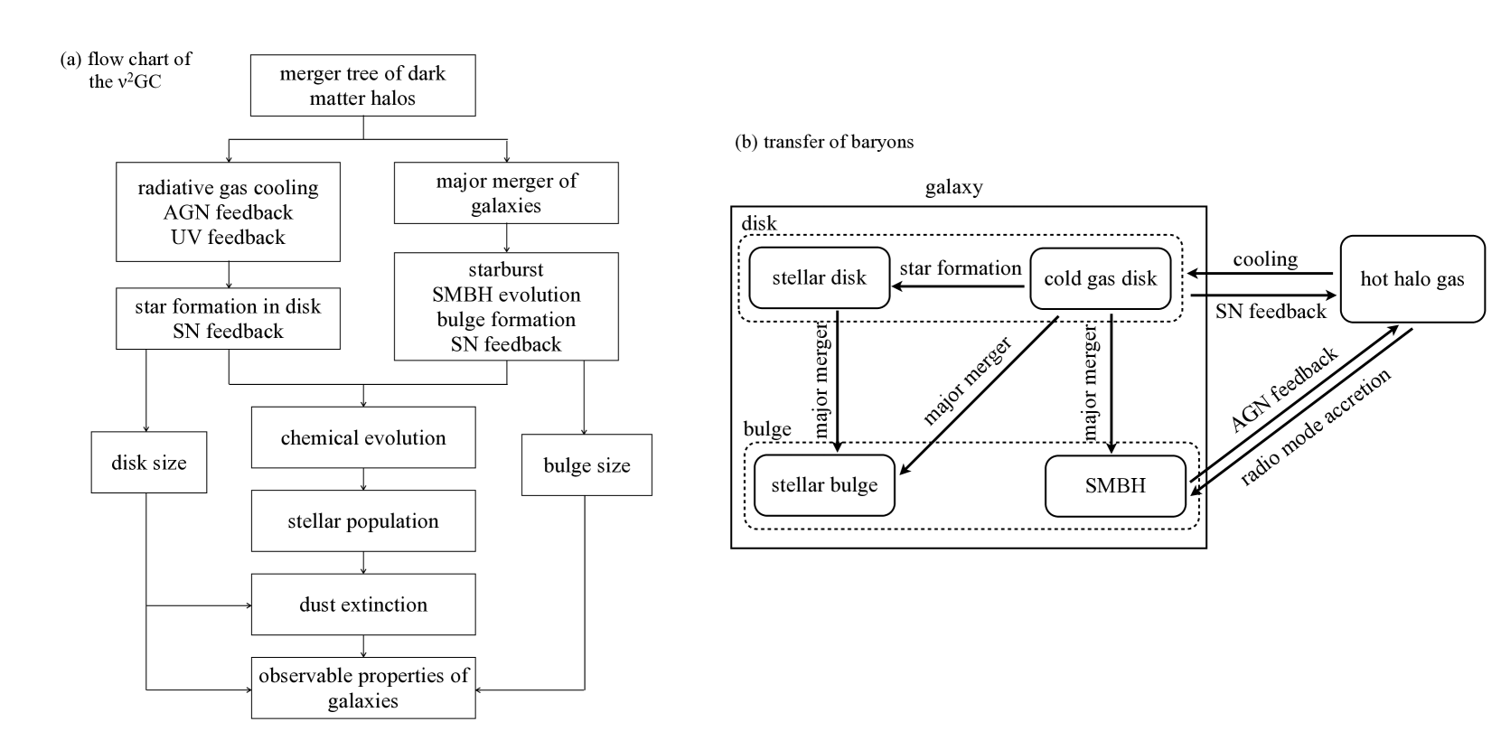
Figure 1: Schematics of the model. (Left) Flow chart of the model showing how the model predicts the observable properties of galaxies. (Right) Schematic of the transfer of baryon components.

2.1 Dark matter merger trees

The merger trees of DM halos are directly extracted from a series of large cosmological N-body simulations, called the $\nu^{2}$GC simulations (Ishiyama et al., 2015). The basic properties of the $\nu^{2}$GC simulations are summarized in table 1. We conducted seven simulations, varying the mass resolution and spatial volume. The largest $\nu^{2}$GC-L run simulated the motions of $8192^{3}$ (550 billion) DM particles in a comoving box of $1.12\,h^{-1}\rm Gpc$. The mass resolution was $2.20\times 10^{8}\,h^{-1}M_{\odot}$, which is the best one among simulations applying boxes larger than $1\,h^{-1}\rm Gpc$. The mass resolution of the run with the smallest box ($\nu^{2}$GC-H2) was $3.44\times 10^{6}\,h^{-1}M_{\odot}$, which is sufficient to resolve small dwarf galaxies. By combining these simulations, we can generate mock catalogs of galaxies and AGNs with unprecedentedly high resolution and statistical power.

The cosmological parameters of the $\nu^{2}$GC simulations were based on the concordance $\Lambda$CDM model consistent with observational results obtained by the Planck satellite (Planck Collaboration et al., 2014). Namely, $\Omega_{0}=0.31$, $\Omega_{b}=0.048$, $\lambda_{0}=0.69$, $h=0.68$, $n_{s}=0.96$, and $\sigma_{8}=0.83$. The $\nu^{2}$GC simulations were conducted by using a massively parallel TreePM code GreeM (Ishiyama et al., 2009, 2012). DM halos are identified by the friends-of-friends (FoF) group finder (Davis et al., 1985), with the linking parameter $b=0.2$. The smallest halos consisted of 40 particles. The spatial positions of the halos were tracked by using those of the most bound particles. It has been known that the properties of halo merger tree are depend on the halo finding algorithm and tree building algorithm (see, e.g., Knebe et al. 2011; Onions et al. 2012; Elahi et al. 2013; Srisawat et al. 2013; Avila et al. 2014; Lee et al. 2014). For further details of the $\nu^{2}$GC simulations and the method for extracting the merger trees, see companion paper, Ishiyama et al. (2015).

Table 1: Details of the $\nu^{2}$GC simulations. N is the number of simulated particles, $L$ is the comoving box size, $m$ is the particle mass resolution, $M_{\rm min}$ is the mass of the smallest halos, the total number of halos, and $M_{\rm max}$ is the mass of the largest halo in each simulations. The smallest halos consist of 40 particles. In the last two columns, values at z=0 are presented except for the $\nu^{2}$GC-H3 simulation, which was stopped at $z=4$.

Name	$N$	$L(h^{-1}\rm Mpc)$	$m(h^{-1}M_{\odot})$	$M_{\rm min}(h^{-1}M_{\odot})$	#Halos	$M_{\rm max}(h^{-1}M_{\odot})$
$\nu^{2}$GC-L	$8192^{3}$	$1120.0$	$2.20\times 10^{8}$	$8.79\times 10^{9}$	$421,801,565$	$4.11\times 10^{15}$
$\nu^{2}$GC-M	$4096^{3}$	$560.0$	$2.20\times 10^{8}$	$8.79\times 10^{9}$	$52,701,925$	$2.67\times 10^{15}$
$\nu^{2}$GC-S	$2048^{3}$	$280.0$	$2.20\times 10^{8}$	$8.79\times 10^{9}$	$6,575,486$	$1.56\times 10^{15}$
$\nu^{2}$GC-SS	$512^{3}$	$70.0$	$2.20\times 10^{8}$	$8.79\times 10^{9}$	$103,630$	$6.58\times 10^{14}$
$\nu^{2}$GC-H1	$2048^{3}$	$140.0$	$2.75\times 10^{7}$	$1.10\times 10^{9}$	$5,467,200$	$4.81\times 10^{14}$
$\nu^{2}$GC-H2	$2048^{3}$	$70.0$	$3.44\times 10^{6}$	$1.37\times 10^{8}$	$4,600,746$	$4.00\times 10^{14}$
$\nu^{2}$GC-H3	$4096^{3}$	140.0	$3.44\times 10^{6}$	$1.37\times 10^{8}$	$44,679,543(z=4)$	$1.15\times 10^{13}(z=4)$

2.2 Gas cooling

We define the formation epoch of the DM halo as the time at which the DM halo mass doubles its mass since the last formation epoch (Lacey & Cole, 1993). At this time, the physical quantities of the halo, such as circular velocity, halo age and mass density are re-estimated. Before reionization of the universe, the mass fraction of the baryonic matter in a collapsing DM halo is given by $\langle f_{\mathrm{b}}\rangle\equiv\Omega_{\rm b}/\Omega_{0}$ (after cosmic reionization, the baryon mass in a halo deviates from $\langle f_{\mathrm{b}}\rangle$; see subsection 2.3). The baryonic matter consists of diffuse hot gas, dense cold gas, stars, and black holes. When a mass of DM halo decreases, diffuse hot gas also decreases at the same ratio with the decrease of DM mass, while a mass of other baryon components does not change.

When a DM halo of circular velocity $V_{\rm circ}$ forms, the contained gas is shock heated to the virial temperature $T_{\rm vir}$ of the halo:

$$T_{\rm vir}=\frac{1}{2}\frac{\mu m_{\rm p}}{k_{\rm B}}V_{\rm circ}^{2},$$ (1)

where $m_{\rm p},k_{\rm B}$ and $\mu$ are the proton mass, Boltzmann constant and mean molecular weight, respectively. Following Shimizu et al. (2002), we assume that the hot gas distributes through the DM halo with an isothermal density profile with a finite core radius:

$$\rho_{\rm hot}(r)=\frac{\rho_{\rm hot,0}}{1+(r/r_{c})^{2}},$$ (2)

where $r_{c}=0.22R_{\rm vir}/c$, and $R_{\rm vir}$ is the virial radius of the host halo. The concentration parameter $c$ is known to be a function of DM halo mass and redshift. We used the analytical formula of $c$ proposed by Prada et al. (2012), which is obtained by fitting cosmological $N$-body simulations. The model of Prada et al. (2012) and Sánchez-Conde & Prada 2014 are consistent with our $N$-body simulations.

After the collapse of a DM halo, the hot gas gradually cools via radiative cooling, forming a cold gas disk at the halo center. Stars born from the condensed cold gas; and a stellar disk and a cold gas disk consist a galaxy (see section 2.4). The rate of gas cooling is calculated following the model proposed by White & Frenk (1991), which is adopted in most SA models. The time scale of radiative cooling, $t_{\rm cool}$, is calculated as

$$t_{\rm cool}(r)=\frac{3}{2}\frac{\rho_{\rm hot}(r)}{\mu m_{\rm p}}\frac{k_{\rm B}T_{\rm vir}}{n_{\rm e}^{2}(r)\Lambda(T_{\rm vir},Z_{\rm hot})},$$ (3)

where $n_{\rm e}(r)$ is the electron density of hot gas at $r$, $Z_{\rm hot}$ is the metallicity of hot gas, and $\Lambda$ is a metallicity-dependent cooling function provided by Sutherland & Dopita (1993). In each time step, the hot gas within the cooling radius cools and accretes onto the central cold gas disk. The cooling radius $r_{\rm cool}(t)$ is defined as the radius at which the cooling time scale is equal to the time elapsed since the halo formation epoch. If the cooling radius exceeds the virial radius $R_{\rm vir}$, we set to $r_{\rm cool}=R_{\rm vir}$. In this case the mass accretion rate of cold gas should be limited by the free fall time, rather than the cooling time. However, we set the time step to be comparable to the dynamical time scale of halo at each epoch, thus this could not cause a serious problem.

We further assumed that the radial profile of hot gas is kept unchanged until the DM halo doubles its mass, allowing the existence of “cooling hole” at the centre of the halo (i.e., no hot gas is distributed at $r<r_{\rm cool}$). This assumption is clearly unphysical, thus the effect on the gas cooling rate should be checked. Monaco et al. (2014) compared their SA model, MORGANA (Monaco et al. 2007), with other SA models and hydrodynamical simulations to test the cooling models. In their model, the cooling radius is treated as a dynamical variables and the gas profile is recomputed in each time step. They also consider the pressure balance between the hot gas and cooled gas, which determines the size of the cooling hole. One of other SA models examined in Monaco et al. (2014) adopts the cooling model of White & Frenk (1991), as well as our model. Monaco et al. (2014) show that the different cooling models adopted in SA models only makes a marginal difference in cooling rate. See also De Lucia et al. (2010) for a test of the cooling models.

As shown in equation (3), the cooling time scale depend on both the temperature and metallicity of the gas. In our model, the chemical enrichment of the hot gas due to the star formation and SN feedback is consistently solved as shown in subsection 2.4.

Note that the above assumption that the hot gas is heated up by shock at collapse of host halos is adopted just for simplicity. In reality, the cooling time scale of hot gas within galactic scale halos is much shorter than their dynamical time scale. Therefore, the hot gas should cool immediately rather than spherically re-distributing throughout the host halos. In any case, because the cooling time scale is very short, almost all the hot gas cools and thus our assumption is expected to work well. For its opposite case, within cluster-scale halos, the cooling time scale is very long owing to the high virial temperature and the AGN feedback. Again the assumption should be good. For the intermediate scale, we might need more sophisticated treatment. Along with the AGN feedback, these process should be improved in future versions of the model.

2.3 Photoionization heating due to an UV background

Intergalactic gas is photo-heated by the cosmological UV radiation field produced by galaxies and quasars. Because the heated gas cannot be accreted by small halos with shallow gravitational potential wells, photo-heating quenches star formation in small galaxies and hence decreases the number densities of dwarf galaxies (e.g., Doroshkevich et al. 1967; Couchman & Rees 1986). The characteristic halo mass $M_{\mathrm{c}}$, below which a halo cannot retain the heated gas, has been investigated by using cosmological hydrodynamic simulations (e.g., Gnedin 2000).

In this context, Okamoto et al. (2008) performed high-resolution cosmological hydrodynamical simulations with a time-dependent UV background radiation field. They found that the redshift evolution of the characteristic mass, $M_{\mathrm{c}}(z)$, is determined by the following factors for each halo: the relation between $T_{\mathrm{vir}}$ and the equilibrium temperature for the gas $T_{\mathrm{eq}}$ at the edge of the halo, at which the density can be approximated as one third of the cosmic mean, and its merging history (see section 4 in Okamoto et al. 2008). They also found that the mass fraction of baryonic matter in halos with mass $M_{\rm h}$ at redshift $z$ is well-fitted by the following formula, originally proposed by Gnedin (2000):

$$f_{\mathrm{b}}(M_{\rm h},z) = \langle f_{\mathrm{b}}\rangle$$ (4)

$$\times\left\{1+(2^{\alpha_{\mathrm{UV}}/3}-1)\left[\frac{M_{\rm h}}{M_{\mathrm{c}}(z)}\right]^{-\alpha_{\mathrm{UV}}}\right\}^{-\frac{3}{\alpha_{\mathrm{UV}}}},$$

where the parameter $\alpha_{\mathrm{UV}}$ controls the rate of decrease of $f_{\mathrm{b}}$ in low-mass halos, here set to $\alpha_{\mathrm{UV}}=2$. While $f_{\mathrm{b}}(M_{\rm h},z)$ equals to $\langle f_{\mathrm{b}}\rangle$ for the halos with $M_{\rm h}\gg M_{\mathrm{c}}(z)$, it goes to zero in proportion to $(M_{\rm h}/M_{\mathrm{c}})^{3}$ for the halos with $M_{\rm h}\ll M_{\mathrm{c}}(z)$. This decrease is attributed to the suppressed accretion of photo-heated baryonic matter onto the halos. This prescription, given by Okamoto et al. (2008), is newly incorporated into our $\nu^{2}$GC model. Although all the above factors that determine $M_{\mathrm{c}}(z)$ are evaluable in our $\nu^{2}$GC model, we simply adopt their resultant $M_{\mathrm{c}}(z)$ itself in order to avoid a relatively large computational cost to obtain $T_{\mathrm{eq}}(\langle f_{\mathrm{b}}\rangle\rho_{\mathrm{vir}}/3)$.

The details how to incorporate the prescription of Okamoto et al. (2008) are as follows. Before reionization, which is assumed to instantaneously occur at $z=z_{\mathrm{reion}}$, all halos contain baryonic matter with a mass fraction of $f_{\mathrm{b}}=\langle f_{\mathrm{b}}\rangle$ regardless of their masses, as described in subsection 2.2. After reionization, the expected baryon fraction $f_{\mathrm{b}}$ of each halo with mass $M_{\rm h}$ that collapsed at $z$, denoted $f_{\mathrm{b}}(M_{\rm h},z)$, is calculated by equation (4) using a fitting formula for $M_{\mathrm{c}}(z)$:

$$M_{\rm c}(z) = 6.5\times 10^{9}$$ (5)

$$\times\exp(-0.604z)\exp{[-(z/8.37)^{17.6}]}~{}h^{-1}~{}M_{\odot}.$$

This fitting formula is derived from the result of simulation of Okamoto et al. (2008) in which the reionization occurs at $z=9.0$. Figure 2 shows $M_{\rm c}$ as a function of redshift. While the minimum halo mass of the lower resolution models ($M_{\rm min}=8.79\times 10^{9}~{}h^{-1}~{}M_{\odot}$) is larger than $M_{\rm c}$, those of the higher resolution models ($M_{\rm min}=1.10\times 10^{9}~{}h^{-1}~{}M_{\odot}$ for the $\nu^{2}$GC-H1 and $M_{\rm min}=1.37\times 10^{8}~{}h^{-1}~{}M_{\odot}$ for the $\nu^{2}$GC-H2, -H3, respectively) are smaller than $M_{\rm c}$ at low redshift. In the halos with mass below $M_{\rm c}$, the gas heating by the UV background affects the properties of galaxies. To mimic this effect, Somerville (2002) also adopt the formulation of Gnedin (2000); however, they assume that $M_{\rm c}(z)$ is given by constant $V_{\rm circ}=50~{}{\rm km}~{}{\rm s^{-1}}$. In figure 2, we also show the redshift evolution of the halo mass with the fixed circular velocity of $V_{\rm circ}=17$, $30$ and $50~{}{\rm km}~{}{\rm s}^{-1}$, respectively. We can see that the behavior of the $M_{\rm c}$ proposed by Okamoto et al. (2008) and the $M_{\rm c}$ given by fixed $V_{\rm circ}$ are significantly different.

In this paper we treat the effect of the gas heating due to the cosmic UV background as follows. For a halo with total baryonic mass (i.e., the sum of the masses of the stars, SMBH, cold gas, and hot gas of all galaxies in the halo) of $M_{\mathrm{b,tot}}\leq f_{\mathrm{b}}(M_{\rm h},z)M$, the baryonic mass of $f_{\mathrm{b}}(M_{\rm h},z)M_{\rm h}-M_{\mathrm{b,tot}}$ is added to the halo as hot gas with temperature of $T_{\mathrm{vir}}$. On the other hand, for the halos with $M_{\mathrm{b,tot}}>f_{\mathrm{b}}(M_{\rm h},z)M_{\rm h}$, an appropriate mass of hot gas is removed from the halo keeping its metallicity unchanged so that the mass fraction of baryon in the halo coincides with $f_{\mathrm{b}}(M_{\rm h},z)$; this prescription mimics photoevaporation by UV background radiation during the reionization. When $M_{\mathrm{b,tot}}-M_{\mathrm{hot}}>f_{\mathrm{b}}(M_{\rm h},z)M_{\rm h}$, we have to reduce the additional cold gas masses in order to the mass fraction of baryon in the halo coincides with $f_{\mathrm{b}}(M_{\rm h},z)$. However cold gas is much denser than hot gas, and may be self-shielded from the UV background radiation. Therefore we assumed that the cold gas component is not affected by the UV heating and allowed such halos to have larger baryon mass than $f_{\rm b}(M_{\rm h},z)M_{\rm h}$. Note that the fraction of such halos is less than $1\%$, thus the treatment of the cold gas in this process does not have significant effects on the results presented in this paper.

Although Okamoto et al. (2008) found that such photoevaporation is important particularly just after the reionization (see middle panel of figure 5 of Okamoto et al. 2008), the effect in our model is assumed to occur for such less-massive halos with $M_{\mathrm{b,tot}}>f_{\mathrm{b}}(M_{\rm h},z)M_{\rm h}$, regardless of their collapsing redshifts when $z\leq z_{\mathrm{reion}}$.

Figure 2: The redshift evolution of the characteristic mass $M_{\rm c}$, below which a halo cannot retain the intergalactic gas due to the heating by the cosmological UV radiation field. The black filled circles show the results of the cosmological hydrodynamical simulations performed by Okamoto et al. (2008). The thick solid line presents the fitting formula described in equation (5). The horizontal dashed lines denote the minimum halo mass of our N-body simulations ($M_{\rm min}=8.79\times 10^{9},1.10\times 10^{9}$ and $3.44\times 10^{8}~{}M_{\odot}$ from top to bottom, respectively). The thin solid lines correspond to the fixed circular velocity $V_{\rm circ}=50$, $30$ and $17$ km s^-1 from top to bottom.

2.4 Star formation and feedback in disk

In this section we describe the star formation in cold gas disk and the reheating of cold gas by SNe. Our implementation follows the standard recipe adopted in other SA models (e.g., Cole et al. 2000).

The cooling process of diffuse hot gas is followed by star formation in the cold gas disk. The star formation rate (SFR), $\psi$, is given by $\psi=M_{\rm cold}/\tau_{\rm star}$, where $M_{\rm cold}$ is the cold gas mass, and $\tau_{\rm star}$ is the time scale of the star formation (SF). We assume that the star formation activity in galaxy disk is related to the dynamical time scale of the disk, $\tau_{\rm d}\equiv r_{\rm d}/V_{\rm d}$, where $r_{\rm d}$ and $V_{\rm d}$ are the disk radius and disk rotation velocity, respectively, defined in subsection 2.8. Thus we adopt the following formula for star formation time scale $\tau_{\rm star}$,

$$\tau_{\rm star}=\varepsilon_{\rm star}^{-1}\tau_{\rm d}\left[1+\left(\frac{V_{d}}{V_{\rm hot}}\right)^{\alpha_{\rm star}}\right],$$ (6)

where $\varepsilon_{\rm star}$, $\alpha_{\rm star}$, and $V_{\rm hot}$ are free parameters. Although the above modeling of the SF time scale well reproduces the several physical properties of observed galaxies as shown later (see section 5), there could be other modeling for the SF time scale. For example, we have examined the model in which the SF time scale depends on the global dust surface density of galaxy, and found that the choice of SF time scale model could have significant effect on the galaxy formation history (Makiya et al., 2014). Although this would be promising for reproducing many aspects of observed galaxies, in this paper, we adopt this kind of standard prescription of star formation for simplicity.

Consequent to supernova explosion, we assume that a fraction of the cold gas is reheated and ejected from galaxy at a rate of ${M_{\rm cold}}/{\tau_{\rm reheat}}$, where the time scale of reheating, $\tau_{\rm reheat}$ is given as follows:

$$\tau_{\rm reheat}=\frac{\tau_{\rm star}}{\beta(V_{d})},$$ (7)

with

$$\beta(V_{d})\equiv\left(\frac{V_{d}}{V_{\rm hot}}\right)^{-\alpha_{\rm hot}},$$ (8)

where $V_{\rm hot}$ and $\alpha_{\rm hot}$ are free parameters.

With the above equations, we obtain the masses of hot gas, cold gas, and disk stars as functions of time (or redshift). The chemical enrichment associated with star formation and SN feedback is treated by extending the work of Maeder (1992). For simplicity, instantaneous recycling is assumed for SNe II, and any contribution from SNe Ia is neglected.

In summary, the baryon evolution during the star formation process is described by the following equations:

$$\dot{M}_{\rm star} = \alpha\psi(t),$$ (9)

$$\dot{M}_{\rm hot} = \beta\psi(t),$$ (10)

$$\dot{M}_{\rm BH} = f_{\rm BH}\psi(t),$$ (11)

$$\dot{M}_{\rm cold} = -(\alpha+\beta+f_{\rm BH})\psi(t),$$ (12)

$$(M_{\rm cold}Z_{\rm cold})\dot{} = [p-(\alpha+\beta+f_{\rm BH})Z_{\rm cold}]\psi,$$ (13)

$$(M_{\rm hot}Z_{\rm hot})\dot{} = \beta Z_{\rm cold}\psi,$$ (14)

where $M_{\rm star}$ and $M_{\rm hot}$ are the masses of stars and hot gas, respectively; $\psi={M_{\rm cold}}/{\tau_{\rm star}}$ is SFR, $Z_{\rm cold}$ and $Z_{\rm hot}$ are the metallicities of cold and hot gases, respectively, and $M_{\rm BH}$ is the mass of the nuclear SMBH. The constant parameter $f_{\rm BH}$ controls the accretion rate of cold gas onto the SMBH during the starburst. In ordinary star formation process in disk, we assume that no cold gas gets accreted by the SMBH (i.e., $f_{\rm BH}=0.0$). The galaxy merger and SMBH evolution will be detailed in later subsections (2.5 and 2.6). The locked-up mass fraction $\alpha$ and chemical yield $p$ are chosen to be consistent with initial mass function (IMF). For the Chabrier IMF (Chabrier 2003), which is adopted in our standard model, $\alpha=0.52$ and $p=1.68$ $Z_{\odot}$.

We can solve these equations analytically as

$$\Delta M_{\rm cold}(t) = M_{\rm cold}^{0}\left\{1-\exp\left[-(\alpha+\beta)\frac{t}{\tau_{\rm star}}\right]\right\},$$ (15)

$$\Delta M_{\rm star}(t) = \frac{\alpha}{\alpha+\beta}\Delta M_{\rm cold}(t),$$ (16)

$$\Delta M_{\rm hot}(t) = \frac{\beta}{\alpha+\beta}\Delta M_{\rm cold}(t),$$ (17)

$$Z_{\rm cold}(t) = Z_{\rm cold}^{0}+p\frac{t}{\tau_{\rm star}},$$ (18)

$$Z_{\rm hot}(t) = \left[M_{\rm hot}^{0}Z_{\rm hot}^{0}+\frac{\beta}{\alpha+\beta}\left\{\frac{}{}\right.\right.$$ (19)

$$\left(\frac{p}{\alpha+\beta}+Z_{\rm cold}(t)\right)\Delta M_{\rm cold}(t)$$

$$-(Z_{\rm cold}(t)-Z_{\rm cold}^{0})M_{\rm cold}^{0}{\left.\left.\frac{}{}\right\}\right]}/M_{\rm hot}(t),\$$

where the $\Delta$ symbol indicates that the variable is incremented or decremented in the current time step. All $\Delta$ variables are defined as positive. The superscript 0 denotes an initial values at the beginning of the time-step (i.e., $t=0$). Note that here we assumed $f_{\rm BH}=0$. For the case of burst-like star formation induced by major merger, see subsection 2.5.

2.5 Mergers of galaxies and formation of spheroids

After the merging of DM halos, the newly formed halo should contain two or more galaxies. The central galaxy in the most massive progenitor halo is designated as the central galaxy of newly formed halo, while the others are regarded as satellite galaxies. These satellite galaxies will fall into the central galaxy by dynamical friction (central-satellite merger). We set the merger time scale due to the dynamical friction as $\tau_{\rm mrg}=f_{\rm mrg}\tau_{\rm fric}$, where $f_{\rm mrg}\sim 1$ is adjustable parameter and $\tau_{\rm fric}$ is the time scale of dynamical friction. If $\tau_{\rm mrg}$ is shorter than the time elapsed since the satellite galaxy enters the common halo, the satellite and central galaxy are merged. We reset this elapsed time to zero when the host halo mass doubles.

For the time scale of dynamical friction, $\tau_{\rm fric}$, we adopt the formulation of Jiang et al. (2008, 2010) which is obtained by fitting to the cosmological $N$-body simulations :

$$\tau_{\rm fric}=\frac{f(\varepsilon)}{2C}\frac{V_{\rm circ}R_{\rm circ}^{2}}{GM_{\rm s}\ln{(1+M_{\rm h}/M_{\rm s})}}$$ (20)

where $C=0.43$ is a constant fitting parameter, $V_{\rm circ}$ is the circular velocity of the common halo, $R_{\rm circ}$ is the radius of the circular orbit of the satellite halo, and $M_{\rm h}$ and $M_{\rm s}$ are the total mass of the host halo and satellite halo, respectively. We simply assumed that $R_{\rm circ}=R_{\rm h}$ where $R_{\rm h}$ is the virial radius of the host halo. The function $f(\varepsilon)=0.90\varepsilon^{0.47}+0.60$ accounts for the dependence of $\tau_{\rm fric}$ on the orbital circularity $\varepsilon$. We set to $\varepsilon=0.5$, which is the average value of $\varepsilon$ estimated by high-resolution $N$-body simulations performed by Wetzel (2011). In our $N$-body simulations we can resolve the satellite halos even after they entered the common halo, and therefore the time scale of dynamical friction can be directly drown from simulations; however, in this paper we adopted simplified formula described above to save the computational time. The effect of this simplification will be examined in a future paper.

The satellite galaxies can randomly collide and merge (satellite-satellite merger). Makino & Hut (1997) conducted an N-body simulation of a system of same mass galaxies. They find that a merger rate, $k_{\rm MH}$, is described by following simple scaling in this situation:

$$k_{\rm MH} = \frac{N}{500}\left(\frac{1~{}\rm Mpc}{R_{\rm h}}\right)^{3}\left(\frac{r_{\rm gal}}{0.1~{}\rm Mpc}\right)^{2}$$ (21)

$$\times\left(\frac{\sigma_{\rm gal}}{100~{}\rm km~{}s^{-1}}\right)^{4}\left(\frac{300~{}\rm km~{}s^{-1}}{\sigma_{\rm halo}}\right)^{3}\mbox{Gyr}^{-1},$$

where $N$, $\sigma_{\rm gal}$, $r_{\rm gal}$ and $\sigma_{\rm halo}$ are the number of satellite galaxies, one-dimensional velocity dispersions of the galaxy, galaxy radius and parent halo, respectively. In our model a satellite galaxy will collide with another satellite galaxy picked out at random, with the probability of $\Delta t\times k_{\rm MH}$, where $\Delta t$ is the time step of the calculation.

We consider two distinct modes for galaxy merger, i.e., major merger and minor merger. If the ratio of baryonic mass (stars, cold gas, hot gas and SMBH mass) of two merging galaxies, $f$ ($<1$), exceeds the critical value $f_{\rm bulge}$, major merger occurs. Major mergers induce burst-like star formations, in which all of the cold gas in the merging system turns into stars and hot gas. The star formation and SN feedback law is the same with the disk star formation (see section 2.4), except for assuming the very short star formation time scale ($\tau_{\rm star}\rightarrow 0$). The bulges and stellar disks of the progenitor completely reform into the bulge component of the new galaxy, together with the stars born during the merger. Note that when applying the SN feedback law, the disk velocity $V_{d}$ is replaced by the velocity dispersion of the new bulge $V_{b}$ (defined in subsection 2.8).

On the other hand, if $f<f_{\rm bulge}$, a minor merger occurs. In this case, stellar and cold gas components of the smaller galaxy are absorbed into the bulge and cold gas disk of the larger galaxy, respectively, with no starburst events.

2.6 Supermassive black holes

Along with the evolution of galaxies, SMBHs at galaxy centers also evolve by the following mechanismas: (1) SMBH coalescence, (2) accretion of cold gas (during a major merger of galaxies), and (3) “radio-mode” gas accretion. Note that we assume a central SMBH in every galaxy. When the galaxies first collapsed, the seed BH have formed with mass $M_{\rm seed}$, which is a tunable parameter.

It has been shown by theoretical studies that a major merger of galaxies can drive substantial gaseous inflows into a galaxy center (e.g., Mihos & Hernquist, 1994, 1996; Barnes & Hernquist, 1996; Di Matteo et al., 2005; Hopkins et al., 2005, 2006). We assume that a fraction of this inflowing cold gas gets accreted by the central SMBH. The mass of cold gas accreted by the SMBH, $\Delta M_{\rm BH}$ is modeled as follows:

$$\Delta M_{\rm BH} = f_{\rm BH}\Delta M_{\rm star,burst},$$ (22)

where $f_{\rm BH}$ is a constant, and $\Delta M_{\rm star,burst}$ is the total mass of stars formed during the starburst. We set $f_{\rm BH}=0.005$ to match the observed relation between masses of host bulges and SMBHs at $z=0$ (see subsection 5.4). The accretion of cold gas triggers the quasar activities. For more detailed model of quasars, see Enoki et al. (2003), Enoki et al. (2014), and Shirakata et al. (2015).

Considering the very short time scale of starburst ($t/\tau_{\rm star}\rightarrow\infty$) assumed here and the mass accretion onto the nuclear SMBH, we solve equations (9)–(14) to obtain the following:

$$\Delta M_{\rm star} = \frac{\alpha}{\alpha+\beta+f_{\rm BH}}M_{\rm cold}^{\rm 0},$$ (23)

$$\Delta M_{\rm hot} = \frac{\beta}{\alpha+\beta+f_{\rm BH}}M_{\rm cold}^{\rm 0},$$ (24)

$$\Delta M_{\rm BH} = \frac{f_{\rm BH}}{\alpha+\beta+f_{\rm BH}}M_{\rm cold}^{\rm 0},$$ (25)

$$\Delta(M_{\rm hot}Z_{\rm hot}) = \frac{\beta}{\alpha+\beta+f_{\rm BH}}$$ (26)

$$\times \left(\frac{p}{\alpha+\beta+f_{\rm BH}}+Z_{\rm cold}^{0}\right)M_{\rm cold}^{0},$$

where $\Delta M_{\rm star}$, $\Delta M_{\rm hot}$, $\Delta M_{\rm BH}$, and $\Delta(M_{\rm hot}Z_{\rm hot})$ are the increasing amount of the stellar mass, hot gas mass, BH mass and the metal mass in the hot gas, respectively, during a starburst. The superscript 0 indicates the total values in the merger progenitors. We again emphasize that all the cold gas is exhausted in our starburst model.

During a merger event, an SMBH also increases its mass via the SMBH–SMBH coalescence. In this paper, we simply assume that SMBHs merge instantaneously right after the merger of their host galaxies, because it is difficult to estimate the time scale of SMBH mergers owing to the existence of many complicated physical processes such as the dynamical friction, stellar distribution, multiple SMBH interaction, and gas dynamical effects (see, e.g., Colpi 2014). As shown in Enoki et al. (2004), the mass growth of SMBHs in our model is mainly due to the gas accretion during major merger, at least, at z $\lesssim$ 1, and therefore therefore the assumption of the instantaneous coalescence does not have significant effects. The other evolution channel, radio-mode gas accretion related to the AGN feedback process, is described next.

2.7 AGN feedback

To reproduce the observed break at the bright end of the luminosity functions (LFs), we introduced the so-called radio-mode AGN feedback process into our model. In this mode, the hot gas accreted by SMBH powers radio jet that injects energy into the hot halo gas, quenching the cooling of the hot gas and resultant star formation in the massive halo. Radio-mode AGN feedback is also expected to contribute to the downsizing evolution of galaxies (e.g., Croton et al., 2006; Bower et al., 2006).

Our implementation of AGN feedback follows the formulation of Bower et al. (2006). In their formulation, gas cooling in the halo is inhibited when the following conditions are satisfied:

$$\alpha_{\rm cool}t_{\rm dyn}(r_{\rm cool})<t_{\rm cool}$$ (27)

and

$$\varepsilon_{\rm SMBH}L_{\rm Edd}>L_{\rm cool},$$ (28)

where $t_{\rm dyn}$ is the dynamical time scale of the halo at the cooling radius, $t_{\rm cool}$ is the time scale of gas cooling, $L_{\rm Edd}$ is the Eddington luminosity of the AGN, $L_{\rm cool}$ is the cooling luminosity of the gas, and $\alpha_{\rm cool}$ and $\varepsilon_{\rm SMBH}$ are free parameters that are tuned to reproduce the observations. Under these conditions, AGN feedback is limited to haloes in quasi-hydrostatic equilibrium, and having a sufficiently evolved SMBH. In the halo experiencing AGN feedback, the SMBH at the center grows by accreting hot halo gas. Bower et al. (2006) assumed that the accretion flow is automatically adjusted by itself so that heating luminosity balances with cooling luminosity, namely, the accretion rate is set to $\dot{M}_{\rm BH}=L_{\rm cool}/\eta c^{2}$. Here $\eta$ is the radiative efficiency. We assumed $\eta=0.1$ for all SMBHs, based on the observational estimation of Davis & Laor (2011). The value of $\eta$ does not significantly affect on the results since the mass growth of SMBHs is dominated by the gas accretion during major merger.

2.8 Size of galaxies and dynamical response to gas removal

This subsection explains how we estimate the galaxy size, disk rotation velocity and velocity dispersion of bulges. Our recipe of size estimation almost follows the procedure of Cole et al. (2000).

2.8.1 Disk formation from cooled gas

First, we estimate the size of galaxy disk as follows. We assume that the hot halo gas has the same specific angular momentum as the DM halo and collapses to the cold gas disk while conserving the angular momentum. We introduce the dimensionless spin parameter $\lambda_{\rm H}$ as $\lambda_{\rm H}\equiv L|E|^{1/2}/GM^{5/2}$, where $L$ is the angular momentum, $E$ is the binding energy and $M$ is the DM halo mass. Although the distribution of $\lambda_{\rm H}$ is often approximated by a log-normal distribution (e.g., Mo et al. 1998), it has been known that the distribution of $\lambda_{\rm H}$ deviates from log-normal in large $N$-body simulations (e.g., Bett et al. 2007). However, according to Bett et al. (2007), the shape of distribution depends on halo finding algorithm and the log-normal function is still slightly better for FoF halos than the modified fitting function proposed by them. In this paper, we simply adopt the log-normal distribution

$$p(\lambda_{\rm H})d\lambda_{\rm H}=\frac{1}{\sqrt{2\pi}\sigma_{\lambda}}\exp\left[-\frac{(\ln\lambda_{\rm H}-\ln\bar{\lambda})^{2}}{2\sigma_{\lambda}^{2}}\right]d\ln\lambda_{\rm H},$$ (29)

where $\bar{\lambda}$ and $\sigma_{\lambda}$ denote the mean and logarithmic variance of the spin parameter, respectively. Here we use $\bar{\lambda}=0.042$ and $\sigma_{\lambda}=0.26$., which are the value obtained by Bett et al. 2007 for FoF halos.

Using the spin parameter $\lambda_{\rm H}$, the effective radius $r_{d}$ of a resultant cold gas disk is expressed as follows (Fall, 1979; Fall & Efstathiou, 1980; Fall, 1983):

$$r_{d}=(1.68/\sqrt{2})\lambda_{\rm H}R_{i},$$ (30)

where the initial radius of the hot gas sphere, $R_{i}$, is set to the virial radius of the host halo or the cooling radius, whichever is smaller. In each time step, the disk size of central galaxies are updated if their disk mass have increased from the previous time step. At this time, we set the disk rotation velocity $V_{d}$ to be the circular velocity of its host halo.

2.8.2 Dynamical response to disk star formation

After the formation of rotationally supported disks, the SN feedback subsequent to disk star formation expels cold gas continuously. As the baryonic mass of galaxies decreases, the gravitational potential well becomes shallower, depending on the mass ratio of baryons to DM within the galactic disk. In response to the variation of the depth of the gravitational potential well, gravitationally bound systems expand and their rotation speed slows down (Yoshii & Arimoto, 1987). We refer to this effect as the dynamical response here. Dwarf galaxies having shallow gravitational potential wells and therefore suffered significant SN feedback are affected more by the dynamical response. Using our SA models taking into account this for starburst, we have shown that this affects the scaling relations of elliptical galaxies especially for dwarfs (Nagashima & Yoshii, 2004; Nagashima et al., 2005). See those papers for the scheme of introducing the dynamical response in SA models. In the present paper, we also apply this effect to disk evolution.

The basic result for disks used here is given by Koyama et al. (2008). At first, we assume a galactic disk within a static DM halo and approximate the density distributions of disks and DM as the Kuzmin disk (Kuzmin, 1952, 1956) and the Navarro-Frenk-White (NFW) profile (Navarro, Frenk & White, 1997), respectively. Then, we consider that the gas mass of disks gradually decreases due to the SN feedback, that is, the so-called adiabatic mass-loss, and that the dynamical response to the gas removal on the disks. The initial radius of cold gas disk is calculated by equation (30). Here we assume that the disk size is determined only by the gravitational potential of the host dark halo, conserving the specific angular momentum of the cooled gas. Although this might be too simple because the central region of galaxies would form dynamically with cooling gas, it should be a good approximation for the outer disk. Thus we take this treatment in this paper as usual.

Here we define ${\cal M}$ and $R$ as ratios of mass and size at a final state relative to those at an initial state, and $z_{i}$ and $z_{f}$ as ratios of baryonic disk size relative to size of dark halos at those states. According to Koyama et al. (2008), we obtain

$${\cal M}=\frac{1}{R}+\frac{q(z_{f})-z_{i}q(z_{i})/z_{f}}{m_{i}},$$ (31)

where $m_{i}$ is the mass ratio of baryons to dark matter at the initial state, and $q(z)$ is a function depending on the distributions of baryons and dark matter. In this case, we cannot obtain an analytic form of $q(z)$. Instead, we expand the above equation around $z=0$ and $R-1\simeq 0$ as

$${\cal M}=\frac{1}{R}+D(R-1),$$ (32)

where

$$D= \frac{c}{m_{i}}\left[\ln(1+c)-\frac{c}{1+c}\right]^{-1}\left[cz_{i}^{2}\left(3+2\ln\frac{cz_{i}}{2}\right)\right.$$ (33)

$$\qquad\left.-\frac{16}{3}c^{2}z_{i}^{3}-c^{3}z_{i}^{4}\left(\frac{33}{8}+\frac{9}{2}\ln\frac{cz_{i}}{2}\right)\right],$$

and $c$ is the concentration parameter described in section 2.2. Note that we take a higher order term of $z_{i}$ for $q(z)$ than that written in equation (A5) in Koyama et al. (2008).

The approximation used here is justified as follows. It is expected that the change in sizes and disk rotation velocities during a time-step is very small because of the quiescent star formation, and that the size of baryonic disks is smaller sufficiently than that of dark halos. These mean $R-1\ll 1$ and $z_{i}\ll 1$. We have checked that these assumptions are indeed validated in our model.

The change of the disk rotation velocity is given by

$$U\equiv\frac{V_{d,f}}{V_{d,i}}=\left[\frac{m_{f}/z_{f}+4f(z_{f})}{m_{i}/z_{i}+4f(z_{i})}\right]^{1/2},$$ (34)

where $f(z)$ is also a function depending on the distributions of baryons and dark matter, similar to $q(z)$. The form of $f(z)$ is shown in equation (A4) in Koyama et al. (2008).

We would like to recall here the well-known results for non-dark matter case, $R=V^{-1}={\cal M}^{-1}$. These relations are obtained by setting $f(z)$ and $q(z)$ to zero. In the opposite limiting case, because dark matter dominates, $q(z)$ becomes much larger. In this case, even if ${\cal M}$ becomes zero, $R$ and $U$ do not vary. This corresponds to the case discussed in Dekel & Silk (1986).

The effect of the dynamical response on the disk shall be discussed in detail in another paper.

2.8.3 Dynamical Response to starburst and spheroidal remnants

The size of the bulge formed in a major merger is characterized by the virial radius of the baryonic component. Applying the virial theorem the total energy in each galaxy is calculated as follows:

$$E_{i}=-\frac{1}{2}[(M_{b,i}+M_{{\rm BH},i})V_{b,i}^{2}+(M_{d,i}+M_{\rm cold})V_{d,i}^{2}],$$ (35)

where $M_{b}$, $M_{\rm BH}$, $M_{d}$ and $M_{\rm cold}$ are the masses of the bulge, central black hole, stellar disk and cold gas disk, respectively, and $V_{b}$ and $V_{d}$ denote the velocity dispersion of the bulge and the rotation velocity of the disk, respectively. The subscript $i=\{0,1,2\}$ indicate the merged galaxy, larger progenitor galaxy and smaller progenitor galaxy, respectively. Furthermore the orbital energy $E_{\rm orb}$ between the progenitors just before the merger is given as follows:

$$E_{\rm orb}=-\frac{E_{1}E_{2}}{(M_{2}/M_{1})E_{1}+(M_{1}/M_{2})E_{2}}.$$ (36)

By energy conservation, we obtain the following:

$$f_{\rm diss}(E_{1}+E_{2}+E_{\rm orb})=E_{0},$$ (37)

where $f_{\rm diss}$ is the fraction of energy dissipated from the system during major merger. The rate of energy dissipation depends on complicated physical processes such as the viscosity and friction due to gas. In this paper, we simply parameterize $f_{\rm diss}$ as follows:

$$f_{\rm diss}=1+\kappa_{\rm diss}f_{\rm gas},$$ (38)

where

$$f_{\rm gas}=\frac{M_{\rm cold}}{M_{\rm star}+M_{\rm cold}+M_{\rm BH}}$$

is the gas mass fraction of the merging system and $\kappa_{\rm diss}$ is a dimensionless parameter. Here we set $\kappa_{\rm diss}=2.0$ to reproduce the distribution of size and velocity dispersion of elliptical galaxies (see section 5.2). There are several studies on this issue by using hydrodynamical simulations and SA models, and it is confirmed that above parameterization of $f_{\rm diss}$ can be a good approximation (see, e.g., Hopkins et al. 2009; Shankar et al. 2013).

We assumed that there remains only the bulge component supported by velocity dispersion just after the merger. Therefore the velocity dispersion and the size of merger remnant can be estimated from following equations,

$$E_{\rm 0}=-\frac{1}{2}M_{{\rm tot},0}V_{b,0}^{2},$$ (39)

and

$$r_{{\rm b},0}=\frac{GM_{\rm tot,0}}{2V_{b,0}^{2}},$$ (40)

where $M_{{\rm tot},0}$ is the total baryonic mass of the merger remnant.

As a consequence of star formation and SN feedback, part of gas removed from galaxies and the mass of the system changes. At this time the structural parameters of galaxies also changes due to the dynamical response. We include this effect into our model adopting the Jaffe model (Jaffe, 1983). In this paper we assume the case of slow (adiabatic) gas removal compared with the dynamical time scale of the system, similar to that for disks. For the case of rapid gas removal, we refer the reader to Nagashima & Yoshii (2003). According to the Nagashima & Yoshii (2003), the effect of dynamical response becomes stronger in the case of non-adiabatic gas removal. Therefore the assumption of the adiabatic gas removal should be considered as conservative. We should keep in mind that the effect might be stronger for dwarf ellipticals having shorter time scale of gas removal compared to giants.

Defining by ${\cal M},R$ and $U$ the ratios of mass, size and velocity dispersion at a final state relative to those at an initial state, the response under the above assumption is approximately given by

$$R \equiv \frac{r_{f}}{r_{i}}=\frac{1+D/2}{{\cal M}+D/2},$$ (41)

$$U \equiv \frac{V_{b,f}}{V_{b,i}}=\sqrt{\frac{{\cal M}/R+Df(z_{f})/2}{1+Df(z_{i})/2}},$$ (42)

where $D=1/y_{i}z_{i}^{2}$, $y$ and $z$ are the ratios of density and size of baryonic matter to those of dark matter. We use equation (36) in Nagashima et al. (2005) for the form of $f(z)$. The subscripts $i$ and $f$ stand for the initial and final states in the mass loss process. Note that $U$ is the ratio of velocity dispersion, different from that for disks. The contribution of dark matter is estimated from the central circular velocity of halos, $V_{\rm cent}$, which is defined below.

2.8.4 Back reaction of dynamical response to dark halos

When galaxies suffer the dynamical response to gas removal caused by the SN feedback, the dark matter within a central region of dark halos hosting the galaxies must also suffer the dynamical response as its back reaction. For simplicity we compute the dynamical response on the dark matter distribution after the computation of the dynamical response on baryons, although they occur simultaneously in reality. Here we ignore the effect of the so-called adiabatic contraction for dark matter during the condensation of cooled gas. This is because the central region of galaxies should form not adiabatically but dynamically. Thus we assume that the cooled gas condenses and relaxes dynamically together with dark matter and is removed adiabatically by the SN feedback affecting the central region of dark halos as the back reaction. This would require detailed research by using hydrodynamic numerical simulations.

Here we focus on the region within the half-mass radius of central galaxies, at which the density of baryons is expected to be comparable to that of dark matter. To take into account this process, we define a central circular velocity of dark halo $V_{\rm cent}$, approximately within the effective radius of the central galaxy. When a dark halo collapses without any progenitors, $V_{\rm cent}$ is set to $V_{\rm circ}$. After that, although the mass of the dark halo grows by subsequent accretion and/or mergers, $V_{\rm cent}$ remains constant or decreases with the dynamical response. When the mass is doubled, $V_{\rm cent}$ is set to $V_{\rm circ}$ again. According to Nagashima & Yoshii (2004) and Nagashima et al. (2005), we assume that $V_{\rm cent}$ is lowered by the dynamical response to mass loss from a central galaxy of a dark halo by SN feedback as follows,

$$\frac{V_{{\rm cent},f}}{V_{{\rm cent},i}}=\frac{M_{f}/2+M_{d}(r_{i}/r_{d})}{M_{i}/2+M_{d}(r_{i}/r_{d})}.$$ (43)

The change of $V_{\rm cent}$ in each time-step is only a few per cent. Under these conditions, the approximation of static gravitational potential of dark matter is valid even during starbursts. This also applies to subhalos. Rigorously speaking, we must assume an isothermal distribution of dark matter, in which the density is proportional to the inverse of $r^{2}$, because the above equation indicates the dynamical response to mass loss within the half-mass radius of central galaxies. In spite of this, this should be good approximation because the NFW profile has a slope $-1$ and $-3$ within and outside the core radius, respectively, which means that we can expect that the effective slope would be approximately $-2$. Of course this expectation is optimistic since we considered the inner region of a halo where a slope is $-1$. However, we need detailed hydrodynamical simulations to know the actual mass profile since the adiabatic contraction due to gas cooling would affect the slope.

Once a dark halo falls into its host dark halo, it is regarded as a subhalo. Because subhalos do not grow in mass in our model, the central circular velocity of the subhalos monotonically decreases. Although the change of $V_{\rm cent}$ during a time-step is small, accumulated change cannot be negligible owing to the monotonicity. Therefore, this affects the time scales of mergers.

The details of the dynamical response are shown in Nagashima & Yoshii (2003, 2004) and Nagashima et al. (2005) for bulges and Koyama et al. (2008) for disks. The effect of the dynamical response is the most prominent for dwarf galaxies of low circular velocity because of the substantial removal of gas due to strong SN feedback (Yoshii & Arimoto, 1987; Nagashima & Yoshii, 2004). If the dynamical response had not been taken into account, velocity dispersions of dwarf ellipticals would have been much larger than those of observations, determined only by circular velocities of small dark halos in which dwarf ellipticals resided. For giant ellipticals, on the other hand, the effect of the dynamical response is negligible because only a small fraction of gas can be expelled due to weak SN feedback. Similarly, for disks, in order to reproduce the observed Tully-Fisher relation, the dynamical response on disks is required. Otherwise, the slope for dwarf spirals becomes different from observed one as shown in Nagashima et al. (2005). This point will be discussed in detail in another paper.

2.9 Photometric properties and morphological identification

Calculating the baryonic processes described in the above subsections, we finally obtain the SF hand metal enrichment histories of each galaxies. From this information, we can calculate spectral energy distribution (SED) of model galaxies by using a stellar population synthesis code of Bruzual & Charlot (2003).

To estimate the extinction of starlight, we first assume that the dust-to-cold gas ratio is proportional to the metallicity of the cold gas; second, we assume that the dust optical depth is proportional to the dust column density. The dust optical depth $\tau_{\rm dust}$ is then calculated as follows: $\tau_{\rm dust}$ is given by

$$\tau_{\rm dust}=\tau_{0}\left(\frac{M_{\rm cold}}{M_{\odot}}\right)\left(\frac{Z_{\rm cold}}{Z_{\odot}}\right)\left(\frac{r_{\rm d}}{\rm kpc}\right)^{-2}$$ (44)

where $r_{\rm d}$ is the effective radius of the galaxy disk and $\tau_{0}$ is a tunable parameter that should be chosen to fit the local observations (such as LFs). The wavelength dependence of optical depth is assumed to follow Calzetti-law (Calzetti et al., 2000). Dust distribution is assumed to obey the slab dust model (Disney et al., 1989) for disks.

In our model, a major merger induces starburst activity, in which all the cold gas turns into stars and hot gas. Therefore, no cold gas and dust exist immediately after the starburst. Hence, the dust optical depth exactly equals to zero and galaxy color becomes too blue compared to the observations. To avoid this problem, we estimate the amount of dust extinction during the starburst as follows. First, we randomly assign the merger epoch within the current time step. Second, we calculate the amount of remaining dust at the end of the time step. At this time, the time scale of gas consumption during the burst is assumed as the dynamical time scale of the merged system, $r_{\rm b}/V_{\rm b}$. The dust geometry is assumed to be the screen model.

The morphological types of model galaxies were determined by the bulge-to-total luminosity ratio in the $B$-band. In this paper we follow the criteria of Simien & de Vaucouleurs (1986): galaxies with B/T $>$ 0.6, 0.4 $<$ B/T $\leq$ 0.6, and B/T $\leq$ 0.4 are classified as elliptical, lenticular, and spiral galaxies, respectively. According to Kauffmann & White (1993) and Baugh et al. (1996), this classification reproduces well the observed type mix.

3 Parameter settings

As described in section 2, our model is constructed from physically motivated prescriptions of several astrophysical processes. However, a number of free parameter remain. Here we describe the parameter setting procedure.

3.1 Overview of parameter settings

For the cosmological parameters, we adopt the Planck cosmology (Planck Collaboration et al., 2014). The several free parameters related to astrophysical processes are listed in table 2. Seven of these parameters, namely, $\alpha_{\rm star}$, $\tau_{\rm star}$, $\alpha_{\rm hot}$, $V_{\rm hot}$ $\alpha_{\rm cool}$, $\varepsilon_{\rm SMBH}$ and $M_{\rm seed}$ were tuned to fit the local optical ($r$-band) and near IR ($K$-band) LFs and the local mass function (MF) of cold neutral hydrogen, by using a MCMC method (see next section). We use the local LFs and HI MF as the fiducial references in model calibration, since they are robustly determined from recent large and deep surveys. The other parameters, $f_{\rm bulge}$, $f_{\rm mrg}$, $f_{\rm BH}$, $\tau_{V0}$ and $\kappa_{\rm diss}$, are manually tuned by comparing other observations, since they cannot be constrained by the local LFs and HI MF.

The galaxy merger-related parameters, $f_{\rm bulge}$ and $f_{\rm mrg}$, are closely related to the abundance of elliptical galaxies, hence they can be constrained by the LFs divided by morphological class. However there are still some uncertainties in the determination of morphology, thus we did not use them in the fitting. In this paper we simply assumed that $f_{\rm bulge}=0.1$ and $f_{\rm mrg}=0.8$, which is the same value with N05. The mass fraction accreted by SMBH during a starburst, $f_{\rm BH}$, affects the bright-end shape of LFs through the AGN feedback; however it is degenerated with other AGN feedback-related parameters, $\varepsilon_{\rm SMBH}$ and $M_{\rm seed}$, and is poorly constrained by LFs. Thus we tuned $f_{\rm BH}$ to reproduce the observed BH mass – bulge mass relation and mass function of SMBHs, which are significantly affected by $f_{\rm BH}$ but not by other two parameters. We have found that $f_{\rm BH}=0.005$ is suitable to reproduce the observations in the case of $f_{\rm bulge}=0.1$ and $f_{\rm mrg}=0.8$ (see section 5.4). The coefficient of dust extinction, $\tau_{V0}$, was set to the value adopted in N05, namely $\tau_{V0}=2.5\times 10^{-9}$. The parameter related to the energy loss fraction in a major merger ($\kappa_{\rm diss}=2.0$) was chosen to fit the size–magnitude relation of elliptical galaxies (see section 5). Throughout this paper, we adopt the Chabrier IMF in the mass range 0.1–100 $M_{\odot}$.

Although the MCMC method is numerically economical, it still requires approximately $\sim 10^{5}$ realizations to estimate the reliable parameter range. Therefore, to restrain the runtime of each realization within a few seconds, we employed the $\nu^{2}$GC–SS model for the $N$-body data in the MCMC fitting, which has the lowest mass resolution and the smallest box size. The mass resolution of $N$-body data could have complicated effects on the merging history of DM halos, thus there is no guarantee that the parameters tuned for $\nu^{2}$GC–SS model work well for other $N$-body runs. However no significant differences between the $\nu^{2}$GC-SS and $\nu^{2}$GC–H2 (the highest resolution model) are found in the $r$- and $K$-band LFs and HI MF in the magnitude and mass range used in the fitting (see section 3.4 and figure 4, 5).

3.2 Markov chain Monte Carlo analysis

MCMC analysis was implemented by the Metropolis–-Hastings algorithm (Metropolis et al. 1953; Hastings 1970), which is the most commonly used MCMC method. This method requires the proposal distribution $q$, which suggests a candidate point for the next step, given the previous sampling point. We assume a Gaussian distribution function for $q$. The variance of the Gaussian function is manually selected, to decrease the convergence time. We run 8 MCMC chains in parallel from random starting points. Each chain has about 50,000 realizations, excluding initial 10,000 steps of ”burn-in” phase. The convergence of MCMC chain is checked by the Gelman-Rubin diagnostic test (Gelman & Rubin 1992). In this method, the difference between the multiple MCMC chains are quantified by the ratio of the variance between chains to the variance within chain, $\hat{R}$. In this paper the chain is considered to have converged when $\hat{R}<1.1$. As a result of the fitting, all the free parameters examined here reach convergence. We simply assume the uniform distribution for the prior probability distribution, with the range listed in table 2. Although the bounds of prior distributions are physically chosen, the ranges are set to be wide in order to cover a large model space, since our knowledge about the posetrior distribution of parameters is limited.

3.3 Observational data and error estimation

In this subsection, we describe the observational data used in the MCMC fitting. The local $r$- and $K$-band LFs were obtained by the Galaxy and Mass Assembly (GAMA) survey (Driver et al., 2012), and HI MF was extracted from the data of the Arecibo Legacy Fast ALFA (ALFALFA) survey (Martin et al., 2010).

For each realization, the likelihood is calculated as follows:

$$\mathcal{L}=\mathcal{L}_{0}\exp\left(-\frac{\chi^{2}_{r}+\chi^{2}_{K}+\chi^{2}_{\rm H\emissiontype{I}}}{2}\right),$$ (45)

where $\mathcal{L}_{0}$ is an arbitrary constant and $\chi_{r}$, $\chi_{K}$ and $\chi_{\rm H\emissiontype{I}}$ are the $\chi^{2}$ values of the $r$-band LF, $K$-band LF and HI MF, respectively. These values are estimated as follows:

$$\chi^{2}(\phi_{\rm obs}|\theta)=\sum_{i}\frac{\{\phi_{i,{\rm obs}}-\phi_{i,{\rm model}}(\theta)\}^{2}}{\sigma_{i,{\rm obs}}^{2}+\sigma_{i,{\rm model}}(\theta)^{2}}$$ (46)

where $\phi_{i,{\rm obs}}$ denotes the value in the $i$th bin of the observed LF (or HI MF), $\phi_{i,{\rm model}}(\theta)$ is the value of the model in the $i$th bin obtained with the parameter set $\theta$ and $\sigma_{i,{\rm obs}}$ and $\sigma_{i,{\rm model}}$ are the errors in the observation and model in each bin, respectively. The errors in the observed LFs only include Poisson errors (Driver et al. 2012), while the errors in the observed HI MF include the systematic errors in mass estimation in addition to Poisson errors.

The errors in the model predictions, $\sigma_{i,{\rm model}}$, were assumed as the sum of Poisson statistical errors and systematic errors coming from cosmic variance. Although the most of SA models assume Poisson errors for the model (e.g., Henriques et al. 2009; Lu et al. 2014), it is controversial whether this assumption is appropriate or not. However typical value of Poisson errors are less than $1\%$ of the error coming from the cosmic variance described below, it does not have significant effect on the parameter fitting. Although the errors of the observed HI MF include the systematic errors come mainly from uncertainty of mass estimation, especially for low HI mass galaxies (see, e.g., Zwaan et al. 2005; Martin et al. 2010), we does not include it in the errors of our model.

The effect of cosmic variance is estimated as follows. First, we ran the model using the $\nu^{2}$GC-S for the N-body data, which has a larger box ($L=280h^{-1}$ Mpc) than that in the MCMC fitting ($L=70h^{-1}$ Mpc), and randomly picked out the $L=70h^{-1}$ Mpc box from the large box data in $\sim$100 trials. Following this, we drew the LFs and HI MF from the small boxes and determined their uncertainties (approximately 20%) in each bin. We accounted for this 20% uncertainty in $\sigma_{i,{\rm moodel}}$, in addition to Poisson errors.

Populations of dwarf galaxies with low surface brightness are known to exist, and the faint-end slope of observed LFs may be affected from the surface brightness limits of galaxy surveys (e.g. Blanton et al. 2005). According to Baldry et al. (2012), the incompleteness of GAMA samples become larger than 30% at $\mu_{r,50}\gtrsim$ 23.5 mag ${\rm arcsec}^{-2}$, where $\mu_{r,50}$ is the surface brightness within the Petrosian half-light radius. Therefore, we adopt this limit in calculating the model LFs. To calculate the Petrosian surface brightness, we require the light profile of galaxies. However, because our model does not resolve the internal structure of galaxies, we converted the effective radius and total magnitude into the Petrosian radius and Petrosian magnitude, respectively, fixing the Sérsic index $n_{\rm s}$ of bulge ($n_{\rm s}=4$) and disk ($n_{\rm s}=1$) components for all galaxies.

The mass of cold atomic hydrogen of model galaxies are estimated as follows. First we assume that the 75% of the cold gas is composed of hydrogen. This cold hydrogen will be split into atomic and molecular; however, our current model does not follow the complex history of the formation of molecular hydrogen. Therefore we simply assume a fixed $\mathrm{H}_{2}$-to-HI ratio for all galaxies. According to the observational estimation of Keres et al. (2003) and Zwaan et al. (2005), a global mass ratio of molecular to atomic hydrogen is $\sim 0.4$. Thus the mass of cold atomic hydrogen is estimated as

$$M_{\rm H\emissiontype{I}}=0.75/(1+0.4)M_{\rm cold}.$$ (47)

Note that similar approach was used in other SA models (e.g. Power et al. 2010; Lu et al. 2012). When fitting HI MF, we only used the data points acquired at $M_{\rm H\emissiontype{I}}>10^{8}M_{\odot}$, because at masses below this limit, the mass resolution the N-body data would affect the shape of low mass end of HI MF (see next subsection). The uncertainties in the observed HI MF also increase below this limit due to the incompleteness of the survey (Martin et al. 2010).

3.4 Fitting results

The diagonal panels of figure 3 present the 1D posterior probability distributions of the parameters tuned in the MCMC fitting. From the 1D posterior probability distributions, we computed the medians and 10 and 90 percentiles of each parameter; the statistics are summarized in table 2. The off-diagonal panels of figure 3 present the 2D posterior probability distributions of all combinations of the seven free model parameters (grey contours). The 1D distributions of the five parameters, $\alpha_{\rm star}$, $\tau_{\rm star}$, $\alpha_{\rm hot}$, $V_{\rm hot}$, and $\alpha_{\rm cool}$ are highly-peaked, indicating that they are well constrained within the assumed range. On the other hand, $\varepsilon_{\rm SMBH}$ and $M_{\rm seed}$ have broad distribution. This can be understood as follows. If these parameters are large enough, the second condition of AGN feedback [equation (28)] will be satisfied in all halos. In such case, the specific value of these parameters no longer affect the shape of LFs and MF, and therefore only the lower boundary of these can be constrained from the fitting of LFs and HI MF. The posterior distribution of $M_{\rm seed}$ suggests that the $M_{\rm seed}$ should be larger than $10^{5}M_{\odot}$. This seed BH mass is somewhat higher than other SA models. In our model a fraction of central galaxies is bulge-less (i.e. they have never experience any major merger event till $z=0$). The SMBH mass is equal to $M_{\rm seed}$ in such galaxies, thus large value of $M_{\rm seed}$ is required in order to make AGN feedback work in such halos.

Figure 4 present the $r$- and $K$-band LFs in the model with the MCMC-obtained best fit parameters. The model closely matches the observations over all magnitude ranges. The shaded regions indicate the $1\sigma$ error in the model LFs, estimated from the $1\sigma$ confidence interval of each parameter. To see the effect of the mass resolution, we also plot the results of $\nu^{2}$GC-H2 model with the same parameters. These models are consistent within the $1\sigma$ error.

Figure 5 shows HI MF computed by the best-fit model. Data below the lower limit of the HI mass (solid vertical line) were excluded in the MCMC fitting because they deviated when the model was run at higher mass resolution ($\nu^{2}$GC-H2 model, $M_{\rm min}=1.37\times 10^{8}h^{-1}M_{\odot}$; dashed line). Although there remains uncertainties in both the model and the observation, the model seems to underpredict the abundance of lower HI mass galaxies ($M_{\rm H\emissiontype{I}}<10^{8}M_{\odot}$). The similar trend is seen in other SA models. For example, Gonzalez-Perez et al. (2014) find that their model also underpredicts the abundance of galaxies at the lower-mass end of HI MF (see also Lagos et al. 2014). They conclude that this is mainly due to the limited mass resolution of their N-body data. However, even in the $\nu^{2}$GC-H2 model, which has approximately two orders of magnitude higher mass resolution than that of Gonzalez-Perez et al. (2014), the lower-mass end of the HI MF is still underpredicted. This result might suggest that the more realistic modeling of star formation and SN feedback is required (e.g., Lu et al. 2014; Benson 2014). Furthermore, non-virialized gas which is not included in our model and/or HI gas with low HI column densities below the observation limits of the current HI blind surveys might contribute to the low end of the  HI MF (e.g., Okoshi et al. 2010). We will further investigate this issue in the future.

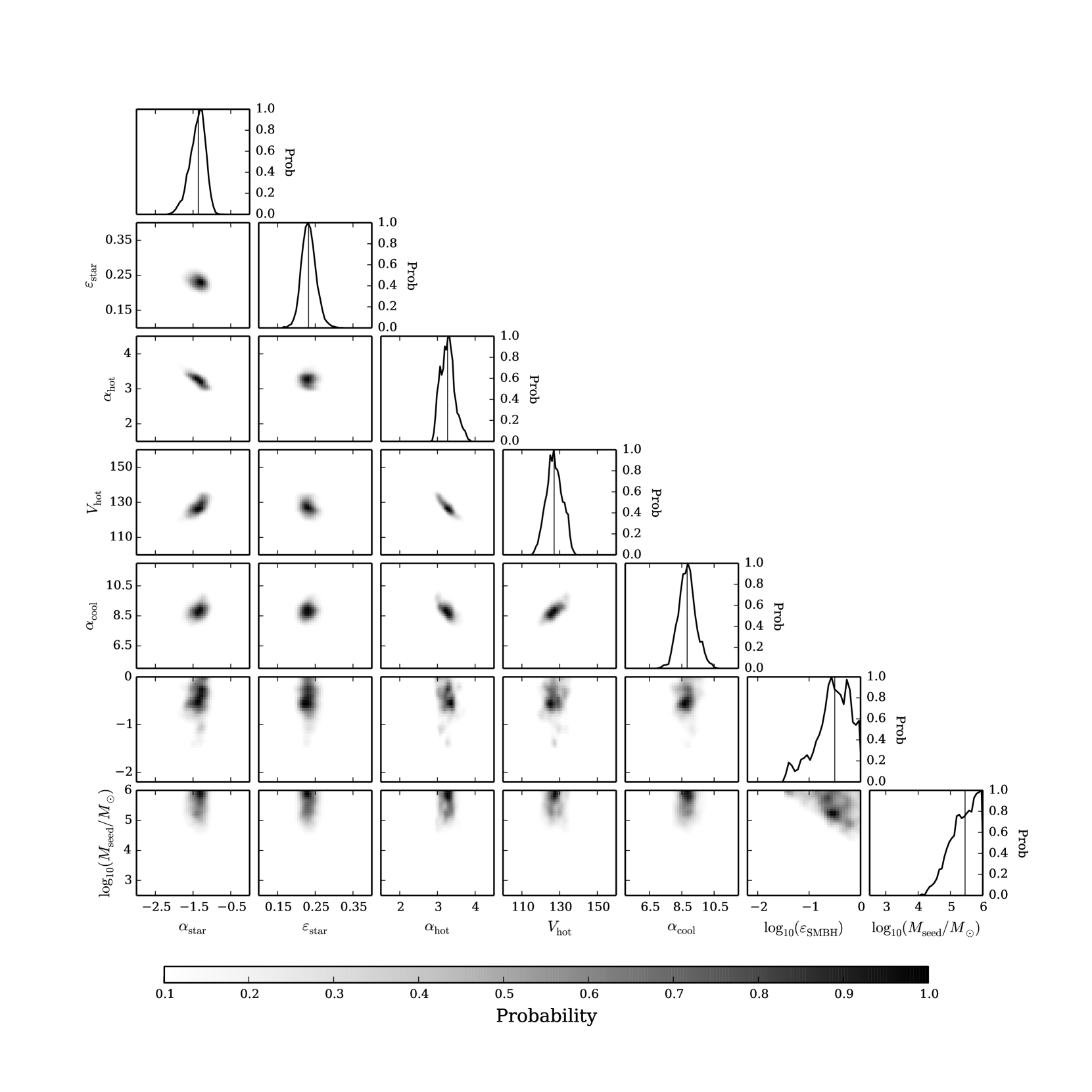
Figure 3: The 1D (diagonal panels) and 2D (off-diagonal panels) posterior probability distribution functions of five free parameters tuned in MCMC fitting. The solid vertical lines in diagonal panels show the median of each distribution. Probability distributions of all combinations of the five parameters are shown by grey contours.

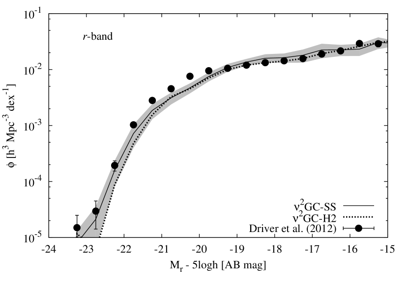
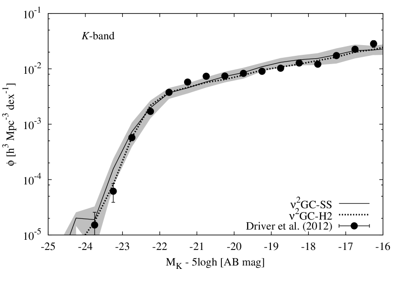
Figure 4: The $r$- and $K$-band LFs. The black solid line represents the model ($\nu^{2}$GC-SS) with the best-fit parameters determined by MCMC fitting. The black dotted line shows the model with the same parameters but using the high-resolution N-body data ($\nu^{2}$GC-H2). The shaded region denotes the $1\sigma$ error in the model, estimated from the posterior probability distribution of the parameters (figure 3). The observational data shown in black filled circles are obtained by GAMA survey (Driver et al. 2012).

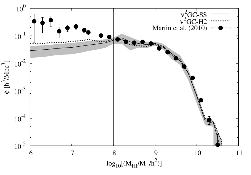
Figure 5: HI mass function of the best fit model. The black solid line represents the model ($\nu^{2}$GC-SS) with the best-fit parameters determined by MCMC fitting. The black dotted line shows the model with the same parameters but using the high-resolution N-body data ($\nu^{2}$GC-H2). The mass resolution of N-body data would affects the shape of MF below $M_{\rm H\emissiontype{I}}\sim 10^{8}M_{\odot}$ (shown by vertical solid line); therefore, data below this were excluded in the parameter fitting. The shaded region denotes the $1\sigma$ error in the model, estimated from the posterior probability distribution of the parameters (figure 3). Black filled circles are the observational data obtained by ALFALFA survey (Martin et al. 2010).

Table 2: The list of free parameters related to astrophysical processes. Seven of these parameters, namely, $\alpha_{\rm star}$, $\tau_{\rm star}$, $\alpha_{\rm hot}$, $V_{\rm hot}$, $\alpha_{\rm cool}$, $\varepsilon_{\rm SMBH}$, and $M_{\rm seed}$were tuned to fit the local LFs and HI MF, by using a MCMC method. See text for details of parameter settings.

		Posterior
	Prior	Median	10 to 90 percentile	Meaning
$\alpha_{\rm star}$	[-5.0, 0.0]	-1.36	[-1.14, -1.67]	star formation-related
$\varepsilon_{\rm star}$	[0.01, 1.0]	0.23	[0.21, 0.26]	star formation-related
$\alpha_{\rm hot}$	[0.0, 5.0]	3.27	[3.03, 3.52]	SN feedback-related
$V_{\rm hot}$ (km/s)	[50.0, 200.0]	127.1	[121.6, 133.1]	SN feedback-related
$\alpha_{\rm cool}$	[0.1, 10.0]	8.83	[8.16, 9.55]	AGN feedback-related
$\log_{10}(\varepsilon_{\rm SMBH})$	[-2.0, 0.0]	-0.50	[-1.02, -0.14]	AGN feedback-related
$\log_{10}(M_{\rm seed}/M_{\odot})$	[3.0, 6.0]	5.45	[4.83, 5.90]	seed black hole mass
$f_{\rm BH}$	–	$5\times 10^{-3}$ (fix)	–	fraction of the mass accreted onto SMBH
				during major merger
$\tau_{V0}$	–	$2.5\times 10^{-9}$ (fix)	–	coefficient of dust extinction
$f_{\rm bulge}$	–	0.1 (fix)	–	major/minor merger criterion
$f_{\rm mrg}$	–	1.0 (fix)	–	coefficient of dynamical friction time scale
$\kappa_{\rm diss}$	–	2.0 (fix)	–	energy loss fraction

4 Numerical galaxy catalog

Following the above procedures, we finally obtained the numerical galaxy catalog. This catalog contains various data on each mock galaxies: redshift, three-dimensional positions, physical quantities such as stellar mass, gas mass, metallicity, star formation rate, effective radius, and magnitudes in several passbands in the UV–NIR regime. More information is provided at here.

Figure 6 plots the spatial distribution of the model galaxies from $z=0.0$ to $z=11.6$ (corresponding to approximately $10^{4}$ Mpc along the comoving radial distance), plotted on the past light-cone of an observer at $z=0$. Here we show the result of the $\nu^{2}$GC-H1 model. The light-cone is generated by patchworking the model outputs at various redshift slices. During the patchworking, the simulation box was randomly shifted and rotated to avoid artifacts in the spatial structure. Web-like structures are clearly visible in this figure. Thanks to the high mass resolution of the model, we can observe galaxies even at $z>10$.

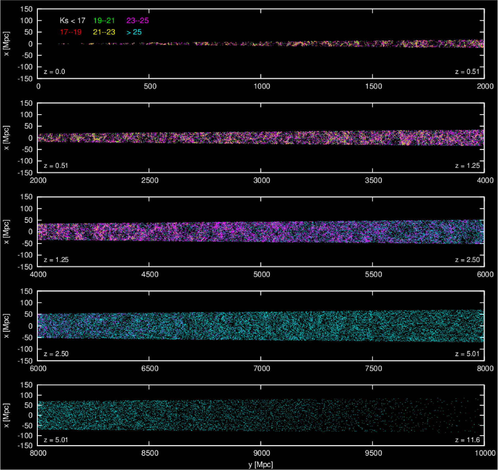
Figure 6: The spatial distribution of the mock galaxies plotted on the past light-cone of an observer located at redshift zero. The color indicates the apparent magnitude of each galaxies in the 2MASS Ks-band. We only show the one-thousandth of galaxies which are randomly picked up from total sample, to avoid a confusion.

5 Local galaxies

In this section we compare the model predictions with local observations. In what follows, we show the results of the $\nu^{2}$GC-H2 model which has the highest mass resolution, unless otherwise mentioned. The adopted parameters related to the baryon physics are listed in table 2.

5.1 Size and disk rotation velocity of spiral galaxies

First, we compare the predicted effective radius and disk rotation velocity of spiral galaxies with the observations. For the observational data, we use the data taken from Courteau et al. (2007). The sample of Courteau et al. (2007) is a compilation of the major samples of local spiral galaxies for which rotational velocities are available. Their sample includes Mathewson et al. (1992), Dale et al. (1999), Courteau et al. (2000), Tully et al. (1996) and Verheijen (2001). The disk scale length of the sample galaxies are estimated from the $I$-band image, and the disk rotation velocities are estimated from H$\alpha$ or HI line widths. Both of the disk size and the rotation velocity are corrected for inclination.

Figures 7 and 8 show the scaling relations between the effective disk radius and the $I$-band magnitude, and between the disk rotation velocity and the $I$-band magnitude (the so-called Tully-Fisher relation; Tully & Fisher 1977), respectively. The median and the 10th to the 90th percentile of the distribution of model galaxies in each magnitude bin are shown by black squares with error bars. The observational data are shown by small gray dots. The model very well reproduces these observed scaling relations over all magnitude range. The effect of the dynamical response to the disk will be investigated in detail in future paper.

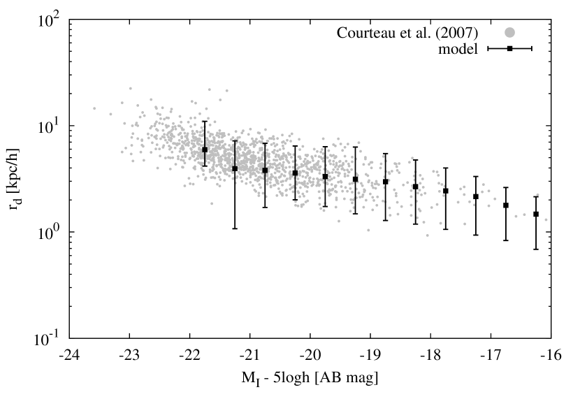
Figure 7: Effective radius of spiral galaxies plotted against $I$-band magnitude. The black filled squares with error bars show the median and the 10th to the 90th percentile of the predicted size of model galaxies in each magnitude bin. Small gray dots are the observational data obtained by Courteau et al. (2007).

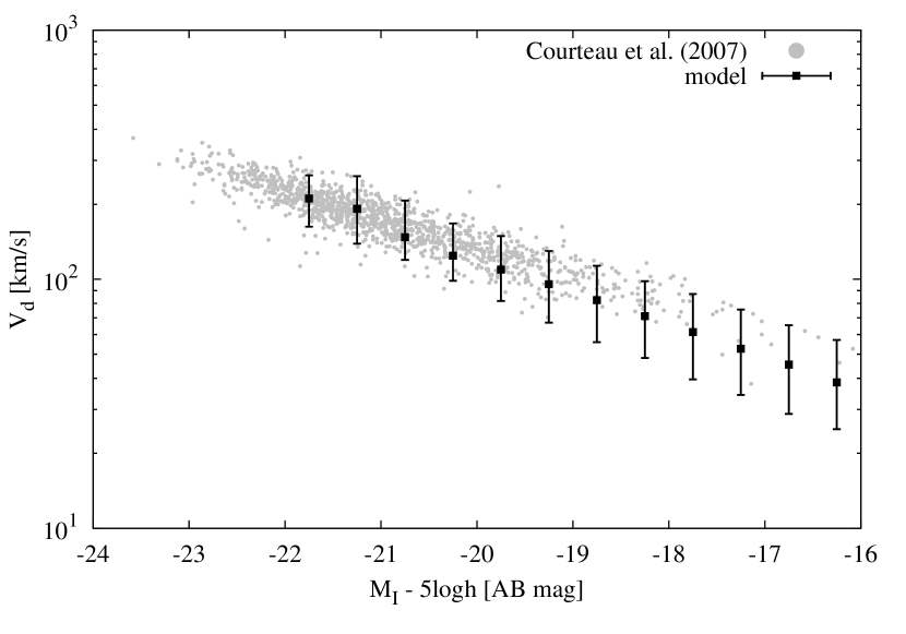
Figure 8: $I$-band Tully-Fisher relation (i.e., disk rotation velocity against $I$-band magnitude) of spiral galaxies. The black filled squares with error bars show the median and the 10th to the 90th percentile of the predicted disk velocity of model galaxies in each magnitude bin. Small gray dots are the observational data obtained by Courteau et al. (2007).

5.2 Size and velocity dispersion of elliptical galaxies

In this subsection we compare the predicted effective radius and velocity dispersion of elliptical galaxies with the observations. For the observational data, we use the data compiled by Forbes et al. (2008). They take the central velocity dispersions of sample galaxies from the catalog of Bender & Nieto (1990), Bender et al. (1992), Burstein et al. (1997), Faber et al. (1989), Trager et al. (2000), Moore et al. (2002), Matković & Guzmán (2005) and Firth et al. (2007). The half-light radii are calculated from 2MASS $K$-band 20th isophotal size, by using a empirical relation based on Sérsic light profiles (Forbes et al. 2008).

Figures 9 and 10 show the scaling relations between the effective radius and the $K$-band magnitude, and between the velocity dispersion and the $K$-band magnitude (the so-called Faber-Jackson relation; Faber & Jackson 1976), respectively. The median and the 10th to the 90th percentile of the distribution of model galaxies in each magnitude bin are shown by black squares with error bars. The effective radius of model galaxy, $r_{e}$, is estimated from $r_{e}=0.744r_{b}$ (Nagashima & Yoshii, 2003), where $r_{b}$ is the three-dimensional half-mass radius. The projected velocity dispersion is estimated as $\sigma_{\rm 1D}=V_{\rm b}/\sqrt{3}$ after being increased to the central value by a factor of $\sqrt{2}$ assuming the de Vaucouleurs profile.

As shown in figures 9 and 10, our model underpredicts both of the size and the velocity dispersion of galaxies brighter than $M_{\rm K}\sim-20$, comparing with the observations. The size and velocity dispersion are related to the dynamical mass of a galaxy as $M_{\rm dyn}\propto r_{\rm e}^{2}V_{\rm b}$, and therefore the model also underpredicts the dynamical mass of bright elliptical galaxies at a fixed magnitude. These results might imply that our treatment of bulge (and elliptical galaxies) formation process is oversimplified. We need to consider more realistic model for galaxy merger, as well as another channels of bulge formation such as disk instabilities. Furthermore, assumed IMF might also be responsible for the underprediction of mass-to-luminosity ratio.

Figure 9: Effective radius of elliptical and lenticular galaxies plotted against $K$-band magnitude. The black filled squares with error bars show the median and the 10th to the 90th percentile of the predicted size of model galaxies in each magnitude bin. Small gray dots are the observational data estimated by Forbes et al. (2008).

Figure 10: $K$-band Faber-Jackson relation (i.e., projected central velocity dispersion against $K$-band magnitude) of elliptical and lenticular galaxies. The black filled squares with error bars show the median and the 10th to the 90th percentile of the distribution of predicted velocity dispersion of model galaxies in each magnitude bin. The projected velocity dispersion of model galaxies are estimated as $\sigma_{\rm 1D}=V_{\rm b}/\sqrt{3}$ after being increased to the central value by a factor of $\sqrt{2}$ assuming the de Vaucouleurs profile. Small gray dots are the observational data compiled by Forbes et al. (2008).

5.3 Cold gas

Figure 11 presents the cold atomic hydrogen mass relative to the $r$-band luminosity against the $r$-band magnitude for local spiral galaxies. As described above, the atomic hydrogen mass of model galaxy is estimated as $M_{\rm H\emissiontype{I}}=0.54M_{\rm cold}$ (see section 3.3). The median and the 10th to the 90th percentile of the distribution of model galaxies in each magnitude bin are shown by black squares with error bars. The observational data shown in small gray dots are taken from ALFALFA 40% catalog ($\alpha.40$; Haynes et al. 2011).

As already mentioned above, the uncertainties in the model increase for galaxies having HI mass less than $10^{8}M_{\odot}$ (see section 3.3). Furthermore, the $\alpha.40$ catalog is highly incomplete for galaxies at $M_{\rm H\emissiontype{I}}<10^{8}M_{\odot}$ (Haynes et al. 2011). Therefore we only plot galaxies having $M_{\rm H\emissiontype{I}}>10^{8}M_{\odot}$ for both of the model and the observation. The diagonal solid line in figure 11 corresponds to $M_{\rm H\emissiontype{I}}=10^{8}M_{\odot}$.

We can see that the model very well reproduces the observation over all magnitude range. The cold gas mass to luminosity ration is mainly determined by the balance of gas consumption rate by star formation and SN feedback. The agreement between the model and observation seen in figure 11 supports the validity of our model of star formation and SN feedback. For more detailed discussion on the properties of cold gas component in our model, we refer the reader to Okoshi & Nagashima (2005) and Okoshi et al. (2010) although they are based on our previous model.

Figure 11: Cold gas mass relative to $r$-band luminosity as a function of $r$-band magnitude for spiral galaxies. Small gray dots are the observational data obtained by 40% catalog of ALFALFA survey ($\alpha.40$; Haynes et al. 2011). Here we only show the galaxies having HI mass greater than $10^{8}M_{\odot}$. The solid diagonal line corresponds to the constant hydrogen mass of $M_{\rm H\emissiontype{I}}=10^{8}M_{\odot}$. The black filled squares with error bars show the median and the 10th to the 90th percentile of distributions of the model galaxies in each magnitude bin. We simply estimated the mass of cold atomic hydrogen as $M_{\rm H\emissiontype{I}}=0.54M_{\rm cold}$ (see text for detail).

5.4 Supermassive black holes

In this subsection we present the properties of SMBHs at local universe. Figure 12 shows the predicted relation between the bulge mass and the SMBH mass, comparing with the observational data obtained by McConnell & Ma (2013). To show the distribution of more massive and rarer objects, we also plot the $\nu^{2}$GC-M model in this figure. With a fixed mass fraction of cold gas accreted by a SMBH during a starburst ($f_{\rm BH}=0.005$), the observed relation is naturally explained by the model. However $f_{\rm BH}$ degenerates with other parameters which are related to bulge formation and SMBH evolution, such as $f_{\rm bulge}$ and $f_{\rm mrg}$, and therefore we need another observational constraints to discuss the physical meanings of these parameters. For example, morphology-dependent LFs will help to resolve the degeneracy since $f_{\rm bulge}$ and $f_{\rm mrg}$ control the abundance of bulge component. Gravitational waves from SMBHs will also provide us strong and independent constraints (see, e.g., Enoki et al. 2004; Enoki & Nagashima 2007). Figure 13 show the predicted MF of local SMBHs, comparing with the observational estimation by Shankar et al. (2004). The model also well reproduces the observation over all mass range.

For more detailed discussions on the properties of AGN populations, see Enoki et al. (2003), Enoki et al. (2014) and Shirakata et al. (2015), although they are based on our previous model.

Figure 12: The SMBH mass versus bulge mass relation. The black filled squares with error bars show the median and the 10th to the 90 percentile of the distribution of model galaxies in each bin of bulge mass for the $\nu^{2}$GC-H2 model. The crosses are the results of $\nu^{2}$GC-M model, which is shifted about $+0.05$ dex in $\log(M_{\rm bulge}/M_{\odot})$ to avoid a confusion. The observational data obtained by McConnell & Ma (2013) are shown by open circles.

Figure 13: The mass function of local SMBHs. The analytical fit to the observational data obtained by Shankar et al. (2004) is shown by the gray shaded region. The black solid line is the best-fit model.

5.5 Distributions of galaxy colors

Figure 14 shows the distributions of $(u-r)$ color of galaxies (i.e., differential number of galaxies per color bin) divided in several bins of the $r$-band magnitude. We compare the model predictions with the observed distributions extracted from Sloan Digital Sky Survey (SDSS) catalog (Baldry et al., 2004). As shown in figure 14, the model well reproduces the observed bimodal distributions for the galaxies brighter than $M_{\rm r}=-19.5$. However the model predicts systematically redder color for faint galaxies. This result might imply that the faint galaxies in our model obtain its stellar mass too early and have exhausted the almost all of cold gas, and consequently have redder colors. This discrepancy would be due to the oversimplified modeling of the star formation, SN feedback and stripping of hot gas in subhalos (cf. Makiya et al. 2014). We will investigate this issue in future paper.

Figure 14: Color distribution of galaxies (i.e., differential number of galaxies per color bin) in the different $r$-band magnitude bins (from top to bottom, $-22.0<M_{\rm r}<-21.5$, $-20.0<M_{\rm r}<-19.5$, $-18.0<M_{\rm r}<-17.5$ and $-16.0<M_{\rm r}<-15.5$). The black solid lines in each panel are the analytical fit to the distribution of SDSS galaxies obtained by Baldry et al. (2004). The black histograms are the model predictions. Both the model and observation are normalized to unity.

5.6 Main sequence of star-forming galaxies

It has been known that the SFR and the stellar mass of star-forming galaxies are tightly correlated (the so-called “star-forming main sequence”; e.g., Brinchmann et al. 2004; Elbaz et al. 2007; Salim et al. 2007; Daddi et al. 2007).

Figure 15 shows the SFR against the stellar mass for the model galaxies at $z=0$. The star-forming galaxies and passive galaxies are shown in blue and red dots, respectively. The black squares with error bars show the median and the 10th to the 90th percentile of the distributions of star-forming galaxies in each stellar mass bin. In the same figure we also show the observed relation obtained by Elbaz et al. (2007) by a solid line with typical errors by dashed lines. For the model galaxies, we adopt the same limiting magnitude, $M_{B}<-20$ AB mag, with the sample of Elbaz et al. (2007). The separation criteria between the star-forming galaxies and passive galaxies is also the same with Elbaz et al. (2007): the galaxies having $(u-g)<1.45$ are star-forming and the others are passive. Both of the SFR and the stellar mass are converted into those with Salpeter IMF from those with Chabrier IMF, by multiplying a factor of 1.8. We find that the model very well reproduces the observed tight correlation between the SFR and the stellar mass.

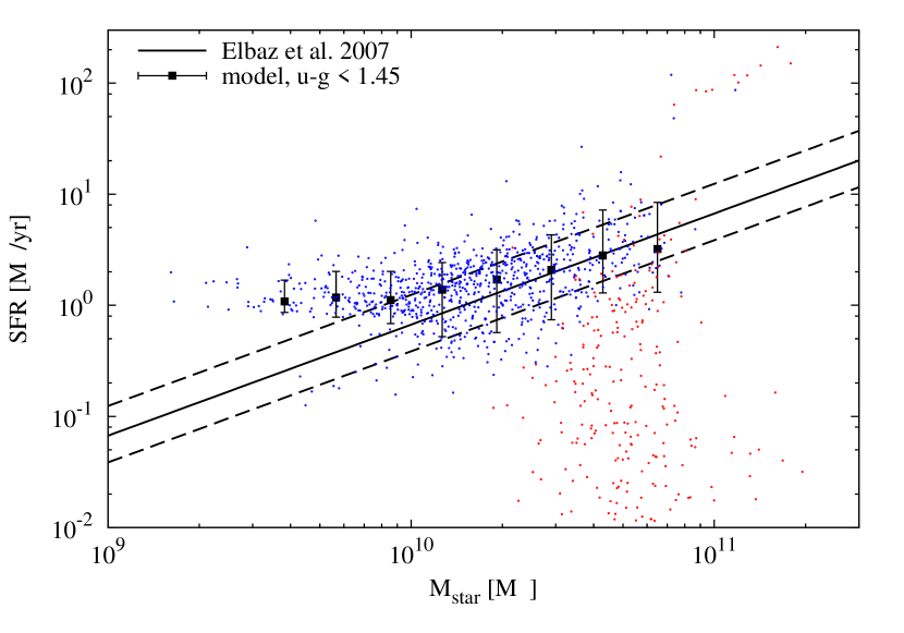
Figure 15: The stellar mass vs SFR relation for local galaxies. Both the SFR and stellar mass are converted into those with Salpeter IMF from those with Chabrier IMF, by multiplying by a factor of 1.8. The solid and dashed lines are the observed relation and typical error obtained by Elbaz et al. (2007). The blue and red dots show the distribution of star-forming and passive galaxies in the model, respectively. Here we adopt the same color criteria with Elbaz et al. (2007), i.e., the galaxies having blue color ($(u-g)<1.45$) are regarded as the star-forming while the others are regarded as passive. For the model, we only plot the galaxies brighter than $M_{B}=-20$ AB mag, which is the limiting magnitude of the sample of Elbaz et al. (2007). The black filled squares with error bars show the median and the 10th to the 90th percentile of star-forming galaxies in each bin of stellar mass.

5.7 Stellar-to-halo mass ratio

Figure 16 presents the ratio of the stellar mass of central galaxy to the total baryon mass in their host halo against the total mass of their host halo. The total baryon mass $M_{\rm bar}$ is simply estimated as $M_{\rm bar}=M_{\rm h}\times(\Omega_{\rm b}/\Omega_{\rm m})$. This plot indicates an efficiency of star formation as a function of halo mass, and can be a tight constraint on the galaxy formation model.

The median and the 10th to 90th percentiles of model galaxies in each halo mass bin are shown by the black squares with error bars. The solid and dashed lines show the average and $1\sigma$ confidence level estimated by Moster et al. (2013) using an “abundance matching technique”, in which the halo mass is estimated by matching the abundance of halos in N-body simulations to the abundance of observed galaxies. The prediction of our model well agree with the result of Moster et al. (2013). The distribution of stellar-to-halo mass ratio has a peak around $M_{\rm h}\sim 10^{12}M_{\odot}$. It reflects effects of SN feedback and AGN feedback: the former efficiently works in lower mass halos because the gravitational potential well is shallow in such halos, while the later efficiently works in massive halos because the cooling time is long enough and the central SMBH can sufficiently evolve in such halos.

Figure 16: The stellar mass of central galaxies relative to the total baryon mass in their host halo as a function of the total mass of host halo. The black filled squares with error bars denote the median and the 10th to 90th percentile of model galaxies in each bin of the host halo mass. The black solid and dashed lines show the average and $1\sigma$ confidence level of stellar mass ratio obtained by abundance matching technique (Moster et al. 2013). The total baryonic mass $M_{\rm bar}$ is estimated as $M_{\rm bar}=M_{\rm h}\times(\Omega_{\rm b}/\Omega_{\rm m})$.

5.8 Mass metallicity relation

Figure 17 shows the predicted relation between the stellar mass and the metallicity of cold gas for star forming galaxies. The median and the 16th to 84th percentile of the distribution of SDSS galaxies estimated by Tremonti et al. (2004) is also shown in figure 17 by solid lines. The cold gas metallicity is denoted by the gas-phase oxygen abundance in unit of $12+\log({\rm O/H})$. The solar metallicity in this unit is $8.93$ (Anders & Grevesse, 1989). The metallicity with respect to the solar metallicity, $Z_{\odot}=0.019$ (Anders & Grevesse 1989), is also indicated on the right-side axis of figure 17 for reference. We defined the “star-forming galaxy” as a galaxy with specific SFR (i.e., SFR/$M_{\rm star}$) higher than $10^{-11}{\rm yr}^{-1}$. If we change this threshold to more lower value, for example, the relation will shift towards high-metallicity.

Comparing with the observation, our model galaxies tend to have lower metallicities at the stellar mass range of $M_{\rm star}<10^{10}M_{\odot}$. We will investigate this issue in future paper.

Figure 17: Relation between stellar mass and cold gas metallicity, which is denoted by the gas-phase oxygen abundance in unit of $12+\log({\rm O/H})$. Solar metallicity in this unit is 8.93 (Anders & Grevesse 1989). The solid lines represents the 84th, 50th, and 16th percentile of local star-forming galaxies observed by SDSS (Tremonti et al. 2004). The black filled squares with error bars show the 84th, 50th, and 16th percentile of the distributions of model galaxies in each magnitude bin. For the model, we defined star forming galaxy as a galaxy which are larger than $10^{-11}$ yr^-1 in specific star formation rate (i.e., SFR/$M_{\rm star}$) .

6 Distant galaxies

In this section we show the model predictions for the basic properties of high-$z$ galaxies.

6.1 Cosmic star formation history

Figure 18 shows the redshift evolution of cosmic star formation rate density (i.e., total SFR of all galaxies per unit comoving volume). The blue solid line shows the result of our standard model ($\nu^{2}$GC-H2 model). The SFR of model galaxies are converted into those with Salpeter IMF from those Chabrier IMF, by multiplying a factor of 1.8. The $\nu^{2}$GC-H1 model is also shown by red solid line to see the effect of mass resolution. A discrepancy between these two models increases at high redshift, indicating that contributions from galaxies resides in lower mass halos become significant at high redshift.

The standard model well reproduces the observations. At a redshift greater than $z>4$, it seems that the model predictions are much greater than observed SFR density of Bouwens et al. (2014); however, their data only include galaxies brighter than $M(1500{\rm\AA})<-17.0$, while the other data and model predictions are integration in entire magnitude range. Furthermore, the survey of Bouwens et al. (2014) is designed to find galaxies having blue colors, and therefore they might miss a population of dusty red galaxies. In fact, the predicted UV luminosity density (i.e., total luminosity of all galaxies per unit comoving volume) is roughly consistent with the data of Bouwens et al. (2014) when the effect of limiting magnitude are taken into account (see next subsection).

Our model predicts that a large amount of star formation activity has not yet been observed at distant universe. It will be investigated by future observations.

6.2 Evolution of luminosity density in cosmic time

Figure 19 shows the predicted redshift evolution of the luminosity density at 1500 Å(thick solid line). The intrinsic luminosity density (i.e., without dust extinction) is shown by thick dotted line for reference. Note that the observational data plotted in figure 19 are not corrected for dust extinction effect thus they should be compared with the model with dust extinction (thick solid line). As already mentioned above, the data of Bouwens et al. (2014) only include galaxies brighter than $M(1500{\rm\AA})<-17.0$. The model prediction taking into account the same magnitude limit with the Bouwens et al. (2014) is shown by thin solid line. We can see that the model well reproduces the observations. This result support a validity of our modelings of star formation and dust extinction.

Figure 20 presents the redshift evolution of the sum of total IR luminosity ($8$–$1000$ ${\rm\mu m}$) of all galaxies per unit comoving volume. The total IR luminosity of model galaxies are estimated from the SED of each galaxy to be consistent with the total amount of stellar luminosity absorbed by dust. The observational data are obtained by Gruppioni et al. (2013), by integrating the total IR LFs down to $10^{8}L_{\odot}$. The model reproduces the observation within a factor of 2–3. The discrepancy between the model and observation is partly due to a contribution from AGNs, which is included in the observational data while not included in the model.

Figure 18: The cosmic SFR density as a function of redshift. The red and blue solid lines represent the predictions by model with the N-body data of $\nu^{2}$GC-H1 (red) and $\nu^{2}$GC-H2 (blue), respectively. The parameters related to baryon physics are the same in these models. We also show the observational data estimated by dust continuum (Pascale et al., 2009; Rodighiero et al., 2010; Karim et al., 2011) and UV continuum (Ouchi et al., 2004; Cucciati et al., 2012; Bouwens et al., 2014). The data of Hopkins (2004) are the compilation of various observations. All the data points are corrected for dust extinction, by the methods adopted in individual references. The data points of Bouwens et al. (2014) are obtained by integrating LF down to the $M_{\rm AB}$(1500 Å) $<$ -17.0, while the other observations and our model includes the contribution from all galaxies. The SFR of model galaxies are converted into those with Salpeter IMF from those Chabrier IMF, by multiplying a factor of 1.8.

Figure 19: The redshift evolution of luminosity density at 1500 Å. The filled circles and open triangles are observational data compiled by Hopkins (2004) and obtained by Bouwens et al. (2014), respectively. The model prediction is shown by solid black line. For the purpose of comparison, we also show the model without dust extinction (dotted line). Those model predictions include a contribution from all galaxies. The data points of Bouwens et al. (2014) are obtained by integrating LF down to the $M_{\rm AB}(1500\AA)<-17.0$ while the other observational data are integrated down to zero luminosity. The thin solid line show the model prediction taking into account the magnitude limit of $M_{\rm AB}(1500{\rm\AA})=-17.0$.

Figure 20: The model prediction for the redshift evolution of total IR luminosity density, comparing with the observational data Gruppioni et al. (2013). The total IR luminosity of model galaxies are calculated from the SED of each galaxy, to be consistent with the total amount of stellar luminosity absorbed by dust.

6.3 Redshift evolution of $K$-band luminosity function

Figure 21 shows the redshift evolution of rest-frame $K$-band LF. The observational data are obtained by Cirasuolo et al. (2010). The model well reproduces the bright-end of LFs even at $z=2.0$, which was not able to reproduce in our previous model. In new model, formation of massive galaxies are suppressed by AGN feedback only at low-redshift, and therefore the model can reproduce the bright-end LFs of local and high-$z$ galaxies at the same time. On the other hand, the model overestimates the abundance of dwarf galaxies over all redshift range. This discrepancy might suggest that SN feedback should be more efficient at high-$z$. However, there still remains some uncertainties in the observation. For example, cosmic variance, systematic error in $k$-correction, and incompleteness of the survey due to a surface brightness limit will affect the measurement of the faint-end slope of high-$z$ $K$-band LFs.

Figure 21: The redshift evolution of rest-frame $K$-band luminosity function. From top to bottom, we show the LFs at $z=0.5,1.0,1.5,2.0$. The solid black lines are model predictions. The black filled circles with error bars are the observational data obtained by Cirasuolo et al. (2010).

7 Summary

In this paper we present a new cosmological galaxy formation model, $\nu^{2}$GC, as an updated version of our previous model, $\nu$GC (Nagashima et al. 2005; see also Nagashima & Yoshii 2004). Major updates of the model are as follows: (1) the N-body simulations of the evolution of dark matter halos are updated (Ishiyama et al. 2015), (2) The formation and evolution process of SMBHs and the suppression of gas cooling due to the AGN activity (AGN feedback) is included, (3) heating of the intergalactic gas by the cosmic UV background is included, and (4) adopt a Markov chain Monte Carlo method in parameter tuning. Thanks to the updated N-body simulations, the minimum halo mass of the model reaches $1.37\times 10^{8}M_{\odot}$ in the best case, which is below the effective Jeans mass at high redshift. In our largest simulation box (1.12 Gpc/h), we can perform statistical analysis for rare objects such as bright quasars.

The main results of this paper are summarized as follows.

1. We tuned the model to fit the local $r$- and $K$-band LFs and HI MF by using a MCMC method. As a result, the model has succeeded well in reproducing these observables at the same time.

2. The model well reproduces the scaling relations between the size and the magnitude, and the rotation velocity and the magnitude of spiral galaxies. For elliptical galaxies, the model roughly well reproduces the observed size-magnitude relation and the velocity dispersion-magnitude relation. However, for bright elliptical galaxies, the model underpredicts both of the size and the velocity dispersion. We need to improve the model related to the galaxy merger and formation process of the bulge component.

3. The model well reproduces the observed bimodal distribution in color for bright galaxies. On the other hand, the model predicts redder color for dwarf galaxies comparing with the observations. This might be caused from our oversimplified prescription for star formation, SN feedback and stripping of hot gas.

4. For massive galaxies ($M_{\rm star}>10^{10}M_{\odot}$), model well reproduces the observed scaling relation between the stellar mass and gas phase metallicity at $z=0$. However the model underpredicts metallicity of dwarf galaxies. This might also be caused by our oversimplified treatment of star formation and SN feedback. In addition, assumed IMF would also affect it.

5. The observed scaling relation between the bulge mass and SMBH mass, and MF of local SMBHs are well reproduced in our model.

6. The cosmological evolution of star formation rate density and UV luminosity density predicted by our model are well agree with the observations. We found that the model roughly reproduces the redshift evolution of total IR luminosity density. We also compared the redshift evolution of the rest-frame $K$-band LFs, and found that the model well reproduces the bright-end of LFs at $0<z<2$.

Since the main aim of this paper is to present the details of the calculation method of our model, we compared the model only with some basic observables mentioned above. Subsequent papers will discuss another topics related to galaxy formation: the clustering properties of quasars, the origin of cosmic NIR background, the properties of sub-millimeter galaxies, for example.

The results of our model, including the LFs in several wavebands, mass functions, and the mock galaxies, are publicly available on the web.

We would like to thank for the anonymous referee for many useful comments. This study has been funded by Yamada Science Foundation, MEXT HPCI STRATEGIC PROGRAM. The $\nu^{2}$GC simulations were partially carried out on the Aterui supercomputer at theCenter for Computational Astrophysics (CfCA) of the National Astronomical Observatory of Japan, and the K computer at the RIKEN Advanced Institute for Computational Science (Proposal numbers hp120286, hp130026, and hp140212). RM has been supported by the Grant-in-Aid for JSPS Fellows. MN has been supported by the Grant-in-Aid for the Scientific Research Fund (25287041) commissioned by the Ministry of Education, Culture, Sports, Science and Technology (MEXT) of Japan. TO acknowledges the financial support of Japan Society for the Promotion of Science (JSPS) Grant-in-Aid for Young Scientists (B: 224740112). TI has been supported by MEXT/JSPS KAKENHI Grant Number 15K12031.

References

- Anders & Grevesse (1989) Anders E., Grevesse N., 1989, GeCoA, 53, 197
- Avila et al. (2014) Avila S., Knebe A., Pearce F. R., et al., 2014, MNRAS, 441, 3488
- Baldry et al. (2004) Baldry I. K., Glazebrook K., Brinkmann J., Ivezić Ž., Lupton R. H., Nichol R. C., Szalay A. S., 2004, ApJ, 600, 681
- Baldry et al. (2012) Baldry, I. K., Driver, S. P., Loveday, J., et al. 2012, MNRAS, 421, 621
- Baugh et al. (1996) Baugh C. M., Cole S., Frenk C. S., 1996, MNRAS, 283, 1361
- Barnes & Hernquist (1996) Barnes, J. E., & Hernquist, L. 1996, ApJ, 471, 115
- Bender et al. (1992) Bender R., Burstein D., Faber S. M., 1992, ApJ, 399, 462
- Bender & Nieto (1990) Bender R., Nieto J.-L., 1990, A&A, 239, 97
- Benson (2014) Benson A. J., 2014, MNRAS, 444, 2599
- Bett et al. (2007) Bett P., Eke V., Frenk C. S., Jenkins A., Helly J., Navarro J., 2007, MNRAS, 376, 215
- Binney & Tremaine (1987) Binney, J., & Tremaine, S. 1987, Galactic Dynamics, Princeton Univ. Press, Princeton, NJ
- Blanton et al. (2005) Blanton M. R., Lupton R. H., Schlegel D. J., Strauss M. A., Brinkmann J., Fukugita M., Loveday J., 2005, ApJ, 631, 208
- Boylan-Kolchin et al. (2009) Boylan-Kolchin M., Springel V., White S. D. M., Jenkins A., Lemson G., 2009, MNRAS, 398, 1150
- Bower et al. (2006) Bower R. G., Benson A. J., Malbon R., Helly J. C., Frenk C. S., Baugh C. M., Cole S., Lacey C. G., 2006, MNRAS, 370, 645
- Bouwens et al. (2014) Bouwens R. J., Illingworth G. D., Oesch P. A., et al., 2014, ApJ, 793, 115
- Brinchmann et al. (2004) Brinchmann J., Charlot S., White S. D. M., Tremonti C., Kauffmann G., Heckman T., Brinkmann J., 2004, MNRAS, 351, 1151
- Bullock et al. (2001a) Bullock, J.S., Kolatt, T.S., Sigad, T., Somerville, R.S., Kravtsov, A.V., Klypin, A.A., Primack, J.R., & Dekel, A. 2001, MNRAS, 321, 559
- Bullock et al. (2001b) Bullock J. S., Dekel A., Kolatt T. S., Kravtsov A. V., Klypin A. A., Porciani C., Primack J. R., 2001, ApJ, 555, 240
- Burstein et al. (1997) Burstein D., Bender R., Faber S., Nolthenius R., 1997, AJ, 114, 1365
- Bruzual & Charlot (2003) Bruzual G., Charlot S., 2003, MNRAS, 344, 1000
- Calzetti et al. (2000) Calzetti D., Armus L., Bohlin R. C., Kinney A. L., Koornneef J., Storchi-Bergmann T., 2000, ApJ, 533, 682
- Chabrier (2003) Chabrier G., 2003, PASP, 115, 763
- Cirasuolo et al. (2010) Cirasuolo, M., McLure, R. J., Dunlop, J. S., et al. 2010, MNRAS, 401, 1166 , 11
- Cole et al. (1994) Cole S., Aragon-Salamanca A., Frenk C. S., Navarro J. F., Zepf S. E., 1994, MNRAS, 271, 781
- Cole et al. (2000) Cole S., Lacey C. G., Baugh C. M., Frenk C. S., 2000, MNRAS, 319, 168
- Colpi (2014) Colpi M., 2014, SSRv, 183, 189
- Couchman & Rees (1986) Couchman, H. M. P., & Rees, M. J. 1986, MNRAS, 221, 53
- Courteau et al. (2000) Courteau S., Willick J. A., Strauss M. A., Schlegel D., Postman M., 2000, ApJ, 544, 636
- Courteau et al. (2007) Courteau S., Dutton A. A., van den Bosch F. C., MacArthur L. A., Dekel A., McIntosh D. H., Dale D. A., 2007, ApJ, 671, 203
- Croton et al. (2006) Croton, D. J., Springel, V., White, S. D. M., et al. 2006, MNRAS, 365, 11
- Cucciati et al. (2012) Cucciati, O. et al. 2012, A&A, 539, A31
- Daddi et al. (2007) Daddi E., Dickinson M., Morrison G., et al., 2007, ApJ, 670, 156
- Dale et al. (1999) Dale D. A., Giovanelli R., Haynes M. P., Campusano L. E., Hardy E., 1999, AJ, 118, 1489
- Davis et al. (1985) Davis M., Efstathiou G., Frenk C. S., White S. D. M., 1985, ApJ, 292, 371
- Davis & Laor (2011) Davis S. W., Laor A., 2011, ApJ, 728, 98
- Dekel & Silk (1986) Dekel A., Silk J., 1986, ApJ, 303, 39
- De Lucia et al. (2010) De Lucia G., Boylan-Kolchin M., Benson A. J., Fontanot F., Monaco P., 2010, MNRAS, 406, 1533
- Di Matteo et al. (2005) Di Matteo, T., Springel, V. & Hernquist, L. 2005, Nature, 7026, 604
- Disney et al. (1989) Disney, M., Davies, J., & Phillipps, S. 1989, MNRAS, 239, 939
- Doroshkevich et al. (1967) Doroshkevich, A. G., Zel’dovich, Y. B., & Novikov, I. D. 1967, Soviet Ast., 11, 233
- Driver et al. (2012) Driver, S. P., Robotham, A. S. G., Kelvin, L., et al. 2012, MNRAS, 427, 3244
- Elahi et al. (2013) Elahi P. J., Han J., Lux H., et al., 2013, MNRAS, 433, 1537
- Elbaz et al. (2007) Elbaz D., Daddi E., Le Borgne D. et al., 2007, A&A, 468, 33
- Enoki et al. (2003) Enoki M., Nagashima M., Gouda N., 2003, PASJ, 55, 133
- Enoki et al. (2004) Enoki M., Inoue K. T., Nagashima M., Sugiyama N., 2004, ApJ, 615, 19
- Enoki & Nagashima (2007) Enoki M., Nagashima M., 2007, PThPh, 117, 241
- Enoki et al. (2014) Enoki M., Ishiyama T., Kobayashi M. A. R., Nagashima M., 2014, ApJ, 794, 69
- Faber & Jackson (1976) Faber S. M., Jackson R. E., 1976, ApJ, 204, 668
- Faber et al. (1989) Faber S. M., Wegner G., Burstein D., Davies R. L., Dressler A., Lynden-Bell D., Terlevich R. J., 1989, ApJS, 69, 763
- Fall (1979) Fall, S. M. 1979, Nature, 281, 200
- Fall & Efstathiou (1980) Fall, S. M., & Efstathiou, G. 1980, MNRAS, 193, 189
- Fall (1983) Fall, S. M. 1983, in ‘Internal kinematics and dynamics of galaxies’, proceedings of the IAU symposium 100, Besancon, France, Dordrecht, D. Reidel, p.391
- Firth et al. (2007) Firth P., Drinkwater M. J., Evstigneeva E. A., Gregg M. D., Karick A. M., Jones J. B., Phillipps S., 2007, MNRAS, 382, 1342
- Forbes et al. (2008) Forbes D. A., Lasky P., Graham A. W., Spitler L., 2008, MNRAS, 389, 1924
- Gelman & Rubin (1992) Gelman A., Rubin D., 1992, Stat. Sci., 7, 457
- Gnedin (2000) Gnedin, N. Y. 2000, ApJ, 542, 535
- Gruppioni et al. (2013) Gruppioni C., Pozzi F., Rodighiero G., et al., 2013, MNRAS, 432, 23
- Gonzalez-Perez et al. (2014) Gonzalez-Perez V., Lacey C. G., Baugh C. M., Lagos C. D. P., Helly J., Campbell D. J. R., Mitchell P. D., 2014, MNRAS, 439, 264
- Hastings (1970) Hastings, W. K., 1970, Biometrika, 57, 97
- Haynes et al. (2011) Haynes M. P., Giovanelli R., Martin A. M., et al., 2011, AJ, 142, 170
- Henriques et al. (2009) Henriques B. M. B., Thomas P. A., Oliver S., Roseboom I., 2009, MNRAS, 396, 535
- Hopkins (2004) Hopkins A. M., 2004, ApJ, 615, 209
- Hopkins et al. (2005) Hopkins, P. F., Hernquist, L., Cox, T. J., et al. 2005, ApJ, 630, 705
- Hopkins et al. (2006) Hopkins, P. F., Hernquist, L., Cox, T. J., et al. 2006, ApJS, 163, 1
- Hopkins et al. (2009) Hopkins P. F., Hernquist L., Cox T. J., Keres D., Wuyts S., 2009, ApJ, 691, 1424
- Ishiyama et al. (2009) Ishiyama T., Fukushige T., Makino J., 2009, PASJ, 61, 1319
- Ishiyama et al. (2012) Ishiyama, T., Nitadori, K., Makino, J. 2012, in Proc. Int. Conf. High Performance Computing, Networking, Storage and Analysis, SC’12 (Los Alamitos, CA: IEEE Computer Society Press), 5:, (arXiv:1211.4406)
- Ishiyama et al. (2015) Ishiyama T., Enoki M., Kobayashi M. A. R., Makiya R., Nagashima M., Oogi T., 2015, PASJ, 67, 61
- Jaffe (1983) Jaffe, W. 1983, MNRAS, 202, 995
- Jiang et al. (2008) Jiang C. Y., Jing Y. P., Faltenbacher A., Lin W. P., Li C., 2008, ApJ, 675, 1095
- Jiang et al. (2010) Jiang C. Y., Jing Y. P., Lin W. P., 2010, A&A, 510, A60
- Karim et al. (2011) Karim, A. et al. 2011, ApJ, 730, 61
- Kauffmann & White (1993) Kauffmann G., White S. D. M., 1993, MNRAS, 261, 921
- Kauffmann et al. (1993b) Kauffmann G., White S. D. M., Guiderdoni B., 1993, MNRAS, 264, 201
- Keres et al. (2003) Keres D., Yun M. S., Young J. S., 2003, ApJ, 582, 659
- Knebe et al. (2011) Knebe A., Knollmann S. R., Muldrew S. I., et al., 2011, MNRAS, 415, 2293
- Knebe et al. (2015) Knebe A., Pearce F. R., Thomas P. A., et al., 2015, MNRAS, 451, 4029
- Kobayashi et al. (2007) Kobayashi M. A. R., Totani T., Nagashima M., 2007, ApJ, 670, 919
- Kobayashi et al. (2010) Kobayashi M. A. R., Totani T., Nagashima M., 2010, ApJ, 708, 1119
- Koyama et al. (2008) Koyama H., Nagashima M., Kakehata T., Yoshii Y., 2008, MNRAS, 389, 237
- Kuzmin (1952) Kuzmin G., 1952, Publ. Astron. Obs. Tartu, 32, 311
- Kuzmin (1956) Kuzmin G., 1956, Astron. Zh., 33, 27
- Lacey & Cole (1993) Lacey, C.G., & Cole, S. 1993, MNRAS, 262, 627
- Lagos et al. (2014) Lagos C. d. P., Davis T. A., Lacey C. G., Zwaan M. A., Baugh C. M., Gonzalez-Perez V., Padilla N. D., 2014, MNRAS, 443, 1002
- Lee et al. (2014) Lee J., Yi S. K., Elahi P. J., et al., 2014, MNRAS, 445, 4197
- Lu et al. (2012) Lu, Y., Mo, H. J., Katz, N., & Weinberg, M. D. 2012, MNRAS, 421, 1779
- Lu et al. (2014) Lu, Y., Mo, H. J., Lu, Z., Katz, N., & Weinberg, M. D. 2014, MNRAS, 443, 1252
- Macciò et al. (2008) Macciò A. V., Dutton A. A., van den Bosch F. C., 2008, MNRAS, 391, 1940
- Madau & Dickinson (2014) Madau P., Dickinson M., 2014, ARA&A, 52, 415
- Maeder (1992) Maeder, A. 1992, A&A, 264, 105
- Makino & Hut (1997) Makino, J., & Hut, P. 1997, ApJ, 481, 83
- Makiya et al. (2011) Makiya R., Totani T., Kobayashi M. A. R., 2011, ApJ, 728, 158
- Makiya et al. (2014) Makiya R., Totani T., Kobayashi M. A. R., Nagashima M., & Takeuchi T. T., 2014, MNRAS, 441, 63
- Martin et al. (2010) Martin A. M., Papastergis E., Giovanelli R., Haynes M. P., Springob C. M., Stierwalt S., 2010, ApJ, 723, 1359
- Mathewson et al. (1992) Mathewson D. S., Ford V. L., Buchhorn M., 1992, ApJS, 81, 413
- Matković & Guzmán (2005) Matković A., Guzmán R., 2005, MNRAS, 362, 289
- McConnell & Ma (2013) McConnell, N. J. & Ma, C.-P., 2013, ApJ, 764, 181
- Metropolis et al. (1953) Metropolis, N., Rosenbluth, A. W., Rosenbluth, M. N., Teller, A. H., & Teller, E. 1953, J. Chem. Phys., 21, 1087
- Mihos & Hernquist (1994) Mihos, J. C., & Hernquist, L. 1994, ApJ, 431, L9
- Mihos & Hernquist (1996) Mihos, J. C., & Hernquist, L. 1996, ApJ, 464, 641
- Mo et al. (1998) Mo, H.J., Mao, S., & White, S.D.M. 1998, MNRAS, 295, 319
- Monaco et al. (2007) Monaco P., Fontanot F., Taffoni G., 2007, MNRAS, 375, 1189
- Monaco et al. (2014) Monaco P., Benson A. J., De Lucia G., Fontanot F., Borgani S., Boylan-Kolchin M., 2014, MNRAS, 441, 2058
- Moore et al. (2002) Moore S. A. W., Lucey J. R., Kuntschner H., Colless M., 2002, MNRAS, 336, 382
- Moster et al. (2013) Moster B. P., Naab T., White S. D. M., 2013, MNRAS, 428, 3121
- Nagashima & Yoshii (2003) Nagashima, M., & Yoshii, Y. 2003, MNRAS, 340, 509
- Nagashima & Yoshii (2004) Nagashima M., Yoshii Y., 2004, ApJ, 610, 23
- Nagashima et al. (2005) Nagashima M., Yahagi H., Enoki M., Yoshii Y., Gouda N., 2005, ApJ, 634, 26 (N05)
- Navarro, Frenk & White (1997) Navarro J. F., Frenk C. S., White S. D. M., 1997, MNRAS, 490, 493
- Okamoto & Habe (1999) Okamoto, T., & Habe, A. 1999, ApJ, 516, 591
- Okamoto & Habe (2000) Okamoto, T., & Habe, A. 2000, PASJ, 52, 457
- Okamoto et al. (2008) Okamoto, T., Gao, L., & Theuns, T. 2008, MNRAS, 390, 920
- Okoshi & Nagashima (2005) Okoshi K., Nagashima M., 2005, ApJ, 623, 99
- Okoshi et al. (2010) Okoshi K., Nagashima M., Gouda N., Minowa Y., 2010, ApJ, 710, 1295
- Onions et al. (2012) Onions J., Knebe A., Pearce F. R., et al., 2012, MNRAS, 423, 1200
- Oogi et al. (2016) Oogi T., Enoki M., Ishiyama T., Kobayashi M. A. R., Makiya R., Nagashima M., 2016, MNRAS, 456, L30
- Ouchi et al. (2004) Ouchi, M. et al. 2004, ApJ, 611, 685
- Pascale et al. (2009) Pascale, E. et al. 2009, ApJ, 707, 1740
- Planck Collaboration et al. (2014) Planck Collaboration, Ade P. A. R., Aghanim N., et al., 2014, A&A, 571, A16
- Power et al. (2010) Power, C., Baugh, C. M., & Lacey, C. G. 2010, MNRAS, 406, 43
- Prada et al. (2012) Prada F., Klypin A. A., Cuesta A. J., Betancort-Rijo J. E., Primack J., 2012, MNRAS, 423, 3018
- Rodighiero et al. (2010) Rodighiero, G. et al. 2010, A&A, 515, A8
- Roukema et al. (1997) Roukema B. F., Quinn P. J., Peterson B. A., Rocca-Volmerange B., 1997, MNRAS, 292, 835
- Salim et al. (2007) Salim S., Rich R. M., Charlot S., et al., 2007, ApJS, 173, 267
- Sánchez-Conde & Prada (2014) Sánchez-Conde M. A., Prada F., 2014, MNRAS, 442, 2271
- Shankar et al. (2004) Shankar F., Salucci P., Granato G. L., De Zotti G., Danese L., 2004, MNRAS, 354, 1020
- Shankar et al. (2013) Shankar F., Marulli F., Bernardi M., Mei S., Meert A., Vikram V., 2013, MNRAS, 428, 109
- Shimizu et al. (2002) Shimizu, M., Kitayama, T., Sasaki, S., & Suto, Y. 2002, PASJ, 54, 645
- Shirakata et al. (2015) Shirakata H., Okamoto T., Enoki M., Nagashima M., Kobayashi M. A. R., Ishiyama T., Makiya R., 2015, MNRAS, 450, L6
- Simien & de Vaucouleurs (1986) Simien F., de Vaucouleurs G., 1986, ApJ, 302, 564
- Springel et al. (2005) Springel V., White S. D. M., Jenkins A., et al., 2005, Natur, 435, 629
- Springel (2012) Springel V., 2012, AN, 333, 515
- Somerville & Primack (1999) Somerville R. S., Primack J. R., 1999, MNRAS, 310, 1087
- Somerville (2002) Somerville R. S., 2002, ApJ, 572, L23
- Somerville & Davé (2014) Somerville R. S., Davé R. 2014, arXiv, arXiv:1412.2712
- Srisawat et al. (2013) Srisawat C., Knebe A., Pearce F. R., et al., 2013, MNRAS, 436, 150
- Sutherland & Dopita (1993) Sutherland, R., & Dopita, M. A. 1993, ApJS, 88, 253
- Trager et al. (2000) Trager S. C., Faber S. M., Worthey G., González J. J., 2000, AJ, 120, 165
- Tremonti et al. (2004) Tremonti C. A., Heckman T. M., Kauffmann G., et al., 2004, ApJ, 613, 898
- Tully & Fisher (1977) Tully R. B., Fisher J. R., 1977, A&A, 54, 661
- Tully et al. (1996) Tully R. B., Verheijen M. A. W., Pierce M. J., Huang J.-S., Wainscoat R. J., 1996, AJ, 112, 2471
- Verheijen (2001) Verheijen M. A. W., 2001, ApJ, 563, 694
- Wetzel (2011) Wetzel, A. R. 2011, MNRAS, 412, 49
- White & Frenk (1991) White S. D. M., Frenk C. S., 1991, ApJ, 379, 52
- Yoshii & Arimoto (1987) Yoshii Y., Arimoto N., 1987, A&A, 188, 13
- Zwaan et al. (2005) Zwaan M. A., Meyer M. J., Staveley-Smith L., Webster R. L., 2005, MNRAS, 359, L30