The effect of vertex corrections on the possibility of chiral symmetry breaking, induced by long-range Coulomb repulsion in graphene

Abstract

In  this paper we consider the possibility of chiral (charge or spin density wave) symmetry breaking in graphene due to long-range Coulomb interaction by comparing the results of the Bethe-Salpeter and functional renormalization-group approaches. The former approach performs summation of ladder diagrams in the particle-hole channel, and reproduces the results of the Schwinger-Dyson approach for the critical interaction strength of the quantum phase transition. The renormalization-group approach combines the effect of different channels and allows to study the role of vertex corrections. The critical interaction strength, which is necessary to induce the symmetry breaking in the latter approach is found in the static approximation to be $\alpha_{c}=e^{2}/(\epsilon v_{F})\approx 1.05$ without considering the Fermi velocity renormalization, and $\alpha_{c}=3.7$ with accounting the renormailzation of the Fermi velocity. The latter value is expected to be however reduced, when the dynamic screening effects are taken into account, yielding the critical interaction, which is comparable to the one in freely suspended graphene. We show that the vertex corrections are crucially important to obtain the mentioned values of critical interactions.

I Introduction

The fascinating physics of Dirac fermions, interacting via static Coulomb potential, became a subject of intensive research in condensed-matter physics after the experimental realization of graphene Novoselov . Despite vanishing density of states at the Fermi level in clean graphene, Coulomb interaction may lead to different instabilities of electronic system Herbut ; Honerkamp ; Rev ; Herbut1 . Even before the experimental discovery of graphene, the possibility of excitonic instability (related to the charge density wave formation) in this material was predicted theoreticallyKhveschenko ; Gusynin0 . It was argued, that sufficiently strong Coulomb interaction is able to open a gap in the excitation spectrum analogously to the chiral symmetry breaking in quantum electrodynamicsCSB .

The analysis within the Schwinger-Dyson mean-field approach Khveschenko1 ; Murthy ; Gusynin in the static approximation found critical Coulomb interaction, which is necessary to open the charge gap, to be $\alpha_{c}=e^{2}/(\epsilon v_{F})=1.62$ (see, e.g., discussion in Ref. Gusynin, ), where $e$ is the critical charge, $\epsilon$ corresponds to substrate dielectric constant, and $v_{F}$ is the Fermi velocity. This result is not very far from the result of quantum Monte-Carlo approach MC $\alpha_{c}=1.08$. Inclusion of the dynamic screening of Coulomb interaction in Refs. Khveschenko-vel-dyn, ; Gusynin1, allowed to improve further the agreement with the numerical results. These results were however altered recently by considering the effect of renormalization of Fermi velocity, yielding critical Coulomb interactions, which depend on the approximation used, namely the critical couplings $\alpha_{c}=1.75$ (Ref. Gonzalez, ), $\alpha_{c}=7.65$ (Ref. Popovici, ), and $\alpha_{c}=3.1$ (Ref. Gonzalez1, ) were obtained. The latter result seems to be most reliable within the Schwinger-Dyson approach, since it accounts for the renormalization of quasiparticle weight and the polarization bubble. These later results are all larger than the coupling constant of free-suspended graphene, in agreement with the experimental fact, that freely suspended graphene shows no chiral instabilityExp . On the other hand, the important effect of the other bands for increasing critical Coulomb interaction was emphasized in Ref. Katsnelson .

In the present paper we concentrate on studying the effect of the long-range part of Coulomb interaction and address the question, in which parameter range the Schwinger-Dyson approach is applicable. Indeed, this approach, which can be reformulated as a ladder approximation for electron interaction vertices, neglects contribution of the channels, other than the particle-hole one. From previous studies of the two-dimensional Hubbard model with short-range (on-site) interactionHonerkampRice ; Metzner ; Katanin ; 1PIRev ; Honerkamp , it is known that the contribution of the particle-hole channel is to a large extent compensated by the particle-particle channel. For the systems with Dirac electronic dispersion this cancellation is almost perfect, since the electronic Green function is odd with respect to momentum and frequency. At a first glance, this can strongly weaken the possibility of excitonic instability in graphene.

Apart from that, the discussed approaches neglect electron-electric field vertex corrections, which also appear beyond the ladder approximation, used in these studies. Although these corrections are expected to have no infrared divergencies Kotov ; Sodemann , in the lowest (second) order in the Coulomb interaction they increase renormalized dielectric constant of the substrate. Therefore, one could expect that they yield further increase of the critical value of the Coulomb interaction for the chiral quantum phase transition.

The possibility of chiral phase transition in graphene was considered previously within the field-theoretical renormalization group approachSon ; Son1 ; FostAleiner ; Herbut2 ; Sarma . It was shown that in the one-loop approximation Son ; Son1 ; FostAleiner ; Herbut2 Coulomb interaction is irrelevant due to increase of the Fermi velocity with respect to its bare value. Apart from that, small point-like interactions, which can be added to test the (in)stability towards chiral symmetry breaking, are also irrelevant because of the abovementioned cancellation between particle-particle and particle-hole channels. Therefore, this approach does not yield divergence of some coupling constants at sufficiently large Coulomb interaction, and therefore does not yield chiral phase transition. In the two-loop approximation Sarma there is an instability of the field-theoretical RG flow at $\alpha_{c}=0.78,$ which can be in principle related to a possibility of chiral phase transition. However, such a scenario is anyhow different from the two-particle instability considered within the Schwinger-Dyson approach.

In the study paper we apply the functional renormalization-group (fRG) approachHonerkampRice ; Metzner ; Katanin ; 1PIRev ; Honerkamp and argue that considering momentum dependences of the vertices and summing all contributions from different channels in the one-loop approximation, the so far neglected effect of the vertex corrections yields at the same time enhancing the tendency towards excitonic instability, and to a large extent compensates the above mentioned factors, which weaken the instability. Taken together, they yield even smaller result for the critical interaction strength, than in the ladder approach. In the static approximation without the renormalization of Fermi velocity we obtain $\alpha_{c}=1.05,$ which is smaller than previous estimates at the same level of approximation within the Schwinger-Dyson approach. The critical interaction increases to $\alpha_{c}^{v}=3.7$ when the Fermi velocity renormalization is taken into account. The latter value of the critical interaction is however expected to be reduced when the dynamic effects are taken into account, yielding the critical coupling, which is comparable to the one in the freely suspended graphene.

The outline of the paper is the following. In Section II we formulate the model, in Sect. III we discuss reformulation of Dyson-Schwinger approach as summation of ladder diagrams and extend previously obtained results to the symmetric phase. In Sect. IV we consider functional renormalization-group approach, discuss parametrization of the vertices used in the present study, and present main results for the electron interaction vertices. The Conclusion is presented in Sect. V.

II The model

To study electron interaction in graphene we consider the model (see, e.g., Refs. Son ; Son1 ; FostAleiner )

$$L_{0} = -\int d^{3}X\overline{\psi}_{s}(\gamma_{\mu}\partial_{\mu}+i\gamma_{0}A_{0})\psi_{s}$$ (1)

$$+\frac{1}{4\pi e^{2}}\int d^{3}Xdz\left[(\partial_{a}A_{0})^{2}+(\partial_{z}A_{0})^{2}\right]$$

where $\psi_{s}\equiv\psi_{s}(X)$ is the 4-spinor describing electronic degrees of freedom, $s=\uparrow,\downarrow$ is the spin projection, $X=(\tau,x,y),$ $\mu=0,1,2,$ $a=1,2,$ $\partial=(\partial_{\tau},v_{F}\partial_{x},v_{F}\partial_{y}),$ $\overline{\psi}=\psi^{+}\gamma_{0},\ \gamma_{\mu}$ are the Dirac matrices, e.g.

$$\gamma_{0}=\left(\begin{array}[]{cc}\sigma_{3}&0\\ 0&-\sigma_{3}\end{array}\right),\ \ \gamma_{a}=\left(\begin{array}[]{cc}\sigma_{a}&0\\ 0&-\sigma_{a}\end{array}\right),$$ (2)

where $\sigma_{i}$ are the Pauli matrices, $\alpha=e^{2}/(\epsilon v_{F})$ is the dimensionless coupling constant. The quadratic part of the action (1) represents the continuum limit of the microscopic tight-binding model of graphene (see, e.g., Ref. FostAleiner ) and corresponds to the representation $\psi=\{\psi_{A}^{1},\psi_{B}^{1},\psi_{B}^{2},-\psi_{A}^{2}\}$ ($\psi_{s}^{m}$ is an annihilation operator for the electron in valley $m$ and sublattice $s$). The scalar field $A_{0}$ accounts for the Coulomb interaction of Dirac particles, which is integrated along the third coordinate $z$, transverse to the graphene layer. Excluding $z$ direction, perpendicular to the graphene layer, and performing Fourier transformation, yields the effective actionSon ; Son1 ; FostAleiner

$$L_{0} = -\int\frac{d^{3}pd^{3}q}{(2\pi)^{6}}\overline{\psi}_{ps}\left[i\gamma_{\mu}p_{\mu}\delta(q)+i\gamma_{0}A_{0q}\right]\psi_{p+q,s}$$ (3)

$$+\frac{1}{4\pi\alpha}\int\frac{d^{3}q}{(2\pi)^{3}}|\mathbf{q}|A_{0q}A_{0,-q}$$

where $p_{\mu}=(\nu/v_{F},p_{x},p_{y})$ is the $3$-vector, including Matsubara frequency $\nu$ (and similar for $q$). It is well known (see, e.g., Ref. Rev ), that due to vanishing density of states, the Coulomb interaction in graphene is not screened, since the particle-hole bubble

$$\Pi(\mathbf{q},\omega)=\frac{q^{2}}{4\sqrt{q^{2}+(\omega/v_{F})^{2}}}$$ (4)

(where $q=|\mathbf{q}|$) is itself linear in momentum at $\omega=0.$ Therefore, summation of the bubble contributions in a rundom phase approximation (RPA) yields renormalization of the dielectric constant only, such that the effective ”screened” Coulomb interaction is

$$\alpha_{r}=\alpha/(1+\pi\alpha/2).$$ (5)

III The ladder (Bethe-Salpeter) approach without Fermi velocity renormalization

The Coulomb interaction may lead to excitonic (charge or spin density wave) instability with opening the gap in the electronic spectrum Khveschenko ; Gusynin0 ; Khveschenko1 ; Murthy ; Gusynin . The simplest way to treat this possibility is the Bethe-Salpeter approach. Here we consider the instability from the symmetric phase, which complements previous studies of symmetry-broken phase within the Schwinger-Dyson approachKhveschenko ; Gusynin0 ; Khveschenko1 ; Murthy ; Gusynin . The (linearized) gap equation of the Schwinger-Dyson approach in the static approximation (5) has the form

$$\Delta_{\mathbf{p}}=\Delta_{0}+2\pi\alpha_{r}\int\limits_{0}^{\Lambda}\frac{d^{2}\mathbf{k}}{(2\pi)^{2}}\mathrm{Tr}\left[\frac{\gamma_{0}\otimes\gamma_{0}}{|\mathbf{p}-\mathbf{k}|}\widetilde{\Pi}_{\mathrm{ph}}(\mathbf{k},\mathbf{0})\right]\Delta_{\mathbf{k}},$$ (6)

where we have introduced the bubble

$$\widetilde{\Pi}_{\mathrm{ph,pp}}(\mathbf{k},\mathbf{q}) = -\int\frac{d\varepsilon}{2\pi}\left[G(\mathbf{k},i\varepsilon)\otimes G(\pm\mathbf{k+q},\pm i\varepsilon)\right]$$ (7)

$$= \pm\frac{v_{F}}{2(v_{F}(|\mathbf{k}|)|\mathbf{k}|+v_{F}(|\mathbf{k\pm q}|)|\mathbf{k\pm q}|)}$$

$$\times \left[\gamma_{0}\otimes\gamma_{0}+\frac{k_{a}(k_{b}\pm q_{b})}{|\mathbf{k}||\mathbf{k\pm q}|}\gamma_{a}\otimes\gamma_{b}\right]$$

(the bubble $\widetilde{\Pi}_{\mathrm{pp}}$ will be used later, in Sect. IV), $G(\mathbf{k},\varepsilon)=\left(\gamma_{0}\varepsilon+\mathrm{i}v_{F}(|\mathbf{k|})\gamma_{a}k_{a}\right)^{-1}$, the matrices in the direct product act in the space of spinor indices of each fermionic line, $\Delta_{0}$ is the bare value of the gap, and in general the renormalized Fermi velocity $v_{F}(|\mathbf{k}|)$ depends on momentum. In the present Section we neglect the renormalization of the Fermi velocity by taking $v_{F}(|\mathbf{k|})=v_{F}$. The Eq. (6) can be iterated to express the resulting gap

$$\Delta_{\mathbf{p}}=\Delta_{0}\left\{1+\int\limits_{0}^{\Lambda}\frac{d^{2}\mathbf{k}}{(2\pi)^{2}}\mathrm{Tr}\left[\Gamma_{\mathbf{pk0}}\widetilde{\Pi}_{\mathrm{ph}}(\mathbf{k},\mathbf{0})\right]\right\}$$ (8)

through the vertex function $\Gamma_{\mathbf{kk}^{\prime}\mathbf{q}},$ for which we obtain the integral equation

$$\Gamma_{\mathbf{kk}^{\prime}\mathbf{q}} = \frac{2\pi\alpha_{r}}{|\mathbf{k}-\mathbf{k}^{\prime}|}\gamma_{0}\otimes\gamma_{0}$$

$$+ \gamma_{0}\otimes\gamma_{0}\int\frac{d^{2}p}{(2\pi)^{2}}\frac{2\pi\alpha_{r}}{|\mathbf{k}-\mathbf{p}|}\widetilde{\Pi}_{\mathrm{ph}}(\mathbf{p},\mathbf{q})\Gamma_{\mathbf{pk}^{\prime}\mathbf{q}},$$

corresponding to the summation of ladder diagrams in the particle-hole channel. At $\mathbf{q}=0$ we therefore have

$$\Gamma_{\mathbf{kk}^{\prime}\mathbf{0}} = \frac{2\pi\alpha_{r}}{|\mathbf{k}-\mathbf{k}^{\prime}|}\gamma_{0}\otimes\gamma_{0}+\frac{\alpha_{r}}{4}\int dp\int\frac{d\theta_{p}}{2\pi}\frac{1}{|\mathbf{k}-\mathbf{p}|}$$ (10)

$$\times \left(I\otimes I+\frac{p_{a}p_{b}}{|\mathbf{p}|^{2}}\gamma_{0}\gamma_{a}\otimes\gamma_{0}\gamma_{b}\right)\Gamma_{\mathbf{pk}^{\prime}\mathbf{0}}.$$

We search the solution to this equation in the form

$$\Gamma_{\mathbf{kk}^{\prime}\mathbf{0}} = \Gamma_{\mathbf{kk}^{\prime}\mathbf{0}}^{0}\gamma_{0}\otimes\gamma_{0}+\Gamma_{\mathbf{kk}^{\prime}\mathbf{0}}^{1}\gamma_{a}\otimes\gamma_{a}$$ (11)

$$+ \Gamma_{\mathbf{kk}^{\prime}\mathbf{0}}^{12}i\gamma_{0}\gamma_{1}\gamma_{2}\otimes i\gamma_{0}\gamma_{1}\gamma_{2}.$$

Performing matrix multiplication (see Appendix A), for the s-component of the vertices $\Gamma_{\mathbf{kk}^{\prime}\mathbf{0}}^{m},$ which are obtained by averaging over direction of vecotrs $\mathbf{k}$ and $\mathbf{k}^{\prime}$ and denoted $\Gamma_{\mathrm{kk}^{\prime}}^{m}$ (we use here a short notation $\mathrm{k}=|\mathbf{k}|$ etc.), we obtain the system of integral equations

$$\Gamma_{\mathrm{kk}^{\prime}}^{0} = \frac{2\pi\alpha_{r}}{k_{>}}K_{1}\left(\frac{\mathrm{k}_{<}}{\mathrm{k}_{>}}\right)$$

$$+\frac{\alpha_{r}}{4}\int\frac{d\mathrm{p}}{(\mathrm{p},\mathrm{k})_{>}}K_{1}\left(\frac{(\mathrm{p},\mathrm{k})_{<}}{(\mathrm{p},\mathrm{k})_{>}}\right)\left(\Gamma_{\mathrm{pk}^{\prime}}^{0}+\Gamma_{\mathrm{pk}^{\prime}}^{1}\right),$$

$$\Gamma_{\mathrm{kk}^{\prime}}^{1} = \frac{\alpha_{r}}{8}\int\frac{d\mathrm{p}}{(\mathrm{p},\mathrm{k})_{>}}K_{1}\left(\frac{(\mathrm{p},\mathrm{k})_{<}}{(\mathrm{p},\mathrm{k})_{>}}\right)\left(\Gamma_{\mathrm{pk}^{\prime}}^{0}+2\Gamma_{\mathrm{pk}^{\prime}}^{1}+\Gamma_{\mathrm{pk}^{\prime}}^{12}\right),$$

$$\Gamma_{\mathrm{kk}^{\prime}}^{12} = \frac{\alpha_{r}}{4}\int\frac{d\mathrm{p}}{(\mathrm{p},\mathrm{k})_{>}}K_{1}\left(\frac{(\mathrm{p},\mathrm{k})_{<}}{(\mathrm{p},\mathrm{k})_{>}}\right)\left(\Gamma_{\mathrm{pk}^{\prime}}^{12}+\Gamma_{\mathrm{pk}^{\prime}}^{1}\right).$$ (12)

where $(\mathrm{p},\mathrm{k})_{>}=\max(\mathrm{p}\mathbf{,}\mathrm{k})$ and $(\mathrm{p},\mathrm{k})_{<}=\min(\mathrm{p}\mathbf{,}\mathrm{k}),$ $\mathrm{k}_{<}=(\mathrm{k},\mathrm{k}^{\prime})_{<},$ $\mathrm{k}_{>}=(\mathrm{k},\mathrm{k}^{\prime})_{>}$, $K_{1}(x)=(2/\pi)K(x),$ $K(x)$ is the complete elliptic integral of the first kind. By considering the linear combinations

$$\Gamma_{\mathrm{kk}^{\prime}}^{s} = \Gamma_{\mathrm{kk}^{\prime}}^{0}+2\Gamma_{\mathrm{kk}^{\prime}}^{1}+\Gamma_{\mathrm{kk}^{\prime}}^{12},$$

$$\Gamma_{\mathrm{kk}^{\prime}}^{d} = \Gamma_{\mathrm{kk}^{\prime}}^{0}-2\Gamma_{\mathrm{kk}^{\prime}}^{1}+\Gamma_{\mathrm{kk}^{\prime}}^{12},$$

$$\Gamma_{\mathrm{kk}^{\prime}}^{a} = \Gamma_{\mathrm{kk}^{\prime}}^{0}-\Gamma_{\mathrm{kk}^{\prime}}^{12},$$ (13)

we decouple these equations to obtain

$$\Gamma_{\mathrm{kk}^{\prime}}^{s,a} = \frac{2\pi\alpha_{r}}{\mathrm{k}_{>}}K_{1}\left(\frac{\mathrm{k}_{<}}{\mathrm{k}_{>}}\right)$$

$$+\frac{\alpha_{r}r_{s,a}}{4}\int\frac{d\mathrm{p}}{(p,k)_{>}}K_{1}\left(\frac{(\mathrm{p},\mathrm{k})_{<}}{(\mathrm{p},\mathrm{k})_{>}}\right)\Gamma_{\mathrm{pk}^{\prime}}^{s,a},$$

$$\Gamma_{\mathrm{kk}^{\prime}}^{d} = \frac{2\pi\alpha_{r}}{\mathrm{k}_{>}}K_{1}\left(\frac{\mathrm{k}_{<}}{\mathrm{k}_{>}}\right).$$ (14)

with $r_{s}=2,$ $r_{a}=1$. The solution to the resulting equations can be searched in the form

$$\Gamma_{\mathrm{kk}^{\prime}}^{s,a} = \frac{1}{\mathrm{k}}g_{s,a}\left(\frac{\mathrm{k}^{\prime}}{\mathrm{k}}\right),\text{ }\mathrm{k}>\mathrm{k}^{\prime},$$

$$= \frac{1}{\mathrm{k}^{\prime}}g_{s,a}\left(\frac{\mathrm{k}}{\mathrm{k}^{\prime}}\right),\text{ }\mathrm{k}<\mathrm{k}^{\prime}.$$

Often used approximation is to approximate $K_{1}(x)$ by its small $x$ asymptotic value, which is equal to $1.$ This corresponds to approximating

$$1/|\mathbf{k}-\mathbf{k}^{\prime}|\approx 1/\mathrm{k}_{>}$$ (16)

in the equation (10). The considering s-wave component for the vertex then coincides with the vertex itself, since the latter depends on the absolute values of momenta only. The solution to the Eqs. (14) reads (see Appendix A)

$$g_{m}(x)=\frac{2\pi\alpha_{r}}{\sqrt{1-\alpha_{r}r_{m}}x^{\gamma_{m}}},$$ (17)

where

$$\gamma_{m}=\frac{1}{2}\left(1-\sqrt{1-\alpha_{r}r_{m}}\right).$$ (18)

Therefore, we find,

$$\Gamma_{\mathbf{kk}^{\prime}\mathbf{0}}^{0,12} = \frac{\pi\alpha_{r}}{2\sqrt{1-2\alpha_{r}}}\frac{1}{\mathrm{k}_{<}^{\gamma}\mathrm{k}_{>}^{1-\gamma}}\pm\frac{\pi\alpha_{r}}{\sqrt{1-\alpha_{r}}}\frac{1}{\mathrm{k}_{<}^{\gamma_{1}}\mathrm{k}_{>}^{1-\gamma_{1}}}+\frac{\pi\alpha_{r}}{2\mathrm{k}_{>}},$$

$$\Gamma_{\mathbf{kk}^{\prime}\mathbf{0}}^{1} = \frac{\pi\alpha_{r}}{2\sqrt{1-2\alpha_{r}}}\frac{1}{\mathrm{k}_{<}^{\gamma}\mathrm{k}_{>}^{1-\gamma}}-\frac{\pi\alpha_{r}}{2\mathrm{k}_{>}},$$ (19)

where

$$\gamma=\gamma_{s},\gamma_{1}=\gamma_{a}.$$ (20)

The vertices diverge at $\alpha_{rc}=1/2$ which coincides with the corresponding value, obtained from the analysis of the symmetry-broken phase in Ref. Gusynin0 ; Khveschenko1 ; Murthy ; Gusynin . At $\alpha_{r}\rightarrow\alpha_{rc}$ we find

$$\Gamma_{\mathbf{kk}^{\prime}\mathbf{0}}^{0,1,12}\simeq\frac{\pi}{4\sqrt{1-2\alpha_{r}}}\frac{1}{(\mathrm{k}_{<}\mathrm{k}_{>})^{1/2}}.$$ (21)

More accurate analysis, considering angular dependence of the Coulomb interaction, yields momentum dependences, which are qualitatively similar to the Eq. (19), with the exponents $\gamma,$ $\gamma_{1}$, determined by the Eq. (45) in the Appendix A. The exponent $\gamma$ coincides in this case with the result of Ref. Gusynin, , obtained in the fall on the center problem. The critical interaction in this case reduces to $\alpha_{rc}=0.46,$ see Ref. Gusynin, .

The chiral susceptibility can be obtained by performing summation of the ladder diagrams for the trianfular vertex $\Delta_{\mathbf{k}}$ via Eq. (6), see Appendix A. To obtain the same result from the Eq. (8), we will also need subleading $1/\Lambda^{\varkappa}$ corrections to the vertex $\Gamma_{\mathbf{kk}^{\prime}\mathbf{0}}$. Evaluation of these corrections can be performed in the way, similar to described above, and yields

$$\Gamma_{\mathbf{kk}^{\prime}0}^{0}+2\Gamma_{\mathbf{kk}^{\prime}0}^{1}+\Gamma_{\mathbf{kk}^{\prime}0}^{12} = \frac{2\pi\alpha_{r}}{\sqrt{1-2\alpha_{r}}}\left[\frac{1}{\mathrm{k}_{>}^{1-\gamma}\mathrm{k}_{<}^{\gamma}}\right.$$

$$- \left.\frac{\gamma}{1-\gamma}\frac{1}{\Lambda^{1-2\gamma}(\mathrm{kk}^{\prime})^{\gamma}}\right].$$

Integration of this vertex yields the triangular vertex (assuming $\Delta_{0}=1$)

$$\Delta_{\mathbf{k}} = 1+\frac{1}{2}\int\limits_{0}^{\Lambda}\left(\Gamma_{\mathbf{kk}^{\prime}0}^{0}+2\Gamma_{\mathbf{kk}^{\prime}0}^{1}+\Gamma_{\mathbf{kk}^{\prime}0}^{12}\right)\frac{d\mathrm{k}^{\prime}}{2\pi}$$ (23)

$$= \frac{\alpha_{r}}{2\gamma\sqrt{1-2\alpha_{r}}}\left[1-\frac{\gamma^{2}}{(1-\gamma)^{2}}\right]\frac{\Lambda^{\gamma}}{\mathrm{k}^{\gamma}}$$

$$= \frac{1}{1-\gamma}\frac{\Lambda^{\gamma}}{\mathrm{k}^{\gamma}},$$

which is in agreement with the direct ladder summation (see Appendix A). We see that in agreement with the scaling analysis of Ref. Gusynin the triangular vertex is non-singular at the chiral phase transition; the singularity of the leading and subleading contributions to the vertex are cancelled in $\Delta_{\mathbf{k}}$. The corresponding chiral susceptibility

$$\chi=2\int\limits_{0}^{\Lambda}\frac{d\mathrm{k}}{2\pi}\Delta_{\mathbf{k}}=\frac{\Lambda}{\pi(1-\gamma)^{2}}=\frac{\Lambda}{2\pi\alpha_{r}}\frac{4\gamma}{1-\gamma}$$ (24)

also does not diverge at the chiral phase transition.

IV Functional renormalization-group analysis

IV.1 General equations and parametrization of vertices

The considered ladder approximation treats only a certain set of ladder diagrams in the particle-hole channel. To consider the impact of other diagramatic contributions, we apply in the present Section the functional renormalization-group approach1PIRev ; Salmhofer-paper ; Salmhofer . This approach considers evolution of the electron interaction vertices due to different scattering processes. Since the contribution of various channels of electron interaction can compensate each other (see discussion below), apriori the applicability of the ladder approximation, considered in previous Section, corresponding to the account of particle-hole diagrams only, is not clear.

To treat the possibility of chiral symmetry breaking within the functional renormalization-group approach, we rewrite the action (3) in the form

$$L_{0} = -i\int\frac{d^{3}p}{(2\pi)^{3}}\ p_{\mu}\overline{\psi}_{ps}\gamma_{\mu}\psi_{ps}$$

$$+ \frac{1}{2}\int\frac{d^{3}pd^{3}p^{\prime}d^{3}q}{(2\pi)^{9}}(\overline{\psi}_{ps}\gamma_{0}\psi_{p+q,s})\frac{2\pi\alpha}{|\mathbf{q}|}(\overline{\psi}_{p^{\prime}s^{\prime}}\gamma_{0}\psi_{p^{\prime}-q,s^{\prime}})$$

and consider the Wick-ordered functional RG flow equationSalmhofer-paper ; Salmhofer for the electron interaction vertex $V_{i_{1..4}}(k_{1},k_{2},k_{3})$ ($i_{1,2},k_{1,2}$ and $i_{3,4},k_{3,4}$ correspond to valley-sublattice indices and momenta/frequencies of incoming and outgoing particles). The corresponding equation can be written schematically as (see also Fig. 1),

$$\dot{V}_{\Lambda} = -V_{\Lambda}\circ\widetilde{\Pi}_{\Lambda,\mathrm{pp}}\circ V_{\Lambda}$$

$$+V_{\Lambda}\circ\widetilde{\Pi}_{\Lambda,\mathrm{ph}}\circ V_{\Lambda}$$

$$+2V_{\Lambda}\ast\left(\widetilde{\Pi}_{\Lambda,\mathrm{ph}}\circ-\widetilde{\Pi}_{\Lambda,\mathrm{ph}}\ast\right)V_{\Lambda},$$

where $\widetilde{\Pi}_{\Lambda,\mathrm{pp,ph}}^{i_{1}i_{2};i_{3}i_{4}}(k,q)=D_{\Lambda}^{i_{1}i_{3}}(\mathbf{k},\nu)F_{\Lambda}^{i_{2}i_{4}}(\mp\mathbf{k+q},\mp\nu+\omega)+F_{\Lambda}^{i_{1}i_{3}}(\mathbf{k},\nu)D_{\Lambda}^{i_{2}i_{4}}(\mp\mathbf{k+q},\mp\nu+\omega)$ is the fermionic bubble, constructed from the Wick-ordering Green functions $D_{\Lambda}(\mathbf{k},\nu)$ and single-scale propagators $F_{\Lambda}(\mathbf{k},\nu)$ (cf. Ref. MyImp, ), $\circ$ and $\ast$ stands for the summation over momenta, frequencies, and quantum numbers according to the diagrammatic rules (for explicit form of the flow equation see Appendix B, Eq. (51)).

The right-hand side of the Eq. (IV.1) contains several terms, corresponding to the contribution of the particle-particle (pp), particle-hole direct (ph) and particle-hole crossed (ph1, ph1^′) processes (see also Fig. 1 and Appendix B). It is important to note that due to the dispersion, which is odd in momentum, the contribution of the particle-particle and particle-hole channels can compensate each other, since for small external momenta the corresponding bubbles in the first two diagrams in the right-hand side of Fig. 1 are equal in magnitude, but opposite in sign (see Eq. (7)); last three diagrams also yield some cancellation because of the sign change in the closed loop, and factor of two in the spin summation in the last diagram.

These cancellations become transparent in the field-theoretical renormalization-group approach Son ; Son1 ; FostAleiner ; Herbut2 , which was applied previously to the same model. In particular, in this approach the $\alpha^{2}$ contributions to renormalization of short-range interactions, which would drive the chiral instability similarly to quantum chromodynamics Gies ; Gies1 , are absent. At the same time, field-theoretical renormalization group approach does not allow treating singular momentum dependences, which are generated by the ladder diagrams in the particle-hole channel, if the abovementioned cancellation between particle-hole and particle-particle channel is weakly lifted by finite external momenta. Therefore, we apply the functional renormalization-group approach to the considering problem in this Section.

In the present study we use sharp momentum cutoff (cf. Refs. KataninWick, ; MyImp, )

$$\left.\begin{array}[]{c}D_{\Lambda}(\mathbf{k},\varepsilon)\\ F_{\Lambda}(\mathbf{k},\varepsilon)\end{array}\right\}=\overline{G}(\mathbf{k},\varepsilon)\left\{\begin{array}[]{c}\theta(\Lambda-|\mathbf{k|})\\ \delta(\Lambda-|\mathbf{k}|)\end{array}\right.,$$ (27)

where $\overline{G}=\left(\gamma_{0}\varepsilon+\mathrm{i}v_{F}\gamma_{a}k_{a}-\Sigma(k)\right)^{-1},$ neglect frequency dependence of the vertices, and either neglect self-energy effects (taking $\Sigma(k)=0$) or take the self-energy equal to its starting mean-field value, $\Sigma(k)=(\alpha/4)v_{F}\gamma_{a}k_{a}\ln(\Lambda_{\mathrm{uv}}/|\mathbf{k}|),$ which coincides with the first-order perturbation theory result; $\Lambda_{\mathrm{uv}}$ is an ultraviolet cutoff of the theory. The latter self-energy was recently shown to describe well the Fermi velocity renormalization in free suspended graphene, see, e. g., Ref. Kopietz . The flow equations contain in both cases only the polarization bubble, which is summed over fermionic Matsubara frequencies,

$$\widetilde{\Pi}_{\Lambda,\mathrm{pp,ph}}(\mathbf{k},\mathbf{q}) = \sum\limits_{i\nu_{n}}\widetilde{\Pi}_{\Lambda,\mathrm{pp,ph}}(k,q)_{\omega=0}$$ (28)

$$= \widetilde{\Pi}_{\mathrm{pp,ph}}(\mathbf{k},\mathbf{q})\delta(|\mathbf{k}|-\Lambda)\theta(\Lambda-|\mp\mathbf{k+q|})$$

$$+ \widetilde{\Pi}_{\mathrm{pp,ph}}(\mp\mathbf{k+q},\pm\mathbf{q})\delta(|\mp\mathbf{k+q}|-\Lambda)$$

$$\times \theta(\Lambda-|\mathbf{k|})$$

where $\widetilde{\Pi}_{\mathrm{pp,ph}}$ is given by the Eq. (7) with $v_{F}(|\mathbf{k}|)=v_{F}$ or $v_{F}(|\mathbf{k}|)=v_{F}(1+(\alpha/4)\ln(\Lambda_{\mathrm{uv}}/(|\mathbf{k}|))$. For $\Sigma=0$ the functional renormalization group equations (IV.1) are analogous to previously studied for the Hubbard model on the square- (Refs. Metzner, ; HonerkampRice, ; Katanin, ; 1PIRev, ) and honeycomb (Ref. Honerkamp, ) lattices except that we use the continuum electronic dispersion and concentrate on the effect of the long-range Coulomb interaction. The use of the Wick-ordered approach allows us however to include easily the renormalization of the Fermi velocity; it also potentially allows to include in future effect impurities in this approach, see the discussion in Ref. MyImp, .

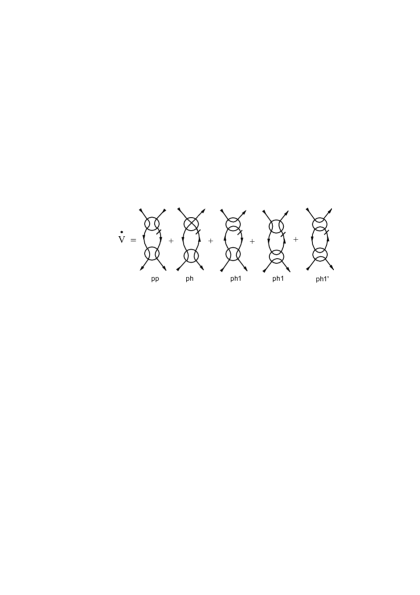
Figure 1: Diagram representation of the flow equation (IV.1). Circles denote vertices $V_{\Lambda}$, solid lines without dash correspond to Wick-ordering propagators $D_{\Lambda}$, while the lines with dash denote the single-scale propagators $F_{\Lambda}$. The lines inside vertices show direction of spin conservation.

We parametrize the vertices $V_{i_{1..4}}(\mathbf{k}_{1},\mathbf{k}_{2},\mathbf{k}_{3})$ in terms of the average momenta $\mathbf{k}_{\mathrm{pp}}=(\mathbf{k}_{1}-\mathbf{k}_{2})/2$, $\mathbf{k}_{\mathrm{ph}}=(\mathbf{k}_{2}+\mathbf{k}_{3})/2$, $\mathbf{k}_{\mathrm{ph1}}=(\mathbf{k}_{1}+\mathbf{k}_{3})/2$, and the momentum transfers $\mathbf{q}_{\mathrm{pp}}=\mathbf{k}_{1}+\mathbf{k}_{2}$, $\mathbf{q}_{\mathrm{ph}}=\mathbf{k}_{3}-\mathbf{k}_{2}$, and $\mathbf{q}_{\mathrm{ph1}}=\mathbf{k}_{1}-\mathbf{k}_{3}$ in the particle-particle and particle-hole channels. For convenience we decompose vertex functions into the contributions of the corresponding channels. Written explicitly, our parametrization reads

$$V_{i_{1..4},\Lambda}(\mathbf{k}_{1},\mathbf{k}_{2},\mathbf{k}_{3}) =V_{i_{1..4},\Lambda}^{\mathrm{pp}}(\mathbf{k}_{\mathrm{pp}},\mathbf{k}_{\mathrm{pp}}-\mathbf{q}_{\mathrm{ph1}},\mathbf{q}_{\mathrm{pp}})$$

$$+V_{i_{1..4},\Lambda}^{\mathrm{ph}}(\mathbf{k}_{\mathrm{ph}}+\mathbf{q}_{\mathrm{ph1}},\mathbf{k}_{\mathrm{ph}},\mathbf{q}_{\mathrm{ph}})$$

$$+V_{i_{1..4},\Lambda}^{\mathrm{ph1}}(\mathbf{k}_{\mathrm{ph1}},\mathbf{k}_{\mathrm{ph1}}-\mathbf{q}_{\mathrm{ph}},\mathbf{q}_{\mathrm{ph1}}).$$ (29)

The first two arguments of functions $V_{i_{1..4}}^{\mathrm{pp,ph}}$ correspond to the average incoming and outgoing momentum, while the third argument denotes the momentum transfer.

The functions $V_{i_{1..4},\Lambda}^{\mathrm{pp},\mathrm{ph}}$ of three continuum $2$-component variables is hard to treat accurately numerically. For $\mathrm{ph1}$ channel we pick out renormalized Coulomb interaction

$$V_{i_{1..4},\Lambda}^{\mathrm{ph1}}(\mathbf{k}_{\mathrm{ph1}},\mathbf{k}_{\mathrm{ph1}}-\mathbf{q}_{\mathrm{ph}},\mathbf{q}_{\mathrm{ph1}})$$

$$= \widetilde{V}_{i_{1..4},\Lambda}^{\mathrm{ph1}}(\mathbf{k}_{\mathrm{ph1}},\mathbf{k}_{\mathrm{ph1}}-\mathbf{q}_{\mathrm{ph}},\mathbf{q}_{\mathrm{ph1}})$$

$$+ \frac{2\pi\alpha}{\Pi_{\Lambda}(\mathbf{q}_{\mathrm{ph1}})}g_{\Lambda,\mathbf{k}_{\mathrm{ph1}},\mathbf{q}_{\mathrm{ph1}}}^{i_{1}i_{3}}g_{\Lambda,\mathbf{k}_{\mathrm{ph1}}-\mathbf{q}_{\mathrm{ph}},\mathbf{q}_{\mathrm{ph1}}}^{i_{2}i_{4}}$$

by introducing the renormalized polarization $\Pi(\mathbf{q})$ and electron-electric field vertex $g_{\Lambda,\mathbf{k},\mathbf{q}}$ functions. We then approximate the functions $V_{i_{1..4},\Lambda}^{\mathrm{pp},\mathrm{ph}}$ and $\widetilde{V}_{i_{1..4},\Lambda}^{\mathrm{ph1}}$ neglecting their dependence on their third argument (i.e. transfer momenta $\mathbf{q}_{\mathrm{pp}}$, $\mathbf{q}_{\mathrm{ph}},$ or $\mathbf{q}_{\mathrm{ph1}}$), which are assumed to be zero in the actual calculation of these quantities. The justification for this approximation is that at finite $\mathbf{k},\mathbf{k}^{\prime}$ the dependence of these functions on $\mathbf{q}_{\mathrm{pp,ph}}$ is non-singular, while there is an essential singularity of the considering functions on the first two momenta, $V_{i_{1..4},\Lambda}^{\mathrm{ph}}(\mathbf{k},\mathbf{k}^{\prime},\mathbf{0})\mathbf{\sim}\max(\Lambda,\mathbf{|k|,|k}^{\prime}\mathbf{|)}^{\gamma-1}$ $\times\max(\Lambda,\min(\mathbf{|k|,|k}^{\prime}\mathbf{|))}^{-\gamma}$. We have also verified that taking into account the full momentum dependence of $V_{i_{1..4},\Lambda}^{\mathrm{pp},\mathrm{ph}}$ and $\widetilde{V}_{i_{1..4},\Lambda}^{\mathrm{ph1}}$ yields only small corrections to the obtained results.

To treat accurately the remaining momentum dependences, we follow the idea of Ref. Salmhofer1 , expanding these functions in some basis. Since the dependence on the absolute value of first two arguments is expected to be singular (as follows from the analysis of Sect. II), we expand in Fourier harmonics with respect to the angle of each of the two momenta. The resulting flow equations for $V_{i_{1..4},\Lambda}^{\mathrm{pp},\mathrm{ph}}$, $\widetilde{V}_{i_{1..4},\Lambda}^{\mathrm{ph1}}$, $g_{\Lambda,\mathbf{k},\mathbf{q}}$, and $\Pi_{\Lambda}(\mathbf{q})$ are presented in the Appendix B.

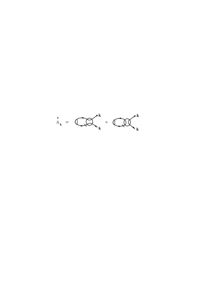
Figure 2: Diagram representation of the flow equation for the triangular vertex $\Delta_{\mathbf{k},\Lambda}$ (denoted as triangles in the right-hand side). The first (both) term(s) in the right-hand side are respectively included for the spin (charge) vertex. The notations are the same, as in Fig. 1.

To calculate the chiral spin or charge susceptibility, we first calculate the flow of the triangular vertex $\Delta_{\mathbf{k},\Lambda}$ according to the diagrams of Fig. 2. The susceptibility is then obtained straightforwardly by convolution of two triangular vertices with two Green functions.

The flow is started at $\Lambda=\Lambda_{\mathrm{uv}}>1/v_{F},$ and finished for some $\Lambda=\Lambda_{\min}\ll v_{F}.$  The bare value of the vertex corresponds to the bare Coulomb interaction

$$g_{\Lambda_{\mathrm{uv}},\mathbf{k},\mathbf{q}}^{i_{1}i_{2}} = (\gamma_{0})_{i_{1}i_{2}},$$

$$\Pi_{\Lambda_{\mathrm{uv}}}(\mathbf{q}) = |\mathbf{q}|,$$

$$V_{i_{1..4},\Lambda_{\mathrm{uv}}}^{\mathrm{pp}} = V_{i_{1..4},\Lambda_{\mathrm{uv}}}^{\mathrm{ph}}=\widetilde{V}_{i_{1..4},\Lambda_{\mathrm{uv}}}^{\mathrm{ph1}}=0,$$

$$\Delta^{i_{1},i_{2}}_{\mathbf{k},\Lambda_{\mathrm{uv}}} = \delta_{i_{1},i_{2}}.$$ (31)

IV.2 Results

IV.2.1 Flow without the Fermi velocity renormalization

First we neglect the self-energy effects by putting $\Sigma=0.$ In the absence of self-energy effects, all the vertices have dimension $k^{-1},$ and can be expressed in terms of the scaling functions

$$V_{i_{1..4},m,n,\Lambda}^{\mathrm{pp,ph,ph}^{\prime}}(|\mathbf{k|},|\mathbf{k}^{\prime}|) = \frac{1}{|\mathbf{k|}}f_{i_{1}..i_{4},m,n}^{\mathrm{pp},\mathrm{ph,ph}^{\prime}}\left(\frac{|\mathbf{k}^{\prime}|}{|\mathbf{k}|},\frac{\Lambda}{|\mathbf{k}|},\frac{\Lambda_{\text{uv}}}{|\mathbf{k}|}\right),$$

$$\Pi_{\Lambda}(\mathbf{q}) = |\mathbf{q|}f^{\mathrm{\Pi}}\left(\frac{\Lambda}{|\mathbf{q}|},\frac{\Lambda_{\text{uv}}}{|\mathbf{q}|}\right),$$ (32)

$$g_{\Lambda,\mathbf{k},\mathbf{q}}^{i_{1}i_{2}} = f_{i_{1},i_{2},m,n}^{\mathrm{g}}\left(\frac{|\mathbf{k}|}{|\mathbf{q}|},\frac{\Lambda}{|\mathbf{q}|},\frac{\Lambda_{\text{uv}}}{|\mathbf{q}|}\right)$$

where $m,n$ numerates Fourier harmonics with respect to the directions of momenta $\mathbf{k}$, $\mathbf{k}^{\prime},$ or $\mathbf{q}$. For sufficiently large $\Lambda_{\text{uv}}\sim 1/v_{F}$ and small momenta, one can ignore the last argument in these scaling functions.

The flow of $V^{\mathrm{ph}}(\mathbf{k,k}^{\prime})$ alone (with zero interactions $V^{\mathrm{pp},\mathrm{ph1}^{\prime}}$) reproduces the results of the ladder approach of Sect. II. We obtain the critical value $\alpha_{r}^{cr}=3.0/(2\pi)$ which is close to the value $\alpha_{r}^{cr}=2.9/(2\pi)$, obtained in Refs. Khveschenko1 ; Murthy ; Gusynin , the difference is related to the discretization of momentum dependence of the vertices. The flow of $\Pi(\mathbf{q})$ alone reproduces (in the end of the flow) the renormalization of the dielectric constant by the static polarization bubble, described by the Eq. (5),

$$f^{\mathrm{\Pi}}\left(0,\infty\right)=Z_{D}=1+\pi\alpha/2.$$ (33)

Figure 3: Scale dependence of the absolute value of the vertex functions $|\mathbf{k|}V_{i_{1..4},m,n,\Lambda}^{\mathrm{pp,ph,ph1}}(|\mathbf{k|},|\mathbf{k}|)$ (a,c), the renormalized Coulomb interaction $\alpha_{R,\Lambda}(\mathbf{q})$, and the electron-electric field interaction vertex $g_{\Lambda,\mathbf{0},\mathbf{q}}^{1,1}$ (b,d) for $\alpha=4/(2\pi)$ (a,b) and $\alpha=5.5/(2\pi)$ (c,d). Vertices pp,ph,ph1 correspond to the intrasublattice interaction $i_{1..4}=1$, while $\mathrm{pp}^{\prime}$,$\mathrm{ph^{\prime}}$ correspond to the intersublattice interaction $i_{1}=i_{3}=1,i_{2}=i_{4}=2$.

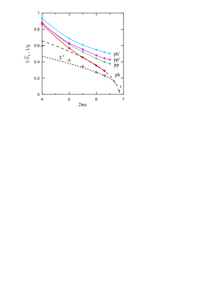
Figure 4: (Color online) Interaction dependence of the absolute value of inverse small momentum s-wave components of the dimensionless vertex functions $\overline{V}_{0,i_{1..4},0,0}^{\mathrm{pp,ph}}$ and inverse charge susceptibility in the end of the flow. Long-dashed line corresponds to the fit of ph vertex function by the dependence $A_{V}/\sqrt{\alpha_{c,V}-\alpha}$, long-dashed line corresponds to the fit of the inverse susceptibility by $\chi^{-1}=A_{\chi}(1+B_{\chi}\sqrt{\alpha_{c,\chi}-\alpha})^{2}$. The other notations are the same as in Fig. 3.

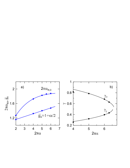
Figure 5: (Color online) Interaction dependence of the renormalized Coulomb interaction $\alpha_{R,0}$, the electron-electric field interaction vertex $\overline{g}_{0}^{1,1}$ (a), and the exponents of the momentum dependence of the vertices $\gamma_{V,\chi}$ (b) is shown by points. Upper solid line in (a) corresponds to the weak-coupling result (34) of Ref. Sodemann , while lower solid line corresponds to the linear dependence $1+\alpha/2$; solid line in (b) is the result of the fit coording to the Eq. (35)

In the present paper we consider however the combined contribution of all the channels. To analyze the results, we plot dimensionless vertices $\overline{V}_{\Lambda,i_{1}..i_{4},0,0}^{\mathrm{pp,ph,ph1}}(|\mathbf{k|})=|\mathbf{k|}V_{i_{1..4},0,0,\Lambda}^{\mathrm{pp,ph,ph1}}(|\mathbf{k|},|\mathbf{k}|)$ as functions of $\Lambda/|\mathbf{k}|,$ coupling constants $\alpha_{R,\Lambda}(|\mathbf{q|})=\alpha|\mathbf{q|}/\Pi_{\Lambda}(|\mathbf{q|}),$ and the vertex functions $g_{\Lambda,\mathbf{0},\mathbf{q}}^{i_{1}i_{2}}$ as functions of $\Lambda/|\mathbf{q}|$ (see Fig. 3). We see, that the scaling forms (32) are approximately fulfilled. For small $\alpha\lesssim 5/(2\pi)$ we find that the interactions, generated in the particle-particle and particle-hole channel are close to each other in the absolute value, having the opposite signs, and therefore, almost cancel each other. At the same time, for larger interactions, this cancellation is lifted, and one of the coupling constants, corresponding to the intrasublattice interaction in the particle-hole channel, becomes bigger than the other interactions.

The interaction dependence of the inverse dimensionless quantities $\overline{V}_{0,i_{1}..i_{4},m,n}^{\mathrm{pp,ph}}=\lim_{x\rightarrow 0,y\rightarrow\infty}f_{i_{1}..i_{4},m,n}^{\mathrm{pp},\mathrm{ph}}\left(1,x,y\right)$, corresponding to the limit $k\rightarrow 0,\Lambda/k\rightarrow 0\$of the coupling constants of Fig. 3, is shown in Fig. 4. We find that similarly to the ladder approach of Sect. III, the leading intrasublattice component $\overline{V}_{0,1111}^{\mathrm{ph}}$ (which is equal to $|\mathbf{k|(}\Gamma_{\mathbf{kk0}}^{0}+\Gamma_{\mathbf{kk0}}^{12})-2\pi\alpha_{r}=$ $\pi\alpha_{r}(1/\sqrt{1-2\alpha_{r}}-1)$ in the ladder case), increases faster than other components. By fitting the obtained results with the dependence $A_{V}/\sqrt{\alpha_{c,V}-\alpha}$ we find $\alpha_{c,V}=6.9/(2\pi).$ From this fit we also observe, that the ladder approximation with renormalized parameters is applicable in fact only at $\alpha>5/(2\pi),$ i.e. outside the region, where particle-particle and particle-hole channels compensate each other. The corresponding region below the critical interaction, which can be associated with the critical regime, appears to be rather narrow. Calculations of the chiral susceptibility shows that the spin and charge susceptibility are equal in the considering model, since the second contribution in the right-hand side of Fig. 2 vanishes. Similarly to previous studiesHerbut ; Honerkamp , additional short-range interactions are expected to remove this degeneracy, yielding either spin or charge order depending on the ratio of the on-site and nearest-neighbour Coulomb interaction. Since the nearest-neighbour Coulomb interaction is expected to be smaller than the on-site component, the spin-density wave is expected to be more favourable, than the charge density wave. The susceptibility, obtained within the present model, containing only long-range interaction, is not singular near the chiral phase transition, similarly to the ladder approximation. Its fit with the dependence $\chi^{-1}=A_{\chi}(1+B_{\chi}\sqrt{\alpha_{c,\chi}-\alpha})^{2},$ similar to the obtained in Eq. (24), yields $\alpha_{c,\chi}=6.7/(2\pi)$, which is somewhat smaller $\alpha_{c,V}$. The small difference between $\alpha_{c,V}$ and $\alpha_{c,\chi}$ likely occurs because of the narrowness of the region, where such fits are applicable.

We see that the critical coupling constants $\alpha_{c,V,\chi}$ are approximately twice larger, than the constant $\alpha_{rc},$ obtained in the ladder analysis. To understand the reason of this difference, we plot in Fig. 5a the renormalized coupling constant $\alpha_{R,0}=\alpha/Z_{D}^{\prime},$ where

$$Z_{D}^{\prime}=\lim_{q\rightarrow 0,\Lambda/q\rightarrow 0}\Pi_{\Lambda}(|\mathbf{q|})/|\mathbf{q|}=\lim_{x\rightarrow 0,y\rightarrow\infty}f^{\mathrm{\Pi}}\left(x,y\right),$$

and the vertex

$$\overline{g}_{0}^{i_{1}i_{2}}=\lim_{x,z\rightarrow 0,y\rightarrow\infty}f_{i_{1},i_{2},m,n}^{\mathrm{g}}\left(z,x,y\right).$$

Due to vertex corrections, we obtain $Z_{D}^{\prime}<Z_{D}$, which agrees with the observation of Ref. Kotov ; Sodemann that the vertex corrections increase the effective dielectric constant. The obtained behavior of $Z_{D}^{\prime}$ agrees well with the result of Ref. Sodemann ,

$$Z_{D}^{\prime}=Z_{D}+0.78\alpha^{2}+O(\alpha^{3}),$$ (34)

although the latter is obtained in the weak-coupling limit (second order in $\alpha$). We also find, that the interaction dependence of the intrasublattice component $\overline{g}_{0}^{11}$ is well fitted by $\overline{g}_{0}^{11}\simeq 1+\alpha/2$. This linear dependence of the vertex (with the correct coefficient) can be obtained by comparing linear and quadratic terms in Eq. (34).

From Fig. 5 we find that near chiral quantum phase transition the coupling constant renormalization factor $\alpha_{R,0}/\alpha\simeq 0.3,$ which is smaller than the ratio of the ladder and fRG critical couplings $\alpha_{rc}/\alpha_{c}\simeq 0.43$. This difference can be attributed to the vertex corrections. Although some vertex corrections (yielding suppression of the Coulomb interaction) are already accounted by Eq. (34), one should take into account, that when constructing a particle-hole ladder, in the presence of the vertex corrections each Coulomb line acquires a factor $g^{2}$. We find, that $(\overline{g}_{0}^{11})^{2}\simeq 2.25$ near the chiral phase transition. This itself would yield two times decrease of the critical interaction, which would be therefore equal $\alpha_{rc}/0.3/2.25\simeq 0.68,$ somewhat smaller than the obtained value $\alpha_{c}.$ The remaining difference can be explained by partial compensation between particle-hole and the particle-particle channel near quantum phase transition.

From Fig. 3c one can see that at $\alpha$ close to chiral phase transition, the dimensionless coupling constants do not saturate yet in the considered range of $\Lambda/q$ (the same behavior is observed for susceptibilities, which are not shown). Considering smaller $\Lambda$ requires increasing number of discretization points, and not feasible numerically. Apart from that, some deviations from scaling are observed, which may be attributed to the discretization procedure. To determine critical Coulomb interaction more accurately, we determine the exponents $\gamma_{V}$ and $\gamma_{\chi},$ defined by

$$V_{i_{1..4},0,0,\Lambda}^{\mathrm{ph}}(|\mathbf{k|},|\mathbf{k}^{\prime}|) = \frac{B_{V}(k^{\prime})}{k^{\gamma_{V}}},\text{ }k^{\prime}<\Lambda<k,$$

$$\Delta_{\mathbf{k},\Lambda} = \frac{B_{\chi}(k)}{\Lambda^{\gamma_{\chi}}},\ \ k<\Lambda$$ (35)

These exponents can be determined in the whole range $\Lambda\ll 1$ and do not require achieving saturation of the coupling constants. In the ladder approach one has $1-\gamma_{V}=$ $\gamma_{\chi}=\gamma.$ The results of the renormalization-group calculation are shown in Fig. 5b. We see that the exponents $\gamma_{V},$ $\gamma_{\chi}$ also behave similarly to the ladder approach for $2\pi\alpha>5,$ and show a bifurcation point at $\alpha_{c}=1.048\pm 0.008.$ We consider this result as an estimate for the critical coupling strength. This is much smaller than the value $\alpha_{c}=1.62$ in the ladder approximation, and agrees well with the results of Monte-Carlo analysis MC .

IV.2.2 Flow with the Fermi velocity renormalization

Figure 6: Scale dependence of the absolute value of the vertex functions $|\mathbf{k|}V_{i_{1..4},m,n,\Lambda}^{\mathrm{pp,ph,ph1}}(|\mathbf{k|},|\mathbf{k}|)$ (a,c), the renormalized Coulomb interaction $\alpha_{R,\Lambda}(\mathbf{q})$, and the electron-electric field interaction vertex $g_{\Lambda,\mathbf{0},\mathbf{q}}^{1,1}$ (b,d) for $\alpha=16/(2\pi)$ (a,b) and $\alpha=20/(2\pi)$ (c,d) with account of the Fermi velocity renormalization. The notations are the same, as in Fig. 3.

Figure 7: Interaction dependence of the absolute value of inverse small momentum s-wave components of the dimensionless vertex functions $\overline{V}_{0,\{1,1,1,1\},0,0}^{\mathrm{ph}}$ (line and points) and inverse charge susceptibility (crosses) in the end of the flow with account of the renormalization of the Fermi velocity. Long-dashed line corresponds to the extrapolation of interaction dependence of the inverse vertex.

To model the effect of Fermi velocity renormalization, we put $\Sigma(k)=(\alpha/4)v_{F}\gamma_{a}k_{a}\ln(\Lambda_{uv}/|\mathbf{k|})$. The scale dependences of the vertex functions are shown in Fig. 6. As one can expect, the universality of the scaling functions is violated by renormalization of the Fermi velocity. Due to relatively large Coulomb interaction, the contributions of the particle-particle and particle-hole channels are split, such that the above discussed compensation of the two contributions is less pronouced. The electron-electric field vertex renormalization achieves values $\gamma\simeq 1.5,$ which are comparable to those obtained in the previous subsection without Fermi velocity renormalization (although for larger interaction strength), strongly suppressing the critical interactions. The dependence of the interaction in the end of the flow on the coupling constants is shown in Fig. 7. We obtain the critical coupling constant $\alpha_{c}^{v}=3.7,$ while without the vertex corrections in the Bethe-Salpeter approach the chiral instability does not occur in the static approximation with the Fermi velocity renormalizationPopovici . Apart from the vertex corrections, discussed in previous Section, the reason of getting finite and not large critical interaction is in the renormalization of Fermi velocity also when calculating the polarization bubble. This effect was not accounted in Ref. Popovici, and reduces the screening of the interaction, decreasing therefore the effective interaction. To see more explicitly the effect of changing screening in the presence of the renormalization of the Fermi velocity, we switch off the renormalization of the Fermi velocity in the polarization bubble $\Pi_{\Lambda}(\mathbf{q})$ and obtain $\alpha_{c}^{v,0}=4.6$ which is somewhat higher than the $\alpha_{c}^{v},$ but yet finite and even considerably smaller than the result of Ref. Popovici, with dynamic effects included. Therefore, we conclude that even with the Fermi velocity renormalization, vertex corrections yield substantial decrease of the critical interaction. The obtained value $\alpha_{c}^{v}=3.7$ is expected to be further reduced by the effects of dynamic screening of Coulomb interaction, which may yield the critical Coulomb interactrion comparable to the one in suspended graphene.

V Conclusion

In the present paper we have analyzed the results of the Bethe-Salpeter (ladder) approximation and the functional renormalization-group approach, which accounts for all the channels of electron interaction to describe chiral phase transition in a system of Dirac electrons. We have shown, that without the Fermi velocity renormalization, at sufficiently small coupling constants $\alpha<5/(2\pi)$ the particle-particle and particle-hole channels partly compensate each other. On the other hand, for $\alpha>5/(2\pi)$ the compensation is not present, and the particle-hole channel dominates. This yields chiral phase transition at $\alpha_{c}=1.05,$ which properties are rather similar to those, obtained in the Schwinger-Dyson or Bethe-Salpeter (ladder) analysis. The vertex corrections enhance the tendency towards chiral symmetry breaking and compensate the effect of partial cancellation between the particle-particle and particle-hole channels.

With accounting the Fermi velocity renormalization, the abovementioned compensation is weakened, and therefore vertex corrections are expected to have even stronger effect on the critical interaction sterngth. In particular, in the static approximation we obtain $\alpha_{c}^{v}=3.7$, while this value is expected to be further reduced by the effects of dynamic screening of Coulomb interaction, yielding the results for the critical Coulomb interaction smaller than previous estimates. Whether it remains above or below the experimental $\alpha=2.2$ and how much it differs from the results of Monte-Carlo analysis, requires additional studies. As also described in the introduction, the effect of the other bands, which add short-range interactions on the top of the long-range Coulomb tail, can be also important. Their analysis is beyond of the scope of the present work, and is interesting to be performed in the future. Finally, the effect of impurities, either neutral, or charged, in the presence of the interelectron Coulomb interaction, has to be analyzed.

Acknowledgements. The author is grateful to M. Scherer, F. Assaad, M. I. Katsnelson, M. Titov, S. Friedrich, and C. Wetterich for discussions. The work is supported by FASO Russian Federation (theme ”Electron” No. 01201463326), grant of the Dynasty foundation, and Act 211 Government of the Russian Federation, contract 02.A03.21.0006. The calculations are performed using computer cluster Uran of Ural branch RAS.

Appendix. A. Solution of the Bethe-Salpeter equation for the vertex

Substituting the ansatz (11) into the Eq. (10) we find

$$\left(\Gamma_{\mathbf{kk}^{\prime}\mathbf{0}}^{0}-\frac{2\pi\alpha}{|\mathbf{k}-\mathbf{k}^{\prime}|}\right)\gamma_{0}\otimes\gamma_{0}+\Gamma_{\mathbf{kk}^{\prime}\mathbf{0}}^{1}\gamma_{a}\otimes\gamma_{a}$$

$$+\Gamma_{\mathbf{kk}^{\prime}\mathbf{0}}^{12}i\gamma_{0}\gamma_{1}\gamma_{2}\otimes i\gamma_{0}\gamma_{0}\gamma_{1}\gamma_{2}$$

$$= \frac{\alpha_{r}}{4}\int\frac{dpd\theta_{p}}{2\pi}\frac{1}{|\mathbf{p}-\mathbf{k|}}\left[I\otimes I-\frac{p_{a}p_{b}}{|\mathbf{p}|^{2}}\gamma_{0}\gamma_{a}\otimes\gamma_{0}\gamma_{a}\right]$$

$$\times \left[\Gamma_{\mathbf{pk}^{\prime}\mathbf{0}}^{0}\gamma_{0}\otimes\gamma_{0}+\Gamma_{\mathbf{pk}^{\prime}\mathbf{0}}^{1}\gamma_{b}\otimes\gamma_{b}\right.$$

$$+\left.\Gamma_{\mathbf{pk}^{\prime}\mathbf{0}}^{12}i\gamma_{0}\gamma_{1}\gamma_{2}\otimes i\gamma_{0}\gamma_{1}\gamma_{2}\right].$$

In the following we consider the ”s-wave” component of the vertex, which is obtained by averaging over the directions of $\mathbf{k}$ and $\mathbf{k}^{\prime}.$ For this component, which we refer in the following as $\Gamma_{kk^{\prime}}^{m},$ we obtain,

$$\left[\Gamma_{kk^{\prime}}^{0}-\frac{2\pi\alpha}{k_{>}}K_{1}\left(\frac{k_{<}}{k_{>}}\right)\right]\gamma_{0}\otimes\gamma_{0}+\Gamma_{kk^{\prime}}^{1}\gamma_{a}\otimes\gamma_{a}$$

$$+\Gamma_{kk^{\prime}}^{12}i\gamma_{0}\gamma_{1}\gamma_{2}\otimes i\gamma_{0}\gamma_{0}\gamma_{1}\gamma_{2}$$

$$= \frac{\alpha_{r}}{4}\int\frac{dp}{(p,k)_{>}}K_{1}\left(\frac{(p,k)_{<}}{(p,k)_{>}}\right)\left[I\otimes I-\frac{1}{2}\gamma_{0}\gamma_{a}\otimes\gamma_{0}\gamma_{a}\right]$$

$$\times \left[\Gamma_{pk^{\prime}}^{0}\gamma_{0}\otimes\gamma_{0}+\Gamma_{pk^{\prime}}^{1}\gamma_{b}\otimes\gamma_{b}+\Gamma_{pk^{\prime}}^{12}i\gamma_{0}\gamma_{1}\gamma_{2}\otimes i\gamma_{0}\gamma_{1}\gamma_{2}\right],$$

where $K_{1}(x)=(2/\pi)K(x),$ $K(x)$ is the complete elliptic integral of the first kind, $k_{<}=\min(k,k^{\prime})$, $k_{>}=\max(k,k^{\prime}),$ $(p,k)_{>}=\max(p,k),$ $(p,k)_{<}=\min(p,k)$. Performing matrix multiplication, we obtain Eq. (12) of the main text.

With the anzatz (III) for the linear combinations (13), we obtain for the functions $g_{m}(x)$ with $m=s,a$ the equations

$$\frac{1}{k}g_{m}(\frac{k^{\prime}}{k}) = \frac{2\pi\alpha_{r}}{k}K\left(\frac{k^{\prime}}{k}\right)+\frac{\alpha_{r}r_{m}}{4kk^{\prime}}\int_{0}^{k^{\prime}}dpg_{m}\left(\frac{p}{k^{\prime}}\right)K_{1}\left(\frac{p}{k}\right)$$ (38)

$$+\frac{\alpha_{r}r_{m}}{4k}\int_{k^{\prime}}^{k}\frac{dp}{p}g_{m}\left(\frac{k^{\prime}}{p}\right)K_{1}\left(\frac{p}{k}\right)$$

$$+\frac{\alpha_{r}}{4}\int_{k}^{\Lambda}\frac{dp}{p^{2}}g_{m}\left(\frac{k^{\prime}}{p}\right)K_{1}\left(\frac{k}{p}\right).$$

Supposing the last integral is convergent at $\Lambda\rightarrow\infty$, these equations can be rewritten as

$$g_{m}(x) = 2\pi\alpha_{r}K_{1}\left(x\right)+\frac{\alpha_{r}r_{m}}{4}\int_{0}^{1}d\widetilde{p}g_{m}(\widetilde{p})K_{1}\left(\widetilde{p}x\right)$$ (39)

$$+\frac{\alpha_{r}r_{m}}{4}\int_{x}^{1}\frac{d\widetilde{p}}{\widetilde{p}}g_{m}(\widetilde{p})K_{1}\left(\frac{x}{\widetilde{p}}\right)$$

$$+\frac{\alpha_{r}r_{m}}{4x}\int_{0}^{x}d\widetilde{p}g_{m}(\widetilde{p})K_{1}\left(\frac{\widetilde{p}}{x}\right).$$

The obtained integral equation can be then transformed to the differential one,

$$x[xg_{m}(x)]^{\prime\prime}=-\frac{\alpha_{r}r_{m}}{4}g_{m}(x)$$ (40)

with

$$g_{m}(1)-2\pi\alpha=-2g_{m}^{\prime}(1)=\frac{\alpha_{r}r_{m}}{2}\int_{0}^{1}dxg_{m}(x).$$ (41)

The solution to the obtained equations has the form of the Eq. (17), of the main text, which yields

$$k_{>}\Gamma_{kk^{\prime}}^{1} = \frac{\pi\alpha_{r}}{2\sqrt{1-2\alpha_{r}}}\left(\frac{k_{>}}{k_{<}}\right)^{\gamma}-\frac{\pi\alpha_{r}}{2},$$ (42)

$$k_{>}\Gamma_{kk^{\prime}}^{0,12} = \frac{\pi\alpha_{r}}{2\sqrt{1-2\alpha_{r}}}\left(\frac{k_{>}}{k_{<}}\right)^{\gamma}$$

$$\pm \frac{\pi\alpha_{r}}{\sqrt{1-\alpha_{r}}}\left(\frac{k_{>}}{k_{<}}\right)^{\gamma_{a}}+\frac{\pi\alpha_{r}}{2},$$

where we have denoted $\gamma=\gamma_{s}=\frac{1}{2}\left(1-\sqrt{1-2\alpha_{r}}\right).$

The solution of the equations (39) beyond the approximation (16) can be obtained analytically only for $x=k^{\prime}/k\ll 1.$ Assuming again $g_{m}(x\ll 1)=A_{m}x^{-\gamma_{m}}$ we find:

$$A_{m}x^{-\gamma_{m}} = 2\pi\alpha+\frac{\alpha r_{m}}{4}\int_{0}^{1}d\widetilde{p}g_{m}(\widetilde{p})$$

$$+\frac{\alpha r_{m}}{4}\int_{x}^{1}\frac{d\widetilde{p}}{\widetilde{p}}g_{m}(\widetilde{p})K_{1}\left(\frac{x}{\widetilde{p}}\right)$$

$$+\frac{\alpha r_{m}A_{m}}{4x}\int_{0}^{x}d\widetilde{p}\widetilde{p}^{-\gamma_{m}}K_{1}\left(\frac{\widetilde{p}}{x}\right).$$

To simplify the second integral, we introduce the constant $C$ such that $x\ll C\ll 1.$ Splitting the regions of integration over $\widetilde{p}$ by the constant $C$, we find

$$A_{m}x^{-\gamma_{m}} = 2\pi\alpha_{r}+\frac{\alpha_{r}r_{m}}{4}\int_{0}^{1}d\widetilde{p}g_{m}(\widetilde{p})$$

$$+\frac{\alpha_{r}r_{m}A_{m}}{4}\int_{x}^{C}\frac{d\widetilde{p}}{\widetilde{p}^{1+\gamma_{m}}}K_{1}\left(\frac{x}{\widetilde{p}}\right)$$

$$+\frac{\alpha_{r}r_{m}}{4}\int_{C}^{1}\frac{d\widetilde{p}}{\widetilde{p}}g_{m}(\widetilde{p})$$

$$+\frac{\alpha_{r}r_{m}A_{m}}{4x}\int_{0}^{x}d\widetilde{p}\widetilde{p}^{-\gamma_{m}}K_{1}\left(\frac{\widetilde{p}}{x}\right)$$

$$= 2\pi\alpha_{r}+\frac{\alpha_{r}r_{m}}{4}\int_{0}^{1}d\widetilde{p}g_{m}(\widetilde{p})-\frac{\alpha_{r}r_{m}A_{m}}{4\gamma_{m}}$$

$$+\frac{\alpha_{r}r_{m}}{4}\int_{0}^{1}\frac{d\widetilde{p}}{\widetilde{p}}\left[g_{m}(\widetilde{p})-\frac{A_{m}}{\widetilde{p}^{\gamma_{m}}}\right]$$

$$+\frac{\alpha_{r}r_{m}A_{m}}{4x^{\gamma_{m}}}\left[\int_{0}^{1}dyy^{-\gamma_{m}}K_{1}\left(y\right)\right.$$

$$\left.+\int_{1}^{\infty}\frac{dy}{y^{1+\gamma_{m}}}K_{1}\left(\frac{1}{y}\right)\right].$$

The resulting equation for $\gamma_{m}$ reads

$$1=\frac{\alpha_{r}r_{m}}{4}\int_{0}^{1}dy\left(y^{\gamma_{m}-1}+y^{-\gamma_{m}}\right)K\left(y\right);$$ (45)

the result for the exponent $\gamma=\gamma_{s}$ coincides with that obtained in the fall on the center problemGusynin . For the constant $A_{m}$ we obtain the equation

$$\frac{\alpha_{r}r_{m}A_{m}}{4\gamma_{m}}-\frac{\alpha_{r}r_{m}}{4}\int_{0}^{1}d\widetilde{p}g_{m}(\widetilde{p})$$

$$-\frac{\alpha_{r}r_{m}}{4}\int_{0}^{1}\frac{d\widetilde{p}}{\widetilde{p}}\left[g_{m}(\widetilde{p})-\frac{A_{m}}{p^{\gamma_{m}}}\right]\begin{array}[]{c}=\end{array}2\pi\alpha$$ (47)

which can be solved numerically. Qualitatively, the solution do not differ from the simplified result (42).

Similar consideration can be performed for the triangular vertex, considered in Ref. Gusynin1 , cf. also main text. The corresponding equation for the ”s-wave” component of the vertex reads

$$\Delta_{p}=\Delta_{0}+\frac{\alpha_{r}}{2}\int\limits_{0}^{\Lambda}\frac{dk}{(k,p)_{>}}K_{1}\left(\frac{(k,p)_{<}}{(k,p)_{>}}\right)\Delta_{k},$$ (48)

where $\Delta_{0}$ is the bare value of the triangular vertex. Substituting $\Delta_{p}=Ap^{-\gamma}$ for $p\ll\Lambda$ and introducing $p\ll C\ll\Lambda,$ we obtain for $\gamma$ the equation

$$Ap^{-\gamma} = \Delta_{0}+\frac{\alpha_{r}A}{2p}\int\limits_{0}^{p}\frac{dk}{k^{\gamma}}K_{1}\left(\frac{k}{p}\right)$$

$$+\frac{\alpha_{r}A}{2}\int\limits_{p}^{C}\frac{dk}{k^{1+\gamma}}K_{1}\left(\frac{p}{k}\right)+\frac{\alpha_{r}}{2}\int\limits_{C}^{\Lambda}\frac{dk}{k}\Delta_{k}$$

$$= \Delta_{0}+\frac{\alpha_{r}A}{2p^{\gamma}}\left[\int\limits_{0}^{1}\frac{dy}{y^{\gamma}}K_{1}\left(y\right)+\int\limits_{1}^{\infty}\frac{dk}{y^{1+\gamma}}K_{1}\left(\frac{1}{y}\right)\right]$$

$$+\frac{\alpha_{r}}{2}\int\limits_{0}^{\Lambda}\frac{dk}{k}\left(\Delta_{k}-\frac{A}{k^{\gamma}}\right)-\frac{\alpha_{r}A\Lambda^{\gamma}}{2\gamma}.$$

From this we find again $\gamma=\gamma_{s},$ determined above, and the constant $A$ is determined by

$$\frac{\alpha_{r}A\Lambda^{\gamma}}{2\gamma}-\frac{\alpha_{r}}{2}\int\limits_{0}^{\Lambda}\frac{dk}{k}\left(\Delta_{k}-\frac{A}{k^{\gamma}}\right)=\Delta_{0}.$$ (50)

With the approximation (16) this reduces to the result (23) of the main text.

Appendix. B. Functional renormalization group equations

In this Appendix we present analytical form of the renormalization-group equations, shown in Fig. 1 of the paper. The equation for the vertices $V_{i_{1..4}}^{m}(\mathbf{k}_{1},\mathbf{k}_{2},\mathbf{k}_{3})$ in the static approximation reads:

$$\dot{V}_{i_{1..4},\Lambda}(\mathbf{k}_{1},\mathbf{k}_{2},\mathbf{k}_{3})=-\sum\limits_{\mathbf{k,}i_{1..4}^{\prime}}$$

$$\left\{V_{i_{1}i_{4}^{\prime}i_{1}^{\prime}i_{4},\Lambda}(\mathbf{k}_{1},\mathbf{k-q}_{\mathrm{ph}},\mathbf{k})V_{i_{3}^{\prime}i_{2}i_{3}i_{2}^{\prime},\Lambda}(\mathbf{k},\mathbf{k}_{2},\mathbf{k}_{3})\right.$$

$$\times\widetilde{\Pi}_{\Lambda,\mathrm{ph}}^{i_{1}^{\prime}i_{2}^{\prime};i_{3}^{\prime}i_{4}^{\prime}}(\mathbf{k},\mathbf{q}_{\mathrm{ph}})$$

$$+V_{i_{1}i_{2}i_{1}^{\prime}i_{2}^{\prime},\Lambda}(\mathbf{k}_{1},\mathbf{k}_{2},\mathbf{k})V_{i_{3}^{\prime}i_{4}^{\prime}i_{3}i_{4},\Lambda}(\mathbf{k},-\mathbf{k}+\mathbf{q}_{\mathrm{pp}},\mathbf{k}_{3})$$

$$\times\widetilde{\Pi}_{\Lambda,\mathrm{pp}}^{i_{1}^{\prime}i_{2}^{\prime};i_{3}^{\prime}i_{4}^{\prime}}(\mathbf{k},\mathbf{q}_{\mathrm{pp}})+$$

$$\left[V_{i_{1}i_{1}^{\prime}i_{3}^{\prime}i_{3},\Lambda}(\mathbf{k}_{1},\mathbf{k}-\mathbf{q}_{\mathrm{ph1}},\mathbf{k})V_{i_{4}^{\prime}i_{2}i_{2}^{\prime}i_{4},\Lambda}(\mathbf{k},\mathbf{k}_{2},\mathbf{k-q}_{\mathrm{ph}})\right.$$

$$+V_{i_{1}i_{1}^{\prime}i_{3}i_{3}^{\prime},\Lambda}(\mathbf{k}_{1},\mathbf{k}-\mathbf{q}_{\mathrm{ph1}},\mathbf{k}_{3})V_{i_{4}^{\prime}i_{2}i_{4}i_{2}^{\prime},\Lambda}(\mathbf{k},\mathbf{k}_{2},\mathbf{k}_{2}+\mathbf{q}_{\mathrm{ph1}})$$

$$\left.-2V_{i_{1}i_{1}^{\prime}i_{3}i_{3}^{\prime},\Lambda}(\mathbf{k}_{1},\mathbf{k}-\mathbf{q}_{\mathrm{ph1}},\mathbf{k}_{3})V_{i_{4}^{\prime}i_{2}i_{2}^{\prime}i_{4},\Lambda}(\mathbf{k},\mathbf{k}_{2},\mathbf{k-q}_{\mathrm{ph}})\right]$$

$$\left.\times\widetilde{\Pi}_{\Lambda,\mathrm{ph}}^{i_{2}^{\prime}i_{3}^{\prime};i_{1}^{\prime}i_{4}^{\prime}}(\mathbf{k},\mathbf{q}_{\mathrm{ph1}})\right\}.$$ (51)

where $\mathbf{k}_{\mathrm{pp}}=(\mathbf{k}_{1}-\mathbf{k}_{2})/2$ and $\mathbf{k}_{\mathrm{ph}}=(\mathbf{k}_{2}+\mathbf{k}_{3})/2$ are the average momenta in the particle-particle and the particle-hole channels, $\mathbf{q}_{\mathrm{ph1}}=\mathbf{k}_{1}-\mathbf{k}_{3}$ and the momentum transfer in the latter two channels, $\mathbf{q}_{\mathrm{pp}}=\mathbf{k}_{1}+\mathbf{k}_{2}$ and $\mathbf{q}_{\mathrm{ph}}=\mathbf{k}_{3}-\mathbf{k}_{2}.$ Using decomposition (29), we obtain the equation for the contribution of the particle-partice channel

$$\dot{V}_{i_{1..4}}^{\mathrm{pp}}(\mathbf{k,k}^{\prime},\mathbf{q})=$$ (52)

$$\sum\limits_{i_{1..4},\mathbf{k}^{\prime\prime}}\widetilde{\Pi}_{\Lambda,\mathrm{pp}}^{i_{1}^{\prime}i_{2}^{\prime};i_{3}^{\prime}i_{4}^{\prime}}(\mathbf{k},\mathbf{q})\left[V_{i_{1}i_{2}i_{1}^{\prime}i_{2}^{\prime}}^{\mathrm{pp}}(\mathbf{k,k}^{\prime\prime},\mathbf{q})\right.$$

$$+V_{i_{1}i_{2}i_{1}^{\prime}i_{2}^{\prime}}^{\mathrm{ph}}\left(\frac{\mathbf{k-k}^{\prime\prime}+\mathbf{q}}{2},\frac{\mathbf{k}^{\prime\prime}-\mathbf{k+q}}{2},\mathbf{k}+\mathbf{k}^{\prime\prime}\right)$$

$$\left.+V_{i_{1}i_{2}i_{1}^{\prime}i_{2}^{\prime}}^{\mathrm{ph1}}\left(\frac{\mathbf{k+k}^{\prime\prime}+\mathbf{q}}{2},-\frac{\mathbf{k}+\mathbf{k^{\prime\prime}-q}}{2},\mathbf{k-k}^{\prime\prime}\right)\right]$$

$$\times\left[V_{i_{3}^{\prime}i_{4}^{\prime}i_{3}i_{4}}^{\mathrm{pp}}(\mathbf{k}^{\prime\prime},\mathbf{k}^{\prime},\mathbf{q})\right.$$

$$+V_{i_{3}^{\prime}i_{4}^{\prime}i_{3}i_{4}}^{\mathrm{ph}}\left(\frac{\mathbf{k}^{\prime\prime}-\mathbf{k}^{\prime}+\mathbf{q}}{2},\frac{\mathbf{k}^{\prime}-\mathbf{k}^{\prime\prime}+\mathbf{q}}{2}\right)$$

$$\left.+V_{i_{3}^{\prime}i_{4}^{\prime}i_{3}i_{4}}^{\mathrm{ph1}}\left(\frac{\mathbf{k}^{\prime}\mathbf{+k}^{\prime\prime}+\mathbf{q}}{2},-\frac{\mathbf{k}^{\prime}+\mathbf{k^{\prime\prime}-q}}{2},\mathbf{k}^{\prime\prime}-\mathbf{k}^{\prime}\right)\right],$$

and the particle-hole channel,

$$\dot{V}_{i_{1..4}}^{\mathrm{ph}}(\mathbf{k,k}^{\prime},\mathbf{q})=\sum\limits_{i_{1..4}^{\prime},\mathbf{k}^{\prime\prime}}\widetilde{\Pi}_{\Lambda,\mathrm{pp}}^{i_{1}^{\prime}i_{2}^{\prime};i_{3}^{\prime}i_{4}^{\prime}}(\mathbf{k}^{\prime\prime},\mathbf{q})$$ (53)

$$\times\left[V_{i_{1}i_{4}^{\prime}i_{1}^{\prime}i_{4}}^{\mathrm{pp}}\left(\frac{\mathbf{k}-\mathbf{k}^{\prime\prime}+\mathbf{q}}{2},\frac{\mathbf{k}^{\prime\prime}-\mathbf{k+q}}{2},\mathbf{k}+\mathbf{k}^{\prime\prime}\right)\right.$$

$$+V_{i_{1}i_{4}^{\prime}i_{1}^{\prime}i_{4}}^{\mathrm{ph}}(\mathbf{k,k}^{\prime\prime},\mathbf{q})$$

$$\left.+V_{i_{1}i_{4}^{\prime}i_{1}^{\prime}i_{4}}^{\mathrm{ph1}}(\frac{\mathbf{k+k}^{\prime\prime}+\mathbf{q}}{2},\frac{\mathbf{k}+\mathbf{k^{\prime\prime}-q}}{2},\mathbf{k-k}^{\prime\prime})\right]$$

$$\times\left[V_{i_{3}^{\prime}i_{2}i_{3}i_{2}^{\prime}}^{\mathrm{pp}}\left(\frac{\mathbf{k}^{\prime\prime}-\mathbf{k}^{\prime}+\mathbf{q}}{2},\frac{\mathbf{k}^{\prime}-\mathbf{k}^{\prime\prime}+\mathbf{q}}{2}\right)\right.$$

$$+V_{i_{3}^{\prime}i_{2}i_{3}i_{2}^{\prime}}^{\mathrm{ph}}(\mathbf{k}^{\prime\prime},\mathbf{k}^{\prime},\mathbf{q})$$

$$\left.+V_{i_{3}^{\prime}i_{2}i_{3}i_{2}^{\prime}}^{\mathrm{ph1}}\left(\frac{\mathbf{k}^{\prime}\mathbf{+k}^{\prime\prime}+\mathbf{q}}{2},\frac{\mathbf{k}^{\prime}+\mathbf{k^{\prime\prime}-q}}{2},\mathbf{k}^{\prime\prime}\mathbf{-k}^{\prime}\right)\right].$$

We represent the vertex $V^{\mathrm{ph1}}$ according to the Eq. (IV.1) of the main text, and in the most part of calculations, we neglect the dependence of $V^{\mathrm{pp,ph}}$ and $\widetilde{V}^{\mathrm{ph1}}$ on the third argument (as discussed in the main text), projecting it to zero. We have verified that treatment of the full momentum dependence does not change the results substantially. For the vertex $\widetilde{V}^{\mathrm{ph1}}$ we obtain the equation

$$\dot{\widetilde{V}}_{i_{1..4}}^{\mathrm{ph1}}(\mathbf{k},\mathbf{k}^{\prime},\mathbf{q})\begin{array}[]{c}=\end{array}\sum\limits_{i_{1..4}^{\prime},\mathbf{k}^{\prime\prime}}\widetilde{\Pi}_{\Lambda,\mathrm{ph}}^{i_{2}^{\prime}i_{3}^{\prime};i_{1}^{\prime}i_{4}^{\prime}}(\mathbf{k}^{\prime\prime},\mathbf{q})$$ (55)

$$\left\{\left[V_{i_{1}i_{1}^{\prime}i_{3}i_{3}^{\prime}}^{\mathrm{pp}}\left(\frac{\mathbf{k-k}^{\prime\prime}+\mathbf{q}}{2},\frac{\mathbf{k-k}^{\prime\prime}-\mathbf{q}}{2},\mathbf{k}+\mathbf{k}^{\prime\prime}\right)\right.\right.$$

$$+V_{i_{1}i_{1}^{\prime}i_{3}i_{3}^{\prime}}^{\mathrm{ph}}\left(\frac{\mathbf{k}+\mathbf{k}^{\prime\prime}+\mathbf{q}}{2},\frac{\mathbf{k}+\mathbf{k}^{\prime\prime}-\mathbf{q}}{2},\mathbf{k}-\mathbf{k}^{\prime\prime}\right)$$

$$\left.+\widetilde{V}_{i_{1}i_{1}^{\prime}i_{3}i_{3}^{\prime}}^{\mathrm{ph1}}(\mathbf{k},\mathbf{k}^{\prime\prime},\mathbf{q})\right]$$

$$\times\left[V_{i_{4}^{\prime}i_{2}i_{4}i_{2}^{\prime}}^{\mathrm{pp}}\left(\frac{\mathbf{k}^{\prime\prime}-\mathbf{k}^{\prime}+\mathbf{q}}{2},\frac{\mathbf{k}^{\prime}-\mathbf{k}^{\prime\prime}+\mathbf{q}}{2},\mathbf{k}^{\prime\prime}+\mathbf{k}^{\prime}\right)\right.$$

$$+V_{i_{4}^{\prime}i_{2}i_{4}i_{2}^{\prime}}^{\mathrm{ph}}\left(\mathbf{k}^{\prime\prime},\mathbf{k}^{\prime},\mathbf{q}\right)$$

$$\left.+V_{i_{4}^{\prime}i_{2}i_{4}i_{2}^{\prime}}^{\mathrm{ph1}}(\frac{\mathbf{k}^{\prime\prime}+\mathbf{k}^{\prime}+\mathbf{q}}{2},\frac{\mathbf{k}^{\prime}+\mathbf{k}^{\prime\prime}-\mathbf{q}}{2},\mathbf{k}^{\prime\prime}-\mathbf{k}^{\prime})\right]$$

$$+\left[V_{i_{1}i_{1}^{\prime}i_{3}^{\prime}i_{3}}^{\mathrm{pp}}\left(\frac{\mathbf{k-k}^{\prime\prime}+\mathbf{q}}{2},\frac{\mathbf{k}^{\prime\prime}-\mathbf{k}+\mathbf{q}}{2},\mathbf{k}+\mathbf{k}^{\prime\prime}\right)\right.$$

$$+V_{i_{4}^{\prime}i_{2}i_{4}i_{2}^{\prime}}^{\mathrm{ph}}\left(\mathbf{k},\mathbf{k}^{\prime\prime},\mathbf{q}\right)$$

$$\left.+V_{i_{1}i_{1}^{\prime}i_{3}^{\prime}i_{3}}^{\mathrm{ph1}}\left(\frac{\mathbf{k+k}^{\prime\prime}+\mathbf{q}}{2},\frac{\mathbf{k}^{\prime\prime}+\mathbf{k}-\mathbf{q}}{2},\mathbf{k-k}^{\prime\prime}\right)\right]$$

$$\times\left[V_{i_{4}^{\prime}i_{2}i_{2}^{\prime}i_{4}}^{\mathrm{pp}}\left(\frac{\mathbf{k}^{\prime\prime}-\mathbf{k}^{\prime}+\mathbf{q}}{2},\frac{\mathbf{k}^{\prime\prime}-\mathbf{k}^{\prime}-\mathbf{q}}{2},\mathbf{k}^{\prime\prime}+\mathbf{k}^{\prime}\right)\right.$$

$$+V_{i_{4}^{\prime}i_{2}i_{2}^{\prime}i_{4}}^{\mathrm{ph}}\left(\frac{\mathbf{k}^{\prime\prime}\mathbf{+k}^{\prime}+\mathbf{q}}{2},\frac{\mathbf{k}^{\prime\prime}+\mathbf{k}^{\prime}-\mathbf{q}}{2},\mathbf{k}^{\prime\prime}-\mathbf{k}^{\prime}\right)$$

$$\left.+\widetilde{V}_{i_{4}^{\prime}i_{2}i_{2}^{\prime}i_{4}}^{\mathrm{ph1}}(\mathbf{k}^{\prime\prime},\mathbf{k}^{\prime},\mathbf{q})\right]$$

$$-2\left[V_{i_{1}i_{1}^{\prime}i_{3}i_{3}^{\prime}}^{\mathrm{pp}}\left(\frac{\mathbf{k-k}^{\prime\prime}+\mathbf{q}}{2},\frac{\mathbf{k-k}^{\prime\prime}-\mathbf{q}}{2},\mathbf{k}+\mathbf{k}^{\prime\prime}\right)\right.$$

$$+V_{i_{1}i_{1}^{\prime}i_{3}i_{3}^{\prime}}^{\mathrm{ph}}\left(\frac{\mathbf{k}+\mathbf{k}^{\prime\prime}+\mathbf{q}}{2},\frac{\mathbf{k}+\mathbf{k}^{\prime\prime}-\mathbf{q}}{2},\mathbf{k}-\mathbf{k}^{\prime\prime}\right)$$

$$\left.+\widetilde{V}_{i_{1}i_{1}^{\prime}i_{3}i_{3}^{\prime}}^{\mathrm{ph1}}(\mathbf{k},\mathbf{k}^{\prime\prime},\mathbf{q})\right]$$

$$\times\left[V_{i_{4}^{\prime}i_{2}i_{2}^{\prime}i_{4}}^{\mathrm{pp}}\left(\frac{\mathbf{k}^{\prime\prime}-\mathbf{k}^{\prime}+\mathbf{q}}{2},\frac{\mathbf{k}^{\prime\prime}-\mathbf{k}^{\prime}-\mathbf{q}}{2},\mathbf{k}^{\prime\prime}+\mathbf{k}^{\prime}\right)\right.$$

$$+V_{i_{4}^{\prime}i_{2}i_{2}^{\prime}i_{4}}^{\mathrm{ph}}\left(\frac{\mathbf{k}^{\prime\prime}\mathbf{+k}^{\prime}+\mathbf{q}}{2},\frac{\mathbf{k}^{\prime\prime}+\mathbf{k}^{\prime}-\mathbf{q}}{2},\mathbf{k}^{\prime\prime}-\mathbf{k}^{\prime}\right)$$

$$\left.\left.+\widetilde{V}_{i_{4}^{\prime}i_{2}i_{2}^{\prime}i_{4}}^{\mathrm{ph1}}(\mathbf{k}^{\prime\prime},\mathbf{k}^{\prime},\mathbf{q})\right]\right\}.$$

Finally, the vertex $\gamma$ and the inverse propagator $\Pi$ are determined from

$$\dot{g} {}_{\mathbf{k},\mathbf{q}}^{i_{2}i_{4}}\begin{array}[]{c}=\end{array}\sum\limits_{i_{1..4}^{\prime},\mathbf{k}^{\prime\prime}}\widetilde{\Pi}_{\Lambda,\mathrm{ph}}^{i_{2}^{\prime}i_{3}^{\prime};i_{1}^{\prime}i_{4}^{\prime}}(\mathbf{k}^{\prime\prime},\mathbf{q})$$ (57)

$$\times\left\{V_{i_{1}i_{1}^{\prime}i_{3}^{\prime}i_{3}}^{\mathrm{pp}}\left(\frac{\mathbf{k-k}^{\prime\prime}+\mathbf{q}}{2},\frac{\mathbf{k}^{\prime\prime}-\mathbf{k}+\mathbf{q}}{2},\mathbf{k}+\mathbf{k}^{\prime\prime}\right)\right.$$

$$+ V_{i_{4}^{\prime}i_{2}i_{4}i_{2}^{\prime}}^{\mathrm{ph}}\left(\mathbf{k},\mathbf{k}^{\prime\prime},\mathbf{q}\right)$$

$$+ V_{i_{1}i_{1}^{\prime}i_{3}^{\prime}i_{3}}^{\mathrm{ph1}}\left(\frac{\mathbf{k+k}^{\prime\prime}+\mathbf{q}}{2},\frac{\mathbf{k}^{\prime\prime}+\mathbf{k}-\mathbf{q}}{2},\mathbf{k-k}^{\prime\prime}\right)$$

$$- 2\left[V_{i_{1}i_{1}^{\prime}i_{3}i_{3}^{\prime}}^{\mathrm{pp}}\left(\frac{\mathbf{k-k}^{\prime\prime}+\mathbf{q}}{2},\frac{\mathbf{k-k}^{\prime\prime}-\mathbf{q}}{2},\mathbf{k}+\mathbf{k}^{\prime\prime}\right)\right.$$

$$+ V_{i_{1}i_{1}^{\prime}i_{3}i_{3}^{\prime}}^{\mathrm{ph}}\left(\frac{\mathbf{k}+\mathbf{k}^{\prime\prime}+\mathbf{q}}{2},\frac{\mathbf{k}+\mathbf{k}^{\prime\prime}-\mathbf{q}}{2},\mathbf{k}-\mathbf{k}^{\prime\prime}\right)$$

$$+ \left.\left.\widetilde{V}_{i_{1}i_{1}^{\prime}i_{3}i_{3}^{\prime}}^{\mathrm{ph1}}(\mathbf{k},\mathbf{k}^{\prime\prime},\mathbf{q})\right]\right\}g_{\mathbf{k}^{\prime\prime},\mathbf{q}}^{i_{4}^{\prime},i_{2}^{\prime}}$$

and

$$\dot{\Pi}(\mathbf{q})=-2\sum\limits_{i_{1..4}^{\prime},\mathbf{k}^{\prime\prime}}\widetilde{\Pi}_{\Lambda,\mathrm{ph}}^{i_{2}^{\prime}i_{3}^{\prime};i_{1}^{\prime}i_{4}^{\prime}}(\mathbf{k}^{\prime\prime},\mathbf{q})g_{\mathbf{k}^{\prime\prime},\mathbf{q}}^{i_{1}^{\prime},i_{3}^{\prime}}g_{\mathbf{k}^{\prime\prime},\mathbf{q}}^{i_{4}^{\prime}i_{2}^{\prime}}.$$ (58)

The equations (52)-(58) have to be solved numerically.

Yet, the functions $V_{i_{1..4},\Lambda}^{\mathrm{pp},\mathrm{ph}}$ and $\widetilde{V}_{i_{1..4},\Lambda}^{\mathrm{ph1}}$ of two continuum $2$-component variables is hard to treat accurately numerically. To treat accurately these dependences, we follow the idea of Ref. Salmhofer1 , expanding these functions in some harmonics. Since the dependence on the absolute value of first two arguments is expected to be singular (as follows from the singular behavior of the gap function $\Delta(\mathbf{k)\sim|k|}^{-\gamma},$ $\gamma\sim 1/2$ on the ordered side of the transition, cf. Refs. Murthy ; Gusynin1 ), we expand in Fourier harmonics with respect to the angle of each of the two momenta:

$$V_{i_{1..4},\Lambda}^{m}(\mathbf{k,k}^{\prime}) =\sum\limits_{m=0}^{n_{F}}\left[F_{i_{1..4}}^{mm^{\prime},\Lambda}(k,k^{\prime})\cos(m\varphi_{\mathbf{k}})\cos(m^{\prime}\varphi_{\mathbf{k}^{\prime}})\right.$$

$$+G_{i_{1..4}}^{mm^{\prime},\Lambda}(k,k^{\prime})\cos(m\varphi_{\mathbf{k}})\sin(m^{\prime}\varphi_{\mathbf{k}^{\prime}})$$

$$+H_{i_{1..4}}^{mm^{\prime},\Lambda}(k,k^{\prime})\sin(m\varphi_{\mathbf{k}})\cos(m^{\prime}\varphi_{\mathbf{k}^{\prime}})$$

$$\left.+J_{i_{1..4}}^{mm^{\prime},\Lambda}(k,k^{\prime})\sin(m\varphi_{\mathbf{k}})\sin(m^{\prime}\varphi_{\mathbf{k}^{\prime}})\right]$$ (59)

and discretizing the absolute values of the momenta, with further performing (bi-)linear interpolation between the discretization points. In this way, we achieve sufficiently fine discretization of each vertex, (typically we take $n_{F}=2$ Fourier components, corresponding to $2n_{F}+1=5$ Fourier harmonics, and $n=20\div 25$ radial points logarithmically distributed in the range $[\Lambda_{\min}/10,\Lambda_{\text{uv}}];$ we take $\Lambda_{\mathrm{uv}}=2$ and $\Lambda_{\mathrm{\min}}=e^{-10}$). The results of the solution of Eqs. (52)-(Appendix. B. Functional renormalization group equations) are discussed in the main text.

References

• (1) K. S. Novoselov, A. K. Geim, S. V. Morozov, D. Jiang, M. I. Katsnelson, I. V. Grigorieva, S. V. Dubonos, A. A. Firsov, Nature 438, 197 (2005).
• (2) I. F. Herbut, Phys. Rev. Lett. 97, 146401 (2006).
• (3) C. Honerkamp, Phys. Rev. Lett. 100, 146404 (2008).
• (4) V. N. Kotov, B. Uchoa, V. M. Pereira, F. Guinea, and A. H. Castro Neto, Rev. Mod. Phys. 84, 1067 (2012).
• (5) L. Classen, I. F. Herbut, L. Janssen, M. M. Scherer, Phys. Rev. B 92, 035429 (2015).
• (6) D. V. Khveshchenko, Phys. Rev. Lett. 87, 246802 (2001).
• (7) E. V. Gorbar, V. P. Gusynin, V. A. Miransky, I. A. Shovkovy, Phys. Rev. B 66, 045108 (2002).
• (8) P. I. Fomin, V. P. Gusynin, V. A. Miransky, Yu. A. Sitenko, La Rivista del Nuov. Cim., 6, 1 (1983); C. N. Leung and S. T. Love, Nucl. Phys. B 273, 649 (1986); W. A. Bardeen, C. N. Leung, S. T. Love, Phys. Rev. Lett. 56, 1230 (1986). T. Appelquist, D. Nash, and L. C. R. Wijewardhana, Phys. Rev. Lett. 60, 2575 (1988); T. Appelquist, J. Terning, L. C. R. Wijewardhana, Phys. Rev. Lett. 75, 2081 (1995); Ken-Ichi Aoki, K. Morikawa, J.-I. Sumi, H. Terao, M. Tomoyose, Prog. Theor. Phys. 97, 479 (1997); K.-I. Aoki, K. Morikawa, J.-I. Sumi, H. Terao, and M. Tomoyose, Prog.Theor.Phys.102, 1151 (1999).
• (9) H. Leal, D. V. Khveshchenko, Nucl.Phys. B 687, 323 (2004); D. V. Khveshchenko, W. F. Shively, Phys. Rev. B 73, 115104 (2006).
• (10) O. V. Gamayun, E. V. Gorbar, and V. P. Gusynin, Phys. Rev. B 80, 165429 (2009).
• (11) J. Wang, H. A. Fertig, and G. Murthy, Phys. Rev. Lett. 104, 186401 (2010).
• (12) J. E. Drut and T. A. Lähde, Phys. Rev. Lett. 102, 026802 (2009); Phys. Rev. B 79, 165425 (2009); 79, 241405R (2009).
• (13) D. V. Khveshchenko, J. Phys.: Cond. Mat. 21, 075303 (2009).
• (14) O. V. Gamayun, E. V. Gorbar, and V. P. Gusynin, Phys. Rev. B 81, 075429 (2010).
• (15) J. Gonzalez, Phys. Rev. B 85, 085420 (2012).
• (16) C. Popovici, C. S. Fischer, and L. von Smekal, Phys. Rev. B 88, 205429 (2013).
• (17) J. Gonzalez, Phys. Rev. B 92, 125115 (2015).
• (18) D. C. Elias, R. V. Gorbachev, A. S. Mayorov, S. V. Morozov, A. A. Zhukov, P. Blake, L. A. Ponomarenko, I. V. Grigorieva, K. S. Novoselov, F. Guinea, and A. K. Geim, Nat. Phys. 7, 701 (2011); A. S. Mayorov, D. C. Elias, I. S. Mukhin, S. V. Morozov, L. A. Ponomarenko, K. S. Novoselov, A. K. Geim, and R. V. Gorbachev, Nano Lett. 12, 4629 (2012).
• (19) M. V. Ulybyshev, P. V. Buividovich, M. I. Katsnelson, M. I. Polikarpov, Phys. Rev. Lett. 111, 056801 (2013).
• (20) C. Honerkamp, M. Salmhofer, N. Furukawa, and T. M. Rice, Phys. Rev. B 63, 035109 (2001).
• (21) C. J. Halboth and W. Metzner, Phys. Rev. Lett. 85, 5162 (2000); Phys. Rev. B 61, 7364 (2000).
• (22) A. A. Katanin and A. P. Kampf, Phys. Rev. B 68, 195101 (2003).
• (23) W. Metzner, M. Salmhofer, C. Honerkamp, V. Meden, and K. Schoenhammer, Rev. Mod. Phys. 84, 299 (2012).
• (24) V. N. Kotov, B. Uchoa, and A. H. Castro Neto, Phys. Rev. B 78, 035119 (2008).
• (25) I. Sodemann and M. M. Fogler, Phys. Rev. B 86, 115408 (2012).
• (26) D. T. Son, Phys. Rev. B 75, 235423 (2007).
• (27) J. E. Drut and D. T. Son, Phys. Rev. B 77, 075115 (2008).
• (28) M. S. Foster and I. L. Aleiner, Phys. Rev. B 77, 195413 (2008).
• (29) V. Juricic, I. F. Herbut, G. W. Semenoff, Phys. Rev. B 80, 081405 (2009).
• (30) E. Barnes, E. H. Hwang, R. E. Throckmorton, S. Das Sarma, Phys. Rev. B 89, 235431 (2014).
• (31) M. Salmhofer, Comm. Math. Phys. 194, 249 (1998)
• (32) M. Salmhofer, Renormalization: an Introduction, Springer-Verlag, Berlin, 1999.
• (33) A. Katanin, J. Phys. A: Math. Theor. 44, 495004 (2011)
• (34) H. Gies, J. Jaeckel, and C. Wetterich, Phys.Rev. D 69, 105008 (2004).
• (35) H. Gies and J. Jaeckel, Eur.Phys. J. C 46, 433 (2006).
• (36) C. Bauer, A. Rückriegel, A. Sharma, and P. Kopietz, Phys. Rev. B 92, 121409 (2015).
• (37) A. Katanin, Phys. Rev. B 88, 241401(R) (2013).
• (38) C. Husemann and M. Salmhofer, Phys. Rev. B 79, 195125 (2009).