Perron Spectratopes and the Real Nonnegative Inverse Eigenvalue Problem

Abstract

Call an $n$-by-$n$ invertible matrix $S$ a Perron similarity if there is a real non-scalar diagonal matrix $D$ such that $SDS^{-1}$ is entrywise nonnegative. We give two characterizations of Perron similarities and study the polyhedra $\mathcal{C}\left(S\right):=\{x\in\mathbb{R}^{n}:SD_{x}S^{-1}\geq 0,~{}D_{x}:=\operatorname{\rm diag}\left(x\right)\}$ and $\mathcal{P}\left(S\right):=\{x\in\mathcal{C}\left(S\right):x_{1}=1\}$, which we call the Perron spectracone and Perron spectratope, respectively. The set of all normalized real spectra of diagonalizable nonnegative matrices may be covered by Perron spectratopes, so that enumerating them is of interest.

The Perron spectracone and spectratope of Hadamard matrices are of particular interest and tend to have large volume. For the canonical Hadamard matrix (as well as other matrices), the Perron spectratope coincides with the convex hull of its rows.

In addition, we provide a constructive version of a result due to Fiedler ([9, Theorem 2.4]) for Hadamard orders, and a constructive version of [2, Theorem 5.1] for Suleĭmanova spectra.

url]http://faculty.washington.edu/pietrop/

1 Introduction

The real nonnegative inverse eigenvalue problem (RNIEP) is to determine which sets of $n$ real numbers occur as the spectrum of an $n$-by-$n$ nonnegative matrix. The RNIEP is unsolved for $n\geq 5$, and the following variations, which are also unsolved for $n\geq 5$, are relevant to this work (additional background information on the RNIEP can be found in, e.g., [5], [18], and [20]):

• Diagonalizable RNIEP (D-RNIEP): Determine which sets of $n$ real numbers occur as the spectrum of an $n$-by-$n$ diagonalizable nonnegative matrix.

• Symmetric NIEP (SNIEP): Determine which sets of $n$ real numbers occur as the spectrum of an $n$-by-$n$ symmetric nonnegative matrix.

• Doubly stochastic RNIEP (DS-RNIEP): Determine which sets of $n$ real numbers occur as the spectrum of an $n$-by-$n$ doubly stochastic matrix.

• Doubly stochastic SNIEP (DS-SNIEP): Determine which sets of $n$ real numbers occur as the spectrum of an $n$-by-$n$ symmetric doubly stochastic matrix.

The RNIEP and the SNIEP are equivalent when $n\leq 4$ and distinct otherwise (see [13]). Notice that there is no distinction between the the SNIEP and the D-SNIEP since every symmetric matrix is diagonalizable.

The set $\sigma=\{\lambda_{1},\dots,\lambda_{n}\}\subset\mathbb{R}$ is said to be realizable if there is an $n$-by-$n$ nonnegative matrix with spectrum $\sigma$. If $A$ is a nonnegative matrix that realizes $\sigma$, then $A$ is called a realizing matrix for $\sigma$. It is well-known that if $\sigma$ is realizable, then

$$s_{k}(\sigma) :=\sum_{i=1}^{n}\lambda_{i}^{k}\geq 0,~{}\forall~{}k\in\mathbb{N}$$ (1.1)

$$\rho\left(\sigma\right) :=\max_{i}|\lambda_{i}|\in\sigma$$ (1.2)

$$s_{k}^{m}(\sigma) \leq n^{m-1}s_{km},\forall~{}k,m\in\mathbb{N}$$ (1.3)

Condition (1.3), known as the J-LL condition, was proven independently by Johnson in [12], and by Loewy and London in [17].

In this paper, we introduce several polyhedral sets whose points correspond to spectra of entrywise nonegative matrices. In particular, given a nonsingular matrix $S$, we define several polytopic subsets of the polyhedral cone $\mathcal{C}\left(S\right):=\{x\in\mathbb{R}^{n}:SD_{x}S^{-1}\geq 0,~{}D_{x}:=\operatorname{\rm diag}\left(x\right)\}$ and use them to verify the known necessary and sufficient conditions for the RNIEP and SNIEP when $n\leq 4$. For a nonsingular matrix $S$, we provide a necessary and sufficient condition such that $\mathcal{C}\left(S\right)$ is nontrivial. For every $n\geq 1$, we characterize $\mathcal{C}(H_{n})$, where $H_{n}$ is the Walsh matrix of order $2^{n}$, which resolves a problem posed in [7, p. 48]. Our proof method yields a highly-structured $(2^{n}-1)$-class (commutative) association scheme and, as a consequence, a highly structured Bose-Mesner Algebra. In addition, we provide a constructive version of a result due to Fiedler ([9, Theorem 2.4]) for Hadamard orders, and a constructive version of [2, Theorem 5.1] for Suleĭmanova spectra. The introduction of these convex sets extends techniques and ideas found in (e.g.) [6, 7, 8, 21, 22, 23, 25] and provides a framework for investigating the aforementioned problems.

2 Notation and Background

Denote by $\mathbb{N}$ the set of natural numbers and by $\mathbb{N}_{0}$ the set $\mathbb{N}\cup\{0\}$. For $n\in\mathbb{N}$, the set $\{1,\dots,n\}\subset\mathbb{N}$ is denoted by $\langle n\rangle$. If $\sigma=\{\lambda_{1},\dots,\lambda_{n}\}\subset\mathbb{R}$, then $\sigma$ is called normalized if $\lambda_{1}=1\geq\lambda_{2}\geq\dots\geq\lambda_{n}$.

The set of $m$-by-$n$ matrices with entries from a field $\mathbb{F}$ (in this paper, $\mathbb{F}$ is either $\mathbb{C}$ or $\mathbb{R}$) is denoted by $\textsl{M}_{m,n}(\mathbb{F})$ (when $m=n$, $\textsl{M}_{n,n}(\mathbb{F})$ is abbreviated to $\textsl{M}_{n}(\mathbb{F})$). The set of all $n$-by-$1$ column vectors is identified with the set of all ordered $n$-tuples with entries in $\mathbb{F}$ and thus denoted by $\mathbb{F}^{m}$. The set of nonsingular matrices over $\mathbb{F}$ is denoted by $GL_{n}(\mathbb{F})$ and the set of $n$-by-$n$ orthogonal matrices is denoted by $O\left(n\right)$.

For $A=[a_{ij}]\in\textsl{M}_{n}(\mathbb{C})$, the transpose of $A$ is denoted by $A^{\top}$; the spectrum of $A$ is denoted by $\sigma=\sigma\left(A\right)$; the spectral radius of $A$ is denoted by $\rho=\rho\left(A\right)$; and $\operatorname{\rm Diag}\left(A\right)$ denotes the $n$-by-$1$ column vector $[a_{ii}~{}\cdots~{}a_{nn}]^{\top}$. Given $x\in\mathbb{F}^{n}$, $x_{i}$ denotes the $i\textsuperscript{th}$ entry of $x$ and $D_{x}=D_{x^{\top}}\in\textsl{M}_{n}(\mathbb{F})$ denotes the diagonal matrix whose $(i,i)$-entry is $x_{i}$. Notice that for scalars $\alpha$, $\beta\in\mathbb{F}$, and vectors $x$, $y\in\mathbb{F}^{n}$, $D_{\alpha x+\beta y}=\alpha D_{x}+\beta D_{y}$.

The Hadamard product of $A$, $B\in\textsl{M}_{m,n}(\mathbb{F})$, denoted by $A\circ B$, is the $m$-by-$n$ matrix whose $(i,j)$-entry is $a_{ij}b_{ij}$. The direct sum of $A_{1},\dots,A_{k}$, where $A_{i}\in\textsl{M}_{n_{i}}(\mathbb{C})$, denoted by $A_{1}\oplus\dots\oplus A_{k}$, or $\bigoplus_{i=1}^{k}A_{i}$, is the $n$-by-$n$ matrix

$$\left[\begin{array}[]{ccc}A_{1}&&\hbox{\multirowsetup\Large 0}\\ \hbox{\multirowsetup\Large 0}&\ddots&\\ &&A_{k}\end{array}\right],$$

where $n=\sum_{i=1}^{k}n_{i}$. The Kronecker product of $A\in\textsl{M}_{n,n}(\mathbb{F})$ and $B\in\textsl{M}_{p,q}(\mathbb{F})$, denoted by $A\otimes B$, is the $mp$-by-$nq$ matrix defined by

$$A\otimes B=\begin{bmatrix}a_{11}B&\cdots&a_{1n}B\\ \vdots&\ddots&\vdots\\ a_{m1}B&\cdots&a_{mn}B\end{bmatrix}.$$

For $S\in GL_{n}(\mathbb{C})$, the relative gain array of $S$, denoted by $\Phi(S)$, is defined by $\Phi(S)=S\circ S^{-\top}$, where $S^{-\top}:=(S^{-1})^{\top}=(S^{\top})^{-1}$. It is well-known (see, e.g., [15]) that if $A=SD_{x}S^{-1}$, then

$$\Phi(S)(x)=\operatorname{\rm Diag}\left(A\right).$$ (2.1)

For the following, the size of each matrix will be clear from the context in which it appears:

• $I$ denotes the identity matrix;

• $e_{i}$ denotes the $i\textsuperscript{th}$-column of $I$;

• $e$ denotes the all-ones vector;

• $J$ denotes the all-ones matrix, i.e., $J=ee^{\top}$; and

• $K$ denotes the exchange matrix, i.e., $K=[e_{n}|\cdots|e_{1}]$.

A matrix is called symmetric, persymmetric, or centrosymmetric if $A-A^{\top}=0$, $AK-KA^{\top}=0$, or $AK-KA=0$, respectively. A matrix possessing any two of these symmetry conditions can be shown to possess the third, thus we define a trisymmetric matrix as any matrix possessing two of the aforementioned properties.

If $A$ is an entrywise nonnegative (positive) matrix, then we write $A\geq 0$ ($A>0$, respectively). An $n$-by-$n$ nonnegative matrix $A$ is called (row) stochastic if $\sum_{j=1}^{n}a_{ij}=1,~{}\forall~{}i\in\langle n\rangle$; column stochastic if $\sum_{i=1}^{n}a_{ij}=1,~{}\forall~{}j\in\langle n\rangle$; and doubly stochastic if it is row stochastic and column stochastic.

We recall the well-known Perron-Frobenius theorem (see, e.g. [1], [11, Chapter 8], or [20]).

Theorem 2.1 (Perron-Frobenius).

If $A\geq 0$, then $\rho\in\sigma$, and there is a nonnegative vector $x$ such that $Ax=\rho x$.

Remark 2.2.

The scalar $\rho$ is called the Perron root of $A$. When $\sum_{i=1}^{n}x_{i}=1$, $x$ is called the (right) Perron vector of $A$ and the pair $(\rho,x)$ is called the Perron eigenpair of $A$.

Since the nonnegativity of $A$ is necessary and sufficient for the nonnegativity of $A^{\top}$, if $A\geq 0$, then, following Theorem 2.1, there is a nonnegative vector $y$, such that $y^{\top}A=\rho y^{\top}$. When $\sum_{i=1}^{n}y_{i}=1$, $y$ is called the left Perron vector of $A$.

Given vectors $v_{1},\dots,v_{n}\in\mathbb{R}^{n}$ and scalars $\alpha_{1},\dots,\alpha_{n}\in\mathbb{R}$, the linear combination $\sum_{i=1}^{n}\alpha_{i}v_{i}$ is called a conical combination if $\alpha_{i}\geq 0$ for every $i\in\langle n\rangle$; and a convex combination if, in addition, $\sum_{i=1}^{n}\alpha_{i}=1$. The conical hull of the vectors $v_{1},\dots,v_{n}$, denoted by $\operatorname{\rm coni}\left(v_{1},\dots,v_{n}\right)$, is the set of all conical combinations of the vectors, and the convex hull, denoted by $\operatorname{\rm conv}\left(v_{1},\dots,v_{n}\right)$, is the set of all convex combinations of the vectors.

Given $A\in\textsl{M}_{m,n}(\mathbb{R})$ and $b\in\mathbb{R}^{m}$, the polyhedron determined by $A$ and $b$ is the set $\mathcal{P}(A,b):=\{x\in\mathbb{R}^{n}:Ax\leq b\}$. When $b=0$, $\mathcal{P}(A,0)$ is called the polyhedral cone determined by $A$ and is denoted by $\mathcal{C}(A)$. Lastly, recall that a polytope is a bounded polyhedron. We say that $S\subseteq\mathbb{R}^{n}$ is polyhedral if $S=\mathcal{P}(A,b)$ for some $m\times n$ matrix $A$ and $b\in\mathbb{R}^{m}$.

3 Spectrahedral Sets and Perron Similarities

Definition 3.3.

For $S\in GL_{n}(\mathbb{R})$, let $\mathcal{C}\left(S\right):=\{x\in\mathbb{R}^{n}:SD_{x}S^{-1}\geq 0\}$ and $\mathcal{A}(S):=\{A\in\textsl{M}_{n}(\mathbb{R}):A=SD_{x}S^{-1},~{}x\in\mathcal{C}\left(S\right)\}$.

Remark 3.4.

Since $SIS^{-1}=I\geq 0$ for every invertible matrix $S$, it follows that the sets $\mathcal{C}\left(S\right)$ and $\mathcal{A}(S)$ are always nonempty. Specifically, $\operatorname{\rm coni}\left(e\right)\subseteq\mathcal{C}\left(S\right)$ for every invertible matrix $S$. In the sequel, we will state a necessary and sufficient condition on $S$ such that $\operatorname{\rm coni}\left(e\right)\subset\mathcal{C}\left(S\right)$. Moreover, if $\alpha$, $\beta\geq 0$ and $x$, $y\in\mathcal{C}\left(S\right)$, then $\alpha x+\beta y\in\mathcal{C}\left(S\right)$ so that $\mathcal{C}\left(S\right)$ is a convex cone. We refer to $\mathcal{C}\left(S\right)$ as the Perron spectracone of $S$.

The convex cone $\mathcal{A}(S)$ is a nonnegative commutative algebra. In Section 5, we will show that if $H_{n}$ is the Walsh matrix of order $2^{n}$, then $\mathcal{A}(H_{n})$ is a nonnegative Bose-Mesner algebra.

Before cataloging basic properties of the spectracone, we require the following lemma.

Lemma 3.5.

If $P$ is a permutation matrix and $x\in\mathbb{C}^{n}$, then $PD_{x}P^{\top}=D_{y}$, where $y=Px$.

Proof.

Because a permutation similarity effects a simultaneous permutation of the rows and columns of a matrix, it follows that $PD_{x}P^{\top}$ is diagonal, say $D_{y}$. Following (2.1),

$$y=\Phi(P)(x)=\left[P\circ(P^{-1})^{\top}\right]x=Px.\qed$$

Proposition 3.6.

If $S\in GL_{n}(\mathbb{R})$ and $P$ is a permutation matrix, then

1. $\mathcal{C}\left(S\right)$ is a polyhedral cone;

2. $\mathcal{C}(SP)=P^{\top}\mathcal{C}\left(S\right):=\{y\in\mathbb{R}^{n}:y=P^{\top}x,~{}x\in\mathcal{C}\left(S\right)\}$;

3. $\mathcal{C}(PS)=\mathcal{C}\left(S\right)$;

4. $\mathcal{C}(D_{v}S)=\mathcal{C}\left(S\right)$ for any $v>0$;

5. $\mathcal{C}(SD_{v})=\mathcal{C}\left(S\right)$ for any nonzero $v\in\mathbb{R}^{n}$; and

6. $\mathcal{C}\left(S\right)=\mathcal{C}((S^{\top})^{-1})$.

Proof.

The proofs of parts (iii) – (vi) are straightforward exercises; thus, we provide proofs for parts (i) and (ii):

1. The matricial inequality $SD_{x}S^{-1}\geq 0$ specifies $n^{2}$ linear homogeneous inequalities in the variables $x_{1},\dots,x_{n}$; specifically, if $S=[s_{ij}]$ and $S^{-1}=[t_{ij}]$, then the $(i,j)$-entry of $SD_{x}S^{-1}$ is $\sum_{k=1}^{n}s_{ik}t_{kj}x_{k}$. If $\operatorname{\rm vec}\left(\cdot\right)$ denotes columnwise vectorization, then

   $$SD_{x}S^{-1}\geq 0\Longleftrightarrow\operatorname{\rm vec}\left(SD_{x}S^{-1}\right)\geq 0\Longleftrightarrow-\begin{bmatrix}s_{1}\circ t_{1}\\ \vdots\\ s_{n}\circ t_{1}\\ s_{1}\circ t_{2}\\ \vdots\\ s_{n}\circ t_{2}\\ s_{1}\circ t_{n}\\ \vdots\\ s_{n}\circ t_{n}\end{bmatrix}x\leq 0,$$ (3.1)

   where $s_{i}$ and $t_{i}$ denote the $i\textsuperscript{th}$-row and $i\textsuperscript{th}$-column of $S$ and $S^{-1}$, respectively.

2. Following Lemma 3.5,

   $$y\in\mathcal{C}(SP) \Longleftrightarrow SPD_{y}P^{\top}S^{-1}\geq 0$$

   $$\Longleftrightarrow SD_{x}S^{-1}\geq 0,~{}x=Py$$

   $$\Longleftrightarrow x\in\mathcal{C}\left(S\right)$$

   $$\Longleftrightarrow y\in P^{\top}\mathcal{C}\left(S\right).\qed$$

Let $\mathcal{B}^{n}=\{x\in\mathbb{R}^{n}:||x||_{\infty}\leq 1\}$. For $k\in\langle n\rangle$, let $P_{k}$ be the $(n-1)$-by-$n$ matrix obtained by deleting the $k\textsuperscript{th}$-row of $I$, and define $\pi_{k}:\mathbb{R}^{n}\longrightarrow\mathbb{R}^{n-1}$ by $\pi_{k}(x)=P_{k}x$.

Definition 3.7.

For $S\in GL_{n}(\mathbb{R})$, let $\mathcal{W}(S):=\mathcal{C}\left(S\right)\cap\mathcal{B}^{n}$, $\mathcal{P}\left(S\right):=\{x\in\mathcal{C}\left(S\right):x_{1}=1\}$, and $\mathcal{P}^{1}(S):=\{y\in\mathbb{R}^{n-1}:y=\pi_{1}(x),~{}x\in\mathcal{P}\left(S\right)\}$.

Remark 3.8.

Since $SIS^{-1}=I\geq 0$ for every invertible matrix $S$, it follows that the sets $\mathcal{W}(S)$ and $\mathcal{P}\left(S\right)$ are always nonempty; if $n\geq 2$, then $\mathcal{P}^{1}(S)$ is always nonempty.

Proposition 3.9.

If $S\in GL_{n}(\mathbb{R})$, then the sets $\mathcal{W}(S)$, $\mathcal{P}\left(S\right)$, and $\mathcal{P}^{1}(S)$ are polytopes.

Proof.

A polyhedral description of $\mathcal{W}(S)$ is obtained by appending the inequalities

$$\left\{\begin{array}[]{rl}x_{i}\leq 1,&i\in\langle n\rangle\\ -x_{i}\leq 1,&i\in\langle n\rangle\end{array}\right.$$ (3.4)

to (3.1). Since $\mathcal{W}(S)\subset\mathcal{B}^{n}$, it follows that it is bounded and hence a polytope.

Similarly, appending the inequalities $x_{1}\leq 1$ and $-x_{1}\leq-1$ to (3.1) and (3.4) yields a half-space description of $\mathcal{P}\left(S\right)$. Since $\mathcal{P}\left(S\right)\subset\mathcal{B}^{n}$, it follows that it is bounded and hence a polytope.

It can be shown via Fourier-Motzkin elimination that the projection of a polyhedron is a polyhedron (see, e.g., [4] and references therein). Thus, $\mathcal{P}^{1}(S)$ is a polytope. ∎

Remark 3.10.

For $S\in GL_{n}(\mathbb{R})$, we refer to $\mathcal{P}\left(S\right)$ as the Perron spectratope of $S$.

Proposition 3.11.

If $S=T\oplus U\in GL_{n}(\mathbb{R})$, then

1. $\mathcal{C}\left(S\right)=\mathcal{C}(T)\times\mathcal{C}(U)$;

2. $\mathcal{P}\left(S\right)=\mathcal{P}(T)\times\mathcal{W}(U)$; and

3. $\mathcal{P}^{1}(S)=\mathcal{P}^{1}(T)\times\mathcal{W}(U)$.

Proof.

All three parts are straightforward exercises. ∎

Recall that a scalar matrix is any matrix of the form $A=\alpha I$, $\alpha\in\mathbb{F}$. Let $S\in GL_{n}(\mathbb{R})$ and suppose there is a real diagonal matrix $D$ and a nonnegative, nonscalar matrix $A$ such that $A=SDS^{-1}$. Following Theorem 2.1, there is an $i\in\langle n\rangle$ such that $Se_{i}$ and $e_{i}^{\top}S^{-1}$ are both nonnegative (or both nonpositive). In consideration of part (v) of Proposition 3.6, we may assume that they are both nonnegative. This motivates the following definition.

Definition 3.12.

We call an invertible matrix $S$ a Perron-similarity if there is an $i\in\langle n\rangle$ such that $Se_{i}$ and $e_{i}^{\top}S^{-1}$ are nonnegative.

Given $S\in GL_{n}(\mathbb{R})$, it is natural to determine necessary and sufficient conditions so that $S$ is a Perron-similarity; to that end, we require the following theorem.

Theorem 3.13.

Let

$$S=\left[\begin{array}[]{c}s_{1}^{\top}\\ \vdots\\ s_{n}^{\top}\end{array}\right]\in GL_{n}(\mathbb{R}),$$

where $s_{k}\in\mathbb{R}^{n}$, for every $k\in\langle n\rangle$. If $y^{\top}:=e_{i}^{\top}S^{-1}$, then $y\geq 0$ if and only if $e_{i}\in\operatorname{\rm coni}\left(s_{1},\dots,s_{n}\right)$. Moreover, $y>0$ if and only if $e_{i}\in\operatorname{int}\left(\operatorname{\rm coni}\left(s_{1},\dots,s_{n}\right)\right)$.

Proof.

If $y\geq 0$, then

$$e_{i}=S^{\top}y=\sum_{k=1}^{n}y_{k}s_{k}\in\operatorname{\rm coni}\left(s_{1},\dots,s_{n}\right)$$ (3.5)

If $y>0$, then (3.5) implies $e_{1}\in\operatorname{int}\left(\operatorname{\rm coni}\left(s_{1},\dots,s_{n}\right)\right)$.

Conversely, if $e_{i}\in\operatorname{\rm coni}\left(s_{1},\dots,s_{n}\right)$, then there exist nonnegative scalars $\lambda_{1},\dots,\lambda_{n}$ such that

$$e_{i}=\sum_{k=1}^{n}\lambda_{k}s_{k}=S^{\top}\lambda,$$

where $\lambda=\left[\lambda_{1}~{}\cdots~{}\lambda_{n}\right]^{\top}$. By hypothesis, $S^{\top}y=e_{i}$, and since $S^{\top}$ is invertible, it follows that $y=\lambda\geq 0$. Lastly, if $e_{i}\in\operatorname{int}\left(\operatorname{\rm coni}\left(s_{1},\dots,s_{n}\right)\right)$, then $y=\lambda>0$. ∎

Corollary 3.14.

Let $S\in GL_{n}(\mathbb{R})$ and suppose that

$$S=\left[\begin{array}[]{c}s_{1}^{\top}\\ \vdots\\ s_{n}^{\top}\end{array}\right]\mbox{ and }(S^{-1})^{\top}=\left[\begin{array}[]{c}t_{1}^{\top}\\ \vdots\\ t_{n}^{\top}\end{array}\right].$$

Then $S$ is a Perron-similarity if and only if there is an $i\in\langle n\rangle$ such that $e_{i}\in\operatorname{\rm coni}\left(s_{1},\dots,s_{n}\right)$ and $e_{i}\in\operatorname{\rm coni}\left(t_{1},\dots,t_{n}\right)$.

Corollary 3.15.

If $Q\in O\left(n\right)$, then $Q$ is a Perron-similarity if and only if there is an $i\in\langle n\rangle$ such that $Qe_{i}\geq 0$.

Remark 3.16.

It is well-known that a nonnegative matrix $A$ is stochastic if and only if $Ae=e$ ([11, §8.7, Problem 4]). Thus, $A$ is doubly stochastic if and only if $Ae=e$ and $e^{\top}A=e^{\top}$. If there are real scalars $\alpha$ and $\beta$ such that $Se_{i}=\alpha e$ and $e_{i}^{\top}S^{-1}=\beta e^{\top}$, then $\mathcal{P}\left(S\right)$ contains spectra that are doubly stochastically realizable; however, notice that the converse does not hold: for example, if

$$S=\begin{bmatrix}1&1&0\\ 1&-1&0\\ 0&0&1\end{bmatrix},$$

and $v=\begin{bmatrix}1&\lambda&1\end{bmatrix}^{\top}$, where $\lambda\in[-1,1]$, then $M=SD_{v}S^{-1}$ is doubly stochastic.

If $Q\in O\left(n\right)$, then $\mathcal{P}\left(Q\right)$ contains spectra that are symmetrically, doubly stochastically realizable if and only if $Qe_{i}=e$ and $e_{i}^{\top}Q=e^{\top}$.

Example 3.17.

Although the nonsingular matrix

$$S=\begin{bmatrix}1&1/2\\ 1&1\end{bmatrix}$$

has two positive columns, it is not a Perron-similarity; indeed, note that

$$S^{-1}=\left[\begin{array}[]{rr}2&-1\\ -2&2\end{array}\right].$$

Remark 3.18.

We briefly digress to make the following observation: recall that a nonsingular $M$-matrix is any matrix of the form $S=\alpha I-T$, where $T\geq 0$ and $\alpha>\rho\left(T\right)$. It is well-known that $S$ is an $M$-matrix if and only if $S^{-1}\geq 0$ (Plemmons lists forty characterizations in [24]). Thus, following Theorem 3.13, $S$ is an $M$-matrix if and only if $e_{i}\in\operatorname{\rm coni}\left(s_{1},\dots,s_{n}\right)$ for every $i\in\langle n\rangle$.

Corollary 3.19.

If $S\in GL_{n}(\mathbb{R})$, then $\mathcal{C}\left(S\right)\backslash\operatorname{\rm coni}\left(e\right)\neq\emptyset$ if and only if $S$ is a Perron-similarity.

Proof.

If $S$ is a Perron-similarity, then there is an $i\in\langle n\rangle$ such that the vectors $x:=Se_{i}$ and $y^{\top}:=e_{i}^{\top}S$ are nonnegative. Thus, $SD_{e_{i}}S^{-1}=xy^{\top}\geq 0$, so that $e_{i}\in\mathcal{C}\left(S\right)$.

Conversely, if $\mathcal{C}\left(S\right)\backslash\operatorname{\rm coni}\left(e\right)\neq\emptyset$, then then there is a vector $x\neq e$ such that $SD_{x}S^{-1}\geq 0$. The result now follows from 2.1. ∎

4 RNIEP and SNIEP for Low Dimensions

In this section, we verify the known necessary and sufficient conditions for the SNIEP and RNIEP when $n\leq 4$.

For $n\geq 2$, notice that, following (1.1) and (1.2),

$$\bigcup_{S\in GL_{n}(\mathbb{R})}\mathcal{P}^{1}(S)\subseteq\mathcal{T}^{n-1},$$

where $\mathcal{T}^{n-1}:=\{x\in\mathcal{B}^{n-1}:1+e^{\top}x\geq 0\}$. The region $\mathcal{T}^{n-1}$ is known as the trace-nonnegative polytope [16].

Theorem 4.20.

If $\sigma=\{\lambda_{1},\dots,\lambda_{n}\}$ and $n\leq 4$, then $\sigma$ is realizable if and only if $\sigma$ satisfies (1.1) and (1.2). Futhermore, the realizing matrix can be taken to be symmetric.

Proof.

We give a proof for $2\leq n\leq 4$, given that the result is trivial when $n=1$ (however, note that the similarity $H_{0}:=1$ yields all possible spectra).

Case $n=2$. Figure 1 depicts the spectrahedral sets for the matrix

$$H_{1}=\begin{bmatrix}1&1\\ 1&-1\end{bmatrix},$$

which are established in Theorem 5.24 and Corollary 5.26. This solves the SNIEP and RNIEP when $n=2$, since $\mathcal{P}^{1}(H_{1})=\mathcal{B}^{1}=\mathcal{T}^{1}$ and the realizing matrix is

$$\frac{1}{2}\begin{bmatrix}\lambda_{1}+\lambda_{2}&\lambda_{1}-\lambda_{2}\\ \lambda_{1}-\lambda_{2}&\lambda_{1}+\lambda_{2}\end{bmatrix},~{}\lambda_{1}\geq\lambda_{2}.$$

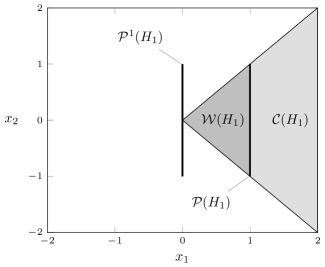
Figure 1: RNIEP & SNIEP for $n=2$.

Case $n=3$. Let

$$S:=H_{1}\oplus H_{0}=\begin{bmatrix}1&1&0\\ 1&-1&0\\ 0&0&1\end{bmatrix}~{}\mbox{and}~{}P:=\begin{bmatrix}1&0&0\\ 0&0&1\\ 0&1&0\end{bmatrix}.$$

For $a\in[0,1]$, let $b:=1-a$ and

$$S_{a}:=\begin{bmatrix}1&1&0\\ 1&-a&1\\ 1&-a&-1\end{bmatrix}.$$

Figure 2 depicts the projected Perron spectratopes for the matrices $S$, $SP$, and $S_{a}$.

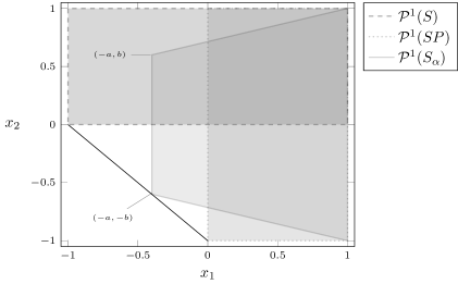
Figure 2: RNIEP & SNIEP for $n=3$.

A straightforward calculation reveals that if $v=[1~{}x~{}y]^{\top}$, then the matrix $S_{a}D_{v}S_{a}^{-1}$ is given by

$$\frac{1}{2(1+a)}\begin{bmatrix}2(x+a)&1-x&1-x\\ 2a(1-x)&a(x+y)+y+1&a(x-y)-y+1\\ 2a(1-x)&a(x-y)-y+1&a(x+y)+y+1\end{bmatrix}.$$

Furthermore, if $u=[1~{}\sqrt{2a}~{}\sqrt{2a}]^{\top}$, then the matrix $D_{u}^{-1}S_{a}D_{v}S_{a}^{-1}D_{u}$ is given by

$$\frac{1}{2(1+a)}\begin{bmatrix}2(x+a)&\sqrt{2a}(1-x)&\sqrt{2a}(1-x)\\ \sqrt{2a}(1-x)&a(x+y)+y+1&a(x-y)-y+1\\ \sqrt{2a}(1-x)&a(x-y)-y+1&a(x+y)+y+1\end{bmatrix},$$

thus, the realizing matrix can by taken to be symmetric.

Case $n=4$. Without loss of generality, assume that $\lambda_{1}\geq\lambda_{2}\geq\lambda_{3}\geq\lambda_{4}$. If $v:=[\lambda_{1}~{}\lambda_{4}~{}\lambda_{2}~{}\lambda_{3}]^{\top}$ and $S:=H_{1}\oplus H_{1}$, then

$$SD_{v}S^{-1}=\frac{1}{2}\begin{bmatrix}\lambda_{1}+\lambda_{4}&\lambda_{1}-\lambda_{4}&0&0\\ \lambda_{1}-\lambda_{4}&\lambda_{1}+\lambda_{4}&0&0\\ 0&0&\lambda_{2}+\lambda_{3}&\lambda_{2}-\lambda_{3}\\ 0&0&\lambda_{2}-\lambda_{3}&\lambda_{2}+\lambda_{3}\end{bmatrix}.$$

Thus, $\mathcal{C}\left(S\right)$ contains all spectra such that

1. $\lambda_{1}\geq\lambda_{2}\geq\lambda_{3}\geq\lambda_{4}\geq 0$;

2. $\lambda_{1}\geq\lambda_{2}\geq\lambda_{3}\geq 0>\lambda_{4}$; or

3. $\lambda_{1}\geq\lambda_{2}\geq 0>\lambda_{3}\geq\lambda_{4}$, and $\lambda_{2}+\lambda_{3}\geq 0$.

If $H_{2}:=H_{1}\otimes H_{1}$, then $H_{2}D_{v}H_{2}^{-1}$ equals

$$\frac{1}{4}\begin{bmatrix}\lambda_{1}+\lambda_{4}+\lambda_{2}+\lambda_{3}&\lambda_{1}-\lambda_{4}+\lambda_{2}-\lambda_{3}&\lambda_{1}+\lambda_{4}-\lambda_{2}-\lambda_{3}&\lambda_{1}-\lambda_{4}-\lambda_{2}+\lambda_{3}\\ \lambda_{1}-\lambda_{4}+\lambda_{2}-\lambda_{3}&\lambda_{1}+\lambda_{4}+\lambda_{2}+\lambda_{3}&\lambda_{1}-\lambda_{4}-\lambda_{2}+\lambda_{3}&\lambda_{1}+\lambda_{4}-\lambda_{2}-\lambda_{3}\\ \lambda_{1}+\lambda_{4}-\lambda_{2}-\lambda_{3}&\lambda_{1}-\lambda_{4}-\lambda_{2}+\lambda_{3}&\lambda_{1}+\lambda_{4}+\lambda_{2}+\lambda_{3}&\lambda_{1}-\lambda_{4}+\lambda_{2}-\lambda_{3}\\ \lambda_{1}-\lambda_{4}-\lambda_{2}+\lambda_{3}&\lambda_{1}+\lambda_{4}-\lambda_{2}-\lambda_{3}&\lambda_{1}-\lambda_{4}+\lambda_{2}-\lambda_{3}&\lambda_{1}+\lambda_{4}+\lambda_{2}+\lambda_{3}\end{bmatrix}.$$

Thus, $\mathcal{C}\left(S\right)$ contains all spectra such that

1. $\lambda_{1}\geq\lambda_{2}\geq 0>\lambda_{3}\geq\lambda_{4}$, and $\lambda_{2}+\lambda_{3}<0$; or

2. $\lambda_{1}\geq 0>\lambda_{2}\geq\lambda_{3}\geq\lambda_{4}$.

Figure 3 depicts the projected Perron spectratope of $H_{2}$, as established in Corollary 5.26. ∎

Figure 3: $\mathcal{P}^{1}(H_{2})$.

Figure 2 suggests that the trace-nonnegative polytope $\mathcal{T}^{2}$ can not be covered by countably many projected Perron spectratopes; this can be proven via the relative gain array.

Lemma 4.21.

Suppose that $S$ is a $3$-by-$3$ Perron-similarity. If $x$, $y\in\mathcal{C}\left(S\right)$ such that $e^{\top}x=e^{\top}y=0$, then $x=y$.

Proof.

If $x\neq y$, then $\operatorname{\rm rank}\left(\Phi(S)\right)=1$; hence

$$\Phi(S)=\begin{bmatrix}a&b&c\\ ka&kb&kc\\ \ell a&\ell b&\ell c\end{bmatrix}.$$

Since $\Phi(S)$ has row and column sums equal to one ([15, §2, Observation 1]), it follows that $k=\ell=1$, and $a=b=c=1/3$; however, as noted in [15, §5, Example 2], the equation $\Phi(X)=(1/3)J$ has no real solutions. ∎

Corollary 4.22.

If $\{S_{\alpha}\}_{\alpha\in\mathcal{I}}$ is a collection of invertible $3$-by-$3$ matrices such that

$$\bigcup_{\alpha\in\mathcal{I}}\mathcal{P}^{1}(S_{\alpha})=\mathcal{T}^{2},$$

then $\mathcal{I}$ is uncountable.

5 Perron Spectratopes of Hadamard Matrices

Recall that $H$ is a Hadamard matrix if $h_{ij}\in\{\pm 1\}$ and $HH^{\top}=nI$. If $n$ is a positive integer $n$ such that there is a Hadamard matrix of order $n$, then $n$ is called a Hadamard order. The longstanding Hadamard conjecture asserts that there is a Hadamard matrix of order $4k$ exists for every $k\in\mathbb{N}$.

Let $H_{0}=[1]$, and for $n\in\mathbb{N}$, let

$$H_{n}:=H_{1}\otimes H_{n-1}=\left[\begin{array}[]{rr}H_{n-1}&H_{n-1}\\ H_{n-1}&-H_{n-1}\end{array}\right]\in\textsl{M}_{2^{n}}(\mathbb{R}).$$ (5.3)

It is well-known that $H_{n}$ is a Hadamard matrix for every $n\in\mathbb{N}_{0}$, and the construction given in (5.3) is known as the Sylvester construction, and the matrix $H_{n}$, $n\in\mathbb{N}_{0}$ is called the canonical Hadamard, or Walsh matrix of order $2^{n}$ (for brevity, and given that Sylvester matrix is reserved for another matrix, we will use the latter term).

Walsh matrices satisfy the following additional well-known properties:

1. $H_{n}=H_{n}^{\top}$;

2. $H_{n}^{-1}=2^{-n}H_{n}$;

3. $\operatorname{\rm tr}\left(H_{n}\right)=0$, $n\geq 1$;

4. $e_{1}^{\top}H_{n}=e^{\top}$;

5. $H_{n}e_{1}=e$; and

6. $e^{\top}H_{n}=ne_{1}$.

Lastly, note that $H_{n}$ is a Perron similarity for every $n$.

Proposition 5.23.

Let

$$P_{11}:=\begin{bmatrix}1&0\\ 0&1\end{bmatrix}\mbox{ and }P_{12}:=\begin{bmatrix}0&1\\ 1&0\end{bmatrix}.$$

For $n\geq 2$, let

$$P_{nk}:=\left\{\begin{array}[]{rl}P_{11}\otimes P_{(n-1)k}=\begin{bmatrix}P_{(n-1)k}&0\\ 0&P_{(n-1)k}\end{bmatrix}\in\textsl{M}_{2^{n}}(\mathbb{R}),&k\in\langle 2^{n-1}\rangle\\ \\ P_{12}\otimes P_{(n-1)\ell}=\begin{bmatrix}0&P_{(n-1)\ell}\\ P_{(n-1)\ell}&0\end{bmatrix}\in\textsl{M}_{2^{n}}(\mathbb{R}),&k\in\langle 2^{n}\rangle\backslash\langle 2^{n-1}\rangle,\end{array}\right.$$

where $\ell=k-2^{n-1}$. Then, for $n\in\mathbb{N}$:

1. $P_{n1}=I$;

2. $P_{n2^{n}}=K$;

3. $P_{nk}$ is a trisymmetric permutation matrix, $\forall k\in\langle 2^{n}\rangle$;

4. $\sum_{k=1}^{2^{n}}P_{nk}=J$;

5. If $\mathscr{P}_{n}:=\left\{P_{n1},\dots,P_{n2^{k}}\right\}$, then $\{\mathscr{P}_{n},\times\}\cong(\mathbb{Z}_{2})^{n}$;

6. $P_{nk}^{2}=I$;

7. if $v^{\top}:=e_{k}^{\top}H_{n}$, then $P_{nk}=2^{-n}H_{n}D_{v}H_{n}$, $\forall k\in\langle 2^{n}\rangle$;

8. for every $k\neq\ell$, $\left\langle P_{nk},P_{n\ell}\right\rangle:=\operatorname{\rm tr}\left(P_{nk}^{\top}P_{n\ell}\right)=0$; and

9. for every $k$, $\ell\in\langle n\rangle$, there is a $j\in\langle n\rangle$ such that $P_{nk}P_{n\ell}=P_{n\ell}P_{nk}=P_{nj}$.

Proof.

Parts (i)–(v) follow readily by induction on $n$; part (vi) follows from part (iii); part (viii) follows from parts (iii) and (iv); and part (ix) follows from parts (v) and (vii) (alternately, part (ix) follows from part (vii) and the fact that the rows of $H_{n}$ form a group with respect to Hadamard product).

For part (vii), we proceed by induction on $n$: for $n=1$, the result follows by a direct computation.

Assume that the result holds when $n=m>1$. If $v\in\mathbb{R}^{2^{m+1}}$, and $u$ and $w$ are the vectors in $\mathbb{R}^{2^{m}}$ defined by

$$v=\begin{bmatrix}u\\ w\end{bmatrix},$$ (5.4)

then $D_{v}=D_{u}\oplus D_{w}$ and

$$H_{m+1}D_{v}H_{m+1}=\begin{bmatrix}H_{m}D_{u+w}H_{m}&H_{m}D_{u-w}H_{m}\\ H_{m}D_{u-w}H_{m}&H_{m}D_{u+w}H_{m}\end{bmatrix}.$$ (5.5)

We distinguish the following cases:

1. $k\in\langle 2^{m}\rangle$. If $v^{\top}:=e_{k}^{\top}H_{m+1}$, then, $u=w=H_{m}e_{k}$. Following (5.5) and the induction-hypothesis, notice that

   $$H_{m+1}D_{v}H_{m+1} =\begin{bmatrix}2H_{m}D_{u}H_{m}&0\\ 0&2H_{m}D_{u}H_{m}\end{bmatrix}$$

   $$=\begin{bmatrix}2\cdot 2^{m}P_{mk}&0\\ 0&2\cdot 2^{m}P_{mk}\end{bmatrix}=2^{m+1}P_{(m+1)k},$$

   and the result is established.

2. $k\in\langle 2^{m+1}\rangle\backslash\langle 2^{m}\rangle$. If $v^{\top}:=e_{k}^{\top}H_{m+1}$, then $u=-w=H_{m}e_{\ell}$, where $\ell:=k-2^{m-1}$. Following (5.5) and the induction-hypothesis, notice that

   $$H_{m+1}D_{v}H_{m+1} =\begin{bmatrix}0&2H_{m}D_{u}H_{m}\\ 2H_{m}D_{u}H_{m}&0\end{bmatrix}$$

   $$=\begin{bmatrix}0&2\cdot 2^{m}P_{m\ell}\\ 2\cdot 2^{m}P_{m\ell}&0\end{bmatrix}=2^{m+1}P_{(m+1)k},$$

   and the result is established. ∎

Theorem 5.24.

The Perron spectracone of the Walsh matrix of order $2^{n}$ is the conical hull of its rows.

Proof.

For $x\in\mathbb{C}^{2^{n}}$, let $v^{\top}:=x^{\top}H_{n}$, and $M=M_{x}:=2^{-n}H_{n}D_{v}H_{n}$. Since

$$v^{\top}=x^{\top}H_{n}=\left(\sum_{k=1}^{2^{n}}x_{k}e_{k}^{\top}\right)H_{n}=\sum_{k=1}^{2^{n}}x_{k}\left(e_{k}^{\top}H_{n}\right)=\sum_{k=1}^{2^{n}}x_{k}v_{k}^{\top},$$

where $v_{k}:=e_{k}^{\top}H_{n}$, it follows from part (vii) of Proposition 5.23 that

$$M=2^{-n}H_{n}D_{v}H_{n}=\sum_{k=1}^{2^{n}}x_{k}\left(2^{-n}H_{n}D_{v_{k}}H_{n}\right)=\sum_{k=1}^{2^{n}}x_{k}P_{nk},$$

i.e., $M\in\operatorname{\rm span}\left(\mathscr{P}_{n}\right)$.

In view of parts (iii) and (iv) of Propostion 5.23, it follows that the $k\textsuperscript{th}$-entry of $x$ appears exactly once in each row and column of $M$. Thus, $M\geq 0$ if and only if $x\geq 0$, i.e., if and only if $v\in\operatorname{\rm coni}\left(v_{1},\dots,v_{2^{n}}\right)$. ∎

The following result is useful in quickly determining whether a vector belongs to $\mathcal{C}\left(H_{n}\right)$.

Corollary 5.25.

If $v\in\mathbb{R}^{2^{n}}$, where $v_{1}\geq\cdots\geq v_{n}$, then $v\in\mathcal{C}\left(H_{n}\right)$ if and only if $H_{n}v\geq 0$.

Proof.

If $v\in\mathcal{C}\left(H_{n}\right)$, then following Theorem 5.24, there is a nonnegative vector $x$ such that $v=H_{n}x$; multipying both sides of this equation by $H_{n}$ yields $H_{n}v=2^{n}x\geq 0$.

Conversely, if $x:=H_{n}v\geq 0$, then $H_{n}x=2^{n}v$, i.e., $v=H_{n}(x/2^{n})$; the result now follows from Theorem 5.24. ∎

Parts (i), (iii), (iv), and (ix) of Propostion 5.23 demonstrate that $\mathscr{P}_{n}$ is a $(2^{n}-1)$-class symmetric (and hence commutative) association scheme (see, e.g., the survey [19] and references therein). As a consequence, $\mathcal{A}(H_{n})$ is a nonnegative Bose-Mesner algebra, i.e., it is closed with respect to matrix transposition, matrix multiplication, and Hadamard product.

A straightforward proof by induction shows that

$$M_{x}=\begin{bmatrix}x^{\top}P_{n1}\\ \vdots\\ x^{\top}P_{n2^{k}}\end{bmatrix}=\begin{bmatrix}P_{n1}x&\cdots&P_{n2^{k}}x\end{bmatrix}.$$

For example, if $x\in\mathbb{C}^{8}$, then

$$M_{x}=\left[\begin{array}[]{*{4}{c}|*{4}{c}}x_{1}&x_{2}&x_{3}&x_{4}&x_{5}&x_{6}&x_{7}&x_{8}\\ x_{2}&x_{1}&x_{4}&x_{3}&x_{6}&x_{5}&x_{8}&x_{7}\\ x_{3}&x_{4}&x_{1}&x_{2}&x_{7}&x_{8}&x_{5}&x_{6}\\ x_{4}&x_{3}&x_{2}&x_{1}&x_{8}&x_{7}&x_{6}&x_{5}\\ \hline\cr x_{5}&x_{6}&x_{7}&x_{8}&x_{1}&x_{2}&x_{3}&x_{4}\\ x_{6}&x_{5}&x_{8}&x_{7}&x_{2}&x_{1}&x_{4}&x_{3}\\ x_{7}&x_{8}&x_{5}&x_{6}&x_{3}&x_{4}&x_{1}&x_{2}\\ x_{8}&x_{7}&x_{6}&x_{5}&x_{4}&x_{3}&x_{2}&x_{1}\end{array}\right].$$

Moreover, if $x$, $y\in\mathbb{C}$, then $M_{x}\circ M_{y}=M_{x\circ y}$ and $M_{x}M_{y}=M_{z}$, where

$$z=\begin{bmatrix}x^{\top}P_{n1}y\\ x^{\top}P_{n2}y\\ \vdots\\ x^{\top}P_{n2^{k}}y\end{bmatrix}=\begin{bmatrix}x^{\top}y\\ x^{\top}P_{n2}y\\ \vdots\\ x^{\top}Ky\end{bmatrix}.$$

Corollary 5.26.

The Perron spectratope of the Walsh matrix of order $2^{n}$ is the convex hull of its rows.

The import of Corollary 5.26 can be viewed through the following lens: given an affinely independent set $V=\{v_{1},\dots,v_{n+1}\}\in\mathbb{R}^{n}$, recall that the n-simplex of $V$ is the set $\mathcal{S}(V):=\operatorname{\rm conv}\left(V\right)$. It is well-known (see, e.g., [26]) that

$$\operatorname{Vol}\left(\mathcal{S}(V)\right)=\left|\frac{1}{n!}\det{M}\right|,$$ (5.6)

where

$$M=\begin{bmatrix}1&v_{1}^{\top}\\ \vdots&\vdots\\ 1&v_{n+1}^{\top}\end{bmatrix}.$$

Thus,

$$\operatorname{Vol}\left(\mathcal{W}(H_{n})\right)=\frac{1}{(2^{n})!}2^{n2^{n-1}}~{}\mbox{and}~{}\operatorname{Vol}\left(\mathcal{P}^{1}(H_{n})\right)=\frac{1}{(2^{n}-1)!}2^{n2^{n-1}}.$$

We call a nonsingular matrix $S$ a strong Perron similarity if there is a unique $i\in\langle n\rangle$ such that $Se_{i}>0$ and $e_{i}^{\top}S^{-1}>0$. If $S\in GL_{n}(\mathbb{R})$ is a strong Perron similarity, then, without loss of generality, $S=[e~{}s_{2}~{}\cdots~{}s_{n}]$, where $||s_{i}||_{\infty}=1$.

Since a Hadamard matrix has maximal determinant among matrices whose entries are less than or equal to 1 in absolute value, it follows that if $\mathcal{P}^{1}(S)=\mathcal{S}(s_{2},\dots,s_{2^{n}})$, then $\operatorname{Vol}\left(\mathcal{P}^{1}(S)\right)\leq\operatorname{Vol}\left(\mathcal{P}^{1}(H_{n})\right)$. It is an open question whether $\mathcal{P}^{1}(H_{n})$ has maximal volume for all Perron spectratopes.

Moreover, Corollary 5.26 does not seem to hold for general Hadamard matrices. If $H$ is a Hadamard matrix, then any matrix resulting from negating its rows or columns is also a Hadamard matrix. Indeed, if $u$ denotes the $i\textsuperscript{th}$-column of $H$ and $w$ denotes its $i\textsuperscript{th}$-row, then the $i\textsuperscript{th}$-row and $i\textsuperscript{th}$-column of the Hadamard matrix $\hat{H}=D_{h_{ii}u}HD_{w}$ are positive. Thus, without loss of generaltiy, we assume that the first row and column of any Hadamard matrix are positive and refer to such a matrix as a normalized Hadamard matrix.

It can be verified via the MATLAB-command Hadamard(12) that only the first row of the normalized Hadamard matrix of order twelve belongs to its Perron spectratope. However, it is clear every row of a normalized Hadamard matrix is realizable since every row (sans the first) contains an equal number of positive and negative entries and thus is realizable (after a permutation) by the Perron similarity $\bigoplus_{i=1}^{n/2}H_{1}$.

6 Suleĭmanova spectra, the DS-RNIEP, and the DS-SNIEP

We begin with the following definition.

Definition 6.27.

We call $\sigma=\{\lambda_{1},\dots,\lambda_{n}\}\subset\mathbb{R}$ a Suleĭmanova spectrum if $s_{1}(\sigma)\geq 0$ and $\sigma$ contains exactly one positive value.

In [27], Suleĭmanova stated that every such spectrum is realizable (for a proof via companion matrices, and references to other proofs, see Friedland [10]). Fiedler [9] proved that every Suleĭmanova spectrum is symmetrically realizable. In [14], Johnson et al. posed the following.

Problem 6.28.

If $\sigma$ is a normalized Suleĭmanova spectrum, is $\sigma$ realizable by a doubly stochastic matrix?

We will show that for Hadamard orders, the answer is ‘yes’ and the realizing matrix can be taken to be symmetric.

Theorem 6.29.

If $H$ is a normalized Hadamard matrix of order $n$ and $\sigma=\{\lambda_{1},\dots,\lambda_{n}\}$ is a normalized Suleĭmanova spectrum, then $\sigma$ is realizable by a symmetric, doubly stochastic matrix.

Proof.

It suffices to show that $v:=[1~{}\cdots~{}\lambda_{n}]^{\top}\in\mathcal{P}\left(H\right)$. For $k\in\langle n\rangle$, $k\neq 1$, let $D_{k}:=e_{1}e_{1}^{\top}-e_{k}e_{k}^{\top}$ and $M_{k}:=n^{-1}HD_{k}H^{\top}$. Then

$$nM_{k} =H\left(e_{1}e_{1}^{\top}-e_{k}e_{k}^{\top}\right)H^{\top}$$

$$=He_{1}\left(He_{1}\right)^{\top}-He_{k}\left(He_{k}\right)^{\top}=J-He_{k}\left(He_{k}\right)^{\top}.$$

Because the matrix $He_{k}\left(He_{k}\right)^{\top}$ has entries in $\{\pm 1\}$, the matrix $J-He_{k}\left(He_{k}\right)^{\top}$ has entries in $\{0,2\}$, i.e., $M_{k}\geq 0$. Moreover, $\operatorname{\rm Diag}\left(D_{k}\right)=e_{1}-e_{k}$ so that $e_{1}-e_{k}\in\mathcal{P}\left(H\right)$.

Since $\mathcal{P}\left(H\right)$ is convex and $\{e_{1},e_{1}-e_{2},\dots,e_{1}-e_{n}\}\subset\mathcal{P}\left(H\right)$, it follows that $\operatorname{\rm conv}\left(e_{1},e_{1}-e_{2},\dots,e_{1}-e_{n}\right)\subseteq\mathcal{P}\left(H\right)$. If $\mu_{1}:=s_{1}(\sigma)$ and $\mu_{k}:=-\lambda_{k}$, for $k\geq 2$, then $\mu_{k}\geq 0$, $\sum_{k=1}^{n}\mu_{k}=1$, and

$$v =e_{1}+\sum_{k=2}^{n}\lambda_{k}e_{k}$$

$$=e_{1}+\sum_{k=2}^{n}(\lambda_{k}+\mu_{k})e_{1}+\sum_{k=2}^{n}\lambda_{k}e_{k}$$

$$=\mu_{1}e_{1}+\sum_{k=2}^{n}\mu_{i}(e_{1}-e_{k}).$$

Thus, $v\in\operatorname{\rm conv}\left(e_{1},e_{1}-e_{2},\dots,e_{1}-e_{n}\right)$ and the result is established. ∎

Remark 6.30.

For any normalized Hadamard matrix, notice that

$$\mathcal{H}_{n}:=\operatorname{\rm conv}\left(e,e_{1}-e_{2},\dots,e_{1}-e_{n}\right)\subseteq\mathcal{P}\left(H\right).$$

Since

$$\frac{1}{n}\left[e+\sum_{k=2}^{n}(e_{1}-e_{k})\right]=e_{1},$$

it follows that

$$\operatorname{\rm conv}\left(e_{1},e_{1}-e_{2},\dots,e_{1}-e_{n}\right)\subset\mathcal{H}_{n}\subseteq\mathcal{P}\left(H\right).$$

Thus,

$$\bigcap_{\mathscr{H}_{n}}\mathcal{P}\left(H\right)=\mathcal{H}_{n},$$

where $\mathscr{H}_{n}$ contains every normalized Hadamard matrix of order $n$.

In terms of the projected Perron spectratope, notice that

$$\pi_{1}(\mathcal{H}_{n})=\operatorname{\rm conv}\left(e,-e_{2},\dots,-e_{n}\right)\subseteq\mathcal{P}^{1}(H)\subset\mathcal{T}^{n-1}$$

If

$$S=\begin{bmatrix}1&e^{\top}\\ e&-I\end{bmatrix}\in GL_{n}(\mathbb{R}),~{}n\geq 2$$

then $\det{S}=(-1)^{n+1}n$. Following (5.6),

$$\operatorname{Vol}\left(\mathcal{P}^{1}(H)\right)\geq\operatorname{Vol}\left(\pi_{1}(\mathcal{H}_{n})\right)=\frac{n}{(n-1)!}=\frac{n^{2}}{n!}.$$

The following result is corollary to Corollary 5.26 and Theorem 6.29.

Corollary 6.31.

If $\sigma=\{\lambda_{1},\dots,\lambda_{2^{n}}\}$ is a normalized Suleĭmanova spectrum, then $\sigma$ is realizable by a trisymmetric doubly stochastic matrix.

In [9], Fiedler showed that every Suleĭmanova spectrum is symmetrically realizable. However, his proof is by induction and therefore does not explicitly yield a realizing matrix (the computation of which is of interest for numerical purposes), which is common for many NIEP results. Indeed, according to Chu: Very few of these theoretical results are ready for implementation to actually compute [the realizing] matrix. The most constructive result we have seen is the sufficient condition studied by Soules [25]. But the condition there is still limited because the construction depends on the specification of the Perron vector – in particular, the components of the Perron eigenvector need to satisfy certain inequalities in order for the construction to work. [3, p. 18]. Thus, Theorem 6.29 and Corollary 6.31 are constructive versions of Fiedler’s result for Hadamard powers.

Corollary 6.32.

If $\sigma=\{\lambda_{1},\dots,\lambda_{n}\}$ is a normalized Suleĭmanova spectrum, then there is a nonnegative integer $N$ such that

$$\hat{\sigma}:=\sigma\cup\{\overbrace{0,\dots,0}^{N}\}$$

is realized by a symmetric, doubly stochastic $(n+N)$-by-$(n+N)$ matrix. If $n+N$ is a power of two, then the realizing matrix is trisymmetric.

Remark 6.33.

If the Hadamard conjecture holds, then $N\leq 3$. Moreover, Corollary 6.32 is a constructive version of the celebrated Boyle-Handelman theorem [2, Theorem 5.1] for Suleĭmanova spectra.

A natural variation of Problem 6.28 is the following.

Problem 6.34.

If $\sigma=\{\lambda_{1},\dots,\lambda_{n}\}$, $n\geq 2$ is a normalized Suleĭmanova spectrum such that $s_{1}(\sigma)=0$, is $\sigma$ realizable by a doubly stochastic matrix?

Although the trace-zero assumption is rather restrictive, we demonstrate it is a nontrivial problem: If $A$ is a $3$-by-$3$ doubly stochastic matrix and $\operatorname{\rm tr}\left(A\right)=0$, then

$$A=\begin{bmatrix}0&a&1-a\\ 1-a&0&a\\ a&1-a&0\end{bmatrix},~{}a\in[0,1],$$

and $\sigma\left(A\right)=\{1,-1/2\pm\sqrt{3}(a-1/2)\textup{i}\}$, where $\textup{i}:=\sqrt{-1}$. Clearly, $\sigma$ is real if and only if $a=1/2$. Thus, $\{1,-1/2,-1/2\}$ is the only normalized Suleĭmanova spectrum that is realizable by a $3$-by-$3$ trace-zero doubly stochastic matrix.

We conclude with the observation that the Perron spectratopes of $H_{1}$ and $H_{2}$ resolves Problem 6.34 when $n=2$ and $n=4$, respectively (see Figure 1 and Figure 3).

References

- [1] A. Berman and R. J. Plemmons. Nonnegative matrices in the mathematical sciences, volume 9 of Classics in Applied Mathematics. Society for Industrial and Applied Mathematics (SIAM), Philadelphia, PA, 1994. Revised reprint of the 1979 original.
- [2] M. Boyle and D. Handelman. The spectra of nonnegative matrices via symbolic dynamics. Ann. of Math. (2), 133(2):249–316, 1991.
- [3] M. T. Chu. Inverse eigenvalue problems. SIAM Rev., 40(1):1–39, 1998.
- [4] G. Dahl. Combinatorial properties of Fourier-Motzkin elimination. Electron. J. Linear Algebra, 16:334–346, 2007.
- [5] P. D. Egleston, T. D. Lenker, and S. K. Narayan. The nonnegative inverse eigenvalue problem. Linear Algebra Appl., 379:475–490, 2004. Tenth Conference of the International Linear Algebra Society.
- [6] L. Elsner, R. Nabben, and M. Neumann. Orthogonal bases that lead to symmetric nonnegative matrices. Linear Algebra Appl., 271:323–343, 1998.
- [7] S. D. Eubanks. On the construction of nonnegative symmetric and normal matrices with prescribed spectral data. ProQuest LLC, Ann Arbor, MI, 2009. Thesis (Ph.D.)–Washington State University.
- [8] S. D. Eubanks and J. J. McDonald. On a generalization of Soules bases. SIAM J. Matrix Anal. Appl., 31(3):1227–1234, 2009.
- [9] M. Fiedler. Eigenvalues of nonnegative symmetric matrices. Linear Algebra and Appl., 9:119–142, 1974.
- [10] S. Friedland. On an inverse problem for nonnegative and eventually nonnegative matrices. Israel J. Math., 29(1):43–60, 1978.
- [11] R. A. Horn and C. R. Johnson. Matrix analysis. Cambridge University Press, Cambridge, 1990. Corrected reprint of the 1985 original.
- [12] C. R. Johnson. Row stochastic matrices similar to doubly stochastic matrices. Linear and Multilinear Algebra, 10(2):113–130, 1981.
- [13] C. R. Johnson, T. J. Laffey, and R. Loewy. The real and the symmetric nonnegative inverse eigenvalue problems are different. Proc. Amer. Math. Soc., 124(12):3647–3651, 1996.
- [14] C. R. Johnson, C. Marijuán, and M. Pisonero. Personal communication. 2015.
- [15] C. R. Johnson and H. M. Shapiro. Mathematical aspects of the relative gain array . SIAM J. Algebraic Discrete Methods, 7(4):627–644, 1986.
- [16] C. Knudsen and J. J. McDonald. A note on the convexity of the realizable set of eigenvalues for nonnegative symmetric matrices. Electron. J. Linear Algebra, 8:110–114, 2001.
- [17] R. Loewy and D. London. A note on an inverse problem for nonnegative matrices. Linear and Multilinear Algebra, 6(1):83–90, 1978/79.
- [18] C. Marijuán, M. Pisonero, and R. L. Soto. A map of sufficient conditions for the real nonnegative inverse eigenvalue problem. Linear Algebra Appl., 426(2-3):690–705, 2007.
- [19] W. J. Martin and H. Tanaka. Commutative association schemes. European J. Combin., 30(6):1497–1525, 2009.
- [20] H. Minc. Nonnegative matrices. Wiley-Interscience Series in Discrete Mathematics and Optimization. John Wiley & Sons, Inc., New York, 1988. A Wiley-Interscience Publication.
- [21] H. Perfect. On positive stochastic matrices with real characteristic roots. Proc. Cambridge Philos. Soc., 48:271–276, 1952.
- [22] H. Perfect. Methods of constructing certain stochastic matrices. Duke Math. J., 20:395–404, 1953.
- [23] H. Perfect. Methods of constructing certain stochastic matrices. II. Duke Math. J., 22:305–311, 1955.
- [24] R. J. Plemmons. -matrix characterizations. I. Nonsingular -matrices. Linear Algebra and Appl., 18(2):175–188, 1977.
- [25] G. W. Soules. Constructing symmetric nonnegative matrices. Linear and Multilinear Algebra, 13(3):241–251, 1983.
- [26] P. Stein. Classroom Notes: A Note on the Volume of a Simplex. Amer. Math. Monthly, 73(3):299–301, 1966.
- [27] H. R. Suleĭmanova. Stochastic matrices with real characteristic numbers. Doklady Akad. Nauk SSSR (N.S.), 66:343–345, 1949.