NONLINEAR THREE POINT SINGULAR BVPs : A CLASSIFICATION

Abstract

We analyze the existence of unique solutions of the following class of nonlinear three point singular boundary value problems (SBVPs),

$$-(x^{\alpha}y^{\prime}(x))^{\prime}=x^{\alpha}f(x,y),\quad 0<x<1,$$

$$y^{\prime}(0)=0,\quad y(1)=\delta y(\eta),$$

where $\delta>0$, $0<\eta<1$ and $\alpha\geq 1$. This study shows some novel observations regarding the nature of the solution of the nonlinear three point SBVPs. We observe that when $sup\left(\partial f/\partial y\right)>0$ for $\alpha\in\cup_{n\in\mathbb{N}}\left(4n-1,4n+1\right)$ or $\alpha\in\{1,5,9,\cdots\}$ reverse ordered case occur. When $sup\left(\partial f/\partial y\right)>0$ for $\alpha\in\cup_{n\in\mathbb{N}}\left(4n-3,4n-1\right)$ or $\alpha\in\{3,7,11,\cdots\}$ and when $sup\left(\partial f/\partial y\right)<0$ for all $\alpha\geq 1$ well order case occur.

Keywords: Singular differential equation; Monotone iterative technique; Upper and lower Solutions; Reverse order; Green’s Function; Bessel function.

AMS Subject Classification: 34B16; 34B27; 34B60

1 Introduction

Nonlinear singular boundary value problems, commonly arises due to physical symmetry. Specifically, if a physical law is expressed by a Dirichlet problem $\bigtriangleup y(P)=f(P,y(P)),$ and one is interested in planar, cylindrical or spherical geometries, then it is led to the differential equation

$$-y^{\prime\prime}-\frac{\alpha}{x}y^{\prime}=f(x,y),\quad 0<x<1,$$ (1)

where $\alpha=0,1,2$, respectively [1]. In modern science various real life problems have been converted into a mathematical model similar to (1), where $\alpha\geq 0$, and several researchers have studied existence and uniqueness of the solution of (1), e.g., (see [1, 2, 3, 4, 5, 6]).

If the condition at the end point $(x=1)$ depends on some interior point of the interval $(0,1)$, then the following three point nonlinear SBVP arises

$$-(x^{\alpha}y^{\prime}(x))^{\prime}=x^{\alpha}f(x,y),\quad 0<x<1,$$ (2)

$$y^{\prime}(0)=0,\quad y(1)=\delta y(\eta),$$ (3)

where $f:I\times R\rightarrow R,~{}I=[0,1],~{}0<\eta<1,~{}\delta>0$ and $\alpha\geq 1$. Different analytical techniques are available for solvability of three point nonlinear BVPs, for $\alpha=0,1$ and $2$ (see [7, 8, 9, 10, 11, 12, 13]. The results of this paper may lead to some new developments in this area.

Two point BVPs are studied extensively when upper and lower solutions are well ordered. But when upper and lower solutions are in the reversed order (see [13, 14, 15, 16, 17, 18] and the reference there in) lot of explorations are still left unattended for both two point and multi point boundary value problems. In this paper we have tried to analyze few of these gaps related to monotone iterative techniques.

If $f(x,y)$ is continuous and Lipschitz continuous in its domain, we derive the following monotone iterative scheme from the nonlinear singular three point BVP (2)–(3),

$$-y_{n+1}^{\prime\prime}(x)-\frac{\alpha}{x}y_{n+1}^{\prime}(x)-\lambda y_{n+1}(x)=f(x,y_{n})-\lambda y_{n}(x),\quad y_{n+1}^{\prime}(0)=0,\quad y_{n+1}(1)=\delta y_{n+1}(\eta),$$ (4)

and prove that solution exists and belongs to the class $C[0,1]\cap~{}C^{2}[0,1]$.

We also define upper and lower solution which are our initial guesses for the above iterative scheme.

Definition 1.1

If the functions $u_{0},v_{0}\in C^{2}[0,1]$ are defined as

$$-(x^{\alpha}u_{0}^{\prime}(x))^{\prime}\geq x^{\alpha}f(x,u_{0}),\quad 0<x<1;$$ (5)

$$~{}~{}u_{0}^{\prime}(0)=0,\quad u_{0}(1)\geq\delta u_{0}(\eta),$$ (6)

$$-(x^{\alpha}v_{0}^{\prime}(x))^{\prime}\leq x^{\alpha}f(x,v_{0}),\quad 0<x<1;$$ (7)

$$~{}~{}v_{0}^{\prime}(0)=0,\quad v_{0}(1)\leq\delta v_{0}(\eta),$$ (8)

then $u_{0}$ and $v_{0}$ are called upper and lower solutions of the nonlinear three point SBVPs (2)–(3), respectively.

The purpose of this paper is to prove existence of unique solution for the class of nonlinear three point SBVPs. We observe that depending on the values of $\alpha$ we arrive at well ordered and reversed order cases. This classification, we deduce does not exist in the literature to the best of our knowledge.

This paper is organized in the following sections. Section 2 we use Lommel’s transformation to find out two linearly independent solutions in the terms of Bessel functions. Using these two linearly independent solutions Green’s functions are constructed for different class of $\alpha$ (See Figure 1) in Section 3 and Section 4 states maximum and anti-maximum principles. Finally in Section 5 all these results are used to establish some new existence and uniqueness theorems. The sufficient conditions derived in this paper are verified for certain values which belongs to different classes of $\alpha$ in Section 6.

2 The Linear Case

The linear BVP corresponding to the nonlinear three point SBVPs (2)–(3) is studied in this section. We consider the following inhomogeneous class of three point linear SBVPs,

$$-(x^{\alpha}y^{\prime}(x))^{\prime}-\lambda x^{\alpha}y(x)=x^{\alpha}h(x),\quad 0<x<1,$$ (9)

$$y^{\prime}(0)=0,\quad y(1)=\delta y(\eta)+b,$$ (10)

where $h\in C(I)$ and $b$ is any constant. To solve the inhomogeneous system (9)–(10), we consider the corresponding homogeneous system

$$-(x^{\alpha}y^{\prime}(x))^{\prime}-\lambda x^{\alpha}y(x)=0,\quad 0<x<1,$$ (11)

$$y^{\prime}(0)=0,\quad y(1)=\delta y(\eta).$$ (12)

Using Lommel’s transformation (§cf [5, 19]) $z=\beta\zeta^{\gamma}$, $w=\zeta^{-a}v(\zeta)$, the standard Bessel’s equation (13) is transformed into (14)

$$z^{2}\frac{d^{2}w}{dz^{2}}+z\frac{dw}{dz}+(z^{2}-\nu^{2})w=0,$$ (13)

$${\zeta}^{2}\frac{d^{2}v}{d{\zeta}^{2}}+{\zeta}(1-2a)\frac{dv}{d{\zeta}}+\left[(\beta\gamma\zeta^{\gamma})^{2}+(a^{2}-\nu^{2}\gamma^{2})\right]v=0.$$ (14)

Now, by Lommel’s Transformation the two linearly independent solutions of (14) are given by

$$v_{1}(x)=\zeta^{a}w_{1}\left(\beta\zeta^{\gamma}\right),\quad v_{2}(x)=\zeta^{a}w_{2}\left(\beta\zeta^{\gamma}\right),$$ (15)

where $w_{1}(z)$ and $w_{2}(z)$ are two linearly independent solutions of Bessel’s equation (13).
Now, if we set $\nu=a=\frac{1-\alpha}{2}$, $\gamma=1$, $\beta^{2}=\lambda$, then (14) reduces to (11) and hence we can obtained the two linearly independent solutions of (11) in terms of $w_{1}(z)$ and $w_{2}(z)$. A solution of (11) which is bounded in the neighborhood of the origin (except for a multiplicative constant) given by $x^{\nu}J_{-\nu}\left(x\sqrt{\lambda}\right),~{}\mbox{if $\lambda>0$}~{}\mathrm{and}~{}x^{\nu}I_{-\nu}\left(x\sqrt{|\lambda|}\right),~{}\mbox{if $\lambda<0$}$.

Note 2.1

In this paper $J_{-\nu}$, $Y_{\nu}$ are Bessel functions of first and second kind and $I_{-\nu}$ and $K_{\nu}$ are Modified Bessel functions of first and second kind.

3 Green’s function

On the basis of sign of $\lambda$ and values of $\alpha$, we divide into the following cases.

3.0.1 Case I: When $\lambda>0$ and $\alpha\notin\{1,3,5,\cdots\infty\}$.

Suppose that

• $0<\lambda<j^{2}_{\nu,1}$,  $0<\delta<1$,  $\delta\eta^{\nu}J_{\nu}\left(\eta\sqrt{\lambda}\right)-J_{\nu}\left(\sqrt{\lambda}\right)\geq 0$ and $J_{-\nu}\left(\sqrt{\lambda}\right)-\delta\eta^{\nu}J_{-\nu}\left(\eta\sqrt{\lambda}\right)>0$,
  for $\alpha\in\bigcup_{n\in N}(4n-3,4n-1)$, and

• $0<\lambda<j^{2}_{\nu,1}$,  $\delta\geq 1$,  $\delta\eta^{\nu}J_{\nu}\left(\eta\sqrt{\lambda}\right)-J_{\nu}\left(\sqrt{\lambda}\right)\leq 0$ and $J_{-\nu}\left(\sqrt{\lambda}\right)-\delta\eta^{\nu}J_{-\nu}\left(\eta\sqrt{\lambda}\right)<0$,
  for $\alpha\in\bigcup_{n\in N}(4n-1,4n+1)$,

where $j^{2}_{\nu,1}$ is the first zero of $J_{\nu}(x)$. We can easily check the validation of $(H_{0})$ and $(H_{1})$ for $\alpha\in\bigcup_{n\in N}(4n-3,4n-1)$ and $\alpha\in\bigcup_{n\in N}(4n-1,4n+1)$ respectively.

Next two lemmas help us to define the sign of Green’s function.

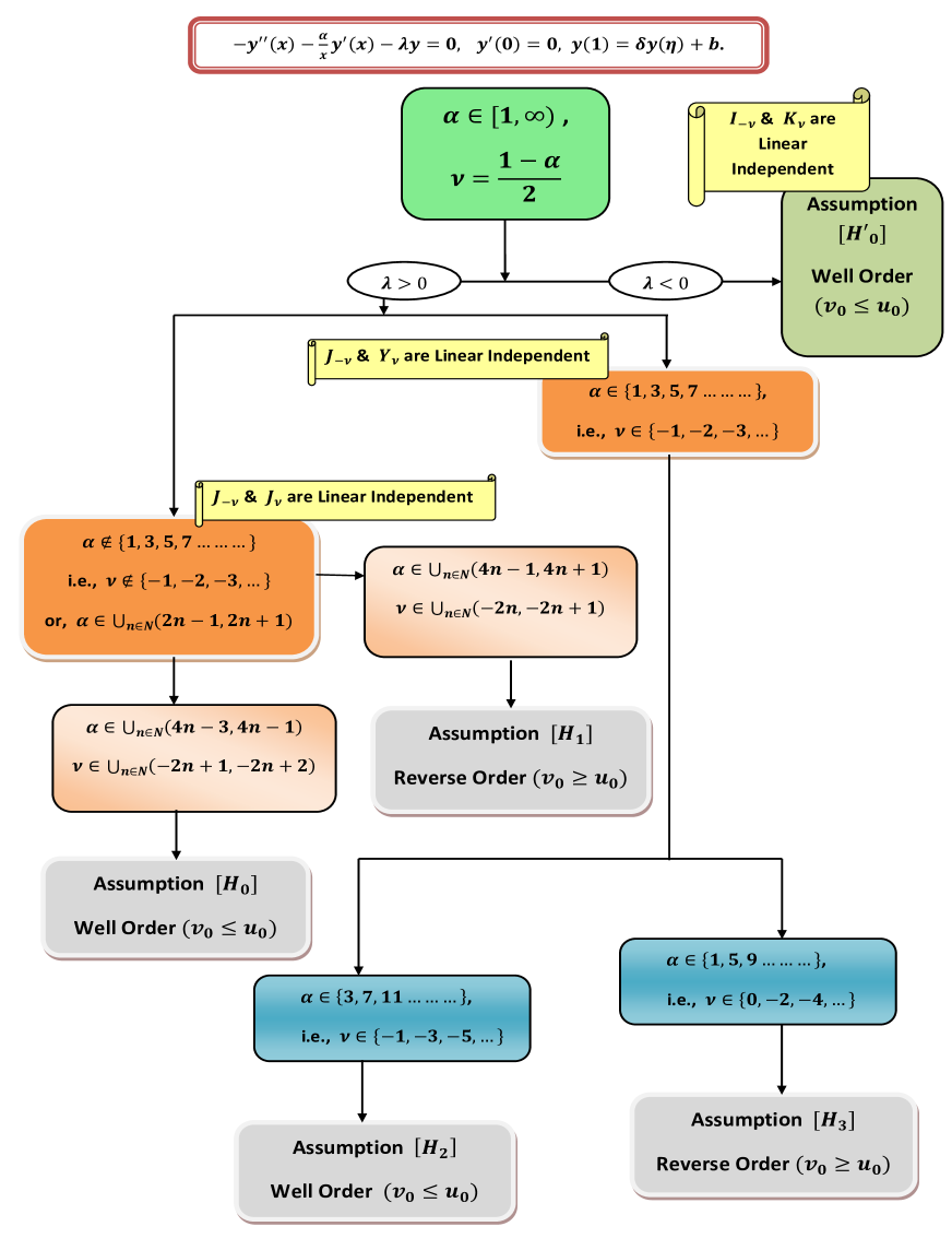
Figure 1: Flow Chart

Lemma 3.1

For $0<\lambda<\ j_{\nu,1}^{2}$, the Bessel functions of first kind $(J_{\nu}$ and $J_{-\nu})$ satisfy the following inequality

$$r^{\nu}\left(J_{-\nu}\left(s\sqrt{\lambda}\right)J_{\nu}\left(r\sqrt{\lambda}\right)-J_{\nu}\left(s\sqrt{\lambda}\right)J_{-\nu}\left(r\sqrt{\lambda}\right)\right)\geq 0,~{}~{}0<r\leq s\leq 1,$$

where $\nu=\frac{1-\alpha}{2}$ and $\alpha\in\bigcup_{n\in N}(4n-3,4n-1)$.

Proof. Suppose

$$\widetilde{\Phi}(s,r)=r^{\nu}\left(J_{-\nu}\left(s\sqrt{\lambda}\right)J_{\nu}\left(r\sqrt{\lambda}\right)-J_{\nu}\left(s\sqrt{\lambda}\right)J_{-\nu}\left(r\sqrt{\lambda}\right)\right),$$

and let $s=s_{0}\in[0,1]$ be fixed. As

$$J_{-\nu}\left(s_{0}\sqrt{\lambda}\right)J_{-1+\nu}\left(r\sqrt{\lambda}\right)+J_{\nu}\left(s_{0}\sqrt{\lambda}\right)J_{1-\nu}\left(r\sqrt{\lambda}\right) \leq J_{-\nu}\left(s_{0}\sqrt{\lambda}\right)J_{-1+\nu}\left(s_{0}\sqrt{\lambda}\right)+J_{\nu}\left(s_{0}\sqrt{\lambda}\right)J_{1-\nu}\left(x_{0}\sqrt{\lambda}\right)$$

$$= \frac{2\sin{\nu\pi}}{\pi s_{0}\sqrt{\lambda}}\leq 0,$$

for $r\leq s_{0}$. Now making use of the above inequalitiy, we can easily show that $\widetilde{\Phi}(s_{0},t)$ is a non-increasing function of $r$. As $\widetilde{\Phi}(s_{0},s_{0})=0$ at $r=s_{0}$, which implies that $\widetilde{\Phi}(s_{0},r)\geq 0,~{}~{}~{}\forall~{}~{}r\leq s_{0}$. But as $s_{0}$ may have any value in $[0,1]$ therefore $\widetilde{\Phi}(s,r)\geq 0,~{}~{}\forall~{}~{}0<r\leq s\leq 1$.

Lemma 3.2

For $0<\lambda<\ j_{\nu,1}^{2}$, the Bessel functions of first kind $(J_{\nu}$ and $J_{-\nu})$ satisfy the following inequality

$$r^{\nu}\left(J_{-\nu}\left(s\sqrt{\lambda}\right)J_{\nu}\left(r\sqrt{\lambda}\right)-J_{\nu}\left(s\sqrt{\lambda}\right)J_{-\nu}\left(r\sqrt{\lambda}\right)\right)\leq 0,~{}~{}0<r\leq s\leq 1,$$

where $\nu=\frac{1-\alpha}{2}$ and $\alpha\in\bigcup_{n\in N}(4n-1,4n+1)$.

Proof. Proof follows the same analysis as we do in Lemma 3.1, with the Bessel functions inequality

$$J_{-\nu}\left(s_{0}\sqrt{\lambda}\right)J_{-1+\nu}\left(r\sqrt{\lambda}\right)+J_{\nu}\left(s_{0}\sqrt{\lambda}\right)J_{1-\nu}\left(r\sqrt{\lambda}\right) \geq J_{-\nu}\left(s_{0}\sqrt{\lambda}\right)J_{-1+\nu}\left(s_{0}\sqrt{\lambda}\right)+J_{\nu}\left(s_{0}\sqrt{\lambda}\right)J_{1-\nu}\left(s_{0}\sqrt{\lambda}\right)$$

$$= \frac{2\sin{\nu\pi}}{\pi s_{0}\sqrt{\lambda}}\geq 0,$$

for $r\leq s_{0}$.

Lemma 3.3

For the linear three point SBVPs (11)–(12), where $\alpha\notin\{1,3,5,\cdots\infty\}$, the Green’s function is given by

$$G(x,t)=\left\{\begin{array}[]{ll}\frac{\pi\csc(\pi\nu)t^{\nu}x^{\nu}J_{-\nu}\left(x\sqrt{\lambda}\right)\left(\delta\eta^{\nu}\left(J_{\nu}\left(\eta\sqrt{\lambda}\right)J_{-\nu}\left(t\sqrt{\lambda}\right)-J_{-\nu}\left(\eta\sqrt{\lambda}\right)J_{\nu}\left(t\sqrt{\lambda}\right)\right)+\left(J_{-\nu}\left(\sqrt{\lambda}\right)J_{\nu}\left(t\sqrt{\lambda}\right)-J_{\nu}\left(\sqrt{\lambda}\right)J_{-\nu}\left(t\sqrt{\lambda}\right)\right)\right)}{2\left(J_{-\nu}\left(\sqrt{\lambda}\right)-\delta\eta^{\nu}J_{-\nu}\left(\eta\sqrt{\lambda}\right)\right)},&0\leq x\leq t\leq\eta;\\ \frac{1}{2}\pi\csc(\pi\nu)t^{\nu}x^{\nu}J_{-\nu}\left(t\sqrt{\lambda}\right)\left(\frac{J_{-\nu}\left(x\sqrt{\lambda}\right)\left(\delta\eta^{\nu}J_{\nu}\left(\eta\sqrt{\lambda}\right)-J_{\nu}\left(\sqrt{\lambda}\right)\right)}{J_{-\nu}\left(\sqrt{\lambda}\right)-\delta\eta^{\nu}J_{-\nu}\left(\eta\sqrt{\lambda}\right)}+J_{\nu}\left(x\sqrt{\lambda}\right)\right),&t\leq x,~{}t\leq\eta;\\ \frac{\pi\csc(\pi\nu)t^{\nu}x^{\nu}\left(J_{-\nu}\left(\sqrt{\lambda}\right)J_{\nu}\left(t\sqrt{\lambda}\right)-J_{\nu}\left(\sqrt{\lambda}\right)J_{-\nu}\left(t\sqrt{\lambda}\right)\right)J_{-\nu}\left(x\sqrt{\lambda}\right)}{2\left(J_{-\nu}\left(\sqrt{\lambda}\right)-\delta\eta^{\nu}J_{-\nu}\left(\eta\sqrt{\lambda}\right)\right)},&x\leq t,~{}\eta\leq t;\\ \frac{1}{2}\pi\csc(\pi\nu)t^{\nu}x^{\nu}\left(\frac{J_{-\nu}\left(x\sqrt{\lambda}\right)\left(\delta\eta^{\nu}J_{-\nu}\left(\eta\sqrt{\lambda}\right)J_{\nu}\left(t\sqrt{\lambda}\right)-J_{\nu}\left(\sqrt{\lambda}\right)J_{-\nu}\left(t\sqrt{\lambda}\right)\right)}{J_{-\nu}\left(\sqrt{\lambda}\right)-\delta\eta^{\nu}J_{-\nu}\left(\eta\sqrt{\lambda}\right)}+J_{-\nu}\left(t\sqrt{\lambda}\right)J_{\nu}\left(x\sqrt{\lambda}\right)\right),&\eta\leq t\leq x\leq 1.\end{array}\right.$$

If $H_{0}$ (or $H_{1}$) holds then $G(x,t)\leq 0$ (or $G(x,t)\geq 0$).

Proof. We define Green’s function as

$$G(x,t)=\left\{\begin{array}[]{ll}a_{1}~{}x^{\nu}J_{-\nu}\left(x\sqrt{\lambda}\right)+a_{2}~{}x^{\nu}J_{\nu}\left(x\sqrt{\lambda}\right),&{0\leq x\leq t\leq\eta;}\\ a_{3}~{}x^{\nu}J_{-\nu}\left(x\sqrt{\lambda}\right)+a_{4}~{}x^{\nu}J_{\nu}\left(x\sqrt{\lambda}\right),&{t\leq x,~{}t\leq\eta;}\\ a_{5}~{}x^{\nu}J_{-\nu}\left(x\sqrt{\lambda}\right)+a_{6}~{}x^{\nu}J_{\nu}\left(x\sqrt{\lambda}\right),&{x\leq t,~{}\eta\leq t;}\\ a_{7}~{}x^{\nu}J_{-\nu}\left(x\sqrt{\lambda}\right)+a_{8}~{}x^{\nu}J_{\nu}\left(x\sqrt{\lambda}\right),&{\eta\leq t\leq x\leq 1}.\end{array}\right.$$

Using the following properties of the Green’s function, for any $t\in[0,\eta]$ and boundary conditions, we have

$$a_{1}t^{\nu}J_{-\nu}\left(t\sqrt{\lambda}\right)+a_{2}t^{\nu}J_{\nu}\left(t\sqrt{\lambda}\right)=a_{3}t^{\nu}J_{-\nu}\left(t\sqrt{\lambda}\right)+a_{4}t^{\nu}J_{\nu}\left(t\sqrt{\lambda}\right),$$

$$-a_{1}t^{\nu}\sqrt{\lambda}J_{1-\nu}\left(t\sqrt{\lambda}\right)+a_{2}t^{\nu}\sqrt{\lambda}J_{\nu-1}\left(t\sqrt{\lambda}\right)+a_{3}t^{\nu}\sqrt{\lambda}J_{1-\nu}\left(t\sqrt{\lambda}\right)-a_{4}t^{\nu}\sqrt{\lambda}J_{\nu-1}\left(t\sqrt{\lambda}\right)=-\frac{1}{t^{1-2\nu}}$$

and the following system of equations is derived

$$\left(\begin{array}[]{cccc}1&0&-1&0\\ 0&1&0&-1\\ 0&1&0&0\\ 0&0&J_{-\nu}\left(\sqrt{\lambda}\right)-\delta\eta^{\nu}J_{-\nu}\left(\eta\sqrt{\lambda}\right)&J_{\nu}\left(\sqrt{\lambda}\right)-\delta\eta^{\nu}J_{\nu}\left(\eta\sqrt{\lambda}\right)\\ \end{array}\right)\left(\begin{array}[]{c}a_{1}\\ a_{2}\\ a_{3}\\ a_{4}\\ \end{array}\right)=\left(\begin{array}[]{c}\frac{\pi t^{\nu}J_{\nu}\left(t\sqrt{\lambda}\right)}{2\sin{\nu\pi}}\\ -\frac{\pi t^{\nu}J_{-\nu}\left(t\sqrt{\lambda}\right)}{2\sin{\nu\pi}}\\ 0\\ 0\\ \end{array}\right).$$

Solution of above system gives,

$$a_{1}=\frac{\pi\csc(\pi\nu)t^{\nu}\left(J_{-\nu}\left(t\sqrt{\lambda}\right)\left(\delta\eta^{\nu}J_{\nu}\left(\eta\sqrt{\lambda}\right)-J_{\nu}\left(\sqrt{\lambda}\right)\right)+J_{\nu}\left(t\sqrt{\lambda}\right)\left(J_{-\nu}\left(\sqrt{\lambda}\right)-\delta\eta^{\nu}J_{-\nu}\left(\eta\sqrt{\lambda}\right)\right)\right)}{2\left(J_{-\nu}\left(\sqrt{\lambda}\right)-\delta\eta^{\nu}J_{-\nu}\left(\eta\sqrt{\lambda}\right)\right)},$$

$$a_{2}=0,$$

$$a_{3}=\frac{\pi\csc(\pi\nu)t^{\nu}J_{-\nu}\left(t\sqrt{\lambda}\right)\left(\delta\eta^{\nu}J_{\nu}\left(\eta\sqrt{\lambda}\right)-J_{\nu}\left(\sqrt{\lambda}\right)\right)}{2\left(J_{-\nu}\left(\sqrt{\lambda}\right)-\delta\eta^{\nu}J_{-\nu}\left(\eta\sqrt{\lambda}\right)\right)},$$

$$a_{4}=\frac{1}{2}\pi\csc(\pi\nu)t^{\nu}J_{-\nu}\left(t\sqrt{\lambda}\right).$$

Similarly for any $t\in[\eta,1]$, we have

$$a_{5}t^{\nu}J_{-\nu}\left(t\sqrt{\lambda}\right)+a_{6}t^{\nu}J_{\nu}\left(t\sqrt{\lambda}\right)=a_{7}t^{\nu}J_{-\nu}\left(t\sqrt{\lambda}\right)+a_{8}t^{\nu}J_{\nu}\left(t\sqrt{\lambda}\right),$$

$$-a_{5}t^{\nu}\sqrt{\lambda}J_{1-\nu}\left(t\sqrt{\lambda}\right)+a_{6}t^{\nu}\sqrt{\lambda}J_{\nu-1}\left(t\sqrt{\lambda}\right)+a_{7}t^{\nu}\sqrt{\lambda}J_{1-\nu}\left(t\sqrt{\lambda}\right)-a_{8}t^{\nu}\sqrt{\lambda}J_{\nu-1}\left(t\sqrt{\lambda}\right)=-\frac{1}{t^{1-2\nu}}.$$

The above two equations and boundary conditions in $[\eta,1]$ gives

$$\left(\begin{array}[]{cccc}1&0&-1&0\\ 0&1&0&-1\\ 0&1&0&0\\ \delta\eta^{\nu}J_{-\nu}\left(\eta\sqrt{\lambda}\right)&\delta\eta^{\nu}J_{\nu}\left(\eta\sqrt{\lambda}\right)&-J_{-\nu}\left(\sqrt{\lambda}\right)&-J_{\nu}\left(\sqrt{\lambda}\right)\\ \end{array}\right)\left(\begin{array}[]{c}a_{5}\\ a_{6}\\ a_{7}\\ a_{8}\\ \end{array}\right)=\left(\begin{array}[]{c}\frac{\pi t^{\nu}J_{\nu}\left(t\sqrt{\lambda}\right)}{2\sin{\nu\pi}}\\ -\frac{\pi t^{\nu}J_{-\nu}\left(t\sqrt{\lambda}\right)}{2\sin{\nu\pi}}\\ 0\\ 0\\ \end{array}\right).$$

By above four equation we have

$$a_{5}=\frac{\pi\csc(\pi\nu)t^{\nu}\left(J_{-\nu}\left(\sqrt{\lambda}\right)J_{\nu}\left(t\sqrt{\lambda}\right)-J_{\nu}\left(\sqrt{\lambda}\right)J_{-\nu}\left(t\sqrt{\lambda}\right)\right)}{2\left(J_{-\nu}\left(\sqrt{\lambda}\right)-\delta\eta^{\nu}J_{-\nu}\left(\eta\sqrt{\lambda}\right)\right)},$$

$$a_{6}=0,$$

$$a_{7}=\frac{\pi\csc(\pi\nu)t^{\nu}\left(\delta\eta^{\nu}J_{-\nu}\left(\eta\sqrt{\lambda}\right)J_{\nu}\left(t\sqrt{\lambda}\right)-J_{\nu}\left(\sqrt{\lambda}\right)J_{-\nu}\left(t\sqrt{\lambda}\right)\right)}{2\left(J_{-\nu}\left(\sqrt{\lambda}\right)-\delta\eta^{\nu}J_{-\nu}\left(\eta\sqrt{\lambda}\right)\right)},$$

$$a_{8}=\frac{1}{2}\pi\csc(\pi\nu)t^{\nu}J_{-\nu}\left(t\sqrt{\lambda}\right).$$

This completes the construction of Green’s function. Using $(H_{0})$ (or $H_{1}$) and Lemma 3.1 (or Lemma 3.2) we can easily verify that $G(x,t)\leq 0$ (or $G(x,t)\geq 0$).

3.0.2 Case II: When $\lambda>0$ and $\alpha\in\{1,3,5,\cdots\infty\}$.

Suppose that

• $0<\lambda<y^{2}_{\nu,1}$,  $0<\delta<1$,  $\delta\eta^{\nu}Y_{\nu}\left(\eta\sqrt{\lambda}\right)-Y_{\nu}\left(\sqrt{\lambda}\right)\geq 0$ and $J_{-\nu}\left(\sqrt{\lambda}\right)-\delta\eta^{\nu}J_{-\nu}\left(\eta\sqrt{\lambda}\right)>0$, for  $\alpha\in\{3,7,11,\cdots\}$, and

• $0<\lambda<y^{2}_{\nu,1}$,  $\delta\geq 1$,  $\delta\eta^{\nu}Y_{\nu}\left(\eta\sqrt{\lambda}\right)-Y_{\nu}\left(\sqrt{\lambda}\right)\leq 0$ and $J_{-\nu}\left(\sqrt{\lambda}\right)-\delta\eta^{\nu}J_{-\nu}\left(\eta\sqrt{\lambda}\right)<0$, for $\alpha\in\{1,5,9,\cdots\}$,

  where $y^{2}_{\nu,1}$ is the first zero of $Y_{\nu}(x)$. It is easy to see that $(H_{2})$ and $(H_{3})$ can be satisfied for $\alpha\in\{3,7,11,\cdots\}$ and $\alpha\in\{1,5,9,\cdots\}$, respectively.

Lemma 3.4

For $0<\lambda<\ y_{\nu,1}^{2}$, the Bessel functions of first and second kind $(J_{-\nu}$ and $Y_{\nu})$ satisfy the following inequality

$$r^{\nu}\left(J_{-\nu}\left(s\sqrt{\lambda}\right)Y_{\nu}\left(r\sqrt{\lambda}\right)-Y_{\nu}\left(s\sqrt{\lambda}\right)J_{-\nu}\left(r\sqrt{\lambda}\right)\right)\geq 0,~{}~{}0<r\leq s\leq 1,$$

where $\nu=\frac{1-\alpha}{2}$ and $\alpha\in\{3,7,11,\cdots\}$.

Proof. Suppose

$$\widetilde{F}(s,r)=r^{\nu}\left(J_{-\nu}\left(s\sqrt{\lambda}\right)Y_{\nu}\left(r\sqrt{\lambda}\right)-Y_{\nu}\left(s\sqrt{\lambda}\right)J_{-\nu}\left(r\sqrt{\lambda}\right)\right),$$

and let $s=s_{0}\in[0,1]$ be fixed. Now as $J_{-\nu}\left(s_{0}\sqrt{\lambda}\right)\geq J_{1-\nu}\left(r\sqrt{\lambda}\right)$ and $-Y_{\nu}\left(s_{0}\sqrt{\lambda}\right)\geq Y_{-1+\nu}\left(r\sqrt{\lambda}\right)$ for $r\leq s_{0}$, when $0<\lambda\leq\ y_{v,1}^{2}$, where $\alpha\in\{3,7,11,\cdots\}$. So with the help of these inequalities we can easily show that $\widetilde{F}(s_{0},r)$ is an non-increasing function of $r$. As $\widetilde{F}(s_{0},s_{0})=0$ at $r=s_{0}$, which implies that $\widetilde{F}(s_{0},r)\geq 0,~{}~{}~{}\forall~{}~{}r\leq s_{0}$. But as $s_{0}$ may take any value in $[0,1]$ therefore $\widetilde{F}(s,r)\geq 0,~{}~{}\forall~{}~{}0<r\leq s\leq 1$.

Lemma 3.5

For $0<\lambda<\ y_{\nu,1}^{2}$, the Bessel functions of first and second kind $(J_{-\nu}$ and $Y_{\nu})$ satisfy the following inequality

$$r^{\nu}\left(J_{-\nu}\left(s\sqrt{\lambda}\right)Y_{\nu}\left(r\sqrt{\lambda}\right)-Y_{\nu}\left(s\sqrt{\lambda}\right)J_{-\nu}\left(r\sqrt{\lambda}\right)\right)\leq 0,~{}~{}0<r\leq s\leq 1,$$

where $\nu=\frac{1-\alpha}{2}$ and $\alpha\in\{1,5,9,\cdots\}$.

Proof: By using the inequalities $J_{-\nu}\left(s_{0}\sqrt{\lambda}\right)\geq J_{1-\nu}\left(r\sqrt{\lambda}\right)$ and $Y_{\nu}\left(s_{0}\sqrt{\lambda}\right)\geq-Y_{-1+\nu}\left(r\sqrt{\lambda}\right)$ for $r\leq s_{0}$, when $0<\lambda\leq\ y_{v,1}^{2}$, where $\alpha\in\{1,5,9,\cdots\}$, we can prove this lemma as we did in Lemma 3.4.

Lemma 3.6

For the linear three point SBVPs (11)–(12), where $\alpha\in\{1,3,5,\cdots\infty\}$, the Green’s function is given by

$$G(x,t)=\left\{\begin{array}[]{ll}\frac{\pi\sec(\pi\nu)t^{\nu}x^{\nu}J_{-\nu}\left(x\sqrt{\lambda}\right)\left(J_{-\nu}\left(t\sqrt{\lambda}\right)\left(\delta\eta^{\nu}Y_{\nu}\left(\eta\sqrt{\lambda}\right)-Y_{\nu}\left(\sqrt{\lambda}\right)\right)+Y_{\nu}\left(t\sqrt{\lambda}\right)\left(J_{-\nu}\left(\sqrt{\lambda}\right)-\delta\eta^{\nu}J_{-\nu}\left(\eta\sqrt{\lambda}\right)\right)\right)}{2\left(J_{-\nu}\left(\sqrt{\lambda}\right)-\delta\eta^{\nu}J_{-\nu}\left(\eta\sqrt{\lambda}\right)\right)},&0\leq x\leq t\leq\eta;\\ \frac{1}{2}\pi\sec(\pi\nu)t^{\nu}x^{\nu}J_{-\nu}\left(t\sqrt{\lambda}\right)\left(\frac{J_{-\nu}\left(x\sqrt{\lambda}\right)\left(\delta\eta^{\nu}Y_{\nu}\left(\eta\sqrt{\lambda}\right)-Y_{\nu}\left(\sqrt{\lambda}\right)\right)}{J_{-\nu}\left(\sqrt{\lambda}\right)-\delta\eta^{\nu}J_{-\nu}\left(\eta\sqrt{\lambda}\right)}+Y_{\nu}\left(x\sqrt{\lambda}\right)\right),&t\leq x,~{}t\leq\eta;\\ \frac{\pi\sec(\pi\nu)t^{\nu}x^{\nu}J_{-\nu}\left(x\sqrt{\lambda}\right)\left(J_{-\nu}\left(\sqrt{\lambda}\right)Y_{\nu}\left(t\sqrt{\lambda}\right)-Y_{\nu}\left(\sqrt{\lambda}\right)J_{-\nu}\left(t\sqrt{\lambda}\right)\right)}{2\left(J_{-\nu}\left(\sqrt{\lambda}\right)-\delta\eta^{\nu}J_{-\nu}\left(\eta\sqrt{\lambda}\right)\right)},&x\leq t,~{}\eta\leq t;\\ \frac{1}{2}\pi\sec(\pi\nu)t^{\nu}x^{\nu}\left(\frac{J_{-\nu}\left(x\sqrt{\lambda}\right)\left(\delta\eta^{\nu}J_{-\nu}\left(\eta\sqrt{\lambda}\right)Y_{\nu}\left(t\sqrt{\lambda}\right)-Y_{\nu}\left(\sqrt{\lambda}\right)J_{-\nu}\left(t\sqrt{\lambda}\right)\right)}{J_{-\nu}\left(\sqrt{\lambda}\right)-\delta\eta^{\nu}J_{-\nu}\left(\eta\sqrt{\lambda}\right)}+J_{-\nu}\left(t\sqrt{\lambda}\right)Y_{\nu}\left(x\sqrt{\lambda}\right)\right),&\eta\leq t\leq x\leq 1.\end{array}\right.$$

If $H_{2}$ (or $H_{3}$) holds then $G(x,t)\leq 0$ (or $G(x,t)\geq 0$).

Proof: The construction of Green’s function follows the same analysis as we do in Lemma 3.3. Using the assumption $(H_{2})$ (or $H_{3}$) and Lemma 3.4 (or Lemma 3.5) we can easily verify that $G(x,t)\leq 0$ (or $G(x,t)\geq 0$).

Now we state Lemmas 3.7, 3.9 and 3.10 and we omit proof.

Lemma 3.7

If $y\in C^{2}(I)$ is a solution of inhomogeneous linear three point SBVPs (9)–(10), then

$$y(x)=\frac{b~{}x^{\nu}J_{-\nu}\left(x\sqrt{\lambda}\right)}{J_{-\nu}\left(\sqrt{\lambda}\right)-\delta\eta^{\nu}J_{-\nu}\left(\eta\sqrt{\lambda}\right)}-{\int_{0}}^{1}{t^{\alpha}~{}G(x,t)h(t)dt}.$$ (19)

3.0.3 Case III: When $\lambda<0$.

Suppose that

• $\delta>0$,  $K_{\nu}\left(\sqrt{|\lambda|}\right)-\delta\eta^{\nu}K_{\nu}\left(\eta\sqrt{|\lambda|}\right)\leq 0$ and $I_{-\nu}\left(\sqrt{|\lambda|}\right)-\delta\eta^{\nu}I_{-\nu}\left(\eta\sqrt{|\lambda|}\right)>0$ for  $\alpha\in[1,\infty)$.

Lemma 3.8

For $\lambda<0$, the modified Bessel functions of first and second kind $(I_{-\nu}$ and $K_{\nu})$ satisfy the following inequality

$$r^{\nu}\left(K_{\nu}\left(s\sqrt{|\lambda|}\right)I_{-\nu}\left(r\sqrt{|\lambda|}\right)-I_{-\nu}\left(s\sqrt{|\lambda|}\right)K_{\nu}\left(r\sqrt{|\lambda|}\right)\right)\leq 0,~{}~{}~{}0<r\leq s\leq 1$$

where $\nu=\frac{1-\alpha}{2}$ and $\alpha\in[1,\infty)$.

Proof: Suppose

$$\widetilde{F_{1}}(s,r)=r^{\nu}\left(K_{\nu}\left(s\sqrt{|\lambda|}\right)I_{-\nu}\left(r\sqrt{|\lambda|}\right)-I_{-\nu}\left(s\sqrt{|\lambda|}\right)K_{\nu}\left(r\sqrt{|\lambda|}\right)\right),$$

and further assume that $s=s_{0}\in[0,1]$ be fixed. Now we can easily show that the function $\widetilde{F_{1}}(s_{0},r)$ will be non-decreasing for $r$ for all $\alpha\in[1,\infty)$. At $r=s_{0}$, $\widetilde{F_{1}}(s_{0},s_{0})=0$, i.e., $\widetilde{F_{1}}(s_{0},r)\leq 0,~{}~{}\forall~{}~{}r\leq s_{0}$. But as $s_{0}$ may have any value in $[0,1]$ therefore $\widetilde{F}(s,r)\leq 0,~{}\forall~{}~{}0<r\leq s\leq 1$.

Lemma 3.9

For the following linear three point SBVPs (11)–(12), where $\alpha\in[1,\infty)$, the Green’s function is given by

$$G(x,t)=\left\{\begin{array}[]{ll}\frac{t^{\nu}x^{\nu}I_{-\nu}\left(x\sqrt{|\lambda|}\right)\left(I_{-\nu}\left(t\sqrt{|\lambda|}\right)\left(K_{\nu}\left(\sqrt{|\lambda|}\right)-\delta\eta^{\nu}K_{\nu}\left(\eta\sqrt{|\lambda|}\right)\right)-K_{\nu}\left(t\sqrt{|\lambda|}\right)\left(I_{-\nu}\left(\sqrt{|\lambda|}\right)-\delta\eta^{\nu}I_{-\nu}\left(\eta\sqrt{|\lambda|}\right)\right)\right)}{I_{-\nu}\left(\sqrt{|\lambda|}\right)-\delta\eta^{\nu}I_{-\nu}\left(\eta\sqrt{|\lambda|}\right)},~{}~{}~{}0\leq x\leq t\leq\eta;\\ \frac{t^{\nu}x^{\nu}I_{-\nu}\left(t\sqrt{|\lambda|}\right)\left(I_{-\nu}\left(x\sqrt{|\lambda|}\right)\left(K_{\nu}\left(\sqrt{|\lambda|}\right)-\delta\eta^{\nu}K_{\nu}\left(\eta\sqrt{|\lambda|}\right)\right)-K_{\nu}\left(x\sqrt{|\lambda|}\right)\left(I_{-\nu}\left(\sqrt{|\lambda|}\right)-\delta\eta^{\nu}I_{-\nu}\left(\eta\sqrt{|\lambda|}\right)\right)\right)}{I_{-\nu}\left(\sqrt{|\lambda|}\right)-\delta\eta^{\nu}I_{-\nu}\left(\eta\sqrt{|\lambda|}\right)},~{}~{}~{}t\leq x,~{}t\leq\eta;\\ \frac{t^{\nu}x^{\nu}I_{-\nu}\left(x\sqrt{|\lambda|}\right)\left(K_{\nu}\left(\sqrt{|\lambda|}\right)I_{-\nu}\left(t\sqrt{|\lambda|}\right)-I_{-\nu}\left(\sqrt{|\lambda|}\right)K_{\nu}\left(t\sqrt{|\lambda|}\right)\right)}{I_{-\nu}\left(\sqrt{|\lambda|}\right)-\delta\eta^{\nu}I_{-\nu}\left(\eta\sqrt{|\lambda|}\right)},~{}~{}~{}~{}~{}~{}~{}~{}~{}~{}~{}~{}~{}~{}~{}~{}~{}~{}~{}~{}~{}~{}~{}~{}~{}~{}~{}~{}~{}~{}~{}~{}~{}~{}~{}~{}~{}~{}~{}~{}~{}~{}~{}~{}x\leq t,~{}\eta\leq t;\\ \frac{t^{\nu}x^{\nu}\left(I_{-\nu}\left(x\sqrt{|\lambda|}\right)\left(K_{\nu}\left(\sqrt{|\lambda|}\right)I_{-\nu}\left(t\sqrt{|\lambda|}\right)-\delta\eta^{\nu}I_{-\nu}\left(\eta\sqrt{|\lambda|}\right)K_{\nu}\left(t\sqrt{|\lambda|}\right)\right)-I_{-\nu}\left(t\sqrt{|\lambda|}\right)K_{\nu}\left(x\sqrt{|\lambda|}\right)\left(I_{-\nu}\left(\sqrt{|\lambda|}\right)-\delta\eta^{\nu}I_{-\nu}\left(\eta\sqrt{|\lambda|}\right)\right)\right)}{I_{-\nu}\left(\sqrt{|\lambda|}\right)-\delta\eta^{\nu}I_{-\nu}\left(\eta\sqrt{|\lambda|}\right)},\\ ~{}~{}~{}~{}~{}~{}~{}~{}~{}~{}~{}~{}~{}~{}~{}~{}~{}~{}~{}~{}~{}~{}~{}~{}~{}~{}~{}~{}~{}~{}~{}~{}~{}~{}~{}~{}~{}~{}~{}~{}~{}~{}~{}~{}~{}~{}~{}~{}~{}~{}~{}~{}~{}~{}~{}~{}~{}~{}~{}~{}~{}~{}~{}~{}~{}~{}~{}~{}~{}~{}~{}~{}~{}~{}~{}~{}~{}~{}~{}~{}~{}~{}~{}~{}~{}~{}~{}~{}~{}~{}~{}~{}~{}~{}~{}~{}~{}~{}~{}~{}~{}~{}~{}~{}~{}~{}~{}~{}~{}~{}~{}~{}~{}\eta\leq t\leq x\leq 1,\end{array}\right.$$

and if $(H^{\prime}_{0})$ holds then $G(x,t)\leq 0$.

Lemma 3.10

If $y\in C^{2}(I)$ is a solution of inhomogeneous linear three point SBVPs (9)-(10) then

$$y(x)=\frac{b~{}x^{\nu}I_{-\nu}\left(x\sqrt{|\lambda|}\right)}{I_{-\nu}\left(\sqrt{|\lambda|}\right)-\delta\eta^{\nu}I_{-\nu}\left(\eta\sqrt{|\lambda|}\right)}-{\int_{0}}^{1}{t^{\alpha}~{}G(x,t)h(t)dt}.$$

4 Maximum and anti-maximum principles for linear three point SBVPs

The constant sign of Green’s function results into the following anti-Maximum and maximum principles.

Proposition 4.1

$($Anti-maximum principle$)$
Assume $\lambda>0$ and $(H_{1})$ or $(H_{3})$ holds, and $y\in C^{2}(I)$ satisfies

$$-(x^{\alpha}y^{\prime}(x))^{\prime}-\lambda x^{\alpha}y(x)\geq 0,\quad 0<x<1,$$

$$y^{\prime}(0)=0,\quad y(1)\geq\delta y(\eta).$$

Then $y(x)\leq 0$, $\forall x\in[0,1]$.

Proposition 4.2

$($Maximum principle$)$

• Assume $\lambda>0$ and $(H_{0})$ or $(H_{2})$ holds, and $y\in C^{2}(I)$ satisfies

  $$-(x^{\alpha}y^{\prime}(x))^{\prime}-\lambda x^{\alpha}y(x)\geq 0,\quad 0<x<1,$$

  $$y^{\prime}(0)=0,\quad y(1)\geq\delta y(\eta).$$

  Then $y(x)\geq 0$, $\forall x\in[0,1]$.

• Assume $\lambda<0$, $(H^{\prime}_{0})$ holds and $y\in C^{2}(I)$ satisfies

  $$-(x^{\alpha}y^{\prime}(x))^{\prime}-\lambda x^{\alpha}y(x)\geq 0,\quad 0<x<1,$$

  $$y^{\prime}(0)=0,\quad y(1)\geq\delta y(\eta).$$

  Then $y(x)\geq 0$, $\forall x\in[0,1]$.

5 Existence results for nonlinear three point SBVP

The study of existence results for nonlinear three point SBVP is discussed in this section. On the basis of anti-maximum and maximum principles, we divide it into the following two subsections.

5.0.1 Reverse ordered upper $(u_{0})$ and lower $(v_{0})$ solutions $(u_{0}\leq v_{0}).$

Theorem 5.1

Assume that

• there exist $u_{0}$, $v_{0}$ in $C^{2}[0,1]$ such that $u_{0}\leq v_{0}$, where $u_{0}$ satisfies (5)–(6) and $v_{0}$ satisfies (7)–(8);

• the function $f:D\rightarrow R$ is continuous on $D:=\{(x,y)\in[0,1]\times R:u_{0}\leq y\leq v_{0}\}$;

• there exist $M\geq 0$ such that for all $(x,y),(x,w)\in D$

  $$y\leq w\Longrightarrow f(x,w)-f(x,y)\leq M_{1}(w-y),$$

• there exist a constant $\lambda>0$ such that $M_{1}-\lambda\leq 0$ and $H_{1}$ or $H_{3}$ holds;

then the nonlinear three point SBVP (2)–(3) has at least one solution in the region $D$. Sequence $\{u_{n}\}$ generated by equation (4), with initial iterate $u_{0}$ converges monotonically (non-decreasing) and uniformly towards to the solution ${u(x)}$ of (2)–(3). Similarly $v_{0}$ as an initial iterate leads to a non-increasing sequences $\{v_{n}\}$ converging to a solution $v(x)$. Any solution $z(x)$ in $D$ satisfies

$$u(x)\leq z(x)\leq v(x).$$

Proof: It is easy to show that (see [6])

$$u_{0}\leq u_{1}\leq u_{2}\leq\ldots\leq u_{n}\leq u_{n+1}\leq\ldots\leq v_{n+1}\leq v_{n}\leq\ldots\leq v_{2}\leq v_{1}\leq v_{0}.$$

So the sequences $u_{n}$ is monotonically non-decreasing and bounded above by $v_{0}$, similarly $v_{n}$ is non-increasing, respectively and bounded below by $u_{0}$. Hence by Dini’s theorem they converges uniformly. Let ${u}(x)=\displaystyle\lim_{n\to\infty}u_{n}(x)$ and ${v}(x)=\displaystyle\lim_{n\to\infty}v_{n}(x)$.

Now by using Lemma 3.7, the solution $u_{n+1}$ of (4) is given by

$$u_{n+1}=\frac{b~{}x^{\nu}J_{-\nu}\left(x\sqrt{\lambda}\right)}{J_{-\nu}\left(\sqrt{\lambda}\right)-\delta\eta^{\nu}J_{-\nu}\left(\eta\sqrt{\lambda}\right)}-{\int_{0}}^{1}{G(x,t)t^{\alpha}(f(t,u_{n})-\lambda u_{n})dt}.$$

Now by Lebesgue’s dominated convergence theorem, we get

$${u}(x)=\frac{b~{}x^{\nu}J_{-\nu}\left(x\sqrt{\lambda}\right)}{J_{-\nu}\left(\sqrt{\lambda}\right)-\delta\eta^{\nu}J_{-\nu}\left(\eta\sqrt{\lambda}\right)}-{\int_{0}}^{1}{G(x,t)t^{\alpha}(f(t,{u})-\lambda{u})dt}.$$

Which is the solution of nonlinear SBVPs (2)–(3). Similar equation we can define for the sequence of lower solution also. It is easy to see that ${u}(x)\leq z(x)\leq{v}(x)$.

5.0.2 Well ordered upper $(u_{0})$ and lower $(v_{0})$ solutions $(v_{0}\leq u_{0}).$

Based on the sign of $\lambda$, we prove two Existence theorems; Theorem 5.2 and Theorem 5.3. The proof of these theorems are similar to the proof of Theorem 5.1.

Theorem 5.2

Assume that

• there exist $u_{0}$, $v_{0}$ in $C^{2}[0,1]$ such that $v_{0}\leq u_{0}$, where $u_{0}$ satisfies (5)–(6) and $v_{0}$ satisfies (7)–(8);

• the function $f:D_{1}\rightarrow R$ is continuous on $D_{1}:=\{(x,y)\in[0,1]\times R:v_{0}\leq y\leq u_{0}\}$;

• there exist $M\geq 0$ such that for all $(x,y),(x,w)\in D_{1}$,

  $$y\leq w\Longrightarrow f(x,w)-f(x,y)\geq M_{2}(w-y),$$

• there exist a constant $\lambda>0$ such that $M_{2}-\lambda\geq 0$ and $H_{0}$ or $H_{2}$ holds;

then the nonlinear three point SBVP (2)–(3) has at least one solution in the region $D_{1}$. Sequence $\{u_{n}\}$ generated by equation (4), with initial iterate $u_{0}$ converges monotonically (non-increasing) and uniformly towards a solution ${u(x)}$ of (2)–(3). Similarly $v_{0}$ as an initial iterate leads to a non-decreasing sequences $\{v_{n}\}$ converging to a solution $v(x)$. Any solution $z(x)$ in $D_{1}$ satisfies

$$v(x)\leq z(x)\leq u(x).$$

Theorem 5.3

Assume that

• there exist $u_{0}$, $v_{0}$ in $C^{2}[0,1]$ such that $v_{0}\leq u_{0}$, where $u_{0}$ satisfies (5)–(6) and $v_{0}$ satisfies (7)–(8);

• the function $f:D_{2}\rightarrow R$ is continuous on $D_{2}:=\{(x,y)\in[0,1]\times R:v_{0}\leq y\leq u_{0}\}$;

• there exist $M_{3}\geq 0$ such that for all $(x,\widetilde{y}),(x,\widetilde{w})\in D_{2}$

  $$\widetilde{y}\leq\widetilde{w}\Longrightarrow f(x,\widetilde{w})-f(x,\widetilde{y})\geq-M(\widetilde{w}-\widetilde{y})$$

• there exist a constant $\lambda<0$ such that $M_{3}+\lambda\leq 0$ and $(H_{0}^{\prime})$ holds;

then the nonlinear three point SBVP (2)–(3) has at least one solution in the region $D_{2}$. Sequences $\{u_{n}\}$ generated by equation (4), with initial iterate $u_{0}$ converges monotonically (non-increasing) and uniformly towards a solution ${u(x)}$ of (2)–(3). Similarly $v_{0}$ as an initial iterate leads to a non-decreasing sequences $\{v_{n}\}$ converging to a solution $v(x)$. Any solution $z(x)$ in $D_{2}$ satisfies

$$v(x)\leq z(x)\leq u(x).$$

5.1 Uniqueness of nonlinear three point SBVP

Theorem 5.4

Let $f(x,y)$ be continuous on $D$ (or $D_{1}$ or $D_{2}$) and there exist a constant $M_{\lambda}\geq 0$ such that

$$f(x,u)-f(x,v)\leq M_{\lambda}(u-v),$$

and $M_{\lambda}<\lambda_{1}$, where $\lambda_{1}\leq\min{\left\{j^{2}_{\nu,1},y^{2}_{\nu,1},i^{2}_{-\nu,1},k^{2}_{\nu,1}\right\}}.$ Then the nonlinear three point SBVP (2)–(3) has a unique solution.

Proof: Suppose $u(x)$ and $v(x)$ be any two solutions of (2)–(3) then we get

$$-(x^{\alpha}(u-v)^{\prime})^{\prime}=x^{\alpha}[f(x,u)-f(x,v)],$$

$$(u-v)^{\prime}(0)=0,~{}~{}~{}~{}(u-v)(1)=\delta(u-v)(\eta),$$

which gives

$$-(x^{\alpha}(u-v)^{\prime})^{\prime}-M_{\lambda}x^{\alpha}(u-v)\leq 0,$$

$$(u-v)^{\prime}(0)=0,~{}~{}~{}~{}(u-v)(1)=\delta(u-v)(\eta).$$

Since by the Maximum and Anti-maximum principles $(b=0)$, whenever $M_{\lambda}<\lambda_{1}$, we get $u-v\leq 0$ or $u-v\geq 0$ (i.e., $u\leq v$ or $u\geq v$) for different class of $\alpha$. Similarly by changing the role of $u$ and $v$, we get $u\geq v$ or $u\leq v$. Hence $u\equiv v$. Therefor the solution of the (2)–(3) is unique.

6 Numerical illustrations

We present here some numerical examples to validate our existence results which is derived in the Theorem 5.1, Theorem 5.2 and Theorem 5.3.

6.1 Reverse ordered upper and lower solution

The following examples validate the result of Theorem 5.1, and gives a range of $\lambda$ for that we can generate two monotone sequences which converge to the solution of nonlinear SBVP.

Example 6.1

Consider the nonlinear three point SBVP

$$-y^{\prime\prime}(x)-\frac{\alpha}{x}y^{\prime}(x)=\frac{\alpha~{}(e^{y}-1)-x}{4},$$ (21)

$$~{}~{}y^{\prime}(0)=0,~{}~{}~{}~{}~{}~{}y(1)=3y\left(\frac{1}{7}\right).$$ (22)

Where $f(x,y)=\frac{\alpha~{}(e^{y}-1)-x}{4},~{}~{}\delta=3,~{}\eta=\frac{1}{7}$ and $\alpha$ satisfies $(H_{1})$ or $(H_{3})$. In this problem we choose lower and upper solutions as $v_{0}=1$ and $u_{0}=-1$, where $v_{0}\geq u_{0}$, i.e., it is reverse ordered case. Here nonlinear term satisfies all assumptions for Theorem 5.1 and Lipschitz constant is $M_{1}=\frac{e\alpha}{4}$. Now we can find out a range for $\lambda\in(\frac{e\alpha}{4},~{}~{}j_{\nu,1}^{2})$ such that $(H_{1})$ or $(H_{3})$ are true.

6.2 Well ordered upper and lower solution

The following examples validate the results of Theorem 5.2 and Theorem 5.3. On the basis of sign of $``\lambda"$, we divide this subsection into the following two parts.

6.2.1 When $\lambda>0$

Example 6.2

Consider the nonlinear three point SBVP

$$-y^{\prime\prime}(x)-\frac{\alpha}{x}y^{\prime}(x)=de^{y},$$ (23)

$$~{}~{}y^{\prime}(0)=0,~{}~{}~{}~{}~{}~{}y(1)=\frac{1}{2}y\left(\frac{1}{3}\right).$$ (24)

where $f(x,y)=de^{y},~{}~{}d=\frac{2(1+\alpha)e^{-\frac{2}{3}}}{3}~{}~{}\delta=\frac{1}{2},~{}\eta=\frac{1}{3}$ and $\alpha$ satisfies $(H_{0})$ or $(H_{2})$. In this problem we choose lower and upper solutions as $v_{0}=0$ and $u_{0}=\frac{2-x^{2}}{3}$, where $v_{0}\leq u_{0}$, i.e., it is well ordered case. The nonlinear term satisfies all assumptions for Theorem 5.2 and Lipschitz constant is $M_{2}=d$. Now we can find out a range for $\lambda>0$ such that the conditions $M_{2}-\lambda\geq 0$, $(H_{0})$ or $(H_{2})$ are true.

6.2.2 When $\lambda<0$

Example 6.3

Consider the nonlinear three point SBVP

$$-y^{\prime\prime}(x)-\frac{\alpha}{x}y^{\prime}(x)=1-2y^{3},$$ (25)

$$~{}~{}y^{\prime}(0)=0,~{}~{}~{}~{}~{}~{}y(1)=\frac{1}{3}y\left(\frac{1}{4}\right).$$ (26)

Here $f(x,y)=1-2y^{3},~{}~{}\delta=\frac{1}{3},~{}\eta=\frac{1}{4}$ and $\alpha$ satisfies $(H^{\prime}_{0})$. In this problem we choose lower and upper solutions as $v_{0}=-1$ and $u_{0}=1$, where $v_{0}\leq u_{0}$, i.e., it is well ordered case. The nonlinear term satisfies all assumptions for Theorem 5.3, and Lipschitz constant is $M_{3}=6$. Now we can find out a range for $\lambda<0$ such that the conditions $M_{3}+\lambda\leq 0$ and $(H^{\prime}_{0})$ are true.

Example 6.4

Consider the nonlinear three point SBVP

$$-y^{\prime\prime}(x)-\frac{3}{x}y^{\prime}(x)=1-7y^{2},$$ (27)

$$~{}~{}y^{\prime}(0)=0,~{}~{}~{}~{}~{}~{}y(1)=2.2y\left(\frac{1}{5}\right).$$ (28)

Here $f(x,y)=1-7y^{3},~{}~{}\delta=2.2,~{}\eta=\frac{1}{5}$ and $\alpha$ satisfies $(H^{\prime}_{0})$. In this problem we choose lower and upper solutions as $v_{0}=0$ and $u_{0}=\frac{7}{4}+\frac{5}{2}x^{2}$ i.e., it is well ordered case. The nonlinear term satisfies all assumptions for Theorem 5.3, and Lipschitz constant is $M_{3}=\frac{119}{2}$. Now we can find out a range for $\lambda<0$ such that the conditions $M_{3}+\lambda\leq 0$ and $(H^{\prime}_{0})$ are true.

References

• [1] R. D. Russell and L. F. Shampine, Numerical methods for singular boundary value problems, SlAM J. Numer. Anal., 12 (1975) 13–36.
• [2] P. L. Chamber, On the solution of the Poisson-Boltzmann equation with the application to the theory of thermal explosions, J. Chem. Phys., 20 (1952) 1795–1797.
• [3] S. Chandrasekhar, Introduction to the Study of Stellar Structure, Dover, New York, 1967.
• [4] J. B. Keller, Electrohydrodynamics I. The equilibrium of a charged gas in a container, J. Rational Mech. Anal., 5 (1956) 715–724.
• [5] M. M. Chawla, P. N. Shivkumar, On the existence of solutions of a class of singular nonlinear two-point boundary value problems, J. Comput. Appl. Math., 19 (1987) 379–388.
• [6] A. K. Verma, Monotone iterative method and zero’s of Bessel functions for nonlinear singular derivative dependent BVP in the presence of upper and lower solutions, Nonlinear Anal., 74 (14) (2011) 4709–4717.
• [7] F. Li, M. Jia, X. Liu, C. Li, G. Li, Existence and uniqueness of solutions of second-order three-point boundary value problems with upper and lower solutions in the reversed order, Nonlinear Anal., 68 (2008) 2381–2388.
• [8] J. R. L. Webb, Existence of positive solutions for a thermostat model, Nonlinear Analysis: Real World Applications, 13 (2012) 923–938.
• [9] M. Gregus, F. Neumann, and F. M. Arscott, Three-point boundary value problems for differential equations, J. London Math. Soc., 3 (1971) 429–436.
• [10] R. Ma, Existence of solutions of nonlinear m-point boundary-value problems, J. Math. Anal. Appl., 256 (2001) 556–567.
• [11] J. Nieto, An abstract monotone iterative technique, Nonlinear Analysis, 28 (1997) 1923–1933.
• [12] J. Henderson, B. Karna and C. C. Tisdell, Existence of solutions for three-point boundary value problems for second order equations, Proc. Amer. Math. Soc., 133 (2005) 1365–1369.
• [13] Amit K. Verma, Mandeep Singh, Singular nonlinear three point BVPs arising in thermal explosion in a cylindrical reactor, J. Math. Chem., 53(2015) 670–684.
• [14] Y. Zhang, Positive solutions of singular sublinear Dirichlet boundary value problems, SIAM J. Math. Anal., 26 (1995) 329–339.
• [15] A. Cabada, An Overview of the Lower and Upper Solutions Method with Nonlinear Boundary Value Conditions, Hindawi Publishing Corporation Boundary Value Problems Volume 2011, Article ID 893753, 18 pages.
• [16] C. De Coster, P. Habets, Two-point boundary value problems: lower and upper solutions, Elsevier Science & Technology, 2006.
• [17] M. Cherpion, C. De Coster, P. Habets, A constructive monotone iterative method for second-order BVP in the presence of lower and upper solutions, Applied Mathematics and Computation, 123 (2001) 75–91.
• [18] A. Cabada, P. Habets, S. Lois, Monotone method for the Neumann problem with lower and upper solutions in the reverse order, Applied Mathematics and Computation, 117 (2001) 1–14.
• [19] A. Erdrlyi, Ed., Higher Transcendental Functions, Vol. II, Bateman Manuscript Project (McGraw-Hill, New York, 1953).