A General MIMO Framework for NOMA Downlink and Uplink Transmission Based on Signal Alignment

Abstract

The application of multiple-input multiple-output (MIMO) techniques to non-orthogonal multiple access (NOMA) systems is important to enhance the performance gains of NOMA. In this paper, a novel MIMO-NOMA framework for downlink and uplink transmission is proposed by applying the concept of signal alignment. By using stochastic geometry, closed-form analytical results are developed to facilitate the performance evaluation of the proposed framework for randomly deployed users and interferers. The impact of different power allocation strategies, such as fixed power allocation and cognitive radio inspired power allocation, on the performance of MIMO-NOMA is also investigated. Computer simulation results are provided to demonstrate the performance of the proposed framework and the accuracy of the developed analytical results.

I Introduction

Non-orthogonal multiple access (NOMA) has been recognized as a spectrally efficient multiple access (MA) technique for the next generation of mobile networks [1, 2, 3]. For example, the use of NOMA has been recently proposed for downlink scenarios in 3rd generation partnership project long-term evolution (3GPP-LTE) systems, and the considering technique was termed multiuser superposition transmission (MUST) [4]. In addition, NOMA has also been identified as one of the key radio access technologies to increase system capacity and reduce latency in fifth generation (5G) mobile networks [5], [6].

The key idea of NOMA is to exploit the power domain for multiple access, which means multiple users can be served concurrently at the same time, frequency, and spreading code. Instead of using water-filling power allocation strategies, NOMA allocates more power to the users with poorer channel conditions, with the aim to facilitate a balanced tradeoff between system throughput and user fairness. Initial system implementations of NOMA in cellular networks have demonstrated the superior spectral efficiency of NOMA [1], [2]. The performance of NOMA in a network with randomly deployed single-antenna nodes was investigated in [3]. User fairness in the context of NOMA has been addressed in [7], where power allocation was optimized under different channel state information (CSI) assumptions. In [8], topological interference management has been applied for single-antenna downlink NOMA transmission. Unlike the above works, [9] addressed the application of NOMA for uplink transmission, where the problems of power allocation and subcarrier allocation were jointly optimized. The concept of NOMA is not limited to radio frequency communication networks, and has been recently applied to visible light communication systems in [10].

The application of multiple-input multiple-output (MIMO) technologies to NOMA is important since the use of MIMO provides additional degrees of freedom for further performance improvement. In [11], the multiple-input single-output scenario, where the base station had multiple antennas and users were equipped with a single antenna, was considered. In [12], a multiple-antenna base station used the NOMA approach to serve two multiple-antenna users simultaneously, where the problem of throughput maximization was formulated and two algorithms were proposed to solve the optimization problem. In many practical scenarios, it is preferable to serve as many users as possible in order to reduce user latency and improve user fairness. Following this rationale, in [13], users were first grouped into small-size clusters, where NOMA was implemented for the users within one cluster and MIMO detection was used to cancel inter-cluster interference. Similar to [14], this method does not need CSI at the base station; however, unlike [14], it avoids the use of random beamforming which can cause uncertainties for the quality of service (QoS) experienced by the users.

This paper considers a general MIMO-NOMA communication network where a base station is communicating with multiple users using the same time, frequency, and spreading code resources, in the presence of randomly deployed interferers. The contributions of this paper are listed as follows:

• A general MIMO-NOMA framework which is applicable to both downlink and uplink transmission is proposed, by applying the concept of signal alignment, originally developed for multi-way relaying channels in [15] and [16]. By exploiting this framework, the considered multi-user MIMO-NOMA scenario can be decomposed into multiple separate single-antenna NOMA channels, to which conventional NOMA protocols can be applied straightforwardly.

• Since the choice of the power allocation coefficients is key to achieve a favorable throughput-fairness tradeoff in NOMA systems, two types of power allocation strategies are studied in this paper. The fixed power allocation strategy can realize different QoS requirements in the long term, whereas the cognitive radio inspired power allocation strategy can ensure that users’ QoS requirements are met instantaneously.

• A sophisticated approach for the user precoding/detection vector selection is proposed and combined with the signal alignment framework in order to efficiently exploit the excess degrees of freedom of the MIMO system. Compared to the existing MIMO-NOMA work in [13], the framework proposed in this paper offers two benefits. First, a larger diversity gain can be achieved, e.g., for a scenario in which all nodes are equipped with $M$ antennas, a diversity order of $M$ is achievable, whereas a diversity gain of $1$ is realized by the scheme in [13]. Second, the proposed framework is more general, and also applicable to the case where the users have fewer antennas than the base station.

• Exact expressions and asymptotic performance results are developed in order to obtain an insightful understanding of the proposed MIMO-NOMA framework. In particular, the outage probability is used as the performance criterion since it not only bounds the error probability of detection tightly, but also can be used to calculate the outage capacity/rate. The impact of the random locations of the users and the interferers is captured by applying stochastic geometry, and the diversity order is computed to illustrate how efficiently the degrees of freedom of the channels are used by the proposed framework.

II System Model for the Proposed MIMO-NOMA Framework

Consider an MIMO-NOMA downlink (uplink) communication scenario in which a base station is communicating with multiple users. The base station is equipped with $M$ antennas and each user is equipped with $N$ antennas. In this paper, we consider the scenario $N>\frac{M}{2}$ in order to implement the concept of signal alignment, an assumption more general than the one used in [13]. This assumption is applicable to various communication scenarios, such as small cells in heterogenous networks [17] and 5G cloud radio access networks [18], in which low-cost base stations are deployed with high density and it is reasonable to assume that the base stations have capabilities similar to those of user handsets, such as smart phones and tablets.

The users are assumed to be uniformly deployed in a disc, denoted by $\mathcal{D}$, i.e., the cell controlled by the base station. The radius of the disc is $r$, and the base station is located at the center of $\mathcal{D}$. In order to reduce the system load, many existing studies about NOMA have proposed to pair two users for the implementation of NOMA, and have demonstrated that it is ideal to pair two users whose channel conditions are very different [1], [19]. Based on this insight, we assume that the disc is divided into two regions. The first region is a smaller disc, denoted by $\mathcal{D}_{1}$, with radius $r_{1}$ ($r_{1}<r$) and the base station located at its origin. The second region is a ring, denoted by $\mathcal{D}_{2}$, constructed from $\mathcal{D}$ by removing $\mathcal{D}_{1}$. Assume that $M$ pairs of users are selected, where user $m$, randomly located in $\mathcal{D}_{1}$, is paired with user $m^{\prime}$, randomly located in $\mathcal{D}_{2}$. Hence, the users are randomly scheduled and paired together. The use of more sophisticated schedulers can further improve the performance of the proposed MIMO-NOMA framework of course, but this is beyond the scope of this paper.

In addition to the messages sent by the base station, the downlink NOMA users also observe signals sent by interference sources which are distributed in $\mathcal{R}^{2}$ according to a homogeneous Poisson point process (PPP) $\Psi_{I}$ of density $\lambda_{I}$ [20]. The same assumption is made for the uplink case. In practice, these interferers can be cognitive radio transmitters, WiFi access points in LTE in the unlicensed spectrum (LTE-U), or transmitters from different tiers in heterogenous networks. In order to obtain tractable analytical results, it is assumed that the interference sources are equipped with a single antenna and use identical transmission powers, denoted by $\rho_{I}$.

Consider the use of a composite channel model with both quasi-static Rayleigh fading and large scale path loss. In particular, the channel matrix from the base station to user $m$ is $\mathbf{H}_{m}=\frac{\mathbf{G}_{m}}{\sqrt{L(d_{m})}}$, where $\mathbf{G}_{m}$ denotes an $N\times M$ matrix whose elements represent Rayleigh fading channel gains, $d_{m}$ denotes the distance from the base station to the user, and the resulting path loss is modelled as follows:

$$L(d_{m})=\left\{\begin{array}[]{ll}d_{m}^{\alpha},&\text{if}\quad d_{m}>r_{0}\\ r_{0}^{\alpha},&\text{otherwise}\end{array}\right.,$$

where $\alpha$ denotes the path loss exponent and parameter $r_{0}$ avoids a singularity when the distance is small. It is assumed that $r_{1}\geq r_{0}$ in order to simplify the analytical results. For notational simplicity, the channel matrix from user $m$ to the base station is denoted by $\mathbf{H}_{m}^{H}$. Global CSI is assumed to be available at the users and the base station. The proposed MIMO-NOMA framework for downlink and uplink transmission is described in the following two subsections, respectively.

II-A Downlink MIMO-NOMA Transmission

The base station sends the following $M\times 1$ information-bearing vector

$$\mathbf{s}=\begin{bmatrix}\alpha_{1}s_{1}+\alpha_{1^{\prime}}s_{1^{\prime}}\\ \vdots\\ \alpha_{M}s_{M}+\alpha_{M^{\prime}}s_{M^{\prime}}\end{bmatrix},$$ (3)

where $s_{m}$ is the signal intended for the $m$-th user, $\alpha_{m}$ is the power allocation coefficient, and $\alpha_{m}^{2}+\alpha_{m^{\prime}}^{2}=1$. The choice of the power allocation coefficients will be discussed later.

Without loss of generality, we focus on user $m$, whose observation is give by

$$\mathbf{y}_{m}=\frac{\mathbf{G}_{m}}{\sqrt{L(d_{m})}}\mathbf{P}\mathbf{s}+\mathbf{w}_{I_{m}}+\mathbf{n}_{m},$$ (4)

where $\mathbf{P}$ is the $M\times M$ precoding matrix to be defined at the end of this subsection, $\mathbf{w}_{I_{m}}$ denotes the overall co-channel interference received by user $m$, and $\mathbf{n}_{m}$ denotes the noise vector. Following the classical shot noise model in [21], the co-channel interference, $\mathbf{w}_{I_{m}}$, can be expressed as follows:

$$\mathbf{w}_{I_{m}}\triangleq\underset{j\in\Psi_{I}}{\sum}\frac{\sqrt{\rho_{I}}}{\sqrt{L(d_{I_{j},m})}}\mathbf{1}_{N},$$ (5)

where $\mathbf{1}_{m}$ denotes an $m\times 1$ all-one vector, and $d_{I_{j},m}$ denotes the distance from user $m$ to the $j$-th interference source. Note that small scale fading has been omitted in the interference model, since the effect of path loss is more dominant for interferers located far away. In addition, this simplification will facilitate the development of tractable analytical results. The case with $\rho_{I}=0$ corresponds to the scenario without interference.

User $m$ applies a detection vector $\mathbf{v}_{m}$ to its observation, and therefore the user’s observation can be re-written as follows:

$$\mathbf{v}_{m}^{H}\mathbf{y}_{m} =\mathbf{v}_{m}^{H}\frac{\mathbf{G}_{m}}{\sqrt{L(d_{m})}}\mathbf{P}\mathbf{s}+\mathbf{v}_{m}^{H}(\mathbf{w}_{I_{m}}+\mathbf{n}_{m})$$ (6)

$$=\mathbf{v}_{m}^{H}\frac{\mathbf{G}_{m}}{\sqrt{L(d_{m})}}\mathbf{p}_{m}(\alpha_{m}s_{m}+\alpha_{m^{\prime}}s_{m^{\prime}})+\underset{{\rm interference~{}(including~{}inter-pair~{}interference)~{}+~{}noise}}{\underbrace{\sum_{i\neq m}\mathbf{v}_{m}^{H}\frac{\mathbf{G}_{m}}{\sqrt{L(d_{m})}}\mathbf{p}_{i}(\alpha_{i}s_{i}+\alpha_{i^{\prime}}s_{i^{\prime}})+\mathbf{v}_{m}^{H}(\mathbf{w}_{I_{m}}+\mathbf{n}_{m})}},$$

where $\mathbf{p}_{m}$ denotes the $m$-th column of $\mathbf{P}$.

In order to remove inter-pair interference, the following constraint has to be met:

$$\begin{bmatrix}\mathbf{v}_{m}^{H}\mathbf{G}_{m}\\ \mathbf{v}_{m^{\prime}}^{H}\mathbf{G}_{m^{\prime}}\end{bmatrix}\mathbf{p}_{i}=\mathbf{0}_{2\times 1},~{}\forall i\neq m,$$ (7)

where $\mathbf{0}_{m\times n}$ denotes the $m\times n$ all zero matrix. Without loss of generality, we focus on $\mathbf{p}_{1}$ which needs to satisfy the following constraint:

$$\begin{bmatrix}\mathbf{G}_{2}^{H}\mathbf{v}_{2}&\mathbf{G}_{2^{\prime}}^{H}\mathbf{v}_{2^{\prime}}&\cdots&\mathbf{G}_{M}^{H}\mathbf{v}_{M}&\mathbf{G}_{M^{\prime}}^{H}\mathbf{v}_{M^{\prime}}\end{bmatrix}^{H}\mathbf{p}_{1}=\mathbf{0}_{2(M-1)\times 1}.$$ (8)

Note that the dimension of the matrix in (8), $\begin{bmatrix}\mathbf{G}_{2}^{H}\mathbf{v}_{2}&\mathbf{G}_{2^{\prime}}^{H}\mathbf{v}_{2^{\prime}}&\cdots&\mathbf{G}_{M}^{H}\mathbf{v}_{M}&\mathbf{G}_{M^{\prime}}^{H}\mathbf{v}_{M^{\prime}}\end{bmatrix}^{H}$, is $2(M-1)\times M$. Therefore, a non-zero vector $\mathbf{p}_{i}$ satisfying (8) does not exist. In order to ensure the existence of $\mathbf{p}_{i}$, one straightforward approach is to serve less user pairs, i.e., reducing the number of user pairs to $\left(\frac{M}{2}+1\right)$. However, this approach will reduce the overall system throughput.

To overcome this problem, in this paper, the concept of interference alignment is applied, which means the detection vectors are designed to satisfy the following constraint [22], [23]

$$\mathbf{v}_{m}^{H}\mathbf{G}_{m}=\mathbf{v}_{m^{\prime}}^{H}\mathbf{G}_{m^{\prime}},$$ (9)

or equivalently

$$\begin{bmatrix}\mathbf{G}_{m}^{H}&-\mathbf{G}_{m^{\prime}}^{H}\end{bmatrix}\begin{bmatrix}\mathbf{v}_{m}\\ \mathbf{v}_{m^{\prime}}\end{bmatrix}=\mathbf{0}_{M\times 1}.$$ (10)

Define $\mathbf{U}_{m}$ as the $2N\times(2N-M)$ matrix containing the $(2N-M)$ right singular vectors of $\begin{bmatrix}\mathbf{G}_{m}^{H}&-\mathbf{G}_{m^{\prime}}^{H}\end{bmatrix}$ corresponding to its zero singular values. Therefore, the detection vectors at the users are designed as follows:

$$\begin{bmatrix}\mathbf{v}_{m}\\ \mathbf{v}_{m^{\prime}}\end{bmatrix}=\mathbf{U}_{m}\mathbf{x}_{m},$$ (11)

where $\mathbf{x}_{m}$ is a $(2N-M)\times 1$ vector to be defined later. We normalize $\mathbf{x}_{m}$ to $2$, i.e., $|\mathbf{x}|^{2}=2$, due to the following two reasons. First, the uplink transmission power has to be constrained as shown in the following subsection. Second, this facilitates the performance analysis carried out in the next section. It is straightforward to show that the choice of the detection vectors in (11) satisfies $\begin{bmatrix}\mathbf{G}_{m}^{H}&-\mathbf{G}_{m^{\prime}}^{H}\end{bmatrix}\mathbf{U}_{m}\mathbf{x}_{m}=\mathbf{0}_{M\times 1}$.

The effect of the signal alignment based design in (9) is the projection of the channels of the two users in the same pair into the same direction. Define $\mathbf{g}_{m}\triangleq\mathbf{G}_{m}^{H}\mathbf{v}_{m}$ as the effective channel vector shared by the two users. As a result, the number of the rows in the matrix in (8) can be reduced significantly. In particular, the constraint for $\mathbf{p}_{i}$ in (8) can be rewritten as follows:

$$\begin{bmatrix}\mathbf{g}_{1}&\cdots&\mathbf{g}_{i-1}&\mathbf{g}_{i+1}&\cdots&\mathbf{g}_{M}\end{bmatrix}^{H}\mathbf{p}_{i}=\mathbf{0}_{(M-1)\times 1}.$$ (12)

Note that $\begin{bmatrix}\mathbf{g}_{1}&\cdots&\mathbf{g}_{i-1}&\mathbf{g}_{i+1}&\cdots&\mathbf{g}_{M}\end{bmatrix}^{H}$ is an $(M-1)\times M$ matrix, which means that a $\mathbf{p}_{i}$ satisfying (12) exists.

Define $\mathbf{G}\triangleq\begin{bmatrix}\mathbf{g}_{1}&\cdots&\mathbf{g}_{M}\end{bmatrix}^{H}$. A zero forcing based precoding matrix at the base station can be designed as follows:

$$\mathbf{P}=\mathbf{G}^{-H}\mathbf{D},$$ (13)

where $\mathbf{D}$ is a diagonal matrix to ensure power normalization at the base station, i.e., $\mathbf{D}^{2}=\textrm{diag}\{\frac{1}{(\mathbf{G}^{-1}\mathbf{G}^{-H})_{1,1}},\cdots,\frac{1}{(\mathbf{G}^{-1}\mathbf{G}^{-H})_{M,M}}\}$, where $(\mathbf{A})_{m,m}$ denotes the $m$-th element on the main diagonal of $\mathbf{A}$. As a result, the transmission power at the base station can be constrained as follows:

$${\rm tr}\left\{\mathbf{P}\mathbf{P}^{H}\right\}\rho={\rm tr}\left\{\mathbf{G}^{-H}\mathbf{D}\mathbf{D}^{H}\mathbf{G}^{-1}\right\}\rho={\rm tr}\left\{\mathbf{G}^{-1}\mathbf{G}^{-H}\mathbf{D}^{2}\right\}\rho=M\rho,$$ (14)

where $\rho$ denotes the transmit signal-to-noise ratio (SNR).

With the design in (9) and (13), the signal model for user $m$ can now be written as follows:

$$\mathbf{v}_{m}^{H}\mathbf{y}_{m} =\frac{\mathbf{g}_{m}^{H}}{\sqrt{L(d_{m})}}\mathbf{p}_{m}(\alpha_{m}s_{m}+\alpha_{m^{\prime}}s_{m^{\prime}})+\sum_{i\neq m}\frac{\mathbf{g}_{m}^{H}}{\sqrt{L(d_{m})}}\mathbf{p}_{i}(\alpha_{i}s_{i}+\alpha_{i^{\prime}}s_{i^{\prime}})+\mathbf{v}_{m}^{H}(\mathbf{w}_{I_{m}}+\mathbf{n}_{m})$$ (15)

$$=\frac{(\alpha_{m}s_{m}+\alpha_{m^{\prime}}s_{m^{\prime}})}{\sqrt{(L(d_{m}))(\mathbf{G}^{-1}\mathbf{G}^{-H})_{m,m}}}+\mathbf{v}_{m}^{H}(\mathbf{w}_{I_{m}}+\mathbf{n}_{m}).$$

For notational simplicity, we define $y_{m}=\mathbf{v}_{m}^{H}\mathbf{y}_{m}$, $h_{m}=\frac{1}{\sqrt{L(d_{m})(\mathbf{G}^{-1}\mathbf{G}^{-H})_{m,m}}}$, $w_{I_{m}}=\mathbf{v}_{m}^{H}\mathbf{w}_{I_{m}}$, and $n_{m}=\mathbf{v}_{m}^{H}\mathbf{n}_{m}$. Therefore, the use of the signal alignment based precoding and detection matrices decomposes the multi-user MIMO-NOMA channels into $M$ pairs of single-antenna NOMA channels. In particular, within each pair, the two users receive the following scalar observations

$$y_{m}=h_{m}(\alpha_{m}s_{m}+\alpha_{m^{\prime}}s_{m^{\prime}})+w_{I_{m}}+n_{m},$$ (16)

and

$$y_{m^{\prime}}=h_{m^{\prime}}(\alpha_{m}s_{m}+\alpha_{m^{\prime}}s_{m^{\prime}})+w_{I_{m^{\prime}}}+n_{m^{\prime}},$$ (17)

where $y_{m^{\prime}}$ and $n_{m^{\prime}}$ are defined similar to $y_{m}$ and $n_{m}$, respectively. Note that $h_{m^{\prime}}=\frac{1}{\sqrt{L(d_{m^{\prime}})(\mathbf{G}^{-1}\mathbf{G}^{-H})_{m,m}}}$, and it is important to point out that $h_{m}$ and $h_{m^{\prime}}$ share the same small scale fading gain with different distances.

Recall that two users belonging to the same pair are selected from $\mathcal{D}_{1}$ and $\mathcal{D}_{2}$, respectively, which means that $d_{m}<d_{m^{\prime}}$. Therefore, the two users from the same pair are ordered without any ambiguity, which simplifies the design of the power allocation coefficients, i.e., $\alpha_{m}\leq\alpha_{m^{\prime}}$, following the NOMA principle. User $m^{\prime}$ decodes its message with the following signal-to-interference-plus-noise ratio (SINR)

$$SINR_{m^{\prime}}=\frac{\rho|h_{m^{\prime}}|^{2}\alpha_{m^{\prime}}^{2}}{\rho|h_{m^{\prime}}|^{2}\alpha_{m}^{2}+|\mathbf{v}_{m^{\prime}}|^{2}+|\mathbf{v}_{m^{\prime}}^{H}\mathbf{1}_{N}|^{2}I_{m^{\prime}}},$$ (18)

where the interference term is given by

$$I_{m^{\prime}}=\underset{j\in\Psi_{I}}{\sum}\frac{\rho_{I}}{L\left(d_{I_{j},m^{\prime}}\right)},$$ (19)

User $m$ carries out successive interference cancellation (SIC) by first removing the message to user $m^{\prime}$ with SINR, $SINR_{m,m^{\prime}}=\frac{\rho|h_{m}|^{2}\alpha_{m^{\prime}}^{2}}{\rho|h_{m}|^{2}\alpha_{m}^{2}+|\mathbf{v}_{m}|^{2}+|\mathbf{v}_{m}^{H}\mathbf{1}_{N}|^{2}I_{m^{\prime}}}$, and then decoding its own message with SINR

$$SINR_{m}=\frac{\rho|h_{m}|^{2}\alpha_{m}^{2}}{|\mathbf{v}_{m}|^{2}+|\mathbf{v}_{m}^{H}\mathbf{1}_{N}|^{2}I_{m}}.$$ (20)

which becomes the SNR if $\rho_{I}=0$.

II-B Uplink MIMO-NOMA transmission

For the NOMA uplink case, user $m$ will send out an information bearing message $s_{m}$, and the signal transmitted by this user is denoted by $\alpha_{m}\mathbf{v}_{m}s_{m}$. Because of the reciprocity between uplink and downlink channels, $\mathbf{v}_{m}$ which was used as a downlink detection vector can be used as a precoding vector for the uplink scenario. Similarly $\mathbf{P}$ will be used as the detection matrix for the uplink case. In this paper, we assume that the total transmission power from one user pair is normalized as follows:

$$\alpha_{m}^{2}|\mathbf{v}_{m}|^{2}+\alpha_{m^{\prime}}^{2}|\mathbf{v}_{m^{\prime}}|^{2}\leq 2\rho.$$ (21)

The base station observes the following signal:

$$\mathbf{y}_{BS} =\sum^{M}_{m=1}\left(\frac{\mathbf{G}_{m}^{H}\alpha_{m}\mathbf{v}_{m}s_{m}}{\sqrt{L(d_{m})}}+\frac{\mathbf{G}_{m^{\prime}}^{H}\alpha_{m^{\prime}}\mathbf{v}_{m^{\prime}}s_{m^{\prime}}}{\sqrt{L(d_{m^{\prime}})}}\right)+\mathbf{w}_{I}+\mathbf{n}_{BS},$$ (22)

where $\mathbf{w}_{I}$ is the interference term defined as follows

$$\mathbf{w}_{I}\triangleq\underset{j\in\Psi_{I}}{\sum}\frac{\sqrt{\rho_{I}}}{\sqrt{L\left(d_{I_{j},BS}\right)}}\mathbf{1}_{M},$$ (23)

$d_{I_{j},BS}$ denotes the distance between the base station and the $j$-th interferer, and the noise term is defined similarly as in the previous section. The base station applies a detection matrix $\mathbf{P}$ to its observations and the system model at the base station can be written as follows:

$$\mathbf{P}^{H}\mathbf{y}_{BS} =\mathbf{P}^{H}\sum^{M}_{m=1}\left(\frac{\mathbf{G}_{m}^{H}\alpha_{m}\mathbf{v}_{m}s_{m}}{\sqrt{L(d_{m})}}+\frac{\mathbf{G}_{m^{\prime}}^{H}\alpha_{m^{\prime}}\mathbf{v}_{m^{\prime}}s_{m^{\prime}}}{\sqrt{L(d_{m^{\prime}})}}\right)+\mathbf{P}^{H}(\mathbf{w}_{I}+\mathbf{n}_{BS}).$$

As a result, the symbols from the $m$-th user pair can be detected based on

$$\mathbf{p}_{m}^{H}\mathbf{y}_{BS}=\mathbf{p}_{m}^{H}\left(\frac{\mathbf{G}_{m}^{H}\alpha_{m}\mathbf{v}_{m}s_{m}}{\sqrt{L(d_{m})}}+\frac{\mathbf{G}_{m^{\prime}}^{H}\alpha_{m^{\prime}}\mathbf{v}_{m^{\prime}}s_{m^{\prime}}}{\sqrt{L(d_{m^{\prime}})}}\right)+\underset{{\rm interference(including~{}inter-pair~{}interference)~{}+~{}noise}}{\underbrace{\mathbf{p}_{m}^{H}\sum_{i\neq m}\left(\frac{\mathbf{G}_{i}^{H}\alpha_{i}\mathbf{v}_{i}s_{i}}{\sqrt{L(d_{i})}}+\frac{\mathbf{G}_{i^{\prime}}^{H}\alpha_{i^{\prime}}\mathbf{v}_{i^{\prime}}s_{i^{\prime}}}{\sqrt{L(d_{i^{\prime}})}}\right)+\mathbf{p}_{m}^{H}(\mathbf{w}_{I}+\mathbf{n}_{BS})}}.$$

In order to avoid inter-pair interference, the following constraint needs to be met

$$\mathbf{p}_{m}^{H}\sum_{i\neq m}\left(\frac{\mathbf{G}_{i}^{H}\alpha_{i}\mathbf{v}_{i}s_{i}}{\sqrt{L(d_{i})}}+\frac{\mathbf{G}_{i^{\prime}}^{H}\alpha_{i^{\prime}}\mathbf{v}_{i^{\prime}}s_{i^{\prime}}}{\sqrt{L(d_{i^{\prime}})}}\right)=0,~{}\forall m\neq i.$$ (24)

Applying again the concept of signal alignment, the constraint that $\mathbf{G}_{m}^{H}\mathbf{v}_{m}=\mathbf{G}_{m^{\prime}}^{H}\mathbf{v}_{m^{\prime}}$ is imposed on the precoding vectors $\mathbf{v}_{m}$. Therefore, the same design of $\mathbf{v}_{m}$ as shown in (11) can be used. The total transmission power within one pair is given by

$$\rho\alpha_{m}^{2}|\mathbf{v}_{m}|^{2}+\rho\alpha_{m^{\prime}}^{2}|\mathbf{v}_{m^{\prime}}|^{2}\leq\rho\max(\alpha_{m}^{2},\alpha_{m^{\prime}}^{2})(|\mathbf{v}_{m}|^{2}+|\mathbf{v}_{m^{\prime}}|^{2})\leq 2\rho.$$ (25)

Therefore, the use of the precoding vector in (11) ensures that the total transmission power of one user pair is constrained.

Applying the detection matrix defined in (13), the system model for the base station to decode the messages from the $m$-th pair can be written as follows:

$$y_{BS,m}=h_{m}\alpha_{m}s_{m}+h_{m^{\prime}}\alpha_{m^{\prime}}s_{m^{\prime}}+w_{BS,m}+n_{BS,m},$$ (26)

where $y_{BS,m}=\mathbf{p}_{m}^{H}\mathbf{y}_{BS}$, $w_{BS,m}=\mathbf{p}_{m}^{H}\mathbf{w}_{I}$, and $n_{BS,m}=\mathbf{p}_{m}^{H}\mathbf{n}_{BS}$. Therefore, using the proposed precoding and detection matrices, we can decompose the multi-user MIMO-NOMA uplink channel into $M$ orthogonal single-antenna NOMA channels. Note that the variance of the noise is normalized as illustrated in the following:

$$\mathcal{E}\{\mathbf{p}_{m}^{H}\mathbf{n}_{BS}\mathbf{n}_{BS}^{H}\mathbf{p}_{m}\}=\mathbf{p}_{m}^{H}\mathbf{p}_{m}=(\mathbf{P}^{H}\mathbf{P})_{m,m}=(\mathbf{D}^{H}\mathbf{G}^{-1}\mathbf{G}^{-H}\mathbf{D})_{m,m}=\frac{(\mathbf{G}^{-1}\mathbf{G}^{-H})_{m,m}}{(\mathbf{G}^{-1}\mathbf{G}^{-H})_{m,m}}=1.$$ (27)

The SIC strategy can be applied to decode the users’ messages, following steps similar to those used in the downlink scenario.

III Performance Analysis for Downlink MIMO-NOMA Transmission

Two types of power allocation policies are considered in this section. One is fixed power allocation and the other is inspired by the cognitive ratio concept, as illustrated in the following two subsections, respectively. Recall that the precoding vectors $\mathbf{v}_{m}$ and $\mathbf{v}_{m^{\prime}}$ are determined by $\mathbf{x}_{m}$ as shown in (11). In this section, a random choice of $\mathbf{x}_{m}$ is considered first. How to find a more sophisticated choice for $\mathbf{x}_{m}$ is investigated in Section III-C.

III-A Fixed Power Allocation

In this case, the power allocation coefficients $\alpha_{m}$ and $\alpha_{m^{\prime}}$ are constant and not related to the instantaneous realizations of the fading channels. We will first focus on the outage performance of user $m^{\prime}$. The outage probability of user $m^{\prime}$ to decode its information is given by

$$\mathrm{P}^{o}_{m^{\prime}}=\mathrm{P}\left(\log\left(1+\frac{\rho|h_{m^{\prime}}|^{2}\alpha_{m^{\prime}}^{2}}{\rho|h_{m^{\prime}}|^{2}\alpha_{m}^{2}+|\mathbf{v}_{m^{\prime}}|^{2}+|\mathbf{v}_{m^{\prime}}^{H}\mathbf{1}_{N}|^{2}I_{m^{\prime}}}\right)<R_{m^{\prime}}\right),$$ (28)

where $\mathrm{P}(x<a)$ denotes the probability for the event $x<a$. The correlation between $\mathbf{v}_{m^{\prime}}$ and $h_{m^{\prime}}$ makes the evaluation of the above outage probability very challenging. Hence, we focus on the following modified expression for the outage probability

$$\tilde{\mathrm{P}}_{m^{\prime}}=\mathrm{P}\left(\log\left(1+\frac{\rho|h_{m^{\prime}}|^{2}\alpha_{m^{\prime}}^{2}}{\rho|h_{m^{\prime}}|^{2}\alpha_{m}^{2}+2+2\delta I_{m^{\prime}}}\right)<R_{m^{\prime}}\right).$$

Since $|\mathbf{v}_{m^{\prime}}|^{2}+|\mathbf{v}_{m}|^{2}=2$, we have $|\mathbf{v}_{m^{\prime}}|^{2}\leq 2$ and $|\mathbf{v}_{m}|^{2}\leq 2$. In addition, because $(\frac{1}{N}\sum_{n=1}^{N}x_{n})^{2}\leq\frac{1}{N}\sum^{N}_{n=1}x_{n}^{2}$, $|\mathbf{v}_{m^{\prime}}^{H}\mathbf{1}_{N}|^{2}\leq N|\mathbf{v}_{m^{\prime}}|^{2}$. Therefore, we have

$${\mathrm{P}}_{m^{\prime}}^{o}\leq\tilde{\mathrm{P}}_{m^{\prime}},$$ (29)

for $\delta\geq N$, which means that $\tilde{\mathrm{P}}_{m^{\prime}}$ provides an upper bound on ${\mathrm{P}}_{m^{\prime}}$ if $\delta\geq N$. Note that when $\delta=1$, the difference between $\tilde{\mathrm{P}}_{m^{\prime}}$ and ${\mathrm{P}}_{m^{\prime}}$ is very small as can be observed from Fig. 1, i.e., a choice of $\delta=1$ is sufficient to ensure that $\tilde{\mathrm{P}}_{m^{\prime}}$ provides a very tight approximation to ${\mathrm{P}}_{m^{\prime}}$. In addition, the use of $\tilde{\mathrm{P}}_{m^{\prime}}$ will be sufficient to identify the achievable diversity order of the proposed MIMO-NOMA scheme.

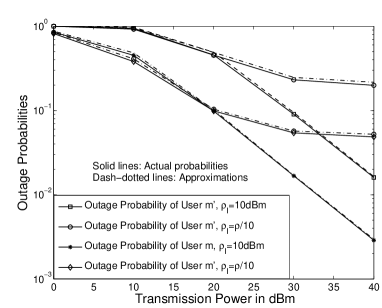
Figure 1: Comparison between $\tilde{\mathrm{P}}_{i^{\prime}}$ and ${\mathrm{P}}_{i^{\prime}}^{o}$, $i\in\{m,m^{\prime}\}$. $R_{m}=R_{m^{\prime}}=1.5$ bit per channel use (BPCU). $\lambda_{I}=10^{-4}$. $r=20$m and $r_{1}=10$m. $r_{0}=1$m and $\alpha_{m^{\prime}}=\frac{3}{4}$. $M=N=2$. The path loss exponent is $\alpha=3$, and the noise power is $-30$dBm.

Given a random choice of $\mathbf{x}_{m}$, the following lemma provides an exact expression for $\tilde{\mathrm{P}}_{m^{\prime}}$ as well as its high SNR approximation.

$\mathbf{Lemma}$ 1.

If $\alpha_{m^{\prime}}^{2}\leq\alpha_{m}^{2}\epsilon_{m^{\prime}}$, the probability $\tilde{\mathrm{P}}_{m^{\prime}}=1$, where $\epsilon_{m^{\prime}}=2^{R_{m^{\prime}}}-1$. Otherwise the probability $\tilde{\mathrm{P}}_{m^{\prime}}$ can be expressed as follows:

$$\tilde{\mathrm{P}}_{m^{\prime}} =1-\frac{2}{r^{2}-r_{1}^{2}}\int_{r_{1}}^{r}e^{-2\phi_{m^{\prime}}x^{\alpha}}\varphi_{I}(x)xdx,$$ (30)

where $\phi_{m^{\prime}}=\frac{\epsilon_{m^{\prime}}}{\rho\alpha_{m^{\prime}}^{2}-\rho\alpha_{m}^{2}\epsilon_{m^{\prime}}}$, $\varphi_{I}(x)=e^{-\pi\lambda_{I}(\beta_{m^{\prime}}(x))^{\frac{2}{\alpha}}\gamma\left(\frac{1}{\alpha},\frac{\beta_{m^{\prime}}(x)}{r_{0}^{\alpha}}\right)}$, $\beta_{m^{\prime}}(x)=2\phi_{m^{\prime}}\delta\rho_{I}L\left(x^{\alpha}\right)$, and $\gamma(\cdot)$ denotes the incomplete Gamma function.

If $\rho_{I}$ is fixed and transmit SNR $\rho$ approaches infinity, the outage probability can be approximated as follows:

$$\tilde{\mathrm{P}}_{m^{\prime}} \approx\frac{2\phi_{m^{\prime}}(2+\tilde{\theta}_{m^{\prime}})}{r^{2}-r_{1}^{2}}\frac{\left(r^{\alpha+2}-r_{1}^{\alpha+2}\right)}{\alpha+2},$$ (31)

where $\tilde{\theta}_{m^{\prime}}=2\pi\lambda_{I}\delta\rho_{I}\frac{\alpha}{r_{0}}$. For the special case of $\rho_{I}=0$, $\tilde{\mathrm{P}}_{m^{\prime}}$ simplifies to

$$\tilde{\mathrm{P}}_{m^{\prime}}=1-\frac{1}{r^{2}-r_{1}^{2}}\left(e^{-2\phi_{m^{\prime}}r^{\alpha}}r^{2}-e^{-2\phi_{m^{\prime}}r_{1}^{\alpha}}r_{1}^{2}\right)-\frac{(2\phi_{m^{\prime}})^{-\frac{2}{\alpha}}}{r^{2}-r_{1}^{2}}\left(\gamma\left(\frac{2}{\alpha}+1,2\phi_{m^{\prime}}r^{\alpha}\right)-\gamma\left(\frac{2}{\alpha}+1,2\phi_{m^{\prime}}r_{1}^{\alpha}\right)\right).$$ (32)

Proof.

Please refer to Appendix A. ∎

By using the high SNR approximation obtained in Lemma 1 and also the fact that both $\phi_{m^{\prime}}$ and $\theta_{m^{\prime}}$ are at the order of $\frac{1}{\rho}$, the achievable diversity gain is obtained in the following corollary.

$\mathbf{Corollary}$ 1.

If $\alpha_{m^{\prime}}^{2}>\alpha_{m}^{2}\epsilon_{m^{\prime}}$, the diversity order achieved by the proposed MIMO-NOMA framework for user $m^{\prime}$ is one.

On the other hand, user $m$ first decodes the message for user $m^{\prime}$ before decoding its own message via SIC. Therefore, the outage probability at user $m$ is given by

$$\mathrm{P}^{o}_{m}=\mathrm{P}\left(\log\left(1+\frac{\rho|h_{m}|^{2}\alpha_{m^{\prime}}^{2}}{\rho|h_{m}|^{2}\alpha_{m}^{2}+|\mathbf{v}_{m}|^{2}+|\mathbf{v}_{m}^{H}\mathrm{1}_{N}|^{2}I_{m}}\right)<R_{m^{\prime}}\right)$$ (33)

$$+\mathrm{P}\left(\log\left(1+\frac{\rho|h_{m}|^{2}\alpha_{m}^{2}}{|\mathbf{v}_{m}|^{2}+|\mathbf{v}_{m}^{H}\mathrm{1}_{N}|^{2}I_{m}}\right)<R_{m},\log\left(1+\frac{\rho|h_{m}|^{2}\alpha_{m^{\prime}}^{2}}{\rho|h_{m}|^{2}\alpha_{m}^{2}+|\mathbf{v}_{m}|^{2}+|\mathbf{v}_{m}^{H}\mathrm{1}_{N}|^{2}I_{m}}\right)>R_{m^{\prime}}\right).$$

Again, we focus on a modified expression for the outage probability as follows:

$$\tilde{\mathrm{P}}_{m} =\mathrm{P}\left(\log\left(1+\frac{\rho|h_{m}|^{2}\alpha_{m^{\prime}}^{2}}{\rho|h_{m}|^{2}\alpha_{m}^{2}+2+2\delta I_{m}}\right)<R_{m^{\prime}}\right)$$ (34)

$$+\mathrm{P}\left(\log\left(1+\frac{\rho|h_{m}|^{2}\alpha_{m}^{2}}{2+2\delta I_{m}}\right)<R_{m},\log\left(1+\frac{\rho|h_{m}|^{2}\alpha_{m^{\prime}}^{2}}{\rho|h_{m}|^{2}\alpha_{m}^{2}+2+2\delta I_{m}}\right)>R_{m^{\prime}}\right),$$

which is an upper bound for $\delta\geq N$ as explained in the proof for Lemma 2. Fig. 1 demonstrates that $\tilde{\mathrm{P}}_{m}$ with a choice of $\delta=1$ yields a tight upper approximation on ${\mathrm{P}}_{m}$. The following lemma provides an exact expression for this probability as well as its high SNR approximation.

$\mathbf{Lemma}$ 2.

If $\alpha_{m^{\prime}}^{2}\leq\alpha_{m}^{2}\epsilon_{m^{\prime}}$, the probability $\tilde{\mathrm{P}}_{m}=1$, otherwise the probability $\tilde{\mathrm{P}}_{m^{\prime}}$ can be expressed as follows:

$$\tilde{\mathrm{P}}_{m} =1-\frac{2}{r_{1}^{2}}\int_{0}^{r_{0}}e^{-2\tilde{\phi}_{m}r_{0}^{\alpha}}\varphi_{I}(r_{0})xdx-\frac{2}{r_{1}^{2}}\int_{r_{0}}^{r_{1}}e^{-2\tilde{\phi}_{m}x^{\alpha}}\varphi_{I}(x)xdx,$$ (35)

where $\tilde{\phi}_{m}=\max\{\phi_{m},\phi_{m^{\prime}}\}$ and $\phi_{m}=\frac{\epsilon_{m}}{\rho\alpha^{2}_{m}}$. If $\rho_{I}$ is fixed and the transmit SNR $\rho$ approaches infinity, the outage probability can be approximated as follows:

$$\tilde{\mathrm{P}}_{m} \approx\frac{\tilde{\phi}_{m}(2+\tilde{\theta}_{m^{\prime}})}{r_{1}^{2}(\alpha+2)}\left(\alpha r_{0}^{\alpha+2}+2r_{1}^{\alpha+2}\right),$$ (36)

where $\tilde{\theta}_{m^{\prime}}$ was defined in Lemma 1.

Proof.

Please refer to Appendix B. ∎

III-B Cognitive Radio Power Allocation

In this section, a cognitive radio inspired power allocation strategy is studied. In particular, assume that user $m^{\prime}$ is viewed as a primary user in a cognitive ratio network. With orthogonal multiple access, the bandwidth resource occupied by user $m^{\prime}$ cannot be reused by other users, despite its poor channel conditions. In contrast, with NOMA, one additional user, i.e., user $m$, can be served simultaneously, under the condition that the QoS requirements of user $m^{\prime}$ can still be met.

In particular, assume that user $m^{\prime}$ needs to achieve a target data rate of $R_{m^{\prime}}$, which means that the power allocation coefficients of NOMA need to satisfy the following constraint

$$\frac{\rho|h_{m^{\prime}}|^{2}\alpha_{m^{\prime}}^{2}}{\rho|h_{m^{\prime}}|^{2}\alpha_{m}^{2}+|\mathbf{v}_{m^{\prime}}|^{2}+|\mathbf{v}_{m^{\prime}}^{H}\mathbf{1}_{N}|^{2}I_{m^{\prime}}}>\epsilon_{m^{\prime}},$$ (37)

which leads to the following choice for $\alpha_{m}$

$$\alpha_{m}^{2}=\max\left(0,\frac{\rho|h_{m^{\prime}}|^{2}-\epsilon_{m^{\prime}}(|\mathbf{v}_{m^{\prime}}|^{2}+|\mathbf{v}_{m^{\prime}}^{H}\mathbf{1}_{N}|^{2}I_{m^{\prime}})}{(1+\epsilon_{m^{\prime}})\rho|h_{m^{\prime}}|^{2}}\right).$$ (38)

It is straightforward to show that $\frac{\rho|h_{m^{\prime}}|^{2}-\epsilon_{m^{\prime}}(|\mathbf{v}_{m^{\prime}}|^{2}+|\mathbf{v}_{m^{\prime}}^{H}\mathbf{1}_{N}|^{2}I_{m^{\prime}})}{(1+\epsilon_{m^{\prime}})\rho|h_{m^{\prime}}|^{2}}$ is always less than one.

An outage at user $m^{\prime}$ means here that all power is allocated to user $m^{\prime}$, but outage still occurs. As a result, the outage probability of user $m^{\prime}$ is exactly the same as that in conventional orthogonal MA systems. Therefore, in this section, we only focus on the outage probability of user $m$ which can be expressed as follows:

$$\mathrm{P}^{o}_{m}= \mathrm{P}\left(|h_{m}|^{2}<\max\left\{\phi_{m^{\prime}}(|\mathbf{v}_{m}|^{2}+|\mathbf{v}_{m}^{H}\mathbf{1}_{N}|^{2}I_{m}),\phi_{m}(|\mathbf{v}_{m}|^{2}+|\mathbf{v}_{m}^{H}\mathbf{1}_{N}|^{2}I_{m})\right\}\right),$$ (39)

if $\alpha_{m^{\prime}}^{2}>\alpha_{m}^{2}\epsilon_{m^{\prime}}$, otherwise outage always occurs. It can be verified that $\alpha_{m^{\prime}}^{2}\leq\alpha_{m}^{2}\epsilon_{m^{\prime}}$ is equivalent to $\alpha_{m}=0$, in the context of cognitive radio power allocation.

Analyzing this outage probability is very difficult due to the following two reasons. First, $h_{m}$ and $\mathbf{v}_{m}$ are correlated, and second, the users experience different but correlated co-channel interference, i.e., $I_{m}\neq I_{m^{\prime}}$. Therefore, in this subsection, we only focus on the case without co-channel interference, i.e., $\rho_{I}=0$. In particular, we focus on the following outage probability

$$\tilde{\mathrm{P}}_{m}= \mathrm{P}\left(|h_{m}|^{2}<2\max\left\{\bar{\phi}_{m^{\prime}},\bar{\phi}_{m}\right\}\right),$$ (40)

where $\bar{\phi}_{m}=\frac{\epsilon_{m}}{\rho\bar{\alpha}^{2}_{m}}$, $\bar{\phi}_{m^{\prime}}=\frac{\epsilon_{m^{\prime}}}{\rho\bar{\alpha}_{m^{\prime}}^{2}-\rho\bar{\alpha}_{m}^{2}\epsilon_{m^{\prime}}}$, and

$$\bar{\alpha}_{m}^{2}=\max\left(0,\frac{\rho|h_{m^{\prime}}|^{2}-2\epsilon_{m^{\prime}}}{(1+\epsilon_{m^{\prime}})\rho|h_{m^{\prime}}|^{2}}\right).$$ (41)

Similarly to the case with fixed power allocation, the outage probability $\tilde{\mathrm{P}}_{m}$ tightly bounds ${\mathrm{P}}^{o}_{m}$. The following lemma provides the expression for the outage probability $\tilde{\mathrm{P}}_{m}$.

$\mathbf{Lemma}$ 3.

When $\rho_{I}=0$, the outage probability can be expressed as follows:

$$\tilde{\mathrm{P}}_{m} =1-\Upsilon_{1}\left(\frac{2\epsilon_{m^{\prime}}}{\rho}\right)\Upsilon_{2}\left(\frac{2\epsilon_{m}(1+\epsilon_{m^{\prime}})}{\rho}\right),$$ (42)

where

$$\Upsilon_{1}(y) =\frac{1}{r^{2}-r_{1}^{2}}\left(e^{-yr^{\alpha}}r^{2}-e^{-yr_{1}^{\alpha}}r_{1}^{2}\right)+\frac{y^{-\frac{2}{\alpha}}}{r^{2}-r_{1}^{2}}\left(\gamma\left(\frac{2}{\alpha}+1,yr^{\alpha}\right)-\gamma\left(\frac{2}{\alpha}+1,yr_{1}^{\alpha}\right)\right).$$ (43)

and

$$\Upsilon_{2}(z) =\frac{r_{0}^{2}e^{-zr_{0}^{\alpha}}}{r_{1}^{2}}+\frac{1}{r_{1}^{2}}\left(e^{-zr_{1}^{\alpha}}r_{1}^{2}-e^{-zr_{0}^{\alpha}}r_{0}^{2}\right)+\frac{z^{-\frac{2}{\alpha}}}{r_{1}^{2}}\left(\gamma\left(\frac{2}{\alpha}+1,zr_{1}^{\alpha}\right)-\gamma\left(\frac{2}{\alpha}+1,zr_{0}^{\alpha}\right)\right).$$

At high SNR, the outage probability can be approximated as follows:

$$\tilde{\mathrm{P}}_{m} \approx\frac{4\epsilon_{m^{\prime}}}{\rho(2+\alpha)(r^{2}-r_{1}^{2})}\left(r^{\alpha+2}-r_{1}^{\alpha+2}\right)+\frac{2r_{0}^{2+\alpha}\epsilon_{m}(1+\epsilon_{m^{\prime}})}{\rho r_{1}^{2}}+\frac{4\epsilon_{m}(1+\epsilon_{m^{\prime}})}{\rho(2+\alpha)r_{1}^{2}}\left(r_{1}^{\alpha+2}-r_{0}^{\alpha+2}\right).$$ (44)

Proof.

Please refer to Appendix C. ∎

Remark 1: By using the above lemma, it is straightforward to show that a diversity gain of one is still achievable at user $m$ (i.e., there is no error floor), and it is important to point out that this is achieved when user $m^{\prime}$ experiences the same outage performance as if it solely uses the channel. Therefore, by using the proposed cognitive radio NOMA, one additional user, user $m$, is introduced into the system to share the spectrum with the primary user, user $m^{\prime}$, without causing any performance degradation at user $m^{\prime}$.

Remark 2: For the above cognitive radio NOMA scheme, it was assumed that the message for user $m^{\prime}$ is decoded first at both receivers. Nevertheless, different SIC decoding strategies can be used, and their impact can be obtained in a straightforward manner from the analysis in the next section, where more complicated uplink transmission schemes are studied. It is worth pointing out that $\alpha_{m}^{2}$ in (38) is always smaller than $\frac{1}{2}$, for $R_{m^{\prime}}\geq 1$. For example, when $\alpha^{2}_{m}=0$, the inequality $\alpha_{m}^{2}-\frac{1}{2}<0$ holds obviously. When $\alpha_{m}^{2}>0$,

$$\alpha_{m}^{2}-\frac{1}{2} =\frac{\rho|h_{m^{\prime}}|^{2}-\epsilon_{m^{\prime}}(|\mathbf{v}_{m}|^{2}+|\mathbf{v}_{m}^{H}\mathbf{1}_{N}|^{2}I_{m^{\prime}})}{(1+\epsilon_{m^{\prime}})\rho|h_{m^{\prime}}|^{2}}-\frac{1}{2}=\frac{\rho|h_{m^{\prime}}|^{2}(1-\epsilon_{m^{\prime}})-2\epsilon_{m^{\prime}}(|\mathbf{v}_{m}|^{2}+|\mathbf{v}_{m}^{H}\mathbf{1}_{N}|^{2}I_{m^{\prime}})}{2(1+\epsilon_{m^{\prime}})\rho|h_{m^{\prime}}|^{2}}\leq 0,$$ (45)

if $R_{m^{\prime}}\geq 1$.

III-C Selection of the User Detection Vectors

Previously, a random choice of $\mathbf{v}_{m}$ and $\mathbf{v}_{m^{\prime}}$ has been used and analyzed. In the case of $2N-M>1$, there is more than one possible choice based on the null space, $\mathbf{U}_{m}$, defined in (11). In this section, we study how to utilize these additional degrees of freedom and analyze their impact on the outage probability.

Finding the optimal choice for $\mathbf{v}_{m}$ and $\mathbf{v}_{m^{\prime}}$ is challenging, since the choice of the detection vectors for one user pair has an impact on those of the other user pairs. For example, the choice of $\mathbf{v}_{m}$ and $\mathbf{v}_{m^{\prime}}$ will affect the $m$-th column of the effective fading matrix $\mathbf{G}$. Recall that the data rates of the users from the $i$-th pair is a function of $\frac{1}{({\mathbf{G}}^{-1}{\mathbf{G}}^{-H})_{i,i}}$. Therefore, the detection vector chosen by the $m$-th user pair will also affect the data rates of the users in the $i$-th pair, $m\neq i$.

In order to avoid this tangled effect, a simple algorithm for detection vector selection is proposed in Table 1. The following lemma shows the diversity gain achieved by the proposed selection algorithm.

Algorithm 1 The selection of the detection vectors $\mathbf{v}_{m}$ and $\mathbf{v}_{m^{\prime}}$

1:  for $i=1$ to $(2N-M)$ do

2:     Set $\mathbf{x}_{m,i}=\begin{bmatrix}\mathbf{0}_{1\times(i-1)}&1&\mathbf{0}_{1\times(M-i)}\end{bmatrix}^{H}$, $\forall m\in\{1,\cdots,M\}$.

3:     Choose the detection vector as $\begin{bmatrix}\mathbf{v}_{m,i}^{H}&\mathbf{v}_{m^{\prime},i}^{H}\end{bmatrix}^{H}=\mathbf{U}_{m}\mathbf{x}_{m,i}$ and determine vector ${\mathbf{g}}_{m,i}=\mathbf{G}_{m}^{H}\mathbf{v}_{m,i}$.

4:     Construct the effective small scale fading matrix, denoted by $\bar{\mathbf{G}}_{i}$, by using $\mathbf{g}_{m,i}$, i.e., $\bar{\mathbf{G}}_{i}=\begin{bmatrix}\mathbf{g}_{1,i}&\cdots&\mathbf{g}_{M,i}\end{bmatrix}^{H}$

5:     Find the effective small scale fading gain for each user pair, $\gamma_{m,i}=\frac{1}{(\bar{\mathbf{G}}_{i}^{-1}\bar{\mathbf{G}}_{i}^{-H})_{m,m}}$.

6:     Find the smallest fading gain, $\gamma_{\min,i}=\min\{\gamma_{1,i},\cdots,\gamma_{M,i}\}$.

7:  end for

8:  Find the index $i$ which maximizes the smallest fading gain, $i^{*}=\underset{i\in{\{1,\cdots,2N-M\}}}{\arg}\max~{}\gamma_{\min,i}$ .

$\mathbf{Lemma}$ 4.

Consider the use of a fixed set of power allocation coefficients. If $\alpha_{m^{\prime}}^{2}\leq\alpha_{m}^{2}\epsilon_{m^{\prime}}$, the probability $\tilde{\mathrm{P}}_{m^{\prime}}=1$, otherwise the use of the algorithm proposed in Table 1 ensures that a diversity gain of $(2N-M)$ is achieved.

Proof.

Please refer to Appendix D. ∎

As can be seen from Lemma 4, the use of the proposed selection algorithm can increase the diversity gain from $1$ to $(2N-M)$, which is a significant improvment compared to the scheme in [13]. Consider a scenario with $N=M$ as an example. The proposed scheme can achieve a diversity gain of $M$, whereas the one in [13] can only achieve a diversity gain of $1$, for an unordered user. Note, however, that the scheme in [13] does not require CSI at the transmitter.

IV Performance Analysis of MIMO-NOMA Uplink Transmission

Because of the symmetry between the uplink and downlink system models of Section II, in this section, we only focus on the difference between two scenarios. One important observation for uplink NOMA is that the sum rate is always the same, no matter which decoding order is used. Therefore, in this section, we first analyze the outage probability with respect to the sum rate for a fixed power allocation. The use of a randomly selected $\mathbf{x}_{m}$ is considered in order to obtain tractable analytical results.

IV-A Fixed Power Allocation

Recall that, if the message from user $m$ is decoded first, the base station can correctly decode the message with rate

$$R_{m,BS,I}=\log\left(1+\frac{\rho|h_{m}|^{2}\alpha^{2}_{m}}{\rho|h_{m^{\prime}}|^{2}\alpha^{2}_{m^{\prime}}+I_{BS,m}+1}\right),$$ (46)

where the interference power is given by

$$I_{BS,m}=\underset{j\in\Psi_{I}}{\sum}\frac{\rho_{I}|\mathbf{p}_{m}^{H}\mathbf{1}_{M}|^{2}}{L\left(d_{I_{j},BS}\right)}.$$ (47)

After subtracting the message from user $m$, the base station can decode the message from user $m^{\prime}$ correctly with the following rate

$$R_{m^{\prime},BS,I}=\log\left(1+\frac{\rho|h_{m^{\prime}}|^{2}\alpha^{2}_{m^{\prime}}}{I_{BS,m}+1}\right).$$ (48)

Therefore, the sum rate achieved by NOMA in the $m$-th sub-channel is given by

$$R_{s} =R_{m,BS,I}+R_{m^{\prime},BS,I}=\log\left(1+\frac{\rho|h|_{m}^{2}\alpha_{m}^{2}+\rho|h|_{m^{\prime}}^{2}\alpha_{m^{\prime}}^{2}}{I_{BS,m}+1}\right).$$ (49)

It is straightforward to verify that the exactly same sum rate is achieved if the message from user $m^{\prime}$ is decoded first. Therefore, the outage probability for the sum rate can be expressed as follows:

$$\mathrm{P}_{s}=\mathrm{P}\left(R_{s}<R_{m}+R_{m^{\prime}}\right).$$ (50)

Note that the term for the interference power contains $|\mathbf{p}_{m}^{H}\mathbf{1}_{M}|^{2}$ which makes the calculation very difficult. Since $|\mathbf{p}_{m}^{H}\mathbf{1}_{M}|^{2}\leq M|\mathbf{p}_{m}^{H}|^{2}=M$, we focus on the following modified expression of the outage probability

$$\tilde{\mathrm{P}}_{s}=\mathrm{P}\left(\log\left(1+\frac{\rho|h|_{m}^{2}\alpha_{m}^{2}+\rho|h|_{m^{\prime}}^{2}\alpha_{m^{\prime}}^{2}}{\delta I_{m}+1}\right)<R_{m}+R_{m^{\prime}}\right),$$ (51)

where $I_{m}=\underset{j\in\Psi_{I}}{\sum}\frac{\rho_{I}}{L\left(d_{I_{j},BS}^{\alpha}\right)}$. Similarly to the downlink case, $\tilde{\mathrm{P}}_{s}$ provides an upper bound on ${\mathrm{P}}_{s}$ for $\delta\geq M$. In the simulation section, we will demonstrate that $\tilde{\mathrm{P}}_{s}$ with a choice of $\delta=1$ provides a tight approximation to ${\mathrm{P}}_{s}$.

Define the small scale fading gain as $x\triangleq\frac{1}{(\mathbf{G}^{-1}\mathbf{G}^{-H})_{m,m}}$. The sum rate outage probability can be expressed as follows

$$\tilde{\mathrm{P}}_{s} =\mathrm{P}\left(\frac{\rho\frac{x}{L(d_{m})}\alpha_{m}^{2}+\rho\frac{x}{L(d_{m^{\prime}})}\alpha_{m^{\prime}}^{2}}{\delta I_{m}+1}<\epsilon\right)=\mathrm{P}\left(x<\frac{\epsilon(\delta I_{m}+1)}{\frac{\rho\alpha_{m}^{2}}{L(d_{m})}+\frac{\rho\alpha_{m^{\prime}}^{2}}{L(d_{m^{\prime}})}}\right),$$ (52)

where $\epsilon=2^{R_{m}+R_{m^{\prime}}}-1$. Following the same steps as in the proof of Lemma 1, the above probability can be expressed as follows:

$$\tilde{\mathrm{P}}_{s} =1-\frac{4}{r_{1}^{2}(r^{2}-r_{1}^{2})}\int_{r_{1}}^{r}\int_{0}^{r_{1}}e^{-\zeta(x,y)}e^{-\pi\lambda_{I}(\rho_{I}\delta\zeta(x,y))^{\frac{2}{\alpha}}\gamma\left(\frac{1}{\alpha},\frac{\rho_{I}\delta\zeta(x,y)}{r_{0}^{\alpha}}\right)}xdxydy,$$ (53)

where $\zeta(d_{m},d_{m^{\prime}})=\frac{\epsilon}{\frac{\rho\alpha_{m}^{2}}{L(d_{m})}+\frac{\rho\alpha_{m^{\prime}}^{2}}{L(d_{m^{\prime}})}}$.

In order to obtain some insights regarding the above probability, we again consider the case that $\rho$ tends to infinity and $\rho_{I}$ is fixed. Since both $d_{m}$ and $d_{m^{\prime}}$ are bounded, $\zeta(d_{m},d_{m^{\prime}})$ approaches zero at high SNR. Therefore the above probability can be approximated as follows:

$$\tilde{\mathrm{P}}_{s} \approx 1-\frac{4}{r_{1}^{2}(r^{2}-r_{1}^{2})}\int_{r_{1}}^{r}\int_{0}^{r_{1}}e^{-\zeta(x,y)}e^{-\pi\lambda_{I}(\rho_{I}\delta\zeta(x,y))^{\frac{2}{\alpha}}\alpha\left(\frac{\rho_{I}\delta\zeta(x,y)}{r_{0}^{\alpha}}\right)^{\frac{1}{\alpha}}}xdxydy$$ (54)

$$\approx 1-\frac{4}{r_{1}^{2}(r^{2}-r_{1}^{2})}\int_{r_{1}}^{r}\int_{0}^{r_{1}}e^{-\zeta(x,y)\left(\frac{\pi\lambda_{I}\alpha\rho_{I}}{r_{0}}+1\right)}xdxydy.$$

With some algebraic manipulations, the above probability can be simplified as follows:

$$\tilde{\mathrm{P}}_{s} \approx 1-\frac{4}{r_{1}^{2}(r^{2}-r_{1}^{2})}\int_{r_{1}}^{r}\int_{0}^{r_{1}}\left(1-\zeta(x,y)\left(\frac{\pi\lambda_{I}\delta\alpha\rho_{I}}{r_{0}}+1\right)\right)xdxydy$$ (55)

$$\approx\frac{4\left(\frac{\pi\lambda_{I}\delta\alpha\rho_{I}}{r_{0}}+1\right)}{r_{1}^{2}(r^{2}-r_{1}^{2})}\int_{r_{1}}^{r}\int_{0}^{r_{1}}\zeta(x,y)xdxydy.$$

Therefore, the outage probability can be approximated as follows:

$$\tilde{\mathrm{P}}_{s} \approx\frac{4\xi\epsilon\left(\frac{\pi\lambda_{I}\delta\alpha\rho_{I}}{r_{0}}+1\right)}{\rho r_{1}^{2}(r^{2}-r_{1}^{2})}\sim\frac{1}{\rho},$$ (56)

where $\xi=\int_{r_{1}}^{r}\int_{0}^{r_{1}}\frac{xy}{\frac{\alpha_{m}^{2}}{L(x)}+\frac{\alpha_{m^{\prime}}^{2}}{L(y)}}dxdy$ is a constant and not related to the SNR. Hence, a diversity gain of $1$ is achievable for the sum rate.

IV-B Cognitive Radio Power Allocation

The design of cognitive radio NOMA for uplink transmission is more complicated, as explained in the following. To simplify the illustration, we omit the interference term in this section, i.e., $\rho_{I}=0$. For downlink transmission, $\alpha_{m}^{2}<\frac{1}{2}$ was sufficient to decide the SIC decoding order. However, there are more uncertainties in the uplink case, since $\alpha_{m^{\prime}}^{2}|h_{m^{\prime}}|^{2}$ is not necessarily larger than $\alpha_{m}^{2}|h_{m}|^{2}$ even if $\alpha_{m^{\prime}}^{2}>\frac{1}{2}$. Therefore, the base station can apply two types of decoding strategies, i.e., it may decode the message from user $m^{\prime}$ first, or that of user $m$ first. These strategies will yield different tradeoffs between the outage performance of the two users, as explained in the following subsections, respectively.

IV-B1 Case I

When the message from user $m^{\prime}$ is decoded first, in order to guarantee the QoS at user $m^{\prime}$, we impose the following power constraint for the power allocation coefficients

$$\log\left(1+\frac{\rho|h_{m^{\prime}}|^{2}\alpha^{2}_{m^{\prime}}}{\rho|h_{m}|^{2}\alpha^{2}_{m}+1}\right)>R_{m^{\prime}},$$ (57)

which leads to the following choice for $\alpha_{m^{\prime}}$

$$\alpha^{2}_{m^{\prime}}=\min\left\{1,\frac{\epsilon_{m^{\prime}}+\rho\epsilon_{m^{\prime}}|h_{m}|^{2}}{\rho|h_{m^{\prime}}|^{2}+\epsilon_{m^{\prime}}\rho|h_{m}|^{2}}\right\}.$$ (58)

Following the same steps as in the proof of Lemma 2, the outage probability $\mathrm{P}^{I}_{m^{\prime},BS}$ can be evaluated as follows:

$$\mathrm{P}^{I}_{m^{\prime},BS} =\mathrm{P}\left(\frac{\epsilon_{m^{\prime}}+\rho\epsilon_{m^{\prime}}|h_{m}|^{2}}{\rho|h_{m^{\prime}}|^{2}+\epsilon_{m^{\prime}}\rho|h_{m}|^{2}}>1\right)$$ (59)

$$=\mathrm{P}\left(|h_{m^{\prime}}|^{2}<\frac{\epsilon_{m^{\prime}}}{\rho}\right)=1-\Upsilon_{1}\left(\frac{\epsilon_{m^{\prime}}}{\rho}\right),$$

and following the same steps as in the proof of Lemma 3, the outage probability $\mathrm{P}^{I}_{m,BS}$ can be evaluated as follows:

$$\mathrm{P}^{I}_{m,BS}= \mathrm{P}\left(\frac{\epsilon_{m^{\prime}}+\rho\epsilon_{m^{\prime}}|h_{m}|^{2}}{\rho|h_{m^{\prime}}|^{2}+\epsilon_{m^{\prime}}\rho|h_{m}|^{2}}>1\right)$$ (60)

$$+\mathrm{P}\left(\frac{\epsilon_{m^{\prime}}+\rho\epsilon_{m^{\prime}}|h_{m}|^{2}}{\rho|h_{m^{\prime}}|^{2}+\epsilon_{m^{\prime}}\rho|h_{m}|^{2}}<1,\log\left(1+\rho|h_{m}|^{2}\frac{\rho|h_{m^{\prime}}|^{2}-\epsilon_{m^{\prime}}}{\rho|h_{m^{\prime}}|^{2}+\epsilon_{m^{\prime}}\rho|h_{m}|^{2}}\right)<R_{m}\right)$$

$$= \mathrm{P}\left(|h_{m^{\prime}}|^{2}<\frac{\epsilon_{m^{\prime}}}{\rho}\right)+\mathrm{P}\left(x>\frac{\epsilon_{m^{\prime}}L(d_{m^{\prime}})}{\rho},x<L(d_{m})\frac{\epsilon_{m}}{\rho}+L(d_{m^{\prime}})\frac{\epsilon_{m^{\prime}}}{\rho}\left(1+\epsilon_{m}\right)\right)$$ (61)

$$= 1-\Upsilon_{1}\left(\frac{\epsilon_{m^{\prime}}\left(1+\epsilon_{m}\right)}{\rho}\right)\Upsilon_{2}\left(\frac{\epsilon_{m}}{\rho}\right).$$

IV-B2 Case II

When the message from user $m$ is decoded first, in order to guarantee the QoS at user $m^{\prime}$, we impose the following power constraint for the power allocation coefficients

$$\log\left(1+\rho|h_{m^{\prime}}|^{2}\alpha^{2}_{m^{\prime}}\right)>R_{m^{\prime}},$$ (62)

which leads to the following choice for $\alpha_{m^{\prime}}$

$$\alpha^{2}_{m^{\prime}}=\min\left\{1,\frac{\epsilon_{m^{\prime}}}{\rho|h_{m^{\prime}}|^{2}}\right\}.$$ (63)

With this choice, we can ensure that the outage probabilities of both users are identical, i.e., ${\mathrm{P}}^{II}_{m,BS}={\mathrm{P}}^{II}_{m^{\prime},BS}$, as explained in the following. The outage events that occur at user $m^{\prime}$ can be divided into the following three events

• $\tilde{E}_{1}$: All the power is allocated to user $m^{\prime}$, i.e., $\alpha_{m^{\prime}}=1$, but the user is still in outage. The NOMA system is degraded to a scenario in which only user $m^{\prime}$ is served.

• $\tilde{E}_{2}$: When $\alpha^{2}_{m^{\prime}}<1$, outage occurs at user $m$, and SIC is stopped.

• $\tilde{E}_{3}$: When $\alpha^{2}_{m^{\prime}}<1$, no outage occurs at user $m$, but outage occurs at user $m^{\prime}$.

It is straightforward to show that $\tilde{E}_{3}$ will not happen, i.e., $\mathrm{P}(\tilde{E}_{3})=0$. Therefore ${\mathrm{P}}_{m^{\prime},BS}=\mathrm{P}(\tilde{E}_{1})+\mathrm{P}(\tilde{E}_{2})$. On the other hand, there are only two outage events for decoding the message from user $m$, which are $\tilde{E}_{1}$ and $\tilde{E}_{2}$, respectively. Therefore, the outage probabilities of the two users are the same, ${\mathrm{P}}_{m,BS}^{II}={\mathrm{P}}^{II}_{m^{\prime},BS}$.

Therefore, we only need to study the outage probability for the message from user $m$. With the choice shown in (63), the outage probability can be rewritten as follows:

$${\mathrm{P}}^{II}_{m,BS} =\mathrm{P}\left(\frac{\epsilon_{m^{\prime}}}{\rho|h_{m^{\prime}}|^{2}}>1\right)+\mathrm{P}\left(\frac{\epsilon_{m^{\prime}}}{\rho|h_{m^{\prime}}|^{2}}<1,\frac{\rho|h_{m}|^{2}\left(1-\frac{\epsilon_{m^{\prime}}}{\rho|h_{m^{\prime}}|^{2}}\right)}{\rho|h_{m^{\prime}}|^{2}\frac{\epsilon_{m^{\prime}}}{\rho|h_{m^{\prime}}|^{2}}+1}<\epsilon_{m}\right).$$ (64)

Therefore, the outage probability can be expressed as follows:

$${\mathrm{P}}^{II}_{m,BS} =\mathrm{P}\left(x<\frac{L(d_{m^{\prime}})\epsilon_{m^{\prime}}}{\rho}\right)+\mathrm{P}\left(\frac{L(d_{m^{\prime}})\epsilon_{m^{\prime}}}{\rho}<x<\frac{L(d_{m^{\prime}})\epsilon_{m^{\prime}}}{\rho}+\frac{\epsilon_{m}\left(\epsilon_{m^{\prime}}+1\right)L(d_{m})}{\rho}\right).$$ (65)

By applying the same steps as in the proof of Lemma 3 for finding $\mathrm{P}(E_{1})$ and $\mathrm{P}(E_{3})$, the outage probability can be obtained as follows:

$${\mathrm{P}}_{m^{\prime},BS}^{II}={\mathrm{P}}_{m,BS}^{II} =1-\Upsilon_{1}\left(\frac{\epsilon_{m^{\prime}}}{\rho}\right)\Upsilon_{2}\left(\frac{\epsilon_{m}(1+\epsilon_{m^{\prime}})}{\rho}\right).$$ (66)

Remark 3: The two considered cases strike different tradeoffs between the outage performance of the two users. Case I can ensure that the QoS at user $m^{\prime}$ is strictly met, and therefore user $m^{\prime}$ will experience a lower outage probability in Case I, which can be confirmed by the fact that ${\mathrm{P}}_{m^{\prime},BS}^{I}<{\mathrm{P}}_{m^{\prime},BS}^{II}$, due to $\Upsilon_{2}\left(\frac{\epsilon_{m}(1+\epsilon_{m^{\prime}})}{\rho}\right)\leq 1$. On the other hand, Case II does not require that the message of user $m^{\prime}$ arrives at the base station with a stronger signal strength since the base station will decode the message from user $m$ first. This is important to avoid the problem of using too much power for compensating the huge path loss of the channel of user $m^{\prime}$. As a result, more power is allcoated to user $m$ compared to Case I, and hence, user $m$ experiences better outage performance in Case II, i.e., ${\mathrm{P}}_{m,BS}^{I}>{\mathrm{P}}_{m,BS}^{II}$. This can be shown by comparing (61) with (65) and by considering

$$L(d_{m})\epsilon_{m}+\epsilon_{m^{\prime}}\left(\epsilon_{m}+1\right)L(d_{m^{\prime}})<L(d_{m^{\prime}})\epsilon_{m^{\prime}}+\epsilon_{m}\left(\epsilon_{m^{\prime}}+1\right)L(d_{m}).$$ (67)

V Numerical Studies

In this section, the performance of the proposed NOMA framework is investigated by using computer simulations. The performance of three benchmark schemes, termed MIMO-OMA without precoding, MIMO-OMA with precoding, and MIMO-NOMA without precoding, is shown in Fig. 2, in order to better illustrate the performance gain of the proposed framework. The design for the two schemes without precoding can be found in [13]. The MIMO-OMA scheme with precoding serves $M$ users during each orthogonal channel use, e.g., one time slot, whereas $2M$ users are served simultaneously by the proposed scheme. For MIMO-OMA with precoding, the design of the detection vectors was obtained by following the algorithm proposed in Table 1, where the users will carry out antenna selection in each iteration. The framework proposed in this paper is termed SA-MIMO-NOMA. The path loss exponent is set as $\alpha=3$. The size of $\mathcal{D}_{1}$ and $\mathcal{D}_{2}$ is determined by $r=20$m, and $r_{1}=10$m. The parameter for the bounded path loss model is set as $r_{0}=1$.

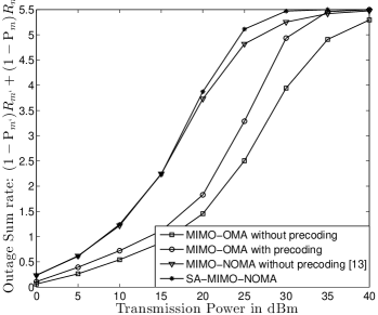
(a) Outage Sum rate

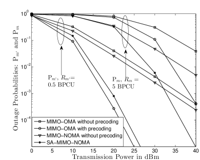
(b) Outage Probabilities

Figure 2: Performance comparison with the three benchmark schemes for downlink transmission. $R_{m}=5$ BPCU and $R_{m^{\prime}}=0.5$ BPCU. $r=20$m and $r_{1}=10$m. $M=N=3$. $r_{0}=1$m. $a_{m^{\prime}}=\frac{3}{4}$. The path loss exponent is $\alpha=3$. The noise power is $-30$dBm and the interference power is $\rho_{I}=0$.

Since the benchmark schemes were proposed for the interference-free scenario, Fig. 2 shows the performance comparison of the four schemes for $\rho_{I}=0$. In Fig. 2(a), the downlink outage sum rate, defined as $R_{m^{\prime}}(1-\mathrm{P}_{m^{\prime}})+R_{m}(1-\mathrm{P}_{m})$, is shown as a function of transmission power, and the corresponding outage probabilities are studied in Fig. 2(b). As can be seen from the figures, the two NOMA schemes can achieve larger outage sum rates compared to the two OMA schemes, which demonstrates the superior spectral efficiency of NOMA. In Fig. 2(b), the two schemes with precoding can achieve better outage performance than the two schemes without precoding, due to the efficient use of the degrees of freedom at the base station. Comparing SA-MIMO-NOMA with the MIMO-NOMA scheme proposed in [13], one can observe that their outage sum rate performances are similar, but SA-MIMO-NOMA can offer much better reception reliability, particularly with high transmission power. In terms of individual outage probability, SA-MIMO-NOMA can ensure a lower outage probability at user $m$, i.e., a smaller $\mathrm{P}_{m}$, compared to the MIMO-OMA scheme with precoding, but results in performance degradation for the outage probability at user $m^{\prime}$, i.e., an increase of $\mathrm{P}_{m^{\prime}}$. This is consistent with the finding in [19] which shows that the NOMA user with poorer channel conditions will suffer some performance loss due to the co-channel interference from its partner.

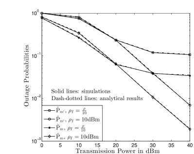
(a) Exact expressions ($R_{m^{\prime}}=R_{m}=1$ BPCU)

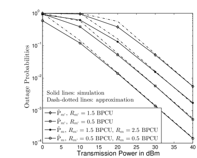
(b) Approximation ($\rho_{I}=-10$dBm)

Figure 3: Outage probabilities $\tilde{\mathcal{P}}_{m^{\prime}}$ and $\tilde{\mathcal{P}}_{m}$ for downlink transmission. $\lambda_{I}=10^{-4}$, $\delta=1$, $r=20$m, $r_{1}=10$m, $M=N=2$, $r_{0}=1$m, and $a_{m^{\prime}}=\frac{3}{4}$. The path loss exponent is $\alpha=3$ and the noise power is $-30$dBm. The analytical results are based on Lemmas 1 and 2.

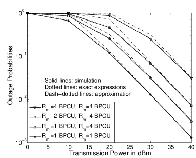
Figure 4: Outage probability $\tilde{\mathrm{P}}_{m}$ for cognitive radio downlink transmission. $r=20$m, $r_{1}=10$m, $r_{0}=1$m, $\delta=1$, $\rho_{I}=0$, and $M=N=2$. The noise power is $-30$dBm. The analytical results and the approximations are based on Lemma 3.

In Fig. 3, the accuracy of the analytical results developed in Lemmas 1 and 2 for downlink transmission is verified. As can be seen from Fig. 3(a), the exact expression developed in Lemma 1 perfectly matches the computer simulations, and the asymptotic results developed in Lemma 1 are also accurate at high SNR, as shown in Fig. 3(b). The accuracy of Lemma 2 can be confirmed similarly. Note that error floors appear when increasing $\rho_{I}$ in Fig. 3(a), which is expected due to the strong co-channel interference caused by the randomly deployed interferers.

In Fig. 4, the performance of the cognitive radio power allocation scheme proposed in Section III-B is studied. In particular, given the target data rate at user $m^{\prime}$, the power allocation coefficients can be calculated opportunistically according to (38). As can be seen from the figure, the probability for this NOMA system to support the secondary user, i.e., user $m$, with a target data rate of $R_{m}$ approaches one at high SNR. Note that with OMA, user $m$ cannot be admitted into the channel occupied by user $m^{\prime}$, and with cognitive radio NOMA, one additional user, user $m$, can be served without degrading the outage performance of the primary user, i.e., user $m^{\prime}$.

In Fig. 5, the impact of the number of user antennas on the outage probability is studied. As can be seen from the figure, by increasing the number of the user antennas, the outage probability is decreased, since the dimension of the null space, $\mathbf{U}_{m}$, defined in (11), is increased and there are more possible choices for the detection vectors. Furthermore, the slope of the outage curves is also increased, which indicates an increase of the achieved diversity order and hence confirms the findings of Lemma 4.

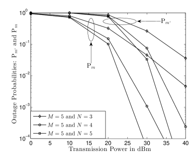
Figure 5: Impact of the number of the user antennas on the downlink outage probabilities ${\mathrm{P}}_{m}$ and ${\mathrm{P}}_{m^{\prime}}$. $R_{m}=4$ BPCU, $R_{m^{\prime}}=1.9$ BPCU, $a_{m^{\prime}}=\frac{3}{4}$, $\rho_{I}=0$, $r=20$m, $r_{1}=10$m, and $r_{0}=1$m. The noise power is $-30$dBm.

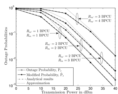
Figure 6: Outage probabilities for the uplink sum rate ${\mathrm{P}}_{s}$ and $\tilde{\mathrm{P}}_{s}$. $r=20$m, $r_{1}=10$m, $r_{0}=1$m, $\delta=1$, $\lambda_{I}=10^{-4}$, $\rho_{I}=10$dB, and $M=N=2$. The noise power is $-30$dBm, and the interference power is $\rho_{I}=-10$dBm. The analytical results and the approximations are based on (53) and (56), respectively.

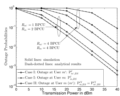
Figure 7: Uplink outage probability for user $m$ with the cognitive radio constraint. $r=4$m, $r_{1}=2$m, $r_{0}=1$m, $\rho_{I}=0$, and the noise power is $-30$dBm. The analytical results and the approximations are based on (60) and (66), respectively.

The performance of the proposed NOMA framework for uplink transmission is demonstrated in Figs. 6 and 7. In particular, in Fig. 6, the outage probability for the sum rate is investigated, and in Fig. 7 the performance of the proposed cognitive radio uplink schemes is studied. As can be observed from both figures, the developed analytical results perfectly match the computer simulation results, which demonstrates the accuracy of the developed analytical framework. It is worth pointing out that the modified probability $\tilde{\mathrm{P}}_{s}$ with $\delta=1$ provides an accurate approximation for $\mathrm{P}_{s}$. An interesting observation from Fig. 7 is that Cases I and II offer different performance advantages. In terms of $\mathrm{P}_{m^{\prime}}$, Case I can offer a lower outage probability compared to Case II, however it results in a loss in outage performance for user $m$. In practice, if the QoS requirement at user $m^{\prime}$ is strict, Case I should be used, since the outage probability realized by Case I is exactly the same as when the entire bandwidth is solely occupied by user $m^{\prime}$. Otherwise, the use of Case II is more preferable since the outage performance for user $m$ can be improved and the system will not spend exceedingly high powers to compensate the user with poorer channel conditions. One can also observe that, for Case I with $R_{m^{\prime}}=R_{m}$, the outage performance for user $m$ is worse than that of user $m^{\prime}$, although user $m$ is closer to the base station. The reason for this is because in Case I, the power is allocated to user $m^{\prime}$ first, and user $m$ is served only if there is any power left. Therefore, the outage probability of user $m$ will be at least the same as that of user $m^{\prime}$, as discussed in Section IV.

VI Conclusions

In this paper, we have proposed a signal alignment based framework which is applicable to both MIMO-NOMA downlink and uplink transmission. By applying tools from stochastic geometry, the impact of the random locations of the users and interferers has been captured, and closed-form expressions for the outage probability achieved by the proposed framework have been developed to facilitate performance evaluation. In addition to fixed power allocation, a more opportunistic power allocation strategy inspired by cognitive ratio networks has also been investigated. Compared to the existing MIMO-NOMA work, the proposed framework is not only more general, i.e., applicable to both uplink and downlink transmissions, but also offers a significant performance gain in terms of reception reliability. In this paper, it has been assumed that global CSI is available, which may introduce a significant training overhead in practice. An important future direction is to study how MIMO-NOMA transmission can be realized with limited CSI feedback.

Appendix A Proof for Lemma 1

First, we rewrite the considered probability $\tilde{\mathrm{P}}_{m^{\prime}}$ as follows:

$$\tilde{\mathrm{P}}_{m^{\prime}}=\mathrm{P}\left(\frac{\frac{\rho\alpha_{m^{\prime}}^{2}}{L(d_{m^{\prime}})(\mathbf{G}^{-1}\mathbf{G}^{-H})_{m,m}}}{\frac{\rho\alpha_{m}^{2}}{L(d_{m^{\prime}})(\mathbf{G}^{-1}\mathbf{G}^{-H})_{m,m}}+2+2\delta I_{m^{\prime}}}<\epsilon_{m^{\prime}}\right).$$ (68)

In order to calculate $\tilde{\mathrm{P}}_{m^{\prime}}$, the density functions for the three parameters, $d_{m^{\prime}}$, $I_{m^{\prime}}$ and $\frac{1}{(\mathbf{G}^{-1}\mathbf{G}^{-H})_{m,m}}$ have to be found. Recall that the factor $\frac{1}{(\mathbf{G}^{-1}\mathbf{G}^{-H})_{m,m}}$ can be written as follows [24]:

$$\frac{1}{(\mathbf{G}^{-1}\mathbf{G}^{-H})_{m,m}}=\mathbf{g}_{m}^{H}\left(\mathbf{I}_{M}-\Theta_{m}\right)\mathbf{g}_{m},$$ (69)

where $\Theta_{m}=\tilde{\mathbf{G}}_{m}(\tilde{\mathbf{G}}_{m}^{H}\tilde{\mathbf{G}}_{m})^{-1}\tilde{\mathbf{G}}_{m}^{H}$ and $\tilde{\mathbf{G}}_{m}$ is obtained from $\mathbf{G}$ by removing its $m$-th row. If $\mathbf{g}_{m}$ is complex Gaussian distributed, the density function of $\frac{1}{(\mathbf{G}^{-1}\mathbf{G}^{-H})_{m,m}}$ will be exponentially distributed. This can be shown as follows. First, note that the projection matrix $(\mathbf{I}_{M}-\Theta_{m})$ is an idempotent matrix and has eigenvalues which are either zero or one. Second, recall that each row of $\mathbf{G}$ is generated from an $M\times 2N$ complex Gaussian matrix $\begin{bmatrix}\mathbf{G}_{m}^{H}&\mathbf{G}_{m^{\prime}}^{H}\end{bmatrix}$, i.e.,

$$\mathbf{g}_{m} =\frac{1}{2}\begin{bmatrix}\mathbf{G}_{m}^{H}&\mathbf{G}_{m^{\prime}}^{H}\end{bmatrix}\begin{bmatrix}\mathbf{v}_{m}^{H}&\mathbf{v}_{m^{\prime}}^{H}\end{bmatrix}^{H}=\frac{1}{2}\begin{bmatrix}\mathbf{G}_{m}^{H}&\mathbf{G}_{m^{\prime}}^{H}\end{bmatrix}\mathbf{U}_{m}\mathbf{x}_{m}.$$ (70)

Hence, provided that $\mathbf{x}_{m}$ is a randomly generated and normalized vector, the application of Proposition 1 in [23] yields the following

$$\mathbf{g}_{m}\quad\sim\quad{\rm CN}(0,\mathbf{I}_{M}),$$ (71)

i.e., $\mathbf{g}_{m}$ is still an $M\times 1$ complex Gaussian (CN) vector. Therefore, $\frac{1}{(\mathbf{G}^{-1}\mathbf{G}^{-H})_{m,m}}$ is indeed exponentially distributed, and the outage probability can be expressed as follows:

$$\tilde{\mathrm{P}}_{m^{\prime}}=\mathcal{E}_{I_{m^{\prime}},d_{m^{\prime}}}\left\{1-e^{-2\phi_{m^{\prime}}L(d_{m^{\prime}})}\underset{Q_{1}}{\underbrace{e^{-2\delta\phi_{m^{\prime}}L(d_{m^{\prime}})I_{m^{\prime}}}}}\right\},$$ (72)

which is conditioned on $\alpha_{m^{\prime}}^{2}>\alpha_{m}^{2}\epsilon_{m^{\prime}}$. Otherwise, $\tilde{\mathrm{P}}_{m^{\prime}}$ is always one.

Since the homogenous PPP $\Psi_{I}$ is stationary, the statistics of the interference seen by user $m^{\prime}$ is the same as that seen by any other receiver, according to Slivnyak’s theorem [25]. Therefore, $I_{m^{\prime}}$ can be equivalently evaluated by focusing on the interference reception seen at a node located at the origin, denoted by $I_{0}=\underset{j\in\Psi_{I}}{\sum}\frac{\rho_{I}}{L\left(d_{I_{j}}\right)}$, where $d_{I_{j}}$ denotes the distance between the origin and the $j$-th interference source. As a result, the expectation of $Q_{1}$ with respect to $I_{m^{\prime}}$ can be expressed as follows: [20], [26]

$$\mathcal{E}_{I_{m^{\prime}}}\left\{Q_{1}\right\} =\mathcal{E}_{I_{m^{\prime}}}\left\{e^{-2\delta\phi_{m^{\prime}}L\left(d_{m^{\prime}}\right)\underset{j\in\Psi_{I}}{\sum}\frac{\rho_{I}}{L\left(d_{I_{j}}\right)}}\right\}={\rm exp}\left(-\lambda_{I}\int_{t\in{\mathcal{R}}^{2}}\left(1-e^{-2\delta\phi_{m^{\prime}}\rho_{I}L\left(d_{m^{\prime}}\right)L(p)}\right)dp\right),$$ (73)

where $p$ denotes the coordinate of the interference source, and $d$ denotes the distance. Note that distance $d$ is determined by the node location $p$. After changing to polar coordinates, the factor $\mathcal{E}_{I_{m^{\prime}}}$ can be calculated as follows:

$$\mathcal{E}_{I_{m^{\prime}}}\left\{Q_{1}\right\} ={\rm exp}\left(-\pi\lambda_{I}r_{0}^{2}\left(1-e^{-\frac{\beta_{m^{\prime}}(d_{m^{\prime}})}{r_{0}^{\alpha}}}\right)\right){\rm exp}\left(-2\pi\lambda_{I}\int_{r_{0}}^{\infty}\left(1-e^{-\frac{\beta_{m^{\prime}}(d_{m^{\prime}})}{x^{\alpha}}}\right)xdx\right)$$

$$={\rm exp}\left(-\pi\lambda_{I}\beta_{m^{\prime}}^{\frac{2}{\alpha}}\gamma\left(\frac{1}{\alpha},\frac{\beta_{m^{\prime}}}{r_{0}^{\alpha}}\right)\right),$$ (74)

where $\beta_{m^{\prime}}(d_{m^{\prime}})$ is denoted by $\beta_{m^{\prime}}$ for notational simplicity. Therefore, the outage probability can be expressed as follows:

$$\tilde{\mathrm{P}}_{m^{\prime}}=1-\mathcal{E}_{d_{m^{\prime}}}\left\{e^{-2\phi_{m^{\prime}}(d_{m^{\prime}}^{\alpha})}\mathcal{E}_{I_{m^{\prime}}}\left\{Q_{1}\right\}\right\}.$$ (75)

Recall that user $m^{\prime}$ is uniformly distributed in the ring $\mathcal{D}_{2}$. Therefore, the above expectation with respect to $d_{m^{\prime}}$ can be calculated as follows:

$$\tilde{\mathrm{P}}_{m^{\prime}}=1-\int_{p\in\mathcal{D}_{2}}e^{-2\phi_{m^{\prime}}L(d_{m^{\prime}})}\mathcal{E}_{I_{m^{\prime}}}\left\{Q_{1}\right\}\frac{dp}{\pi r^{2}-\pi r_{1}^{2}},$$ (76)

where distance $d_{m^{\prime}}$ is determined by the user location $p$. Changing again to polar coordinates, this probability can be expressed as follows:

$$\tilde{\mathrm{P}}_{m^{\prime}} =1-\frac{2}{r^{2}-r_{1}^{2}}\int_{r_{1}}^{r}e^{-2\phi_{m^{\prime}}x^{\alpha}}\mathcal{E}_{I_{m^{\prime}}}\left\{Q_{1}\right\}xdx.$$ (77)

Hence, the first part of the lemma is proved.

In the case that $\rho$ approaches infinity and $\rho_{I}$ is fixed, it is easy to verify that $\phi_{m^{\prime}}$, as well as $\beta_{m^{\prime}}$, go to zero. Hence, the incomplete Gamma function in (74) can be approximated as follows:

$$\gamma\left(\frac{1}{\alpha},\frac{\beta_{m^{\prime}}}{r_{0}^{\alpha}}\right) =\sum^{\infty}_{n=0}\frac{(-1)^{n}\left(\frac{\beta_{m^{\prime}}}{r_{0}^{\alpha}}\right)^{\frac{1}{\alpha}+n}}{n!\left(\frac{1}{\alpha}+n\right)}\approx\alpha\left(\frac{\beta_{m^{\prime}}}{r_{0}^{\alpha}}\right)^{\frac{1}{\alpha}}.$$ (78)

Therefore, the factor $\mathcal{E}_{I_{m^{\prime}}}$ can be approximated as follows:

$$\mathcal{E}_{I_{m^{\prime}}}\left\{Q_{1}\right\} \approx{\rm exp}\left(-\pi\lambda_{I}\beta_{m^{\prime}}^{\frac{2}{\alpha}}\alpha\left(\frac{\beta_{m^{\prime}}}{r_{0}^{\alpha}}\right)^{\frac{1}{\alpha}}\right)\triangleq e^{-d_{m^{\prime}}^{\alpha}\theta_{m^{\prime}}},$$ (79)

where $\theta_{m^{\prime}}=2\pi\lambda_{I}\delta\phi_{m^{\prime}}\rho_{I}\frac{\alpha}{r_{0}}$. Using this approximation the outage probability can be simplified at high SNR as follows:

$$\tilde{\mathrm{P}}_{m^{\prime}} \approx 1-\frac{2}{r^{2}-r_{1}^{2}}\int_{r_{1}}^{r}e^{-2\phi_{m^{\prime}}x^{\alpha}}e^{-x^{\alpha}\theta_{m^{\prime}}}xdx$$ (80)

$$\approx 1-\frac{2}{r^{2}-r_{1}^{2}}\int_{r_{1}}^{r}\left(1-(2\phi_{m^{\prime}}+\theta_{m^{\prime}})x^{\alpha}\right)xdx=\frac{2(2\phi_{m^{\prime}}+\theta_{m^{\prime}})}{r^{2}-r_{1}^{2}}\frac{\left(r^{\alpha+2}-r_{1}^{\alpha+2}\right)}{\alpha+2}.$$

For the special cause without co-channel interfere, i.e., $\rho_{I}=0$, the probability in (77) can be simplified as follows:

$$\tilde{\mathrm{P}}_{m^{\prime}} =1-\frac{2}{r^{2}-r_{1}^{2}}\int_{r_{1}}^{r}e^{-2\phi_{m^{\prime}}x^{\alpha}}xdx=1-\frac{1}{r^{2}-r_{1}^{2}}\int^{r^{\alpha}}_{r_{1}^{\alpha}}e^{-2\phi_{m^{\prime}}y}dy^{\frac{2}{\alpha}}$$ (81)

$$=1-\frac{e^{-2\phi_{m^{\prime}}}}{r^{2}-r_{1}^{2}}\left(e^{-r^{\alpha}}r^{2}-e^{-r_{1}^{\alpha}}r_{1}^{2}\right)-\frac{(2\phi_{m^{\prime}})^{-\frac{2}{\alpha}}}{r^{2}-r_{1}^{2}}\left(\gamma\left(\frac{2}{\alpha}+1,2\phi_{m^{\prime}}r^{\alpha}\right)-\gamma\left(\frac{2}{\alpha}+1,2\phi_{m^{\prime}}r_{1}^{\alpha}\right)\right),$$

and the lemma is proved.

Appendix B Proof for Lemma 2

When $\alpha_{m^{\prime}}^{2}>\alpha_{m}^{2}\epsilon_{m^{\prime}}$, the outage probability $\tilde{\mathrm{P}}_{m}$ can be written as follows:

$$\tilde{\mathrm{P}}_{m} =\mathrm{P}\left(|h_{m}|^{2}<2\phi_{m^{\prime}}(1+\delta I_{m})\right)+\mathrm{P}\left(|h_{m}|^{2}<2\phi_{m}(1+\delta I_{m}),|h_{m}|^{2}>2\phi_{m^{\prime}}(1+\delta I_{m})\right)$$ (82)

$$=\mathrm{P}\left(|h_{m}|^{2}<2\max\{\phi_{m},\phi_{m^{\prime}}\}(1+\delta I_{m})\right),$$

The reason why $\tilde{\mathrm{P}}_{m}$ is an upper bound on ${\mathrm{P}}^{o}_{m}$ for $\delta\geq N$ can be explained as follows. Recall that the original outage probability $\mathrm{P}^{o}_{m}$ can be expressed as ${\mathrm{P}}^{o}_{m}=\mathrm{P}\left(|h_{m}|^{2}<\max\{\phi_{m},\phi_{m^{\prime}}\}(|\mathbf{v}_{m}|^{2}+|\mathbf{v}_{m}^{H}\mathbf{1}_{N}|^{2}I_{m})\right)$. Since $|\mathbf{v}_{m}^{H}\mathbf{1}_{N}|^{2}\leq N|\mathbf{v}_{m}|^{2}$ and $|\mathbf{v}_{m}|^{2}\leq 2$, we have $\mathrm{P}^{o}_{m}\leq\tilde{\mathrm{P}}_{m}$ if $\delta\geq N$. It is worth pointing out that a choice of $\delta=1$ is sufficient to yield a tight approximation on $\mathrm{P}^{o}_{m}$, as shown in Fig. 1.

Recall that $h_{m}=\frac{1}{\sqrt{L(d_{m})(\mathbf{G}^{-1}\mathbf{G}^{-H})_{m,m}}}$. Comparing $h_{m}$ to $h_{m^{\prime}}$, we find that the only difference between the two is the distance $d_{m}$ which is less than $r_{1}$. In addition, the statistics of $I_{m}$ can be studied by using $I_{0}$ as explained in the proof of Lemma 1. Therefore, following steps similar to those in the proof of Lemma 1, the outage probability can be expressed as follows:

$$\tilde{\mathrm{P}}_{m}=\mathcal{E}_{I_{m},d_{m}}\left\{1-e^{-2\tilde{\phi}_{m}L(d_{m})}\underset{Q_{2}}{\underbrace{e^{-2\tilde{\phi}_{m}L(d_{m})I_{m}}}}\right\}.$$ (83)

It is straightforward to show that the expectation of $Q_{2}$ can be obtained in the same way as that of $Q_{1}$, by replacing $\phi_{m^{\prime}}$ with $\tilde{\phi}_{m}$. In addition, recall that user $m$ is uniformly distributed in the disc $\mathcal{D}_{1}$. Therefore, the outage probability can be calculated as follows:

$$\tilde{\mathrm{P}}_{m}=1-\int_{p\in\mathcal{D}_{1}}e^{-2\tilde{\phi}_{m}L(d_{m})}\varphi_{I}(L(d_{m}))\frac{dp}{\pi r_{1}^{2}},$$ (84)

where distance $d_{m}$ is again determined by the user location $p$. Resorting to polar coordinates, the outage probability can be expressed as follows:

$$\tilde{\mathrm{P}}_{m} =1-\frac{2}{r_{1}^{2}}\int_{0}^{r_{0}}e^{-2\tilde{\phi}_{m}r_{0}^{\alpha}}\varphi_{I}(L(x)xdx-\frac{2}{r_{1}^{2}}\int_{r_{0}}^{r_{1}}e^{-2\tilde{\phi}_{m}x^{\alpha}}\varphi_{I}(L(x))xdx.$$ (85)

If $\rho$ approaches infinity and $\rho_{I}$ is fixed, both $\beta_{m}$ and $\tilde{\phi}_{m}$ go to zero. With this approximation, the incomplete Gamma function in (74) can be approximated as $\mathcal{E}_{I_{m}}\left\{Q_{1}\right\}\approx e^{-d_{m}^{\alpha}{\theta}_{m}}$, where $\theta_{m}=2\pi\lambda_{I}\tilde{\phi}_{m}\rho_{I}\frac{\alpha}{r_{0}}$. Hence, the outage probability can be simplified at high SNR as follows:

$$\tilde{\mathrm{P}}_{m} \approx 1-\frac{2}{r_{1}^{2}}\int_{0}^{r_{0}}e^{-2\tilde{\phi}_{m}r_{0}^{\alpha}}e^{-r_{0}^{\alpha}\theta_{m}}xdx-\frac{2}{r_{1}^{2}}\int_{r_{0}}^{r_{1}}e^{-2\tilde{\phi}_{m}x^{\alpha}}e^{-x^{\alpha}\theta_{m}}xdx$$ (86)

$$\approx 1-\frac{r_{0}^{2}}{r_{1}^{2}}\left(1-2\tilde{\phi}_{m}r_{0}^{\alpha}-r_{0}^{\alpha}\theta_{m}\right)-\frac{2}{r_{1}^{2}}\int_{r_{0}}^{r_{1}}\left(1-(2\tilde{\phi}_{m}+\theta_{m})x^{\alpha}\right)xdx$$

$$\approx\frac{(2\tilde{\phi}_{m}+\theta_{m})}{r_{1}^{2}(\alpha+2)}\left(\alpha r_{0}^{\alpha+2}+2r_{1}^{\alpha+2}\right),$$

and the lemma is proved.

Appendix C Proof for Lemma 3

There are three types of outage events at user $m$, as illustrated in the following:

• $\bar{\alpha}_{m}^{2}=0$, i.e., all the power is consumed by user $m^{\prime}$ and no power is allocated to user $m$. This event is denoted by $E_{1}$.

• When $\bar{\alpha}_{m}^{2}>0$, user $m$ cannot decode the message to user $m^{\prime}$. This event is denoted by $E_{2}$.

• When $\bar{\alpha}_{m}^{2}>0$, user $m$ can decode the message to user $m^{\prime}$, but fails to decode its own message. This event is denoted by $E_{3}$.

The probability of $E_{1}$ can be expressed as follows:

$$\mathrm{P}(E_{1})=\mathrm{P}\left(\rho|h_{m^{\prime}}|^{2}-2\epsilon_{m^{\prime}}<0\right).$$ (87)

This probability can be straightforwardly obtained from the proof of Lemma 1 by replacing $\phi_{m^{\prime}}$ with $\breve{\phi}_{m^{\prime}}\triangleq\frac{2\epsilon_{m^{\prime}}}{\rho}$. Therefore, $\mathrm{P}(E_{1})$ can be expressed as follows:

$${\mathrm{P}}(E_{1})=1-\Upsilon_{1}\left(\frac{2\epsilon_{m^{\prime}}}{\rho}\right).$$ (88)

When $\bar{\alpha}_{m}>0$, $\mathrm{P}(E_{2})=0$, since

$$\mathrm{P}(E_{2})= \mathrm{P}\left(\frac{\rho|h_{m}|^{2}(1-\bar{\alpha}_{m}^{2})}{\rho|h_{m}|^{2}\bar{\alpha}_{m}^{2}+2}<\epsilon_{m^{\prime}}\right)=\mathrm{P}\left(\rho|h_{m}|^{2}(1-\bar{\alpha}_{m}^{2})<\epsilon_{m^{\prime}}(\rho|h_{m}|^{2}\bar{\alpha}_{m}^{2}+2)\right)$$ (89)

$$= \mathrm{P}\left(\rho|h_{m}|^{2}<\bar{\alpha}_{m}^{2}\rho|h_{m}|^{2}(1+\epsilon_{m^{\prime}})+2\epsilon_{m^{\prime}}\right)$$

$$= \mathrm{P}\left(\rho|h_{m}|^{2}|h_{m^{\prime}}|^{2}<\rho|h_{m^{\prime}}|^{2}|h_{m}|^{2}-2|h_{m}|^{2}\epsilon_{m^{\prime}}+2|h_{m^{\prime}}|^{2}\epsilon_{m^{\prime}}\right)=\mathrm{P}\left(|h_{m}|^{2}<|h_{m^{\prime}}|^{2}\right)=0.$$

The probability for event $E_{3}$ can be calculated as follows:

$$\mathrm{P}(E_{3}) =\mathrm{P}\left(\log\left(1+\frac{\rho}{2}|h_{m}|^{2}\alpha_{m}^{2}\right)<R_{m},\bar{\alpha}_{m}>0\right)=\mathrm{P}\left(|h_{m}|^{2}\frac{\rho|h_{m^{\prime}}|^{2}-2\epsilon_{m^{\prime}}}{2(1+\epsilon_{m^{\prime}})|h_{m^{\prime}}|^{2}}<\epsilon_{m},|h_{m^{\prime}}|^{2}>\frac{2\epsilon_{m^{\prime}}}{\rho}\right).$$ (90)

An important observation is that both channel gains $h_{m}$ and $h_{m^{\prime}}$ share the same small scale fading. Defining $x=\frac{1}{(\mathbf{G}^{-1}\mathbf{G}^{-H})_{m,m}}$, the outage probability can be expressed as follows:

$$\mathrm{P}(E_{3}) =\mathrm{P}\left(\frac{x}{L(d_{m})}\frac{\rho\frac{x}{L(d_{m^{\prime}})}-2\epsilon_{m^{\prime}}}{(1+\epsilon_{m^{\prime}})\frac{x}{L(d_{m^{\prime}})}}<2\epsilon_{m},\frac{x}{L(d_{m^{\prime}})}>\frac{2\epsilon_{m^{\prime}}}{\rho}\right)$$ (91)

$$=\mathrm{P}\left(\frac{2\epsilon_{m^{\prime}}L(d_{m^{\prime}})}{\rho}<x<\frac{2\epsilon_{m^{\prime}}L(d_{m^{\prime}})}{\rho}+\frac{2\epsilon_{m}(1+\epsilon_{m^{\prime}})L(d_{m})}{\rho}\right).$$

The above probability can be calculated as follows

$$\mathrm{P}(E_{3}) =\underset{p_{m^{\prime}}\in\mathcal{D}_{2}}{\int}e^{-\frac{2\epsilon_{m^{\prime}}L(d_{m^{\prime}})}{\rho}}dp_{m^{\prime}}-\underset{p_{m}\in\mathcal{D}_{1},p_{m^{\prime}}\in\mathcal{D}_{2}}{\int\int}e^{-\frac{2\epsilon_{m^{\prime}}L(d_{m^{\prime}})}{\rho}-\frac{2\epsilon_{m}(1+\epsilon_{m^{\prime}})L(d_{m})}{\rho}}dp_{m}dp_{m^{\prime}},$$ (92)

where $p_{m}$ denotes the location of user $m$. Since the users are uniformly distributed, the above probability can be expressed as follows:

$$\mathrm{P}(E_{3}) =\frac{2}{(r^{2}-r_{1}^{2})}\int_{r_{1}}^{r}e^{-\frac{2\epsilon_{m^{\prime}}}{\rho y^{\alpha}}}ydy-\frac{4}{r_{1}^{2}(r^{2}-r_{1}^{2})}\int_{0}^{r_{1}}e^{-\frac{2\epsilon_{m}(1+\epsilon_{m^{\prime}})}{\rho y^{\alpha}}}ydy\int_{r_{1}}^{r}e^{-\frac{2\epsilon_{m^{\prime}}L(x)}{\rho}}xdx$$ (93)

$$=\Upsilon_{1}\left(\frac{2\epsilon_{m^{\prime}}}{\rho}\right)-\Upsilon_{1}\left(\frac{2\epsilon_{m^{\prime}}}{\rho}\right)\Upsilon_{2}\left(\frac{2\epsilon_{m}(1+\epsilon_{m^{\prime}})}{\rho}\right).$$

Combining (88), (89), and (93), the first part of the lemma can be proved. To obtain the high SNR approximation, we have

$$\Upsilon_{1}(y) \approx 1+\frac{1}{r^{2}-r_{1}^{2}}\left(yr_{1}^{\alpha+2}-yr^{\alpha+2}\right)+\frac{y^{-\frac{2}{\alpha}}}{(\frac{2}{\alpha}+1)(r^{2}-r_{1}^{2})}\left(\left(yr^{\alpha}\right)^{\frac{2}{\alpha}+1}-\left(yr_{1}^{\alpha}\right)^{\frac{2}{\alpha}+1}\right)$$ (94)

$$=1-\frac{2y}{(2+\alpha)(r^{2}-r_{1}^{2})}\left(r^{\alpha+2}-r_{1}^{\alpha+2}\right),$$

when $y$ approaches zero, and

$$\Upsilon_{2}(z) \approx 1-\frac{r_{0}^{2+\alpha}z}{r_{1}^{2}}-\frac{1}{r_{1}^{2}}\left(zr_{1}^{\alpha+2}-zr_{0}^{\alpha+2}\right)+\frac{z^{-\frac{2}{\alpha}}}{(\frac{2}{\alpha}+1)r_{1}^{2}}\left(\left(zr_{1}^{\alpha}\right)^{\frac{2}{\alpha}+1}-\left(zr_{0}^{\alpha}\right)^{\frac{2}{\alpha}+1}\right)$$

$$=1-\frac{r_{0}^{2+\alpha}z}{r_{1}^{2}}-\frac{2z}{(2+\alpha)r_{1}^{2}}\left(r_{1}^{\alpha+2}-r_{0}^{\alpha+2}\right),$$ (95)

when $z$ approaches zero. By substituting the above approximations into (42), the lemma is proved.

Appendix D Proof for Lemma 4

We focus on the outage performance of user $m^{\prime}$ first. Given the detection vector $\mathbf{v}_{m,i^{*}}$ chosen from Table 1, the outage probability can be upper bounded as follows:

$${\mathrm{P}}_{m^{\prime},i^{*}} \leq\mathrm{P}\left(\frac{\frac{\rho\alpha_{m^{\prime}}^{2}}{L(d_{m^{\prime}})(\bar{\mathbf{G}}_{i^{*}}^{-1}\bar{\mathbf{G}}_{i^{*}}^{-H})_{m,m}}}{\frac{\rho\alpha_{m}^{2}}{L(d_{m^{\prime}})(\bar{\mathbf{G}}_{i^{*}}^{-1}\bar{\mathbf{G}}_{i^{*}}^{-H})_{m,m}}+2+2\delta I_{m^{\prime}}}<\epsilon_{m^{\prime}}\right)$$

$$=\mathrm{P}\left(\gamma_{m,{i^{*}}}<2\phi_{m^{\prime}}L(d_{m^{\prime}})(1+\delta I_{m^{\prime}})\right)\leq\mathrm{P}\left(\gamma_{{\rm min},{i^{*}}}<2\phi_{m^{\prime}}L(d_{m^{\prime}})(1+\delta I_{m^{\prime}})\right).$$ (96)

According to the algorithm proposed in Table 1,

$$\gamma_{{\rm min},i^{*}}=\max\{\gamma_{{\rm min},1},\cdots,\gamma_{{\rm min},2N-M}\}.$$ (97)

Therefore, the outage probability can be bounded as follows:

$${\mathrm{P}}_{m^{\prime},i^{*}} \leq\left(\mathrm{P}\left(\gamma_{{\rm min},i}<2\phi_{m^{\prime}}L(d_{m^{\prime}})(1+\delta I_{m^{\prime}})\right)\right)^{2N-M},$$

where the inequality follows from the fact that $\gamma_{{\rm min},i}$ and $\gamma_{{\rm min},j}$ are independent, since $\mathbf{g}_{m,i}$ and $\mathbf{g}_{m,j}$ are independent (Proposition 1 in [23]). The above outage probability can be further bounded as follows:

$${\mathrm{P}}_{m^{\prime},i^{*}} \leq\left(M\mathrm{P}\left(\gamma_{m,i}<2\phi_{m^{\prime}}L(d_{m^{\prime}})(1+\delta I_{m^{\prime}})\right)\right)^{2N-M}.$$ (98)

Following the same steps as in the proof of Lemma 1, the upper bound on the outage probability can be calculated as follows:

$${\mathrm{P}}_{m^{\prime},i^{*}} \leq M^{2N-M}\mathcal{E}_{I_{m^{\prime}},d_{m^{\prime}}}\left\{\left(1-e^{-2\phi_{m^{\prime}}L(d_{m^{\prime}})}e^{-2\delta\phi_{m^{\prime}}L(d_{m^{\prime}})I_{m^{\prime}}}\right)^{2N-M}\right\}$$ (99)

$$\leq M^{2N-M}\sum^{2N-M}_{i=0}{2N-M\choose i}(-1)^{i}\mathcal{E}_{I_{m^{\prime}},d_{m^{\prime}}}\left\{e^{-2i\phi_{m^{\prime}}L(d_{m^{\prime}})}e^{-2i\delta\phi_{m^{\prime}}L(d_{m^{\prime}})I_{m^{\prime}}}\right\},$$

which is conditioned on $\alpha_{m^{\prime}}^{2}>\alpha_{m}^{2}\epsilon_{m^{\prime}}$.

After the expectation with respect to $I_{m^{\prime}}$, the outage probability can be bounded as follows:

$${\mathrm{P}}_{m^{\prime},i^{*}} \leq M^{2N-M}\sum^{2N-M}_{i=0}{2N-M\choose i}(-1)^{i}\mathcal{E}_{d_{m^{\prime}}}\left\{e^{-2i\phi_{m^{\prime}}L(d_{m^{\prime}})}e^{-\pi\lambda_{I}(i\beta_{m^{\prime}})^{\frac{2}{\alpha}}\gamma\left(\frac{1}{\alpha},\frac{i\beta_{m^{\prime}}}{r_{0}^{\alpha}}\right)}\right\}.$$ (100)

For the case of $\rho$ approaching infinity and a fixed $\rho_{I}$, the upper bound on the outage probability can be approximated as follows:

$${\mathrm{P}}_{m^{\prime},i^{*}} \leq M^{2N-M}\sum^{2N-M}_{i=0}{2N-M\choose i}(-1)^{i}\mathcal{E}_{d_{m^{\prime}}}\left\{e^{-2i\phi_{m^{\prime}}L(d_{m^{\prime}})}e^{-\pi\lambda_{I}(i\beta_{m^{\prime}})^{\frac{2}{\alpha}}\alpha\left(\frac{i\beta_{m^{\prime}}}{r_{0}^{\alpha}}\right)^{\frac{1}{\alpha}}}\right\}$$ (101)

$$\leq M^{2N-M}\sum^{2N-M}_{i=0}{2N-M\choose i}(-1)^{i}\mathcal{E}_{d_{m^{\prime}}}\left\{e^{-(i\theta_{m^{\prime}}+2i\phi_{m^{\prime}})d_{m}^{\alpha}}\right\}.$$

Using polar coordinates, the upper bound can be calculated as follows:

$${\mathrm{P}}_{m^{\prime},i^{*}} \leq M^{2N-M}\sum^{2N-M}_{i=0}{2N-M\choose i}(-1)^{i}\frac{2}{r^{2}-r_{1}^{2}}\sum^{\infty}_{j=0}\int_{r_{1}}^{r}\frac{(-1)^{j}(i\theta_{m^{\prime}}+2i\phi_{m^{\prime}})^{j}x^{j\alpha}}{j!}xdx$$ (102)

$$=\frac{2M^{2N-M}}{r^{2}-r_{1}^{2}}\sum^{2N-M}_{i=0}{2N-M\choose i}(-1)^{i}\sum^{\infty}_{j=0}\frac{(-1)^{j}(i\theta_{m^{\prime}}+2i\phi_{m^{\prime}})^{j}}{j!}\frac{\left(r^{j\alpha+2}-r_{1}^{j\alpha+2}\right)}{j\alpha+2}.$$ (103)

By exchanging the two sums in the above equation, the upper bound can be rewritten as follows:

$${\mathrm{P}}_{m^{\prime},i^{*}} \leq\frac{2M^{2N-M}}{r^{2}-r_{1}^{2}}\sum^{\infty}_{j=0}\frac{(-1)^{j}(\theta_{m^{\prime}}+2\phi_{m^{\prime}})^{j}}{j!}\frac{\left(r^{j\alpha+2}-r_{1}^{j\alpha+2}\right)}{j\alpha+2}\sum^{2N-M}_{i=0}{2N-M\choose i}(-1)^{i}i^{j}$$ (104)

$$=\frac{2M^{2N-M}}{r^{2}-r_{1}^{2}}\sum^{\infty}_{j=2N-M}\frac{(-1)^{j}(\theta_{m^{\prime}}+2\phi_{m^{\prime}})^{j}}{j!}\frac{\left(r^{j\alpha+2}-r_{1}^{j\alpha+2}\right)}{j\alpha+2}\sum^{2N-M}_{i=0}{2N-M\choose i}(-1)^{i}i^{j},$$ (105)

where the last step follows from the following fact

$$\sum^{2N-M}_{i=0}{2N-M\choose i}(-1)^{i}i^{j}=0$$

for $0\leq j\leq(2N-M-1)$ [27]. Furthermore, note that both $\phi_{m^{\prime}}$ and $\theta_{m^{\prime}}$ approach zero for the considered scenario, and $\sum^{2N-M}_{i=0}{2N-M\choose i}(-1)^{i}i^{2N-M}=(-1)^{2N-M}(2N-M)!$. Therefore, the upper bound on the outage probability can be approximated as follows:

$${\mathrm{P}}_{m^{\prime},i^{*}}\leq\frac{2M^{2N-M}}{r^{2}-r_{1}^{2}}\frac{(-1)^{2N-M}(\theta_{m^{\prime}}+2\phi_{m^{\prime}})^{2N-M}}{(2N-M)!}\frac{\left(r^{(2N-M)\alpha+2}-r_{1}^{(2N-M)\alpha+2}\right)}{(2N-M)\alpha+2}(-1)^{2N-M}(2N-M)!$$ (106)

$$=\frac{2[M(\theta_{m^{\prime}}+2\phi_{m^{\prime}})]^{2N-M}\left(r^{(2N-M)\alpha+2}-r_{1}^{(2N-M)\alpha+2}\right)}{(r^{2}-r_{1}^{2})((2N-M)\alpha+2)}\sim\frac{1}{\rho^{2N-M}}.$$

The result for user $m$ can be proved using steps similar to the ones above.

The result for a random detection vector can be obtained by replacing $(2N-M)$ with $1$ in the above expression, and the corresponding upper bound becomes

$${\mathrm{P}}_{m^{\prime},i^{*}}\leq\frac{2M[\theta_{m^{\prime}}+2\phi_{m^{\prime}}]\left(r^{\alpha+2}-r_{1}^{\alpha+2}\right)}{(r^{2}-r_{1}^{2})(\alpha+2)}.$$ (107)

which is exactly the same result as the one shown in Lemma 1, except for the extra term $M$ which was introduced by upper bounding the outage probability in (98). Hence, the proof is completed.

References

- [1] Y. Saito, Y. Kishiyama, A. Benjebbour, T. Nakamura, A. Li, and K. Higuchi, “Non-orthogonal multiple access (NOMA) for cellular future radio access,” in Proc. IEEE Vehicular Technology Conference, Dresden, Germany, Jun. 2013.
- [2] Y. Saito, A. Benjebbour, Y. Kishiyama, and T. Nakamura, “System level performance evaluation of downlink non-orthogonal multiple access (NOMA),” in Proc. IEEE Annual Symposium on Personal, Indoor and Mobile Radio Communications (PIMRC), London, UK, Sept. 2013.
- [3] Z. Ding, Z. Yang, P. Fan, and H. V. Poor, “On the performance of non-orthogonal multiple access in 5G systems with randomly deployed users,” IEEE Signal Process. Letters, vol. 21, no. 12, pp. 1501–1505, Dec 2014.
- [4] 3rd Generation Partnership Project(3GPP), “Study on downlink multiuser superposition transmission for LTE,” Mar. 2015.
- [5] “5G radio access: requirements, concepts and technologies,” NTT DOCOMO, Inc., Tokyo, Japan, 5G Whitepaper, Jul. 2014.
- [6] “Proposed solutions for new radio access,” Mobile and wireless communications Enablers for the Twenty-twenty Information Society (METIS), Deliverable D.2.4, Feb. 2015.
- [7] S. Timotheou and I. Krikidis, “Fairness for non-orthogonal multiple access in 5G systems,” IEEE Signal Process. Letters, vol. 22, no. 10, pp. 1647–1651, Oct. 2015.
- [8] V. Kalokidou, O. Johnson, and R. Piechocki, “A hybrid TIM-NOMA scheme for the SISO broadcast channel,” in Proc. IEEE International Conference on Commun. (ICC), Jun. 2015.
- [9] M. Al-Imari, P. Xiao, M. A. Imran, and R. Tafazolli, “Uplink non-orthogonal multiple access for 5G wireless networks,” in Proc. 11th International Symposium on Wireless Communications Systems (ISWCS), Barcelona, Spain, Aug 2014, pp. 781–785.
- [10] H. Marshoud, V. M. Kapinas, G. K. Karagiannidis, and S. Muhaidat, “Non-orthogonal multiple access for visible light communications,” arXiv preprint, Available on-line at arxiv.org/abs/1504.00934.
- [11] J. Choi, “Minimum power multicast beamforming with superposition coding for multiresolution broadcast and application to NOMA systems,” IEEE Trans. Commun., vol. 63, no. 3, pp. 791–800, Mar. 2015.
- [12] Q. Sun, S. Han, C.-L. I, and Z. Pan, “On the ergodic capacity of MIMO NOMA systems,” IEEE Wireless Commun. Letters, (to appear in 2015).
- [13] Z. Ding, F. Adachi, and H. V. Poor, “The application of MIMO to non-orthogonal multiple access,” IEEE Trans. Wireless Commun., (to appear in 2015) Available on-line at arXiv:1503.05367.
- [14] K. Higuchi and Y. Kishiyama, “Non-orthogonal access with random beamforming and intra-beam SIC for cellular MIMO downlink,” in Proc. IEEE Vehicular Technology Conference, Las Vegas, NV, US, Sept. 2013, pp. 1–5.
- [15] N. Lee, J.-B. Lim, and J. Chun, “Degrees of the freedom of the MIMO Y channel: Signal space alignment for network coding,” IEEE Trans Inform. Theory, vol. 56, pp. 3332 – 3343, Jul. 2010.
- [16] Z. Ding and H. Poor, “A general framework of precoding design for multiple two-way relaying communications,” IEEE Trans. Signal Process., vol. 61, no. 6, pp. 1531–1535, Mar. 2013.
- [17] M. Peng, C. Wang, J. Li, H. Xiang, and V. Lau, “Recent advances in underlay heterogeneous networks: Interference control, resource allocation, and self-organization,” IEEE Commun. Surveys Tuts., vol. 17, no. 2, pp. 700–729, Second quarter 2015.
- [18] “C-RAN: The road towards green RAN,” China Mobile Res. Inst., Beijing, China, Oct. 2011, White Paper, ver. 2.5.
- [19] Z. Ding, P. Fan, and H. V. Poor, “Impact of user pairing on 5G non-orthogonal multiple access,” IEEE Trans. Vehicular Technology, (submitted) Available on-line at arXiv:1412.2799.
- [20] M. Haenggi, Stochastic Geometry for Wireless Networks. Cambridge University Press, Cambridge, UK, 2012.
- [21] J. Venkataraman, M. Haenggi, and O. Collins, “Shot noise models for outage and throughput analyses in wireless ad hoc networks,” in Proc. IEEE Military Communications Conference, Washington, DC, USA, Oct. 2006.
- [22] N. Lee and J.-B. Lim, “A novel signaling for communication on MIMO Y channel: Signal space alignment for network coding,” in Proc. IEEE International Symposium on Inform. Theory (ISIT-09), Jul. 2009.
- [23] Z. Ding, T. Wang, M. Peng, and W. Wang, “On the design of network coding for multiple two-way relaying channels,” IEEE Trans. Wireless Commun., vol. 10, no. 6, pp. 1820–1832, Jun. 2011.
- [24] M. Rupp, C. Mecklenbrauker, and G. Gritsch, “High diversity with simple space time block codes and linear receivers,” Proc. IEEE Global Commun. Conf., vol. 2, pp. 302–306, San Francisco, USA, Dec. 2003.
- [25] C.-H. Liu and J. Andrews, “Multicast outage probability and transmission capacity of multihop wireless networks,” IEEE Trans. Inform. Theory, vol. 57, no. 7, pp. 4344–4358, Jul. 2011.
- [26] I. Krikidis, “Simultaneous information and energy transfer in large-scale networks with/without relaying,” IEEE Trans. Commun., vol. 62, no. 3, pp. 900–912, Mar. 2014.
- [27] I. S. Gradshteyn and I. M. Ryzhik, Table of Integrals, Series and Products, 6th ed. New York: Academic Press, 2000.