Supersymmetric approach to heavy fermion systems

Abstract

We propose a generalization of the supersymmetric representation of spins with symplectic symmetry, generalizing the rotation group of the spin from $SU(2)$ to $SP(N)$. As a test application of this new representation, we consider two toy models involving a competition of the Kondo effect and antiferromagnetism: a two-impurity model and a frustrated three-impurity model. Exploring an ensemble of L-shaped representations with a fixed number of boxes in their respective Young tableaux, we allow the system to choose which representation is energetically more favorable in each region in parameter space. We discuss how the features of these preliminary applications can generalize to Kondo lattice models.

I Introduction and motivation

Heavy fermion materials involve a lattice of localized magnetic moments derived from f-electrons, embedded in a conduction sea formed principally from delocalized d-electrons Hew ; Col0 . The physics of these materials can be understood as a consequence of the interplay between two competing physical processes:

• the Kondo effect, which tends to screen the local moments to produce a band of heavy electrons, and

• antiferromagnetism, which locks the local moments together via the RKKY interaction, into a state with long range magnetic order.

The characteristic scales for these two processes are

$$T_{K}\sim De^{-1/\rho_{0}J_{K}},\hskip 28.45274ptT_{RKKY}\sim\rho_{0}J^{2}_{K},$$ (1)

where $J_{K}$ is the strength of the onsite Kondo interaction between the localized f-electrons and conduction electrons, $\rho_{0}\sim 1/D$ is the density of states of the conduction electrons at the Fermi energy and $D$ the bandwidth. The Kondo temperature, $T_{K}$, sets the energy scale for the onset of the Kondo effect and consequently the formation of a coherent heavy Fermi liquid (HFL) while $T_{RKKY}$ defines the energy scale for the onset of magnetic order.

The family of heavy fermion materials provides an important setting for the study of quantum criticality Si1 ; Geg which develops when a continuous second-order phase transition is suppressed to absolute zero temperature. The small characteristic energy scales of these compounds makes them highly tunable, allowing the ready exploration of the phase diagram as a function of pressure, magnetic field or doping. Superconductivity is often found in the vicinity of magnetic quantum critical points (QCP). At temperatures above the quantum critical point non Fermi liquid (NFL) behavior is observed, generally characterized by sub-quadratic temperature dependence of the resistivity $\rho$ and a logarithmic temperature dependence of the specific heat coefficient $\gamma=\frac{c_{V}}{T}$,

$$\begin{split}\rho&\propto T^{\alpha},\qquad(\alpha<2)\\ \gamma&\propto\frac{1}{T_{0}}\log\left(\frac{T_{0}}{T}\right),\end{split}$$ (2)

where $T_{0}$ is the characteristic scale of the spin fluctuations. For a review of experimental properties of these materials see StewartSte .

One of the central challenges of heavy fermion materials is to understand the mechanism by which magnetism develops within the heavy electron fluid. Traditionally, magnetism and heavy fermion behavior have been regarded as two mutually exclusive states, separated by a single quantum critical point. However, a variety of recent experiments suggest a richer state of affairs, in particular:

• YbRh₂Si₂ can be driven to a quantum critical point by the application of magnetic field, where both the Néel temperature and the Kondo energy scale appear to simultaneously vanish. However, when doped, these two energy scales appear to separate from one-another, indicating that the break-down of Fermi liquid behavior and the development of magnetism are not rigidly pinned together Pas ; Geg2 ; Fri1 ;

• In the 115 superconductor CeRhIn₅ there is evidence for a microscopic and homogeneous coexistence of local moment magnetism and superconductivity under pressure Kne ;

• Neutron scattering experiments observe a partially ordered state in the geometrically frustrated CePdAl, in which one third of the Ce moments do not participate in the long-range order, suggesting the development of inhomogeneous Kondo states CePdAl1 ; CePdAl2 ; Fri2 .

Various phenomenological frameworks have been proposed for the understanding of heavy fermion systems. The classical framework proposed in the 70’s by Doniach Don , involves a competition between $T_{K}$ and $T_{RKKY}$ determining the ground state to be a heavy Fermi liquid or magnetically ordered. More recently a new axis was added to this picture, by the inclusion of geometric frustration or reduction of dimensionality Col2 ; Si2 . These two factors contribute towards the suppression of magnetism in a different way, if compared to the competition with the Kondo effect. Also, based on experiments in several families of heavy fermions, a phenomenological two-fluid picture was proposed by Nakatsuji and Pines, with predictive power on the ground state Nak ; Yan .

Unfortunately these proposals do not give us information about the character of the transition between the HFL and magnetic phases, and its theoretical description has remained an unsolved challenge for several decades. Theoretical proposals based on a spin density wave description of the QCP Her ; Mil ; Mor , Kondo breakdown Col3 , deconfined quantum criticality Sen and local quantum criticality Si3 have been suggested, but no one picture is yet able to fully account for experimental observations.

I.1 Spin Representations in the Kondo Model

The Kondo lattice Hamiltonian

$$H_{KL}=\sum_{{\mathbb{k}}\sigma}\epsilon_{{\mathbb{k}}}c_{{\mathbb{k}}\sigma}^{\dagger}c_{{\mathbb{k}}\sigma}+J_{K}\sum_{i}\mathbf{S}_{i}\cdot\mathbf{s}_{i},$$ (3)

provides a minimal model for heavy fermion systems. The first term in $H_{KL}$ describes a band of conduction electrons with dispersion $\epsilon_{\mathbb{k}}$, $J_{K}$ is the antiferromagnetic Kondo coupling between the local moment $\mathbf{S}_{i}$ and the spin of the conduction electron $\mathbf{s}_{i}$ at site $i$.

The local moments are neutral entities uniquely characterized by their spin quantum numbers. The removal of the charge degrees of freedom from the Hilbert space of the localized f-electrons means that spin operators do not follow canonical commutation relations; consequently, their treatment within a path integral or diagrammatic approach is complicated by the absence of a Wick’s theorem. To circumvent this difficulty, the spin operator is traditionally factorized in terms of creation and annihilation operators:

$$S_{\alpha\beta}=a_{\alpha}^{\dagger}a_{\beta},$$ (4)

where $a_{\alpha}^{\dagger}$, $a_{\alpha}$ are bosonic or fermionic creation and annihilation operators, respectively, and the indexes $\alpha,\beta=\{1,2\}$ for an $SU(2)$ spin. There are actually several such spin representations: the Holstein-Primakoff Hol , Schwinger boson Sch , Abrikosov pseudo-fermion Abr and the drone or Majorana fermion Ken representations, among others.

The physics that each of these representations describes is profoundly different. For example, the antiferromagnetic (AFM) phase at small $J_{K}$ is very effectively described by a Schwinger boson representation of the local moments, with the condensation of the bosons corresponding to the onset of magnetic order Aue ; Yos . By contrast, the heavy Fermi liquid phase at large $J_{K}$ is successfully captured by a fermionic representation of the spins Col4 . We take the view that the success of these two representations in the different limits is not simply one of mathematical convenience; rather, it reflects the physical transformation of both the spin correlations and the excitations of the local moments: these evolve from collective spin waves to charged heavy fermions. Remarkably, experiment indicates that these two phases connect together continuously via a quantum critical point, suggesting that at quantum criticality the two representations merge.

In this paper we argue that a full description of heavy fermion materials requires a methodology that can capture the transformation in the character of the ground-state and its spin excitations. This, in turn, leads us to adopt a supersymmetric representation of the spinCol1

$$S_{\alpha\beta}=f_{\alpha}^{\dagger}f_{\beta}+b_{\alpha}^{\dagger}b_{\beta}.$$ (5)

Here, $f_{\alpha}^{\dagger}$, $f_{\alpha}$ and $b_{\alpha}^{\dagger}$, $b_{\alpha}$ are respectively, fermionic and bosonic creation and annihilation operators. The spin is supersymmetric because it is invariant under transformations that take bosons into fermions and vice versa; these are generated by fermionic operators which will be introduced in the next section.

One of the challenges of such a factorization, is that it requires a constraint which guarantees that the physics lies within the physical Hilbert space FPtrick . For example, an elementary spin $S=1/2$ Kramers doublet requires the constraint $Q=n_{b}+n_{f}=1$. Within this constrained Hilbert space, the most general wavefunction is an entangled product

$$|\Psi\rangle=P_{G}\bigl{(}|\Psi_{F}\rangle\otimes|\Psi_{B}\rangle\bigr{)},$$ (6)

where $|\Psi_{B}\rangle$ and $|\Psi_{F}\rangle$ are the bosonic and fermionic components of the wavefunction, respectively, while $P_{G}$ is a Gutzwiller projection operator. This operator can be written as:

$$P_{G}=\int\Pi_{i}\frac{d\theta_{i}}{2\pi}e^{i\theta_{i}(n_{Bi}+n_{Fi}-1)}.$$ (7)

which imposes the constraint $n_{Bi}+n_{Fi}=1$ at each site $i$. The unprojected wavefunction $|\psi_{B}\rangle$ describes the formation of long-range magnetic correlations in the form of a bosonic RVB wavefunction, while $|\psi_{F}\rangle$ captures the development of Kondo of singlets and the development of a large Fermi surface of heavy electrons. The Gutzwiller projection entangles the two components of the wavefunction into a single entity as illustrated in Fig. 1.

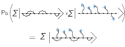
Figure 1: Schematic illustration of a Gutzwiller wavefunction formed from the projected product of a bosonic RVB wavefunction and a Kondo-screened Fermi liquid, to form an entangled combination of both wavefunctions.

This merged wavefunction has, in principle, the potential to capture the two-fluid aspect of the heavy fermion ground-state.

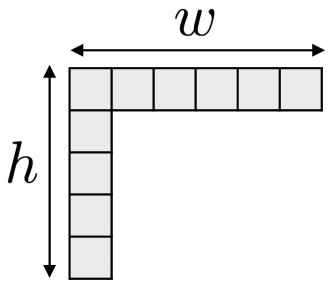
Figure 2: Showing an L-shaped Young tableau, characterized by two parameters, the width $w$ and the height $h$ of the tableau.

I.2 Large-$N$ Approach

The absence of a small parameter in the Kondo model effectively rules out the use of conventional perturbation theory. The alternative approach, followed here, is the use of a large-$N$ expansion in which the fundamental representations contain $N$, rather than $2$ components. In this approach $1/N\sim\hbar_{s}$ plays the role of synthetic Planck’s constant leading to a controlled mean-field (“classical”) theory in the large-$N$ limit, with the possibility of expanding the fluctuations and the constraint condition as a power-series in $1/N$ about the large-$N$ limit. The simplest generalization takes $SU(2)$ to $SU(N)$readnewns ; coleman ; auerbach ; Col6 ; millis ; Aro . Written in traceless form the $SU(N)$ spin is then

$$S^{SU(N)}_{\alpha\beta} = f_{\alpha}^{\dagger}f_{\beta}+b_{\alpha}^{\dagger}b_{\beta}-\left({n_{F}+n_{B}}\right)\delta_{\alpha\beta}/{N},$$ (8)

where $\alpha,\beta\in\{1,2,...,N\}$. However, in this paper we seek to extend the supersymmetric description of spins to the symplectic subgroup $SP(N)$ of $SU(N)$Rea1 ; Fli1 ; Fli2 :

$$S^{SP(N)}_{\alpha\beta} = f_{\alpha}^{\dagger}f_{\beta}+b_{\alpha}^{\dagger}b_{\beta}-\tilde{\alpha}\tilde{\beta}(f_{-\beta}^{\dagger}f_{-\alpha}+b_{-\beta}^{\dagger}b_{-\alpha}).$$ (9)

Here $N$ must be even, while the range of the elementary spin quantum numbers is $\alpha,\beta\in\{\pm 1,\pm 2,...,\pm N/2\}$. The tilde notation, employed extensively in this article, denotes the sign of the index

$$\tilde{\alpha}\equiv{\rm sgn}(\alpha),$$ (10)

with the analogous definition for other indexes. This new spin operator has the symplectic property $S^{SP(N)}_{\alpha\beta}=-\tilde{\alpha}\tilde{\beta}S^{SP(N)}_{-\beta,-\alpha}$ (and is thus also traceless). The symplectic group $SP(N)$ offers many advantages for condensed matter physics, allowing for a consistent extension of the notion of time reversal symmetry to the large-$N$ limit, which permits one to form singlet pairs of particles that are absent in the $SU(N)$ generalization Fli1 ; Fli2 . This capability is vital to describe antiferromagnetism and superconductivity.

The concept of a supersymmetric spin was introduced in previous studies of impurity Kondo models Gan1 ; Gan2 ; Pep1 ; Col1 . In the work presented here, we follow the lines of Coleman et al.Col1 , with the additional generalization to $SP(N)$, and discuss the spin representations in terms of Young tableaux. Young tableaux provide a precise pictorial rendition of irreducible spin representations: horizontal Young tableaux label completely symmetric representations, which are naturally described by bosons, while vertical Young tableaux label completely antisymmetric representations, usually described by fermions. The use of supersymmetric representations lead us to consider the set of representations characterized by L-shaped Young tableaux (Fig. 2). These representations are characterized by two constants:

1. the total number of elementary spins (or boxes) in the representation $Q=h+w-1$, where $h$ and $w$ are height, and width of the Young tableau, respectively, and

2. the asymmetry $Y=h-w$ of the L-shaped Young tableau, as discussed in Coleman et al.Col1 .

The asymmetry of the representation is absent in a physical $SU(2)$ spin-1/2, in which case the Young tableau is depicted by a single box, but once we enlarge the symmetry group of the spin in order to develop a large-$N$ theory, we find a family of representations that range from a completely symmetric representation, fully described by bosons, to a completely antisymmetric representation, described only by fermions, including a whole plethora of intermediate representations that we refer to as mixed representations, depicted by L-shaped Young tableaux (see Fig. 3). The possibility of mean-field solutions described by mixed representations is interesting as it may permit the description of new states of matter, including coexistence of magnetism with superconductivity or with heavy Fermi liquid phases.

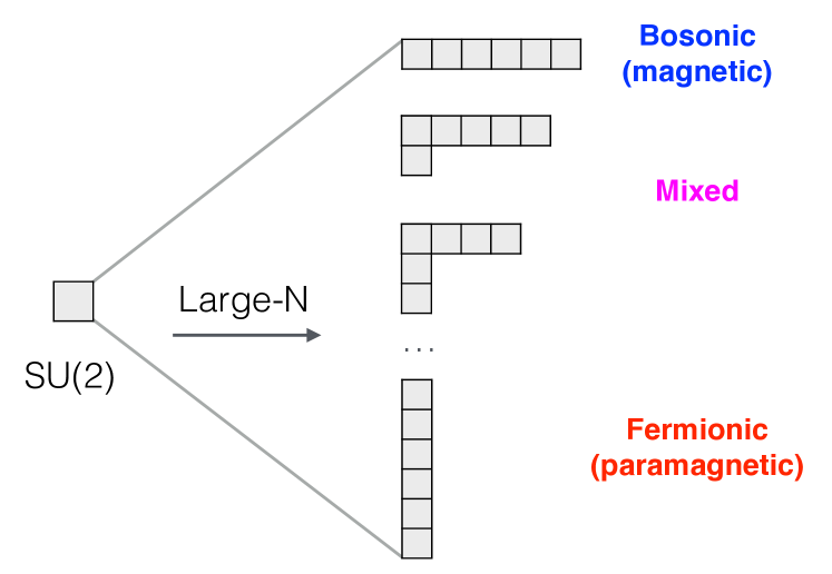
Figure 3: Series of i tableaux in the large-$N$ limit ranging from a fully symmetric (top) towards a fully antisymmetric (bottom), passing through a series of L-shape representations.

For a given value of $N$, one needs to decide which representation to choose in order to proceed with the calculations. Traditionally a purely bosonic representation or a purely fermionic representation is chosen, but the supersymmetric approach provides the possibility of considering an L-shaped representation. To constrain the problem to such a representation one must fix the values of $\hat{Q}=Q_{0}$ and $\hat{Y}=Y_{0}$ through the introduction of projection operators into the partition function:

$$Z=Tr[P_{Q_{0},Y_{0}}e^{-\beta H}].$$ (11)

Typically, the more negative $Y$, the more symmetric the spin representation and the more magnetic the resulting ground-state whereas the more positive $Y$, the more antisymmetric the spin representation and the more Fermi-liquid like the ground-state. To avoid biasing the physics, we consider a grand-canonical ensemble of representations defined by the partition function with indefinite asymmetry $Y$,

$$Z=Tr[P_{Q_{0}}e^{-\beta H}]=\sum_{Y_{0}}Tr[P_{Q_{0},Y_{0}}e^{-\beta H}],$$ (12)

where now we can identify $P_{Q_{0}}$ with the large-$N$ generalization of the Gutzwiller projection operator introduced in Eq. 7:

$$P_{G}\Rightarrow P_{Q_{0}}=\int\Pi_{i}\frac{d\theta_{i}}{2\pi}e^{i\theta_{i}(n_{Bi}+n_{Fi}-Q_{0})}.$$ (13)

This procedure will enable the ensemble to explore the lowest energy configurations. Another motivation to work with the constraint that fixes only the total number of boxes of the representation is the fact that the asymmetry of the representation appears only in the large-$N$ limit, so by letting $Y$ run free provides an unbiased way to take the limit $N\rightarrow 2$, as schematically shown in Fig. 3.

I.3 New features of this work

The large-$N$ limit we now develop places all L-shaped representations with a given number of boxes on the same footing, and the asymmetry of the representation can be thought of as a variational parameter. The character of the representation (bosonic, fermionic or mixed) will now be decided by the energetics of the problem. This will permit us to explore the phase diagram of systems as heavy fermions, in which the character of the spin changes from fermionic in the HFL phase towards bosonic in the AFM region.

Fig. 4 illustrates schematically the evolution of the energy landscape (energy as a function of $q_{F}$, the number of fermions in the representation), for three different values of $T_{K}/T_{RKKY}$. For small $T_{K}/T_{RKKY}$ the energy landscape has a minima for $q_{F}=0$, which means that the system prefers to have a bosonic spin representation and possibly develops magnetic order. Analogously, for large $T_{K}/T_{RKKY}$, the energy landscape has a minimum for the maximum value of $q_{F}$, indicating a purely fermionic representation, which would possibly lead to the development of a heavy Fermi liquid. For intermediate values of $T_{K}/T_{RKKY}$ we find that the representation is mixed, with an energy minima developing at an intermediate value of $q_{F}$ so that the minima is a saddle point as a function of $q_{F}$. We are thus able to identify two classes of solution:

1. Type I minima, in which the free energy is minimized by a purely bosonic or a purely fermionic representation, indicating that the original supersymmetry of the spin is severely broken. In this case the results of a purely bosonic or fermionic representations are recovered;

2. Type II minima, in which mixed representations are energetically favorable. These kinds of minima are candidate representations for a two-fluid picture of heavy fermions. Since the fermionic and bosonic components of the spin fluid acquire the same chemical potential, this opens up the possibility of a new kind of zero mode: a Goldstino, arising from the zero energy cost of rotations between the fermionic and bosonic spin fluid.

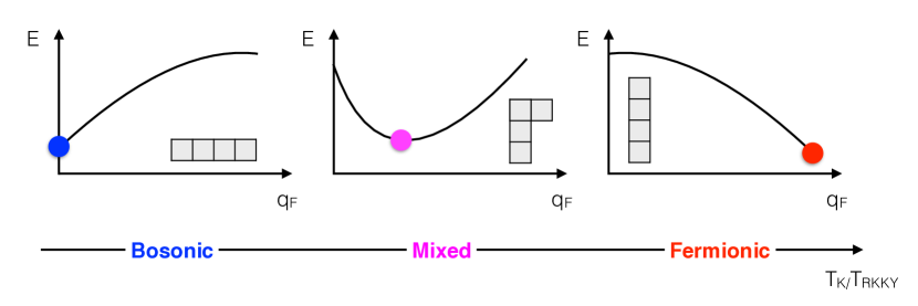
Figure 4: Schematic representation of the evolution of the energy landscape as a function of $q_{F}$ for different values of the ratio $T_{K}/T_{RKKY}$.

Other new features of this work are:

• Symplectic Spins: we generalize the rotation group of the spin from $SU(2)$ to $SP(N)$ for a large-$N$ treatment Fli1 ; Fli2 . This generalization guarantees that all the components of the generalized spin properly invert under time reversal which confers various advantages. In particular, it allows the description of geometrically frustrated magnetismRea1 and it permits the exploration of singlet superconductivity within the large-$N$ framework.

• Spatially inhomogeneous representations: We explore the possibility of solutions which spontaneously develop Kondo, or magnetic character at different sites. Here we are motivated by the partially ordered phase verified experimentally in CePdAl. Fig. 5 represents this kind of solution schematically in a frustrated triangular geometry: one of the local moments in the triangle develops fermionic character, forming a singlet with electrons in the conduction sea, while the other two local moments have a bosonic representation, forming an antiferromagnetic bond.

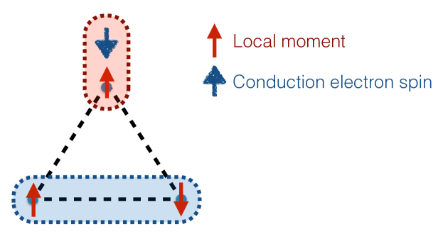
Figure 5: Schematic representation of the inhomogeneous solution for the frustrated triangular geometry.

This paper is organized as follows: in Section II we define the supersymmetric-symplectic spin, identifying the gauge group under which it is invariant and discuss the Casimir for a given irreducible representation. Details on the derivations are given in Appendix A. In Section III we introduce the general path integral formalism which leads to a mean field free energy in the large-$N$ limit. We apply this formalism to a two-impurity model in Section IV, and details on the calculations are given in Appendices B, C and D. In Section V we apply the same formalism to a three-impurity model. We conclude and discuss the open questions in Section VI.

II Supersymmetric-symplectic spins: definitions and properties

We start defining the supersymmetric-symplectic spin:

$$S_{\alpha\beta}=f_{\alpha}^{\dagger}f_{\beta}-\tilde{\alpha}\tilde{\beta}f_{-\beta}^{\dagger}f_{-\alpha}+b_{\alpha}^{\dagger}b_{\beta}-\tilde{\alpha}\tilde{\beta}b_{-\beta}^{\dagger}b_{-\alpha},$$ (14)

where $f_{\alpha}^{\dagger}$, $f_{\alpha}$ and $b_{\alpha}^{\dagger}$, $b_{\alpha}$ are respectively, fermionic and bosonic creation and annihilation operators, with indexes $\alpha,\beta=\{\pm 1,\pm 2,...,\pm N/2\}$, and $\tilde{\alpha}=sgn(\alpha)$, $\tilde{\beta}=sgn(\beta)$. In this form the invertion of the spin under time reversal is made explicit.

We can write the spin operator more concisely as:

$$S_{\alpha\beta}=\Psi^{\dagger}_{\alpha}\gamma_{0}\Psi_{\beta}=\bar{\Psi}_{\alpha}\Psi_{\beta},$$ (15)

by introducing the four component spinor $\bar{\Psi}_{\alpha}=\Psi_{\alpha}^{\dagger}\gamma_{0}$,

$$\Psi_{\alpha}=\left(\begin{array}[]{c}f_{\alpha}\\ \tilde{\alpha}f_{-\alpha}^{\dagger}\\ b_{\alpha}\\ \tilde{\alpha}b_{-\alpha}^{\dagger}\end{array}\right),$$ (20)

which carries the explicit spin index $\alpha$, and has an implicit super-index which runs from 1 to 4 related to the supersymmetric and particle-hole character of its entries; and the matrix

$$\gamma_{0}=\left(\begin{array}[]{cccc}1&0&0&0\\ 0&1&0&0\\ 0&0&1&0\\ 0&0&0&-1\end{array}\right).$$ (25)

We shall follow the convention that super-indices are suppressed and fully contracted with one-another in our formulae, unless otherwise stated.

The supersymmetric-symplectic spin defined in Eq. 15 commutes with the following operator bilinears and the respective conjugates:

$$\hat{n}_{F} =\sum_{\alpha}f_{\alpha}^{\dagger}f_{\alpha},$$

$$\hat{n}_{B} =\sum_{\alpha}b_{\alpha}^{\dagger}b_{\alpha},$$

$$\hat{\psi} =\sum_{\alpha>0}f_{\alpha}f_{-\alpha},$$ (26)

$$\hat{\theta} =\sum_{\alpha}b_{\alpha}^{\dagger}f_{\alpha},$$

$$\hat{\eta} =\sum_{\alpha}\tilde{\alpha}f_{\alpha}b_{-\alpha}.$$

These are therefore generators of the symmetry group of the supersymmetric-symplectic spin. Note that $\hat{\psi}$ and $\hat{\eta}$ are present in the $SP(N)$ but not in the $SU(N)$ generalization of the supersymmetric spin Col1 .

We can rewrite these operators in the form of Hubbard operators Hubbard as follows:

$$X_{00} = \hat{n}_{B},$$ (27)

$$X_{++} = \frac{(\hat{n}_{F}-\hat{n}_{B})}{2},$$ (28)

$$X_{--} = \frac{(N-\hat{n}_{F}-\hat{n}_{B})}{2},$$ (29)

$$X_{+-} = \hat{\psi}^{\dagger},\quad X_{-+}=\hat{\psi},$$ (30)

$$X_{+0} = \frac{\hat{\theta}^{\dagger}}{\sqrt{2}},\quad X_{0+}=\frac{\hat{\theta}}{\sqrt{2}}$$ (31)

$$X_{-0} = \frac{\hat{\eta}}{\sqrt{2}},\quad X_{0-}=\frac{\hat{\eta}^{\dagger}}{\sqrt{2}},$$ (32)

where $X_{00}$, $X_{\pm\pm}$ and $X_{\pm\mp}$ are bosonic Hubbard operators, while $X_{\pm 0}$ and $X_{0\pm}$ are fermionic Hubbard operators. In this form the algebra that these operators follow can be concisely written as:

$$[X_{ab},X_{cd}]_{\pm}=X_{ad}\delta_{bc}\pm X_{cb}\delta_{ad},$$ (33)

where the anticommutator, $(+)$, is used when both Hubbard operators are fermionic, while the commutator, $(-)$, otherwise. The Hubbard algebraHubbard above defines the $SU(2|1)$ supergroupBar . One can explicitly see the $SU(2)$ subgroup generated by the isospin operators

$$\Psi_{1} = (X_{+-}+X_{-+})/2,$$ (34)

$$\Psi_{2} = -i(X_{+-}-X_{-+})/2,$$ (35)

$$\Psi_{3} = (X_{++}-X_{--})/2,$$ (36)

which follow the commutation relation:

$$[\Psi_{i},\Psi_{j}]=i\epsilon_{ijk}\Psi_{k},$$ (37)

and are related to the rotation of the fermionic components of $\Psi_{\alpha}$; while $X_{00}$ defines the generator for the $U(1)$ subgroup associated with the bosons.

Note that one can perform a super-rotation $g$ taking $\Psi_{\alpha}\rightarrow g\Psi_{\alpha}$ which leaves the spin invariant:

$$S_{\alpha\beta}=\Psi^{\dagger}_{\alpha}\gamma_{0}\Psi_{\beta}\rightarrow\Psi^{\dagger}_{\alpha}g^{\dagger}\gamma_{0}g\Psi_{\beta}$$ (38)

if $g$ satisfies

$$g^{\dagger}\gamma_{0}g=\gamma_{0}.$$ (39)

The most general transformation $g$ can be constructed by exponentiation of the generators of the group listed above. An explicit form for g is given in Appendix A.2.

II.1 The Casimir

To uniquely characterize an irreducible representation of $SP(N)$, in principle one needs to define $r=N/2-1$ Casimirs, where $r$ is the rank of the group (the dimension of the Cartan sub-algebra). In terms of Young tableaux, one can understand these parameters as the number of boxes in each row of the tableau (the maximum number of rows in the Young tableau for $SP(N)$ is $N/2$). In this work we restrict our attention to L-shaped tableaux, so we have the extra information that all the rows below the first one have no more than a single box. This reduces the number of parameters required to define the representation to two: $Q$, the total number of boxes, and $Y$, the asymmetry of the representation, as discussed in Coleman et al.Col1 .

From the second Casimir we can identify the quantities $Q$ and $Y$. From NwachukuNwa , we can deduce that for an L-shaped representation in $SP(N)$ the second Casimir can be written in terms of the width $w$ of the first row and the height $h$ of the column in the tableau as:

$$C_{2}=2(w+h)(N+w-h)+4(h-N/2)-2,$$ (40)

and identifying $Q=w+h-1$ and $Y=h-w$, we have

$$C_{2}=2Q(N+1-Y),$$ (41)

the details of this derivation are shown in Appendix A.3.

In terms of operators, the second Casimir can be written as the magnitude of the spin:

$$\mathbf{S}^{2} = \sum_{\alpha\beta}S_{\alpha\beta}S_{\beta\alpha}$$

$$= 2\hat{Q}(N+1-\hat{Y})$$

where:

$$\hat{Q} = \hat{n}_{F}+\hat{n}_{B},$$ (43)

$$\hat{Y} = \hat{n}_{F}-\hat{n}_{B}+1+\frac{4\hat{\psi}^{\dagger}\hat{\psi}-2\hat{\theta}^{\dagger}\hat{\theta}+2\hat{\eta}^{\dagger}\hat{\eta}}{\hat{Q}}.$$ (44)

This form is similar to that found for the $SU(N)$ case (see Appendix A.4 for details of the derivation). Note that in the lowest weight state $|\Psi_{0}\rangle$, where $\psi|\Psi_{0}\rangle=\eta|\Psi_{0}\rangle=\theta|\Psi_{0}\rangle=0$, (corresponding to no pairs and to minimizing the number of fermions) $\mathbf{S}^{2}=2(n_{B}+n_{F})(N-n_{F}+n_{B})$.

We can also write $\mathbf{S}^{2}$ in terms of the $SU(2|1)$ Casimir of the Hubbard operators via the identity:

$$(N^{2}-\mathbf{S}^{2})/4=X_{\alpha\beta}X_{\beta\alpha}-[X_{\alpha 0},X_{0\alpha}]-(X_{00})^{2},$$ (45)

with an implied summation over the repeated indices $\alpha,\beta=\pm$ (See Appendix A.5).

III The formalism

The main topic of interest in our work is the class of Kondo-Heisenberg models involving $SP(N)$ spins, interacting via an additional nearest neighbor antiferromagnetic Heisenberg exchange. These models are written as

$$H=H_{c}+\sum_{j}H_{K}(j)+\sum_{(i,j)}H_{H}(i,j)$$ (46)

where

$$H_{c}=\sum_{{\mathbb{k}}\alpha}\epsilon_{{\mathbb{k}}}c^{\dagger}_{{\mathbb{k}}\alpha}c_{{\mathbb{k}}\alpha}$$ (47)

describes a conduction band of electrons of dispersion $\epsilon_{{\mathbb{k}}}$, where $c^{\dagger}_{{\mathbb{k}}\alpha}$ creates a conduction electron of momentum ${\mathbb{k}}$, spin index $\alpha\in\{\pm 1,\pm 2,...,\pm N/2\}$. The term

$$H_{K}(j)=\frac{J_{K}}{N}\sum_{\alpha\beta}S_{\alpha\beta}(j)s_{\beta\alpha}(j)$$ (48)

describes the Kondo interaction at site $j$, where $S_{\alpha\beta}(j)=\bar{\Psi}_{j\alpha}\Psi_{j\beta}$ defines the local moment operator as in Eq. 15 and the conduction electron spin operators are also written in symplectic form:

$$s_{\alpha\beta}(j)=c_{j\alpha}^{\dagger}c_{j\beta}-\tilde{\alpha}\tilde{\beta}c_{j-\beta}^{\dagger}c_{j-\alpha}.$$ (49)

The final term describes the Heisenberg interaction between spins at sites $i$ and $j$, given by

$$H_{H}(i,j)=\frac{J_{H}}{N}\sum_{\alpha\beta}S_{\alpha\beta}(i)S_{\beta\alpha}(j).$$ (50)

To display the supersymmetric gauge character of the interactions we now rearrange the order of the operators. First, using the properties of the symplectic spin, $\tilde{\alpha}\tilde{\beta}S_{\alpha\beta}=-S_{-\beta,-\alpha}$, the two parts of the electron spin operator in the Kondo interaction are folded into one as follows:

$$H_{K}(j) = \frac{J_{K}}{N}\sum_{\alpha\beta}S_{\alpha\beta}(j)(c_{j\beta}^{\dagger}c_{j\alpha}-\tilde{\alpha}\tilde{\beta}c_{j-\alpha}^{\dagger}c_{j-\beta})$$ (51)

$$= \frac{2J_{K}}{N}\sum_{\alpha\beta}\bar{\Psi}_{\alpha}(j)\Psi_{\beta}(j)c_{j\beta}^{\dagger}c_{j\alpha}.$$ (52)

Next, we super-commute the $\bar{\Psi}$ field to the right-hand side of the interaction, rewriting the interaction in terms of a supertrace,

$$H_{K}(j)=-\frac{2J_{K}}{N}\sum_{\alpha\beta}{\rm Str}\left[\left(\Psi_{j\beta}c^{\dagger}_{j\beta}\right)\left(c_{j\alpha}\bar{\Psi}_{j\alpha}\right)\right]$$ (53)

where we define the supertrace as ${\rm Str}[A]=A_{11}+A_{22}-A_{33}-A_{44}$ and we have used the property that the dot product of two super-spinors $\bar{\Phi}$ and $\chi$ can be rewritten as a supertrace of their outer-product $[\bar{\Phi}\chi]=-{\rm Str}[\chi\bar{\Phi}]$. Notice that ${\nu}_{j}=\left(\Psi_{j\alpha}c^{\dagger}_{j\alpha}\right)$ and $\bar{\nu}_{j}=\left(c_{j\beta}\bar{\Psi}_{j\beta}\right)$ are four component column and row spinors that respectively transform like $\Psi_{j\alpha}$ and $\bar{\Psi}_{j\alpha}$ under super-rotations.

In a similar fashion, we rewrite the Heisenberg interaction as

$$H_{H}(i,j) = \frac{J_{H}}{N}\sum_{\alpha\beta}\bar{\Psi}_{i\alpha}\Psi_{i\beta}\bar{\Psi}_{j\beta}\Psi_{j\alpha}$$ (54)

$$= -\frac{J_{H}}{N}\sum_{\alpha\beta}{\rm Str}\left[\left(\Psi_{i\beta}\bar{\Psi}_{j\beta}\right)\left(\Psi_{j\alpha}\bar{\Psi}_{i\alpha}\right)\right].$$ (55)

Notice that the object $u_{ij}=\left(\Psi_{i\beta}\bar{\Psi}_{j\beta}\right)$ is an outer-product of two super-spinors, forming a four-by-four tensor in superspace that transforms as $u_{ij}\rightarrow g_{i}u_{ij}g_{j}^{-1}$ under super-rotations.

With these manipulations, the Kondo-Heisenberg model can be written as:

$$H=H_{c}-\frac{2J_{K}}{N}\sum_{j,\alpha\beta}{\rm Str}\left[\left(\Psi_{j\alpha}c^{\dagger}_{j\alpha}\right)\left(c_{j\beta}\bar{\Psi}_{j\beta}\right)\right]-\frac{J_{H}}{N}\sum_{(i,j)\alpha,\beta}{\rm Str}\left[\left(\Psi_{i\beta}\bar{\Psi}_{j\beta}\right)\left(\Psi_{j\alpha}\bar{\Psi}_{i\alpha}\right)\right].$$ (56)

Notice that the invariance property of the supertrace ${\rm Str}[gTg^{-1}]={\rm Str}[T]$ guarantees that these interactions are gauge-invariant under the local super-rotations $\Psi_{j}\rightarrow g_{j}\Psi_{j}$. The factorized forms of the interactions are convenient for Hubbard-Stratonovich transformations.

The constraint fixing the total number of bosons plus fermions at each site $n_{Fi}+n_{Bi}=Q_{0}$ can also be written in terms of the spinors $\Psi_{i\alpha}$:

$$n_{Fi}+n_{Bi}=\frac{1}{2}\sum_{\alpha}\bar{\Psi}_{i\alpha}\Lambda\Psi_{i\alpha},$$ (57)

where

$$\Lambda=\left(\begin{array}[]{cccc}1&0&0&0\\ 0&-1&0&0\\ 0&0&1&0\\ 0&0&0&-1\end{array}\right).$$ (62)

We can now write the partition function as a functional integral over the constraint field $\lambda$ and the spin carrying boson and fermion fields

$$Z=\int\mathcal{D}\lambda\mathcal{D}\mu e^{-S},$$ (63)

where

$$S=S_{c}+S_{S}+S_{K}+S_{H},$$ (64)

while

$$\mathcal{D}\mu=\mathcal{D}[c,f,b],$$ (65)

is the measure of integration over the canonical $c$, $f$ and $b$ fields and

$${\cal D}\lambda=\prod_{j}d\lambda_{j}$$ (66)

is the measure of integration over the constraint.

The components of the action are:

$$S_{c}=\int_{0}^{\beta}d\tau\sum_{{\mathbb{k}}\alpha}c^{\dagger}_{{\mathbb{k}}\alpha}(\partial_{\tau}+\epsilon_{{\mathbb{k}}})c_{{\mathbb{k}}\alpha},$$ (67)

the conduction electron part of the action;

$$S_{S}=\!\!\int_{0}^{\beta}\!\!d\tau\left[\frac{1}{2}\sum_{j,\alpha}\bar{\Psi}_{j\alpha}(\partial_{\tau}+\lambda_{j}\Lambda)\Psi_{j\alpha}-\sum_{j}\lambda_{j}Q_{0}\right]$$ (68)

describes the Berry phase, with the constraint $n_{Bj}+n_{Fj}=Q_{0}$ imposed via the introduction of the Lagrange multiplier $\lambda_{j}$ at each site, while

$$S_{K} = \int_{0}^{\beta}d\tau\sum_{j}H_{K}(j),$$ (69)

$$S_{H} = \int_{0}^{\beta}d\tau\sum_{(ij)}H_{H}(i,j)$$ (70)

are the Kondo and Heisenberg parts of the action.

Inside the path integral, we can now carry out a Hubbard-Stratonovich transformation of the interactions. The Kondo part of the interaction is factorized as follows

$$H_{K}(j) = -\frac{2J_{K}}{N}\sum_{\alpha\beta}{\rm Str}\left[\left(\Psi_{j\alpha}c^{\dagger}_{j\alpha}\right)\left(c_{j\beta}\bar{\Psi}_{j\beta}\right)\right]\rightarrow$$ (71)

$$H_{K}^{\prime}(j) = \sum_{\alpha}{\rm Str}\left[\left(\Psi_{j\alpha}c^{\dagger}_{j\alpha}\right)\bar{V}_{j}+V_{j}\left(c_{j\alpha}\bar{\Psi}_{j\alpha}\right)+\frac{N}{2J_{K}}\bar{V}_{j}V_{j}\right]$$ (72)

$$= \sum_{\alpha}\left[\left(\bar{V}_{j}\Psi_{j\alpha}\right)c^{\dagger}_{j\alpha}+c_{j\alpha}\left(\bar{\Psi}_{j\alpha}V_{j}\right)\right]+\frac{N}{2J_{K}}Tr[V_{j}\bar{V}_{j}].$$ (73)

In the last step we have absorbed the minus sign associated with the anticommutation of $c^{\dagger}_{j\alpha}$ and $\left(\bar{V}_{j}\Psi_{j\alpha}\right)$, likewise $c_{j\alpha}$ and $\left(\bar{\Psi}_{j\alpha}V_{j}\right)$. These Hubbard-Stratonovich fields $V_{j}$ and $\bar{V}_{j}=V^{\dagger}_{j}\gamma_{0}$ are four-component spinors

$$V_{j}=\left(\begin{array}[]{c}v_{j}\\ {d}_{j}\\ \phi_{j}\\ {\xi}_{j}\end{array}\right),\qquad\bar{V}_{j}=(\bar{v}_{j},\bar{d}_{j},\bar{\phi}_{j},-\bar{\xi}_{j}).$$ (78)

Here $v_{i}$ and $d_{i}$ are complex fields related to the hybridization between f-fermions and c-electrons and the development of superconductivity by the formation of pairs between f-fermions and c-electrons, respectively. The parameters $\phi_{i}$ and $\xi_{i}$ are complex Grassmann numbers, the first related to the hybridization between b-bosons and c-electrons and the second related to the development os pairs formed between b-bosons and c-fermions.

In a similar fashion, the Heisenberg term decouples as:

$$H_{H}(i,j)\rightarrow H_{H}^{\prime}(i,j) = -\sum_{\alpha}{\rm Str}\left[\Delta_{ij}\left(\Psi_{j\alpha}\bar{\Psi}_{i\alpha}\right)+\left(\Psi_{i\alpha}\bar{\Psi}_{j\alpha}\right)\bar{\Delta}_{ij}\right]+\frac{N}{J_{H}}{\rm Str}\left[\bar{\Delta}_{ij}\Delta_{ij}\right]$$ (79)

$$= \sum_{\alpha}\left[\bar{\Psi}_{i\alpha}\Delta_{ij}\Psi_{j\alpha}+\bar{\Psi}_{j\alpha}\bar{\Delta}_{ij}\Psi_{i\alpha}\right]+\frac{N}{J_{H}}{\rm Str}\left[\bar{\Delta}_{ij}\Delta_{ij}\right]$$ (80)

where $\Delta_{ij}$ is a four-by-four matrix and its conjugate is defined as $\bar{\Delta}_{ij}=\gamma_{0}\Delta_{ij}^{\dagger}\gamma_{0}$. The structure of the matrix is as follows

$$\Delta_{ij}=\left(\begin{array}[]{cc}\Delta_{F}&\tilde{\Delta}_{S}\\ {\Delta}_{S}&\Delta_{B}\end{array}\right)_{ij},$$ (83)

where the diagonal block-matrices composed by c-numbers whereas the off-diagonal block matrices $\Delta_{S}$ and $\tilde{\Delta}_{S}$ are composed by Grassmanians. The internal structure of these blocks is given by

$$(\Delta_{F})_{ij}=\left(\begin{array}[]{cc}t_{ij}&p_{ij}\\ \bar{p}_{ij}&-\bar{t}_{ij}\end{array}\right),$$ (86)

$$(\Delta_{B})_{ij}=\left(\begin{array}[]{cc}q_{ij}&g_{ij}\\ \bar{g}_{ij}&-{\bar{q}}_{ij}\end{array}\right),$$ (89)

$$(\Delta_{S})_{ij}=\left(\begin{array}[]{cc}\gamma_{ij}&\mu_{ij}\\ -\bar{\mu}_{ij}&\bar{\gamma}_{ij}\\ \end{array}\right),$$ (92)

where the remaining matrix is defined through the relation $(\tilde{\Delta}_{S})_{ij}=\sigma_{3}(\Delta_{S})_{ji}$. The matrix $\Delta_{ij}$ can be thought of as supersymmetric RVB field. The components fields $t_{ij}$ and $p_{ij}$ promote hopping and pairing amongst the f-fermions in different sites and the complex fields $q_{ij}$ and $g_{ij}$ promote hopping and magnetic bond formation between the b-bosons. The Grassmannian parameters $\gamma_{ij}$ are hopping amplitudes that transmute bosons into fermions and vice versa, while the Grassmannian amplitudes $\mu_{ij}$ describe pairing between bosons and fermions at different sites.

The partition function now reads:

$$Z=\int{\cal D}[\lambda,V,\Delta]{\cal D}\mu e^{-S^{\prime}},$$ (93)

where

$$S^{\prime}=S_{c}+S_{S}+S^{\prime}_{K}+S^{\prime}_{H},$$ (94)

where the primes denote the actions of the Hubbard-Stratonovich factorized interactions

$$S^{\prime}_{K} = \int_{0}^{\beta}d\tau\sum_{j}H^{\prime}_{K}(j),$$ (95)

$$S^{\prime}_{J} = \int_{0}^{\beta}d\tau\sum_{\langle i,j\rangle}H^{\prime}_{H}(i,j),$$ (96)

and the integral over $\mathcal{D}[V,\Delta]$ indicates the integral over all the fluctuating fields introduced by the Hubbard-Stratonovich transformations. Here c-number fields are represented by the latin letters $(v,d,p,t,q,g)$, while the Grassmannian fields are represented by the Greek letters $(\phi,\xi,\gamma,\mu)$. Grassmannian fields are introduced in order to decouple terms with fermionic bilinears. Note that the Kondo and Heisenberg parts of the action are invariant under the transformation $\Psi_{j\sigma}\rightarrow g_{j}\Psi_{{j}\sigma}$ if the fluctuating field matrices transform accordingly as

$$V_{j} \rightarrow g_{j}V_{j}$$ (97)

$$\Delta_{ij} \rightarrow g_{i}\Delta_{ij}g_{j}^{-1}.$$ (98)

Now we move to the discussion of the implementation of the constraint by fixing $\hat{Q}=Q_{0}$. The constraint can be imposed as a projection operator in each site $j$, written as a delta function:

$$P_{Q_{0}}=\Pi_{j}P_{Q_{0}}^{j}=\Pi_{j}\delta(\hat{Q}_{j}-Q_{0}).$$ (99)

In order to treat the bosonic and fermionic components of the spin in the grand canonical ensemble, we split the constraint into two terms as follows:

$$P_{Q_{0}}^{j}=\sum_{Q_{Fj}=0}^{Q_{0}}\delta(\hat{n}_{Fj}-Q_{Fj})\delta(\hat{n}_{Bj}-Q_{0}+Q_{Fj}).$$ (100)

The constraint fixes the total number of bosons and fermions to $Q_{0}$, leaving the asymmetry of the representation free to adjust according to the energetics of the problem.

This constraint can be implemented in the path integral as a Dirac delta function in its integral form:

$$P_{Q_{0}} = \int\mathcal{D}[Q_{F},\lambda]e^{-\sum_{j}S_{P}(j)},$$ (101)

$$\mathcal{D}[Q_{F},\lambda] = \prod_{j}\sum_{Q_{Fj}}d\lambda_{Fj}d\lambda_{Bj},$$ (102)

where

$$S_{P}(j)=\int_{0}^{\beta}d\tau\biggl{[}\lambda_{Fj}(n_{Fj}-Q_{Fj})+\lambda_{Bj}(n_{Bj}-Q_{0}+Q_{Fj})\biggr{]},$$ (103)

and the constraint fields, $\lambda_{Fj}$ and $\lambda_{Bj}$ are integrated along the imaginary axis. From these considerations $S_{S}$ can be rewritten as:

$$S_{S}\rightarrow S^{\prime}_{S}=\!\!\int_{0}^{\beta}\!\!d\tau\sum_{j}\!\Bigg{(}\sum_{\sigma}\bar{\Psi}_{j\sigma}\frac{(\partial_{\tau}+\Lambda^{\prime}_{j})}{2}\Psi_{j\sigma}-\lambda_{Fj}Q_{Fj}-\lambda_{Bj}(Q_{0}-Q_{Fj})\Bigg{)},$$ (104)

where now

$$\Lambda^{\prime}_{j}=\left(\begin{array}[]{cccc}\lambda_{Fj}&0&0&0\\ 0&-\lambda_{Fj}&0&0\\ 0&0&\lambda_{Bj}&0\\ 0&0&0&-\lambda_{Bj}\end{array}\right),$$ (109)

and the partition function is now written as:

$$Z=\int\mathcal{D}[Q_{F},\lambda,V,\Delta]{\cal D}\mu e^{-S^{\prime}},$$ (110)

where

$$S^{\prime}=S_{c}+S^{\prime}_{S}+S^{\prime}_{K}+S^{\prime}_{H}.$$ (111)

The new feature of this action, is the appearance of the term $Q_{F}$, which tunes the bosonic/fermionic character of the representation. In the large $N$ limit, we will be able to replace the discrete measure of integration over $Q_{F}$ by a continuous measure

$$\sum_{Q_{Fj}}\rightarrow\int_{0}^{Q_{0}}dQ_{Fj}.\qquad(N\rightarrow\infty).$$ (112)

In the large $N$ limit, we anticipate that the functional integral is given by the saddle point value of the effective action, so the large $N$ approximation is then given by the exponential of the effective action

$$Z\approx e^{-S_{eff}[Q_{F},\lambda,V,\Delta]}$$ (113)

where

$$e^{-S_{eff}}=\int{\cal D}[c,f,b]e^{-S^{\prime}}$$ (114)

is the integral over the canonical spin-carrying fermions and bosons in the presence of fixed $Q_{F}$ $\lambda_{B}$, $\lambda_{F}$, $V$ and $\Delta$ with the conditions that $S_{eff}$ be stationary with respect to each of its fields. We may anticipate two classes of mean-field solution

1. Type I solutions, in which the minimum of the effective action occurs at the extremum of the summation over $Q_{Fj}$, i.e $Q_{Fj}=Q_{0}$ or $Q_{Fj}=0$, corresponding to the fully fermionic or bosonic solutions.

2. Type II solutions, in which the minimum of the effective action occurs at some intermediate value of $0<Q_{Fj}<Q_{0}$. Since the action is stationary with respect to variations in $Q_{Fj}$, this implies that

   $$\frac{\delta S_{eff}}{\delta Q_{Fj}}=0=\lambda_{Bj}-\lambda_{Fj}$$ (115)

   so that in this phase, the chemical potential of the bosonic and fermionic spinons are equal,

   $$\lambda_{Bj}=\lambda_{Fj}.$$ (116)

   This equality of chemical potentials allows us to consider these solutions as two fluid solutions.

At the saddle points, we can set all fermionic components of $V$ and $\Delta$ to zero. These terms only contribute to the fluctuations about the mean field theory, so we have

$$V_{j}\rightarrow V_{j}^{0}=\left(\begin{array}[]{c}v_{j}\\ d_{j}\\ 0\\ 0\end{array}\right),$$ (121)

and

$$\Delta_{ij}\rightarrow\Delta_{ij}^{0}=\left(\begin{array}[]{cc}\Delta_{F}&0\\ 0&\Delta_{B}\end{array}\right)_{ij}.$$ (124)

Note that the fermionic and bosonic parts of the action decouple since all the matrices in the action now have the blocks linking the fermionic and bosonic subspaces equal to zero. Now it is possible to solve the fermionic and bosonic problems separately, imposing the constraint $Q_{Fj}+Q_{Bj}=Q_{0}$ to the solution in the end of the calculation. Note that this provides a picture of two asymptotically independent fluids, bosonic and fermionic, in the large-$N$ limit and that the introduction of fluctuations will provide interactions between them.

Now, as a first exploration of this idea we illustrate the formalism with two simple examples: a two-impurity and a frustrated three-impurity model and show that there are stable mean field solutions with mixed representations, as well as with purely bosonic and purely fermionic representations.

IV The Two impurity model

As a first application of the supersymmetric-symplectic spin, we study a minimal model that allows one to make connections to the physics of heavy fermion systems. The model consists of two local moments interacting among themselves by a Heisenberg coupling $J_{H}$ and interacting with its respective bath of conduction electrons by a Kondo coupling $J_{K}$.

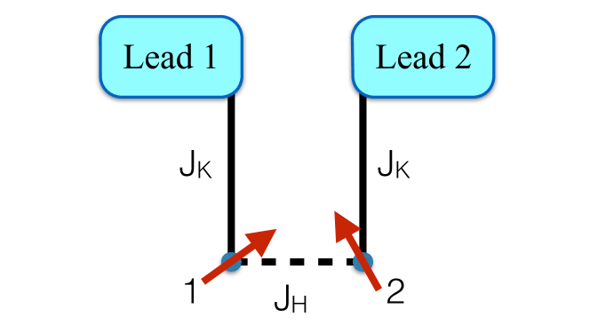
Figure 6: Schematic representation of the two-impurity model.

The Hamiltonian is written as:

$$H=H_{c}+J_{K}\!\sum_{a,\alpha\beta}s_{a\alpha\beta}(0)S_{a\beta\alpha}+J_{H}\!\sum_{\alpha\beta}S_{1\alpha\beta}S_{2\beta\alpha},$$ (125)

where $H_{c}=\sum_{a{\mathbb{k}}\sigma}\epsilon_{{\mathbb{k}}}c_{a{\mathbb{k}}\sigma}^{\dagger}c_{a{\mathbb{k}}\sigma}$ is the conduction electron Hamiltonian, $a=\{1,2\}$ is the lead and local moment index, ${\mathbb{k}}$ the momentum and $\sigma$ the spin index, which assume values $\sigma=\{\pm 1,\pm 2,...,\pm N/2\}$ in the large-N limit. Here $s_{a}(0)$ is the spin density of conduction electrons at the site which is connected to the local moment spin $S_{a}$. Introducing the supersymmetric-symplectic spin, the Hamiltonian can be written in the large-$N$ limit in terms of fermionic and bosonic operators as:

$$H=H_{c} - \frac{2J_{K}}{N}\sum_{a,\alpha\beta}{\rm Str}\left[\left(\Psi_{a\alpha}c^{\dagger}_{a\alpha}\right)\left(c_{a\beta}\bar{\Psi}_{a\beta}\right)\right]$$ (126)

$$- \frac{J_{H}}{N}\sum_{\alpha\beta}{\rm Str}\left[\left(\Psi_{1\beta}\bar{\Psi}_{2\beta}\right)\left(\Psi_{2\alpha}\bar{\Psi}_{1\alpha}\right)\right].$$ (127)

where $\bar{\Psi}_{\sigma}=\Psi_{\sigma}^{\dagger}\gamma_{0}$, as defined in Eq. 20.

We can now apply the formalism introduced in the previous section. We perform a Hubbard-Stratonovich transformation to decouple the interacting terms in the Hamiltonian by introducing fluctuating fields. Within a static mean field solution the fermionic and bosonic problems decouple and are effectively linked only by the constraint; we can now factor the partition function as:

$$Z[q_{F}]=Z_{F}(q_{F})Z_{B}(q_{0}-q_{F}),$$ (128)

where we have defined $q_{0}=Q_{0}/N$, $q_{F}=Q_{F}/N$. We see solutions where the Free energy is minimized with respect to $q_{F}$.

The fermionic part of the partition function reads:

$$Z_{F} = \int\mathcal{D}\mu_{F}e^{-S_{F}},\hskip 14.22636pt\mathcal{D}\mu_{F}=\mathcal{D}[c,f]$$

$$S_{F} =S_{c}+\int_{0}^{\beta}d\tau\sum_{a,\sigma}\left[f^{\dagger}_{a\sigma}(\partial_{\tau}+\lambda_{F})f_{a\sigma}\right.$$ (129)

$$\left.+\sum_{{\mathbb{k}}}\left(f_{a\sigma}^{\dagger}v_{a}c_{a{\mathbb{k}}\sigma}+h.c.\right)\right]$$

$$+\beta N\sum_{a}\frac{|v_{a}|^{2}}{J_{K}}-2\beta N\lambda_{F}q_{F},$$

where we already dropped the terms in $p_{a}$ and $t_{a}$, since it can be shown that these do not contribute to the saddle point solution. Also, the f-operators can be redefined to eliminate the pairing term between c- and f-operators from the Hamiltonian:

$$f_{a\sigma}\rightarrow\tilde{f}_{a\sigma}=\frac{\bar{v}_{a}f_{a\sigma}+d_{a}\tilde{\sigma}f_{a-\sigma}^{\dagger}}{\sqrt{|v_{a}|^{2}+|d_{a}|^{2}}}.$$ (130)

Under these considerations, the fermionic part of the solution reduces to two decoupled impurity problems. Taking $v_{a}=v$ to be site independent, integrating out the conduction electrons in each lead and transforming from imaginary time to Matsubara frequencies (see details in Appendix B):

$$S_{F}=\sum_{na\sigma}f^{\dagger}_{a\sigma}(i\omega_{n})(-i\omega_{n}+\lambda_{F}+i\Gamma_{n})f_{a\sigma}(i\omega_{n})$$

$$\hskip 22.76228pt+2\beta\frac{N|v|^{2}}{J_{K}}-2\beta N\lambda_{F}q_{F},$$ (131)

$$\Gamma_{n}=\Gamma\Theta(D-|i\omega_{n}|)sgn(i\omega_{n}),\hskip 14.22636pt\Gamma=\pi\rho_{0}|v|^{2},$$ (132)

where $\rho_{0}$ is a constant DOS, $D$ is the bandwidth and $\Theta(x)$ is a Heaviside step function. Summing over Matsubara frequencies, in the limit $T\rightarrow 0$, the free energy has the form:

$$\frac{F_{F}}{N} = \frac{2}{\pi}Im\left[\xi_{F}\ln\left(\frac{\xi_{F}}{eT_{K}e^{i\pi q_{F}}}\right)\right],$$ (133)

where we define

$$\xi_{F} = \lambda_{F}+i\Gamma,$$ (134)

and the Kondo temperature

$$T_{K}=De^{-1/\rho_{0}J_{K}}.$$ (135)

In the large-$N$ limit the partition function is dominated by the saddle point. Minimizing the free energy with respect to $\xi_{F}$ one finds

$$\xi_{F}=T_{K}e^{i\pi q_{F}},$$ (136)

and substituting back into the fermionic free energy:

$$\frac{F_{F}}{N}=-\frac{2}{\pi}T_{K}\sin(\pi q_{F}).$$ (137)

The bosonic part of the partition function can be concisely written as:

$$Z_{B} = \int\mathcal{D}\mu_{B}e^{-S_{B}},\hskip 14.22636pt\mathcal{D}\mu_{B}=\mathcal{D}[b,g,\lambda_{B}]$$

$$S_{B} = \int_{0}^{\beta}d\tau\sum_{\sigma}\Psi_{B\sigma}^{\dagger}L_{B}\Psi_{B\sigma}$$ (138)

$$+\beta N\frac{|g|^{2}}{J_{H}}-2\beta N\lambda_{B}(q_{B}+1/2),$$

where

$$L_{B}=\left(\begin{array}[]{cc}\partial_{\tau}+\lambda_{B}&g\\ \bar{g}&-\partial_{\tau}+\lambda_{B}\\ \end{array}\right),$$ (141)

$$\Psi_{B\sigma}=\left(\begin{array}[]{c}b_{1\sigma}\\ \tilde{\sigma}b_{2-\sigma}^{\dagger}\\ \end{array}\right).$$ (144)

Here we already dropped the fluctuating field $q$ since the saddle point solution results in $q=0$. Integrating out the bosons and summing over Matsubara frequencies (see Appendix C), in the zero temperature limit, the free energy is given by:

$$\frac{F_{B}}{N} = \sqrt{\lambda_{B}^{2}-|g|^{2}}+\frac{|g|^{2}}{J_{H}}-2\lambda_{B}(q_{B}+1/2).$$ (145)

Minimizing the free energy with respect to $g$ and $\lambda_{B}$ one finds:

$$\lambda_{B}=J_{H}(q_{B}+1/2),\hskip 28.45274pt|g|^{2}=J_{H}^{2}q_{B}(q_{B}+1),$$ (146)

so the the bosonic free energy can be written as:

$$\frac{F_{B}}{N}=-J_{H}(q_{B}+1/2)^{2},$$ (147)

up to a constant term.

IV.1 Analysis of the free energy

Making explicit use of the constraint condition, $q_{F}+q_{B}=q_{0}$, the total free energy can be written as:

$$\frac{F}{J_{H}N}=-\frac{2}{\pi}A\sin(\pi q_{F})-(q_{0}-q_{F}+1/2)^{2},$$ (148)

where $A=\frac{T_{K}}{J_{H}}$ and the free energy is given in units of $J_{H}$. For each value of $A$ and $q_{0}$ the representation was determined by the minimization of the free energy with respect to $q_{F}$ and the result is plotted in the representation diagram of Fig. 7. In case the free energy is minimized for $q_{F}=q_{0}$ the phase is purely fermionic, meaning that a completely antisymmetric representation is favored. Analogously, for $q_{F}=0$ (or $q_{B}=q_{0}$) the phase is purely bosonic, and a symmetric representation is more appropriate. Solutions with $0<q_{F}<q_{0}$ are solutions in which both bosons and fermions coexist, which we call a mixed phase and label as $(F+B)$ in Fig. 7. Note that for a fixed value of $q_{0}$, as the ratio $T_{K}/J_{H}$ is increased the spins tend to develop fermionic character. Also, for a fixed value of $T_{K}/J_{H}$, increasing $1/q_{0}$ (or reducing $q_{0}$, which is equivalent to decreasing the magnitude of the spin) the spin representation also tends towards a fermionic representation.

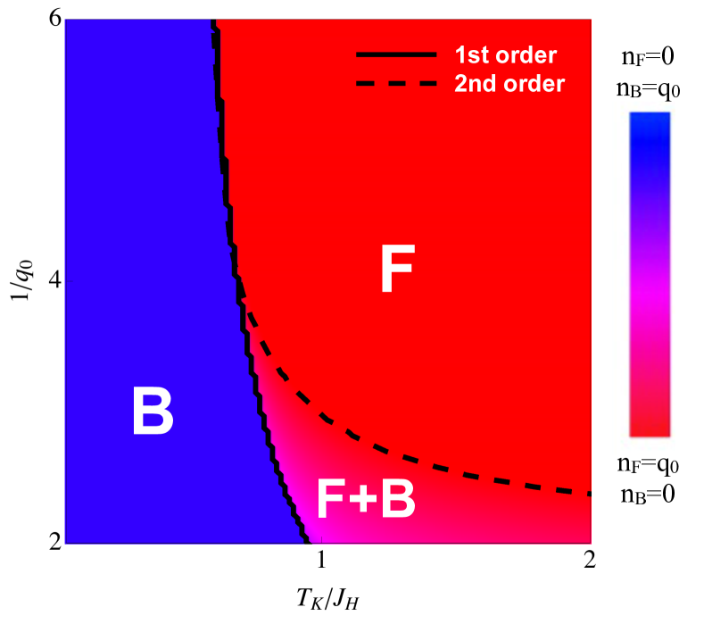
Figure 7: Representation diagram for the two impurity model indicating the most favorable representations as a function of $A=\frac{T_{K}}{J_{H}}$ and $1/q_{0}$. A purely fermionic representation phase (red) is labeled by $F$, a pure bosonic representation phase (blue) is labeled as $B$ and the mixed representation phase (intermediate colors) is labeled by $F+B$.

The dashed line between $F$ and $F+B$ regions indicates a second order phase transition and can be determined from the condition:

$$\left.\frac{\partial F}{\partial q_{F}}\right|_{q_{F}=q_{0}}=0,$$ (149)

which leads to:

$$A=\frac{1}{2\cos(\pi q_{0})}.$$ (150)

The continuous line represents a first order phase transition. The line between the purely fermionic and purely bosonic representations is determined by:

$$\frac{F[q_{F}=q_{0}]}{N}=\frac{F[q_{F}=0]}{N},$$ (151)

which gives the condition:

$$A=\frac{\pi q_{0}(q_{0}+1)}{2\sin(\pi q_{0})}.$$ (152)

The first order line between the phases $B$ and $F+B$ cannot be computed analytically and was determined numerically.

Throughout the mixed phase we have $\lambda_{F}=\lambda_{B}$, so both fluids have the same chemical potential. This is related to the presence of the Type II minima of the free energy (see discussion in the introduction), with a saddle point that allows the coexistence of bosons and fermions and the interchange of one into another at no energy cost. In particular, at the second order “phase transition” line discussed above, when $q_{F}=q_{0}-\delta$ and $q_{B}=\delta$ with $\delta\rightarrow 0$, one can check explicitly from Eq. 146 and 136 that the condition $\lambda_{F}=\lambda_{B}$ gives the same condition that defines the second order line in Eq. 150.

IV.2 Fluctuations of the local fermionic fields

We now analyze the effects of fluctuations of the local fermionic fields. In the previous section we introduced the time dependent fields $\phi_{a}$ and $\xi_{a}$, which allow us to decouple the terms $(b_{a\alpha}c_{a{\mathbb{k}}\alpha}^{\dagger})(c_{a{\mathbb{k}}\beta}b_{a\beta}^{\dagger})$ and $(\tilde{\alpha}b_{a-\alpha}^{\dagger}c_{a{\mathbb{k}}\alpha}^{\dagger})(\tilde{\beta}c_{a{\mathbb{k}}\beta}b_{a-\beta})$ in the action, respectively. These fields do not acquire an expectation value, but fluctuate around zero. The partition function can now be written in terms of the saddle point solution determined in the former subsection times $Z_{\phi}$ and $Z_{\xi}$, the new contributions to the partition function due to the presence of the fluctuating fields $\delta\phi$ and $\delta\xi$, that we take to be site independent. Focusing first in the $\delta\phi$ field:

$$Z_{\phi}\! = \!\int\!D\phi e^{-\int_{0}^{\beta}d\tau\left[\sum_{a{\mathbb{k}}\alpha}(b_{a\alpha}^{\dagger}c_{a{\mathbb{k}}\alpha}\delta\phi+h.c.)+\frac{2N|\delta\phi|^{2}}{J_{K}}\right]}.$$ (153)

Expanding to second order in $\delta\phi$ we can identify the propagator for the fluctuating field $\delta\phi$:

$$[D_{\phi}(i\omega_{r})]^{-1}=2N\left[\chi_{cb}(i\omega_{r})-\frac{1}{J_{K}}\right],$$ (154)

with

$$\chi_{cb}(i\omega_{r}) =$$

$$= -\frac{1}{\beta}\sum_{{\mathbb{k}}{\mathbb{k}}^{\prime}m}G_{b}(i\omega_{r}+i\omega_{m})G_{{\mathbb{k}}{\mathbb{k}}^{\prime}}(i\omega_{m}),$$

where $G_{b}(i\nu_{n})$ is the bosonic propagator and $G_{{\mathbb{k}}{\mathbb{k}}^{\prime}}(i\omega_{n})$ is the full c-electron propagator.

We now evaluate $\chi_{cb}(\omega)$ (details of the calculation can be found in Appendix D). One interesting region for the analysis of $D_{\phi}(i\omega_{r})$ is the second order transition line, where the energy levels of the bosons and fermions are equal. In the infinite bandwidth limit we find:

$$\chi_{cb}(\omega-i\delta)-\frac{1}{J_{K}} = \rho_{0}\omega Re\left[\frac{\log(\lambda+i\Delta)}{\omega+i\Delta}\right]$$ (155)

$$- \frac{\rho_{0}\omega^{2}}{\Delta^{2}+\omega^{2}}\log(\lambda-\omega+i\delta).$$

Note that at zero frequency, $\chi_{cb}(0)-\frac{1}{J_{K}}=0$, so $[D_{\phi}(0)]^{-1}=0$, and the propagator for the fermionic hybridization field $\phi$ diverges at zero frequency at the second order phase transition, indicating the presence of a fermionic zero mode. Also, there is a gap of magnitude equal to $\lambda=\lambda_{F}=\lambda_{B}$ with a continuum that goes up to the bandwidth. This gap is always present in the 2-impurity model since $\lambda=\xi_{B}=J_{H}/2$ is aways finite at the transition. For a Kondo-Heisenberg model in the lattice, the bosonic level will acquire a dispersion and when magnetic order sets in it will be gapless at some points in the Brillouin zone. In that case the spectrum for the fermionic hybridization field is expected to have a continuum of excitations, which can potentially lead to non Fermi liquid behavior.

Figure 8: Plot of the imaginary time of $D(\omega)$, the $\delta\phi$ propagator. The parameters used in this plot were a solution of the mean field theory at a specific point of the second order phase transition: $A=1.57$ and $1/q_{0}=2.5$, which gives $\lambda_{F}=\lambda_{B}=\lambda=1.01$ and $\Delta=2.97$ (in units of $J_{H}$).

For the second fermionic mode $\delta\xi$ a similar calculation follows, where now:

$$[D_{\xi}(i\omega_{r})]^{-1}=2N\left[\bar{\chi}_{cb}(i\omega_{r})-\frac{1}{J_{K}}\right],$$ (156)

with

$$\bar{\chi}_{cb}(i\omega_{r}) =$$

$$= \frac{1}{\beta}\sum_{{\mathbb{k}}{\mathbb{k}}^{\prime}m}G_{b}(i\omega_{r}-i\omega_{m})G_{{\mathbb{k}}{\mathbb{k}}^{\prime}}(i\omega_{m}),$$

and we can write, at the second order transition line:

$$\bar{\chi}_{cb}(\omega-i\delta) - \frac{1}{J_{K}}=\rho_{0}(\omega-2\lambda)Re\left[\frac{\log(-\lambda+i\Delta)}{\omega-2\lambda+i\Delta}\right]$$ (157)

$$- \frac{\rho_{0}(\omega-2\lambda)^{2}}{\Delta^{2}+(\omega-2\lambda)^{2}}\log(\lambda-\omega+i\delta).$$

Here we note that there is no zero mode for this fermionic field at the transition, and a continuum starts at a finite $\lambda=\xi_{B}=J_{H}/2$. This is related to the choice we made to implement the constraint, which is not invariant under all transformations that leave the spin invariant. In particular, it is not invariant under transformations of the form $g_{B}$ (see Appendix A), generated by the operators $\eta^{\dagger}$ and $\eta$.

V Frustration in the three impurity model

As a second application of the supersymmetric-symplectic spin, we study a minimal model that brings in the issue of geometric frustration into play. The model consists of three local moments interacting among themselves by an antiferromagnetic Heisenberg coupling $J_{H}$ and interacting with its respective bath of conduction electrons by a Kondo coupling $J_{K}$, as depicted in Fig. 9. We are motivated to look at this problem by experiments in CePdAl in which the equivalent Ce sites spontaneously develop a state in which one third are paramagnetic and the other two thirds are magnetically ordered Fri2 , exploring the ability of the symplectic representation of the spin to describe frustrated systems.

The Hamiltonian is written as:

$$H=H_{c}+J_{K}\!\sum_{a,\alpha\beta}s_{a\alpha\beta}(0)S_{a\beta\alpha}+J_{H}\!\!\sum_{a,\alpha\beta}\!\!S_{a\alpha\beta}S_{a+1\beta\alpha},$$

where now $a=\{1,2,3\}$ is the lead and local moment index with periodic boundary conditions. As in the previous section, $H_{c}$ is the conduction electron Hamiltonian, $s_{a}(0)$ is the spin density of conduction electrons at the site that is connected to the local moment spin $S_{a}$.

Introducing the supersymmetric-symplectic spin from Eq. 14 into the Hamiltonian, this can be written in the large-$N$ limit as:

$$H = H_{c}-\frac{2J_{K}}{N}\sum_{a,\alpha\beta}{\rm Str}\left[\left(\Psi_{a\alpha}c^{\dagger}_{a\alpha}\right)\left(c_{a\beta}\bar{\Psi}_{a\beta}\right)\right]$$ (159)

$$- \frac{J_{H}}{N}\sum_{a,\alpha\beta}{\rm Str}\left[\left(\Psi_{a\beta}\bar{\Psi}_{a+1\beta}\right)\left(\Psi_{a+1\alpha}\bar{\Psi}_{a\alpha}\right)\right].$$ (160)

with $\Psi_{a\sigma}$ defined in Eq. 20.

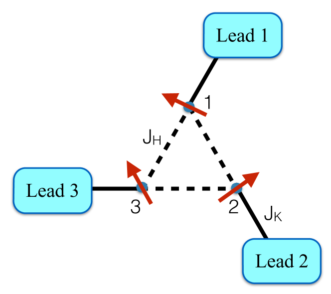
Figure 9: Schematic representation of the frustrated three-impurity model.

Proceeding as in the previous section, within a path integral formalism we introduce fluctuating fields in oder to decouple the quartic terms in the action and impose the constraint by the introduction of a delta function in the integral form. Within a static saddle point solution the problem decouples in to a bosonic and a fermionic part, effectively linked by the constraint. In this section we are going to leave the representation of the spin and the mean field parameters to be determined independently in each site. Omitting the details (similar to the previous section), the partition function in the large $N$ limit can be written as

$$Z=Z_{F}Z_{B},$$ (161)

with the understanding that the partition function is to be stationary with respect to the $q_{Fj}$ at the three sites.

The fermionic part of the partition function can be written as:

$$Z_{F} = \int\mathcal{D}\mu_{F}e^{-S_{F}},\hskip 14.22636pt\mathcal{D}\mu_{F}=\mathcal{D}[c,f]$$

$$S_{F} =S_{c}+\int_{0}^{\beta}d\tau\sum_{a,\sigma}\left[{\bar{f}}_{a\sigma}(\partial_{\tau}+\lambda_{Fa})f_{a\sigma}\right.$$ (162)

$$\left.+\sum_{{\mathbb{k}}}\left(f^{\dagger}_{a\sigma}v_{a}c_{a{\mathbb{k}}\sigma}+h.c.\right)\right]$$

$$+\beta N\sum_{a}\frac{|v_{a}|^{2}}{J_{K}}-\beta N\sum_{a}\lambda_{Fa}q_{Fa},$$

where as in the previous section, we assume that the only fluctuating field that acquires a finite value at the saddle point solution is $v_{a}$. In this case the fermionic part of the solution reduces to three decoupled impurity problems, with the same solution as the previous section, now for 3 leads:

$$\frac{F_{F}}{N}=-\frac{T_{K}}{\pi}\sum_{a}\sin(\pi q_{Fa}).$$ (163)

The bosonic part of the partition function reads:

$$Z_{B} = \int\mathcal{D}[b]e^{-S_{B}},$$ (164)

where

$$S_{B} = \int_{0}^{\beta}d\tau\sum_{\sigma}\Psi_{B\sigma}^{\dagger}\frac{L_{B}}{2}\Psi_{B\sigma}$$ (165)

$$- \frac{\beta N}{2J_{H}}\sum_{a}Tr[\Delta^{\dagger}_{Ba}\gamma_{0}^{B}\Delta_{Ba}\gamma_{0}^{B}]$$

$$- \beta N\sum_{a}\lambda_{Ba}(q_{Ba}+1/2),$$

where we denote $q_{Ba}=q_{0}-q_{Fa}$ and

$$L_{B}=\left(\begin{array}[]{ccc}m_{B1}&\Delta_{B1}&\Delta_{B3}^{\dagger}\\ \Delta_{B1}^{\dagger}&m_{B2}&\Delta_{B2}\\ \Delta_{B3}&\Delta_{B2}^{\dagger}&m_{B3}\end{array}\right),$$ (169)

with

$$m_{Ba}=\left(\begin{array}[]{cc}\partial_{\tau}+\lambda_{Ba}&0\\ 0&-\partial_{\tau}+\lambda_{Ba}\end{array}\right),$$ (172)

$$\Delta_{Ba}=\left(\begin{array}[]{cc}q_{a}&-g_{a}\\ \bar{g}_{a}&{\bar{q}}_{a}\end{array}\right),$$ (175)

and

$$\Psi_{B\sigma}=\left(\begin{array}[]{c}b_{1\sigma}\\ \tilde{\sigma}b_{1-\sigma}^{\dagger}\\ b_{2\sigma}\\ \tilde{\sigma}b_{2-\sigma}^{\dagger}\\ b_{3\sigma}\\ \tilde{\sigma}b_{3-\sigma}^{\dagger}\\ \end{array}\right).$$ (182)

Note that the trace term in the action now appears with a minus sign since it is related to the bosonic part of the super-trace introduced in Eq. 79. Here we define $\gamma_{0}^{B}=\sigma_{3}$ as the bosonic part of the original matrix $\gamma_{0}$.

The solution of the bosonic part of the partition function is more involved if we allow the representations of the spin to be different in each lead. As a first solution we consider the same representation on every site, and look for an homogeneous solution, taking $\lambda_{Ba}\rightarrow\lambda_{B}$, $q_{a}\rightarrow q$ and $g_{a}\rightarrow g$. Integrating out the bosons and summing over Matsubara frequencies, in the zero temperature limit, the free energy can be written as:

$$\frac{F_{B}}{N} = (\lambda_{B}+2q)+2\sqrt{(\lambda_{B}-q)^{2}-3g^{2}}$$ (183)

$$+\frac{3(g^{2}-q^{2})}{J_{H}}-3\lambda_{B}(q_{B}+1/2).$$

Minimizing the free energy with respect to $q$, $g$ and $\lambda_{B}$ one finds the saddle point free energy:

$$\frac{F_{B}}{N}=-\frac{3J_{H}}{2}(q_{B}+1/2)^{2},$$ (184)

up to a constant term. The total free energy for the homogeneous solution can be written, already making explicit use of the constraint condition $q_{F}+q_{B}=q_{0}$, as:

$$\frac{F_{Hom}}{J_{H}N}=-\frac{3}{\pi}A\sin(\pi q_{F})-\frac{3}{2}(q_{0}-q_{F}+1/2)^{2},$$ (185)

where again $A=\frac{T_{K}}{J_{H}}$ and the free energy is given in units of $J_{H}$. Note that this is functionally the same as the 2-impurity model up to an overall factor of $3/2$, and as a consequence the representation diagram determining the most favorable representation for the spin within an homogeneous solution will be identical to the 2-impurity case.

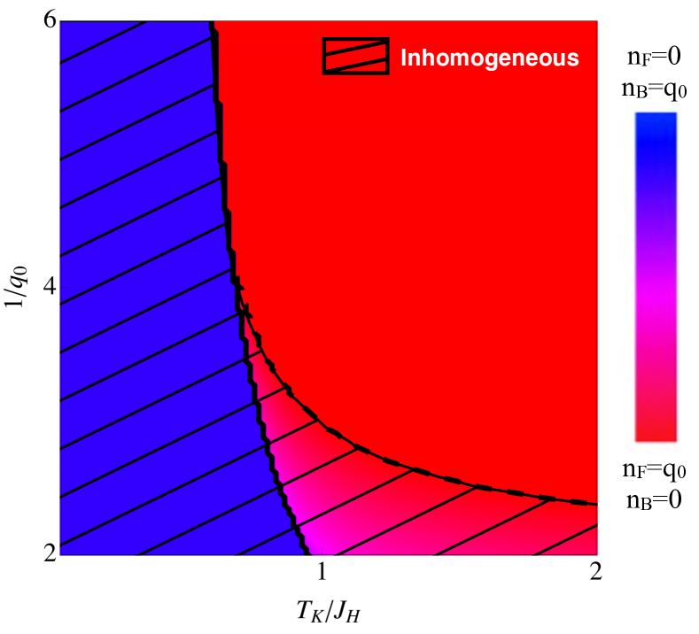
Figure 10: Representation diagram for the three impurity model indicating the most favorable representations as a function of $A=\frac{T_{K}}{J_{H}}$ and $1/q_{0}$. The color code is the same as in Fig. 7. The hashed area represents the region of the diagram in which an inhomogeneous solution is energetically favorable.

Now we move on to investigate solutions which spontaneously develop different representations in each site, which we refer to as inhomogeneous representations. Due to frustration, we expect that it is energetically favorable for one of the spins to be in a fermionic representation, essentially disconnected from the other two spins with a bosonic or mixed representation, forming an antiferromagnetic bond. We assume one of the spins to always have a fermionic representation and let the representation of the two other spins to be selected as the one that minimizes the total energy.

Now the problem reduces to a single impurity problem with a purely fermionic representation plus the two-impurity problem solved in the previous section. The free energy for the inhomogeneous solution reads:

$$\frac{F_{Inh}}{J_{H}N} = -\frac{1}{\pi}A\sin(\pi q_{0})-\frac{2}{\pi}A\sin(\pi q_{F})$$

$$- (q_{0}-q_{F}+1/2)^{2},$$

in units of $J_{H}$, where $A=\frac{T_{K}}{J_{H}}$. Again, the representation diagram will be the same as before, but now we compare the free energies of the homogeneous and inhomogeneous solutions for the 3-impurity problem. The hashed area in Fig. 10 is the region of the diagram in which the inhomogeneous solution is more favorable. This result provides a model for the situation which appears to occur in CePdAl Fri2 : one third of the local moments in the frustrated Kagome lattice (formed by an assembly of corner-shared triangles) relieve the frustration by assuming an antisymmetric character and forming a Kondo singlet with a conduction electron, while the other two thirds of the local moments assume a bosonic character, developing magnetic order, allowing a partially ordered phase to be formed, as depicted in Fig. 5.

VI Conclusion and discussion

In this work we introduced a new supersymmetric-spin representation for large-$N$ treatments, based on a symplectic generalization of the spin operator. We have analyzed the properties of the supersymmetric-symplectic spin and its symmetries, identifying the supergroup $SU(2|1)$ of transformations under which the spin is invariant.

We have proposed a new framework in the large-$N$ limit, which allows the problem to sample different representations, selecting the one which lowers the energy in a given point in parameter space. This opens up the possibility of describing the phase diagram of heavy fermions within a single approach that can capture the evolving character of the spin, at the same time that it offers a potential framework for the phenomenological two-fluid picture for heavy fermions.

Applying this approach to two toy models, the two-impurity model and the frustrated three-impurity model, we have shown two new classes of mean-field theory that may be of interest in developing a unified description of heavy fermion systems. In particular, we find a mixed phase solution in which bosons and fermion coexist at each site, which points the way to a description of the coexistence of magnetism and Kondo effect. Also, we find stable inhomogenous solutions, which may provide a basis for describing the partially ordered state in CePdAl CePdAl1 ; CePdAl2 ; Fri2 .

There are many open questions raised by our work. Firstly, within the mixed phase, we find evidence for a new kind of zero mode, a Goldstino, that results from the partial breaking of supersymmetry. This can be understood as a consequence of the fact that the Hamiltonian is invariant under super-rotations while at the same time, the mean-field solution breaks this rotational symmetry. Given a state $|\Psi\rangle$ with a fermion assigned to the corner box, for example, one can rotate this state as follows:

$$|\Psi\rangle\rightarrow\theta^{\dagger}_{j}|\Psi\rangle=f^{\dagger}_{j\sigma}b_{j\sigma}|\Psi\rangle,$$ (187)

and find a new state which has same energy. These kinds of zero modes are only present when the chemical potential of the bosons and fermions are equal, i.e in type II solutions. We note that in the presence of a Kondo effect, the f-electrons are charged, whereas b-bosons are neutral, so the fermionic Goldstino excitation is charged and may represent a zero energy valence fluctuation. Further work is needed to establish whether such zero modes are a truly physical excitation and whether they participate in anomalous inelastic scattering and the development of non-Fermi liquid behavior.

Secondly, we would like to discuss the future application of this approach to the exploration of the phase diagram of the Kondo lattice. Extrapolating the results found in this work to the lattice we expect to find that for small ratios of $T_{K}/J_{H}$ a bosonic representation is more favorable in which magnetic order will emerge once the bosons condense. Heavy Fermi liquid behavior is expected to develop when there are fermions in the representation, which can hybridize with the conduction electrons. If a mixed phase is stable in the lattice, heavy fermion behavior can coexist with magnetic order. In principle, this approach allows us to explore the different kinds of phase transitions as seen in YbRh₂Si₂Pas ; Geg2 ; Fri1 within a single approach: given that the fermions now can form a Fermi surface, the magnetic phase can emerge both from local moments within the bosonic representation or as an instability of the large Fermi surface. Another aspect of interest is the possibility of the description of superconductivity; this phase is likely to develop in the mixed phase and its vicinity, as a consequence of a valence-bond kind of magnetism emerging from the fermionic antiferromagnetic bonds. This is another interesting direction for future work.

Acknowledgments. The authors thank Catherine Pépin, Onur Erten and Tzen Ong for fruitful discussions and the Kavli Institute for Theoretical Physics for hosting the authors during the Fall 2014 where part of this work was completed. This research was supported in part by the National Science Foundation under Grant No. NSF PHY11-25915 and NSF DMR-1309929 and by a Simons Foundation fellowship (PC).

Appendix A Details on the properties of supersymmetric symplectic spin

In this appendix we discuss a few properties of the supersymmetric symplectic spin in more detail.

A.1 Number of spin components

When writing the components of the supersymmetric-symplectic spin as:

$$S_{\alpha\beta}=f_{\alpha}^{\dagger}f_{\beta}-\tilde{\alpha}\tilde{\beta}^{\prime}f_{-\beta}^{\dagger}f_{-\alpha}+b_{\alpha}^{\dagger}b_{\beta}-\tilde{\alpha}\tilde{\beta}^{\prime}b_{-\beta}^{\dagger}b_{-\alpha},$$ (188)

note that we have in fact only $N(N+1)/2$ components (equal to the number of generators of the enlarged symmetry group of the spin, here $SP(N)$). This can be checked by noticing that $S_{\alpha\beta}=-\tilde{\alpha}\tilde{\beta}S_{-\beta-\alpha}$, so the generators are not all independent. For $\alpha,\beta>0$, we have $S_{\alpha\beta}=-S_{-\beta-\alpha}$, so the generators with both indexes negative are linearly dependent on the generators with both indexes positive. For $\alpha>0,\beta<0,\alpha\neq-\beta$ we have $S_{\alpha\beta}=S_{-\beta-\alpha}$, but note that for the case of $\alpha=\beta$ we have the condition $S_{\alpha,-\alpha}=S_{\alpha,-\alpha}$, which does not give a relation between the generators in the off diagonal. One can check that indeed $S_{\alpha,-\alpha}$ is not linearly dependent on $S_{-\alpha,\alpha}$. Within these considerations the number of independent generators is $N(N+1)/2$, as expected.

A.2 Symmetry transformations of the supersymmetric symplectic spin

In the main text, a more concise form of the supersymmetric-symplectic spin is introduced in order to make the local symmetry manifestly clear:

$$S_{\alpha\beta}=\bar{\Psi}^{\dagger}_{\alpha}\Psi_{\beta}=\Psi^{\dagger}_{\alpha}\gamma_{0}\Psi_{\beta},$$ (189)

where,

$$\Psi_{\alpha}=\left(\begin{array}[]{c}f_{\alpha}^{\dagger}\\ \tilde{\alpha}f_{-\sigma}\\ b_{\alpha}^{\dagger}\\ \tilde{\alpha}b_{-\sigma}\end{array}\right)$$ (194)

is a four-component spinor, and as defined in the main text $\gamma_{0}=diag[1,1,1,-1]$, and $\tilde{\alpha}=sgn(\alpha)$.

Under a super-rotation of the spinors $\Psi_{\alpha}\rightarrow g\Psi_{\alpha}$, the spin operator transforms as:

$$S_{\alpha\beta}=\Psi^{\dagger}_{\alpha}\gamma_{0}\Psi_{\beta}\rightarrow\Psi^{\dagger}_{\alpha}g^{\dagger}\gamma_{0}g\Psi_{\beta},$$ (195)

so for the spin to be invariant the transformation $g$ should satisfy:

$$g^{\dagger}\gamma_{0}g=\gamma_{0},$$ (196)

which is essentially the unitarity condition to the transformation after taking appropriate care of the commutativity of the bosons.

The most general transformation $g$ can be obtained by exponentiation of the generators of the algebra introduced in Eq. II. Exponentiation of the even (or commuting) part of the algebra gives:

$$g_{E}=\left(\begin{array}[]{cccc}u&v&0&0\\ -\bar{v}&\bar{u}&0&0\\ 0&0&x&0\\ 0&0&0&\bar{x}\end{array}\right),$$ (201)

where the parameters $u$, $v$ and $x$ are complex numbers satisfying $|u|^{2}+|v|^{2}=1$ and $|x|^{2}=1$. Note the $SU(2)$ and $U(1)$ substructure of this transformation for the fermionic and bosonic parts of the spinor $\Psi_{\sigma}$, respectively.

Exponentiating the odd (or anticommuting) part of the algebra we find:

$$g_{A}=\left(\begin{array}[]{cccc}1+\frac{\alpha\bar{\alpha}}{2}&0&-\bar{\alpha}&0\\ 0&1+\frac{\alpha\bar{\alpha}}{2}&0&-\alpha\\ \alpha&0&1-\frac{\alpha\bar{\alpha}}{2}&0\\ 0&-\bar{\alpha}&0&1-\frac{\alpha\bar{\alpha}}{2}\end{array}\right),$$ (206)

and

$$g_{B}=\left(\begin{array}[]{cccc}1-\frac{\beta\bar{\beta}}{2}&0&0&-\bar{\beta}\\ 0&1-\frac{\beta\bar{\beta}}{2}&\beta&0\\ 0&-\bar{\beta}&1+\frac{\beta\bar{\beta}}{2}&0\\ -\beta&0&0&1+\frac{\beta\bar{\beta}}{2}\end{array}\right),$$ (211)

where the parameters $\alpha$ and $\beta$ are complex Grassmann numbers.

The most general transformation can be obtained by the composition of the three transformations above:

$$g=g_{E}g_{A}g_{B},$$ (212)

which satisfies the condition $g^{\dagger}\gamma_{0}g=\gamma_{0}$, as required.

A.3 Derivation of the Casimir

We now follow NwachukuNwa in order to derive the second Casimir of $SP(N)$, (where $N$ is an even number), given in Eq. 40. Each irreducible representation of $SP(N)$ is characterized by the set of integers $(f_{N/2},f_{N/2-1},...,f_{1})$. This set of numbers corresponds to the number of boxes in each row of the respective Young tableau, starting from the topmost and longest row, which has $f_{N/2}$ boxes. These numbers also correspond to the eigenvalues of the $N/2$ Cartan (diagonal) generators in the highest state of the representation. Following Nwa , if we define:

$$\lambda_{i}=f_{i}+N/2+i,\hskip 14.22636pt\text{for $i\geq 0$}$$ (213)

$$\lambda_{-i}=-\lambda_{i}+N,\hskip 14.22636pt\text{for $i>0$}$$ (214)

$$\rho_{i}=N/2+i,$$ (215)

where we take $f_{0}=0$, the second Casimir is written:

$$C_{2}=\sum_{i=-N/2}^{N/2}(\lambda_{i}^{2}-\rho_{i}^{2}).$$ (216)

For an L-shaped tableau with width $w$ and height $h$, we have:

$$f_{i}=\begin{cases}w,&\text{$i=\frac{N}{2}$},\\ 1,&\text{$\frac{N}{2}-1\geq i\geq\frac{N}{2}-h+1$},\\ 0,&\text{$i\leq\frac{N}{2}-h$},\end{cases}$$ (217)

therefore:

$$\lambda_{i}=\begin{cases}w+N,&\text{$i=\frac{N}{2}$},\\ -w,&\text{$i=-\frac{N}{2}$},\\ 1+N/2+i,&\text{$\frac{N}{2}-1\geq i\geq\frac{N}{2}-h+1$},\\ -1+N/2+i,&\text{$-|\frac{N}{2}-1|\leq i\leq-|\frac{N}{2}-h+1|$},\\ 0,&\text{otherwise},\end{cases}$$ (218)

and

$$\rho_{i}=\begin{cases}N,&\text{$i=\frac{N}{2}$},\\ 0,&\text{$i=-\frac{N}{2}$},\\ N/2+i,&\text{$\frac{N}{2}-1\geq i\geq\frac{N}{2}-h+1$},\\ N/2+i,&\text{$-|\frac{N}{2}-1|\leq i\leq-|\frac{N}{2}-h+1|$},\\ 0,&\text{otherwise},\end{cases}$$ (219)

so we can perform the sum:

$$C_{2} = w^{2}+4Nw+w^{2}$$

$$+ \sum_{i=N/2-h+1}^{N/2-1}(1+N+2i)$$

$$+ \sum_{i=-N/2+1}^{-N/2+h-1}(1-N-2i),$$

$$= 2(w+h)(N+w-h)+4(h-N/2)-2,$$

where the sums were evaluated as sums of arithmetic progressions. This is Eq. 40 in the main text. Identifying $Q=w+h-1$ and $Y=h-w$, we have

$$C_{2} = 2(Q+1)(N-Y)+2(Y+Q+1-N)-2$$ (221)

$$= 2(Q+1)(N-Y)-2N+2(Y+Q)$$ (222)

$$= 2Q(N+1-Y),$$ (223)

which is Eq. 41, similar to the form discussed in Coleman et al.Col1 in the case of an SU(N) generalization of the supersymmetric spin.

A.4 Operator form of the Casimir

Now we relate the magnitude of the spin $\mathbf{S}^{2}$ with the Casimir computed above. We start computing:

$$\mathbf{S}^{2} = \sum_{\alpha\beta}S_{\alpha\beta}S_{\beta\alpha},$$ (224)

with $S_{\alpha\beta}$ is defined in Eq. 14. Taking the operator products and relabeling the summed indexes we find:

$$\mathbf{S}^{2} = 2(f_{\alpha}^{\dagger}f_{\beta}f_{\beta}^{\dagger}f_{\alpha}+b_{\alpha}^{\dagger}b_{\beta}b_{\beta}^{\dagger}b_{\alpha}+2f_{\alpha}^{\dagger}f_{\beta}b_{\beta}^{\dagger}b_{\alpha}$$ (225)

$$- \tilde{\alpha}\tilde{\beta}f_{\alpha}^{\dagger}f_{\beta}f_{-\alpha}^{\dagger}f_{-\beta}-\tilde{\alpha}\tilde{\beta}b_{\alpha}^{\dagger}b_{\beta}b_{-\alpha}^{\dagger}b_{-\beta}-2\tilde{\alpha}\tilde{\beta}f_{\alpha}^{\dagger}f_{\beta}b_{-\alpha}^{\dagger}b_{-\beta}),$$ (226)

where we have used summation convention for the repeated spin indices. The first line of this expression is the Casimir for the $SU(N)$ spin, while the second line introduces the additional cross-terms that result from the symplectic form of the spin.

Expanding the first line, we have

$$f^{\dagger}_{\alpha}f_{\beta}f^{\dagger}_{\beta}f_{\alpha} = n_{F}(N-n_{F})+n_{F}$$ (227)

$$b^{\dagger}_{\alpha}b_{\beta}b^{\dagger}_{\beta}b_{\alpha} = n_{B}(N+n_{B})-n_{B}$$ (228)

$$f^{\dagger}_{\alpha}f_{\beta}b^{\dagger}_{\beta}b_{\alpha} = \theta^{\dagger}\theta-n_{F}$$ (229)

so that

$$f_{\alpha}^{\dagger}f_{\beta}f_{\beta}^{\dagger}f_{\alpha}+b_{\alpha}^{\dagger}b_{\beta}b_{\beta}^{\dagger}b_{\alpha}+2f_{\alpha}^{\dagger}f_{\beta}b_{\beta}^{\dagger}b_{\alpha}=(n_{B}+n_{F})(N+n_{B}-n_{F})+2\theta^{\dagger}\theta-(n_{B}+n_{F})$$ (230)

Now expanding the additional cross terms,

$$-\tilde{\alpha}\tilde{\beta}f_{\alpha}^{\dagger}f_{\beta}f_{-\alpha}^{\dagger}f_{-\beta} = n_{F}-\tilde{\alpha}\tilde{\beta}f^{\dagger}_{\alpha}f^{\dagger}_{-\alpha}f_{-\beta}f_{\beta}=n_{F}-4\psi^{\dagger}\psi,$$ (231)

$$-\tilde{\alpha}\tilde{\beta}b_{\alpha}^{\dagger}b_{\beta}b_{-\alpha}^{\dagger}b_{-\beta} = n_{B}-\tilde{\alpha}\tilde{\beta}b_{\alpha}^{\dagger}b_{-\alpha}^{\dagger}b_{-\beta}b_{\beta}=n_{B},$$ (232)

$$-2\tilde{\alpha}\tilde{\beta}f_{\alpha}^{\dagger}f_{\beta}b_{-\alpha}^{\dagger}b_{-\beta} = -2\tilde{\alpha}\tilde{\beta}f^{\dagger}_{\alpha}b^{\dagger}_{-\alpha}b_{-\beta}f_{\beta}=-2\eta^{\dagger}\eta$$ (233)

where we have used the fact that the bosonic pairs vanish $\sum_{\beta}\tilde{\beta}b_{-\beta}b_{\beta}=0$. Combining the additional cross terms, we have

$$-\tilde{\alpha}\tilde{\beta}f_{\alpha}^{\dagger}f_{\beta}f_{-\alpha}^{\dagger}f_{-\beta}-\tilde{\alpha}\tilde{\beta}b_{\alpha}^{\dagger}b_{\beta}b_{-\alpha}^{\dagger}b_{-\beta}-2\tilde{\alpha}\tilde{\beta}f_{\alpha}^{\dagger}f_{\beta}b_{-\alpha}^{\dagger}b_{-\beta})=n_{F}+n_{B}-4\psi^{\dagger}\psi-2\eta^{\dagger}\eta.$$ (234)

Combining (230) and (234), noting that the remainder terms $\pm(n_{B}+n_{F})$ cancel one-another, we obtain

$$\mathbf{S}^{2} = 2\left[(\hat{n}_{B}+\hat{n}_{F})(N+\hat{n}_{B}-\hat{n}_{F})-4\hat{\psi}^{\dagger}\hat{\psi}+2\hat{\theta}^{\dagger}\hat{\theta}-2\hat{\eta}^{\dagger}\hat{\eta}\right],$$ (235)

so we can identify:

$$\mathbf{S}^{2} = 2\hat{Q}(N+1-\hat{Y}),$$ (236)

where

$$\hat{Q} = \hat{n}_{F}+\hat{n}_{B},$$ (237)

$$\hat{Y} = \hat{n}_{F}-\hat{n}_{B}+1+\frac{4\hat{\psi}^{\dagger}\hat{\psi}-2\hat{\theta}^{\dagger}\hat{\theta}+2\hat{\eta}^{\dagger}\hat{\eta}}{\hat{Q}}.$$ (238)

A.5 Sum rule for spin and super-Casimir

The second Casimir invariant $\chi^{2}$ of the $SU(2|1)$ group can be written hopkinson

$$\chi^{2}={\rm Tr}[XmX],$$ (239)

where $X\equiv X_{ab}$ is the three-dimensional matrix formed out of the Hubbard operators and $m={\rm diag}(1,1,-1)$. If we expand this result we obtain

$$\chi^{2}=X_{\alpha\beta}X_{\beta\alpha}-[X_{\alpha 0},X_{0\alpha}]-(X_{00})^{2},$$ (240)

with an implied summation over the repeated indices $\alpha,\beta=\pm$. Substituting for the Hubbard operators using (27) we obtain

$$\chi^{2} = X_{++}^{2}+X_{--}^{2}-X_{00}^{2}+\{X_{+-},X_{-+}\}-[X_{+0},X_{0+}]-[X_{-0},X_{0-}]$$ (241)

$$= [(n_{F}-n_{B})/2]^{2}+[(N-n_{F}-n_{B})/2]^{2}-\hat{n}_{B}^{2}+\{\hat{\psi}^{\dagger},\hat{\psi}\}-[\hat{\theta}^{\dagger},\hat{\theta}]/2-[\hat{\eta},\hat{\eta}^{\dagger}]/2$$ (242)

$$= N^{2}/4-(n_{F}+n_{B})(N-n_{F}+n_{B})/2+\{\psi^{\dagger},\psi\}-[\theta^{\dagger},\theta]/2+[\eta^{\dagger},\eta]/2.$$ (243)

Using the Hubbard algebra of the $SU(2|1)$ generators (33), we have

$$\{\psi^{\dagger},\psi\} = 2\psi^{\dagger}\psi+[\psi,\psi^{\dagger}]=2\psi^{\dagger}\psi+[X_{-+},X_{+-}]=2\psi^{\dagger}\psi+X_{--}-X_{++},$$ (244)

$$[\theta^{\dagger},\theta]/2 = \theta^{\dagger}\theta-\{\theta,\theta^{\dagger}\}/2=\theta^{\dagger}\theta-\{X_{0+},X_{+0}\}=\theta^{\dagger}\theta-(X_{00}+X_{++}),$$ (245)

$$[\eta^{\dagger},\eta]/2 = \eta^{\dagger}\eta-\{\eta,\eta^{\dagger}\}=\eta^{\dagger}\eta-\{X_{-0},X_{0-}\}=\eta^{\dagger}\eta-(X_{--}+X_{00}),$$ (246)

Adding up these expressions, we find that

$$\{\psi^{\dagger},\psi\}-[\theta^{\dagger},\theta]/2+[\eta^{\dagger},\eta]/2=2\psi^{\dagger}\psi-\theta^{\dagger}\theta+\eta^{\dagger}\eta.$$ (247)

Inserting this into (241) we obtain

$$\chi^{2}=N^{2}/4-(n_{F}+n_{B})(N-n_{F}+n_{B})/2+2\psi^{\dagger}\psi-\theta^{\dagger}\theta+\eta^{\dagger}\eta.$$ (248)

Finally, comparing with (235), we obtain

$$\chi^{2}=N^{2}/4-{\bf S}^{2}/4.$$ (249)

The corresponding sum rule

$$N^{2}/4=\chi^{2}+{\bf S}^{2}/4.$$ (250)

expresses the fact that sum of the pair/charge fluctuations and the spin fluctuations is a constant.

Appendix B Computation of the Fermionic part of the free energy

The fermionic part of the solution reduces to two decoupled impurity problems. Here we explicit the calculation for a single impurity. The partition function for a single impurity can be written as:

$$Z_{F} = \int\mathcal{D}\mu_{F}e^{-S_{F}},\hskip 14.22636pt\mathcal{D}\mu_{F}=\mathcal{D}[c,f,v,\lambda_{F}],$$

already transforming from imaginary time to Matsubara frequencies, the action can be written as:

$$S_{F} =\sum_{n}\left[\sum_{{\mathbb{k}}\sigma}c^{\dagger}_{{\mathbb{k}}\sigma}(-i\omega_{n}+\delta_{{\mathbb{k}}})c_{{\mathbb{k}}\sigma}\right.$$ (251)

$$\left.+\sum_{\sigma}f^{\dagger}_{\sigma}(-i\omega_{n}+\lambda_{F})f_{\sigma}\right.$$

$$\left.+\sum_{\sigma}\left(\sum_{{\mathbb{k}}}f_{\sigma}^{\dagger}vc_{{\mathbb{k}}\sigma}+h.c.\right)\right]$$

$$+\beta N\sum_{{\mathbb{k}}}\frac{|v|^{2}}{J_{K}}-\beta N\lambda_{F}q_{F}.$$

We start by integrating out the conduction electrons, taking into account their effect in the self energy of the fermions that compose the spin. The effective fermion propagator can be written as:

$$G_{f}=[(G_{f}^{0})^{-1}-\Sigma_{f}]^{-1},$$ (252)

where $(G_{f}^{0})^{-1}=i\omega_{n}-\lambda_{F}$ is the bare f-fermion propagator, and

$$\Sigma_{f}=\sum_{\mathbb{k}}|v|^{2}G_{c{\mathbb{k}}}^{0},$$ (253)

is the f-fermion free energy, where $(G_{c{\mathbb{k}}}^{0})^{-1}=i\omega_{n}-\delta_{\mathbb{k}}$ is the bare conduction electron propagator. We evaluate the sum over ${\mathbb{k}}$ in $\Sigma_{f}$ as an integral over energy with a constant density of states. Analytically continuing the Matsubara frequencies to the real axis ($\omega_{n}\rightarrow\omega\pm i\delta$):

$$\Sigma_{f} = |v|^{2}\sum_{\mathbb{k}}\frac{1}{\omega\pm i\delta-\epsilon_{\mathbb{k}}}$$ (254)

$$= |v|^{2}\int_{-D}^{D}\rho(\epsilon)d\epsilon\left(\frac{1}{w-\epsilon}\mp i\pi\delta(\omega-\epsilon)\right),$$

$$= -i\Gamma\Theta(D-|\omega|)sgn(\tilde{\omega}),$$

where $\Gamma=\pi\rho_{0}|v|^{2}$, $D$ the bandwidth, $\rho_{0}$ the constant density of states, $\Theta(x)$ the Heaviside step function. Here $\tilde{\omega}$ indicates the imaginary part of the frequency.

Now the fermionic part of the free energy reads:

$$S_{F}=\sum_{n\sigma}f^{\dagger}_{\sigma}(i\omega_{n})(-i\omega_{n}+\lambda_{F}+i\Gamma_{n})f_{\sigma}(i\omega_{n})$$

$$\hskip 22.76228pt+\beta\frac{N|v|^{2}}{J_{K}}-\beta N\lambda_{F}q_{F},$$ (255)

where $\Gamma_{n}=\Gamma\Theta(D-|\omega_{n}|)sgn(\tilde{\omega}_{n})$. Now we can integrate out the f-fermions and write an effective action at the saddle point values of $v$ and $\lambda_{F}$ (to be determined by extremization of the free energy, see main text):

$$S_{F}^{Eff}=-\sum_{n\sigma}\log[-i\omega_{n}+\lambda_{F}+i\Gamma_{n}]$$

$$+\beta\frac{N|v|^{2}}{J_{K}}-\beta N\lambda_{F}q_{F}.$$ (256)

The sum over Matsubara frequencies can be performed as an integral in the complex plane weighted by the Fermi distribution function $f(z)=(e^{\beta z}-1)^{-1}$. Note that the integral involves a branch-cut:

$$\sum_{n\sigma}\log[-i\omega_{n}+\lambda_{F}+i\Gamma\Theta(D-|\omega_{n}|)sgn(\tilde{\omega}_{n})]$$ (257)

$$= \frac{\beta N}{2\pi i}\int_{C}dz\log[-z+\lambda_{F}+i\Gamma\Theta(D-|z|)sgn(\tilde{z})]f(z)$$

$$= \frac{\beta N}{2\pi i}\left[\int_{-D}^{D}dzf(z)\log[-z+\lambda_{F}-i\Gamma]\right.$$

$$\left.+\int_{D}^{-D}dzf(z)\log[-z+\lambda_{F}+i\Gamma]\right],$$

which simplifies to:

$$-\frac{\beta N}{\pi}\int_{-D}^{D}dzf(z)Im[\log[-z+\lambda_{F}+i\Gamma]].$$ (258)

In the zero temperature limit the Fermi function sets the upper limit of the integral to zero. Evaluating the integral we find the free energy:

$$\frac{F_{F}}{N} = \frac{1}{\pi}Im\left[(\lambda_{F}+i\Gamma)\ln\left(\frac{\lambda_{F}+i\Gamma}{De}\right)\right]$$ (259)

$$+\frac{|v|^{2}}{J_{K}}-\lambda_{F}q_{F},$$

that can be rewritten as:

$$\frac{F_{F}}{N} = \frac{1}{\pi}Im\left[\xi_{F}\ln\left(\frac{\xi_{F}}{eT_{K}e^{i\pi q_{F}}}\right)\right],$$ (260)

once we define

$$\xi_{F} = \lambda_{F}+i\Gamma,$$ (261)

and the Kondo temperature

$$T_{K}=De^{-1/\rho_{0}J_{K}}.$$ (262)

Appendix C Computation of the bosonic part of the free energy

From the main text we have that the bosonic part of the partition function is:

$$Z_{B} = \int\mathcal{D}\mu_{B}e^{-S_{B}},\hskip 14.22636pt\mathcal{D}\mu_{B}=\mathcal{D}[b,g,\lambda_{B}],$$

already transforming from imaginary time to Matsubara frequencies, the action can be written as:

$$S_{B} = \sum_{n\sigma}\Psi_{B\sigma}^{\dagger}(i\nu_{n})L_{B}(i\nu_{n})\Psi_{B\sigma}(i\nu_{n})$$ (263)

$$+\beta N\frac{|g|^{2}}{J_{H}}-2\beta N\lambda_{B}(q_{B}+1/2),$$

where

$$L_{B}(i\nu_{n})=\left(\begin{array}[]{cc}-i\nu_{n}+\lambda_{B}&g\\ \bar{g}&i\nu_{n}+\lambda_{B}\\ \end{array}\right),$$ (266)

$$\Phi_{B\sigma}(i\nu_{n})=\left(\begin{array}[]{c}b_{1\alpha}(i\nu_{n})\\ \tilde{\sigma}b_{2-\sigma}^{\dagger}(-i\nu_{n})\\ \end{array}\right).$$ (269)

Integrating out the bosons and taking the saddle point value of $\lambda_{B}$ and $g$, which will be determined by the extremization of the free energy with respect to these parameters, we can write:

$$Z_{B} = e^{-S_{B}^{Eff}},$$ (270)

where

$$S_{B}^{Eff} = \sum_{n\sigma}\log[Det[L_{B}(i\nu_{n})]]+\beta N\frac{|g|^{2}}{J_{H}}$$

$$-2\beta N\lambda_{B}(q_{B}+1/2),$$

$$= N\sum_{n,x=\pm}\log[E_{B}^{x}-i\nu_{n}]+\beta N\frac{|g|^{2}}{J_{H}}$$

$$-2\beta N\lambda_{B}(q_{B}+1/2),$$

where

$$E_{B}^{\pm}=\pm\sqrt{\lambda_{B}^{2}-|g|^{2}}.$$ (272)

The sum over Matsubara frequencies can be written in terms of an integral over the imaginary plane weighted by the bosonic distribution function $n(z)=(e^{\beta z}-1)^{-1}$:

$$\sum_{n,x=\pm}\log[E_{B}^{x}-i\nu_{n}]=-\beta N\sum_{x=\pm}\int_{C}\frac{dz}{2\pi i}\log[E_{B}^{x}-z]n(z).$$

In the zero temperature limit:

$$\sum_{n\sigma}\log[Det[L_{B}(i\nu_{n})]]\xrightarrow{T\rightarrow 0}N\sum_{x=\pm}(-E_{B}^{x})\Theta(-E_{B}^{x}),$$

where $\Theta(x)$ is the Heaviside step function, so that the bosonic part of the free energy reads:

$$\frac{F_{B}}{N} = \sqrt{\lambda_{B}^{2}-|g|^{2}}+\frac{g^{2}}{J_{H}}-2\lambda_{B}(q_{B}+1/2).$$ (275)

Appendix D Computation of the fluctuations of the fermionic hybridization

In this appendix we define and compute $\chi_{cb}(i\omega_{n})$. From the main text we have:

$$\chi_{cb}(i\omega_{r})=-\frac{1}{\beta}\sum_{{\mathbb{k}}{\mathbb{k}}^{\prime}m}G_{b}(i\omega_{r}+i\omega_{m})G_{{\mathbb{k}}{\mathbb{k}}^{\prime}}(i\omega_{m})$$ (276)

where,

$$G_{b}(i\nu_{n}) = (i\nu_{n}-\xi_{B})^{-1}$$ (277)

is the bosonic propagator, with $\xi_{B}=\sqrt{\lambda_{B}^{2}-|g|^{2}}$, and

$$G_{{\mathbb{k}}{\mathbb{k}}^{\prime}}(i\omega_{n}) = G_{\mathbb{k}}^{0}(i\omega_{n})\delta_{{\mathbb{k}}{\mathbb{k}}^{\prime}}$$ (278)

$$+ |v|^{2}G_{\mathbb{k}}^{0}(i\omega_{n})G_{f}(i\omega_{n})G_{{\mathbb{k}}^{\prime}}^{0}(i\omega_{n}),$$

with the propagators defined in Appendix B.

Evaluating the sum over momenta:

$$\sum_{{\mathbb{k}}{\mathbb{k}}^{\prime}}G_{{\mathbb{k}}{\mathbb{k}}^{\prime}}(i\omega_{n}) = \sum_{\mathbb{k}}G_{\mathbb{k}}^{0}(i\omega_{n})$$ (279)

$$+ |v|^{2}G_{f}(i\omega_{n})\left(\sum_{\mathbb{k}}G_{{\mathbb{k}}}^{0}(i\omega_{n})\right)^{2},$$

where

$$\sum_{\mathbb{k}}G_{\mathbb{k}}^{0}(i\omega_{n})=-i\pi\rho_{0}sgn(\omega_{n}),$$ (280)

as computed in the evaluation of the fermionic part of the free energy. In the infinite bandwidth limit the sum over ${\mathbb{k}}$ can be written as:

$$\sum_{{\mathbb{k}}{\mathbb{k}}^{\prime}}G_{{\mathbb{k}}{\mathbb{k}}^{\prime}}(i\omega_{n}) = -i\pi\rho_{0}sgn(\omega_{n})$$ (281)

$$- \frac{\pi\rho_{0}\Gamma}{i\omega_{n}-\lambda_{F}+i\Gamma sgn(\omega_{n})}$$

where $\rho_{0}$ is a constant density of states and $\Gamma=\pi\rho_{0}|v|^{2}$ as before.

Back to the computation of $\chi_{cb}$:

$$\chi_{cb}(i\omega_{r}) = \chi^{1}_{cb}(i\omega_{r})+\chi^{2}_{cb}(i\omega_{r}),$$ (282)

where

$$\chi_{cb}^{1}(i\omega_{r}) = \frac{1}{\beta}\sum_{m}\frac{i\pi\rho_{0}sgn(\omega_{m})}{i\omega_{m}+i\omega_{r}-\xi_{B}}$$

$$= \frac{i\pi\rho_{0}}{2\pi i}\oint dzf(z)\frac{sgn(\tilde{z})}{z+i\omega_{r}-\xi_{B}}$$

$$= \frac{i\pi\rho_{0}}{2\pi i}\left[2\pi if(\lambda_{B}-i\omega_{r})(-1)\right.$$

$$+ \int_{-D}^{D}dzf(z)\frac{(-1)}{z+i\omega_{r}-\xi_{B}}$$

$$+ \left.\int_{D}^{-D}dzf(z)\frac{(+1)}{z+i\omega_{r}-\xi_{B}}\right],$$

where $\tilde{z}=Im(z)$ and $f(\lambda_{B}-i\omega_{r})=-n(\lambda_{B})$. In the zero temperature limit $f(z)\rightarrow\theta(-z)$ and $n(\lambda_{B}>0)\rightarrow 0$, so:

$$\chi_{cb}^{1}(i\omega_{r}) = -\rho_{0}\log\left(\frac{-\xi_{B}+i\omega_{r}}{-\xi_{B}+i\omega_{r}-D}\right).$$ (284)

The second part of $\chi_{cb}(i\omega_{r})$:

$$\chi_{cb}^{2}(i\omega_{r}) = \frac{1}{\beta}\sum_{m}\frac{\pi\rho_{0}\Gamma}{i\omega_{m}-\lambda_{F}+i\Gamma sgn(\omega_{m})}\frac{1}{i\omega_{m}+i\omega_{r}-\xi_{B}}$$

can be computed in analogous fashion:

$$\chi_{cb}^{2}(i\omega_{r}) = \frac{\rho_{0}\Gamma}{2i}\frac{1}{i\omega_{r}-\xi_{B}+\lambda_{F}+i\Gamma}\left[Log\left(\frac{-\lambda_{F}-i\Gamma}{-\lambda_{F}-i\Gamma-D}\right)-Log\left(\frac{-\xi_{B}+i\omega_{r}}{-\xi_{B}+i\omega_{r}-D}\right)\right]$$

$$-\frac{\rho_{0}\Gamma}{2i}\frac{1}{i\omega_{r}-\xi_{B}+\lambda_{F}-i\Gamma}\left[Log\left(\frac{-\lambda_{F}+i\Gamma}{-\lambda_{F}+i\Gamma-D}\right)-Log\left(\frac{-\xi_{B}+i\omega_{r}}{-\xi_{B}+i\omega_{r}-D}\right)\right].$$

Continuing to real frequencies $\omega_{r}\rightarrow\omega-i\delta$, writing $1/J_{K}=-\rho_{0}Log|(\lambda+i\Gamma)/D|$, in the infinite bandwidth limit:

$$\chi_{cb}(\omega-i\delta)-\frac{1}{J_{K}} = +\rho_{0}Log\left|\frac{\lambda_{F}+i\Gamma}{\xi_{B}-\omega+i\delta}\right|-i\pi\rho_{0}\Theta(\omega-\lambda)+\frac{\rho_{0}\Gamma}{2i}\frac{1}{\omega-i\delta-\xi_{B}+\lambda_{F}+i\Gamma}Log\left(\frac{\lambda_{F}+i\Gamma}{\xi_{B}-\omega+i\delta}\right)$$ (287)

$$-\frac{\rho_{0}\Gamma}{2i}\frac{1}{\omega-i\delta-\xi_{B}+\lambda_{F}-i\Gamma}Log\left(\frac{\lambda_{F}-i\Gamma}{\xi_{B}-\omega+i\delta}\right).$$

In the transition line, where $\xi_{B}=\xi_{F}\Rightarrow\sqrt{\lambda_{B}^{2}-g^{2}}=\lambda_{B}=\lambda_{F}=\lambda$, we have the simplified form:

$$\chi_{cb}(\omega-i\delta)-\frac{1}{J_{K}} = +\rho_{0}Log\left|\frac{\lambda+i\Gamma}{\lambda-\omega+i\delta}\right|-i\pi\rho_{0}\Theta(\omega-\lambda)$$

$$+\frac{\rho_{0}\Gamma}{2i}\frac{1}{\omega^{2}+\Gamma^{2}}\left[(\omega-i\Gamma)Log\left(\frac{\lambda+i\Gamma}{\lambda-\omega+i\delta}\right)-(\omega+i\Gamma)Log\left(\frac{\lambda-i\Gamma}{\lambda-\omega+i\delta}\right)\right],$$

rewriting,

$$\chi_{cb}(\omega-i\delta) - \frac{1}{J_{K}}=\rho_{0}\omega Re\left[\frac{Log(\lambda+i\Gamma)}{\omega+i\Gamma}\right]-\frac{\rho_{0}\omega^{2}}{\Gamma^{2}+\omega^{2}}\log(\lambda-\omega+i\delta),$$ (289)

which is the form of $\chi_{cb}$ discussed in the main text.

References

- (1) A. C. Hewson, The Kondo Problem to Heavy Fermions, Cambridge University Press, Cambridge, England (1993).
- (2) P. Coleman, Handbook of Magnetism and Advanced Magnetic Materials, John Wiley & Sons, New York (2007).
- (3) Q. Si and F. Steglich, Science 329, 1161 (2010).
- (4) P. Gegenwart, Q. Si and F. Steglich, Nat. Phys. 4, 186 (2008).
- (5) G. R. Stewart, Rev. Mod. Phys. 73, 797 (2001).
- (6) S. Paschen et al., Nature 432, 881 (2004).
- (7) P. Gegenwart, Science 315, 969 (2007).
- (8) S. Friedmann, et al., Nature Physics 5, 465 (2009).
- (9) G. Knebel, D. Aoki, D. Braithwaite, B. Salce and J. Flouquet, Phys. Rev. B 74 020501 (2006).
- (10) A. Donni, G. Ehlers, H. Maletta, P. Fischer, H. Kitazawa and M. Zolliker, J. Phys.: Condens. Matter 8, 11213 (1996).
- (11) M. Dolores Nunez-Regueriro, C. LaCroix and B. Canals, Physica C 282-287, 1885-1886 (1997).
- (12) V. Fritsch et al., Phys. Rev. B 89, 054416 (2014).
- (13) S. Doniach, Physica B 91, 231 (1977).
- (14) P. Coleman and A. Nevidomwskyy, J.Low Temp. Phys. 161, 182 (2010).
- (15) Q. Si and S. Paschen, Phys. Status Solidi B 250, 425 (2013).
- (16) S. Nakatsuji, D. Pines and Z. Fisk, Phys. Rev. Lett. 92, 016401 (2004).
- (17) Y. Yang and D. Pines, Proc. Natl. Acad. Sci. USA 109, E3060 (2012).
- (18) J. A. Hertz, Phys. Rev. B 14, 1165 (1976).
- (19) A. J. Millis, Phys. Rev. B 48 7183 (1993).
- (20) T. Moriya and T. Takimoto, J. Phys. Soc. Jpn. 64, 960 (1995).
- (21) P. Coleman, C. Pèpin, Q. Si and R. Ramazashvili, J. Phys.: Condens. Matter 13, R723 (2001).
- (22) T. Senthil, M. Vojta and S. Sachdev, Phys. Rev. B 69, 035111 (2004).
- (23) Q. Si, S. Rabello, K. Ingersent and J. L. Smith, Nature 413, 804 (2001).
- (24) T. Holstein and H. Primakoff, Phys. Rev. 58, 1098 - 1113 (1940).
- (25) J. Schwinger, On angular momentum, Report to the United States Atomic Energy Commission,Commission Tennessee (1952).
- (26) A. Abrikosov, Physics 2, 5 (1965).
- (27) R. P. Kenan, Jour. of Apply. Phys., 37, 1453 (1966).
- (28) A. Auerbach and D. P. Arovas, Phys. Rev. Lett 61, 617 (1988).
- (29) D. Yoshioka, J. of the Phys. Soc. of Jpn. 58, 32 (1989), ibid 58, 3733 (1989).
- (30) P. Coleman, Phys. Rev. B 28, 5255 (1983).
- (31) P. Coleman, C. Pepin and A. M. Tsvelik, Phys. Rev. B 62, 3852 (2000).
- (32) One way to avoid the constraint is to use the Fedotov-Popov trick Fed , by the introduction of an imaginary chemical potential, but note that this approach makes the Hamiltonian non-Hermitian and the convexity arguments used in variational approaches to determine the solution as an upper bound to the real ground state energy cannot be applied in this case.
- (33) N. Read, and D. M. Newns, J. Phys. C 29, L1055, (1983).
- (34) P. Coleman, Phys. Rev. B 28, 5255 (1983).
- (35) A. Auerbach, and K. Levin, Phys. Rev. Lett. 57, 877 (1986).
- (36) P. Coleman, Phys. Rev. B 28, 5255 (1983).
- (37) A. J. Millis and P. A. Lee, Phys. Rev. B 35, 3394–3414 (1987),
- (38) D. P. Arovas and A. Auerbach, Phys. Rev. B 38, 316 (1988).
- (39) N. Read and Subir Sachdev, Phys. Rev. Lett. 66, 1773 (1991).
- (40) R. Flint, M. Dzero and P. Coleman, Nature Physics 4, 643 (2008).
- (41) R. Flint and P. Coleman, Physical Review B 79, 014424 (2009).
- (42) J. Gan, P. Coleman and N. Andrei, Phys. Rev. Lett 68, 3476 (1992).
- (43) J. Gan and P. Coleman, Physica B 171, 3 (1991).
- (44) C. Pepin and M. Lavagna, Phys, Rev. B 59, 12180 (1999).
- (45) J. Hubbard, Proc. R. Soc. London, Ser. A 277, 237 (1964).
- (46) I. Bars, Physica D 15, 42 (1985).
- (47) C. O. Nwachuku and M. A. Rashid, J. of Math. Phys. 18, 1387 (1977).
- (48) P. Coleman, C. Pepin and J. Hopkinson, Phys. Rev. B, 63, 140411 (2001).
- (49) V. N. Popov and S. A. Fedotov, Sov. Phys JETP 67, 535 (1988).