Influence of the inverse magnetic catalysis and the vector interaction in the location of the critical end point

Abstract

The effect of a strong magnetic field on the location of the critical end point (CEP) in the QCD phase diagram is discussed under different scenarios. In particular, we consider the contribution of the vector interaction and take into account the inverse magnetic catalysis obtained in lattice QCD calculations at zero chemical potential. The discussion is realized within the (2+1) Polyakov–Nambu–Jona-Lasinio model. It is shown that the vector interaction and the magnetic field have opposite competing effects, and that the winning effect depends strongly on the intensity of the magnetic field. The inverse magnetic catalysis at zero chemical potential has two distinct effects for magnetic fields above $\gtrsim 0.3$ GeV²: it shifts the CEP to lower chemical potentials, hinders the increase of the CEP temperature and prevents a too large increase of the baryonic density at the CEP. For fields $eB<0.1$ GeV² the competing effects between the vector contribution and the magnetic field can move the CEP to regions of temperature and density in the phase diagram that could be more easily accessible to experiments.

I Introduction

The existence and the location of the critical end point (CEP) is a very timely topic for theoretical studies based on QCD with direct implications on the nature of the phase transition between the hadron gas and the quark gluon plasma. During the last decade, the investigation of the QCD phase diagram and the possible existence of the CEP has been attracting the attention of the physics community: by using lattice QCD (LQCD) simulations Forcrand:2003hx ; Fodor:2004nz , Dyson-Schwinger equations Fischer:2014ata and effective models namely the Nambu–Jona-Lasinio (NJL) model Costa:2008yh , its recent extension up to eight quark terms (including explicit chiral symmetry breaking interactions) Moreira:2014qna and the Polyakov–Nambu–Jona-Lasinio (PNJL) model Costa:2008gr , there has been an effort to understand the nature of the phase transition and the existence of the CEP.

From the experimental point of view the existence/location of the CEP is the major goal of several programs namely the Beam Energy Scan (BES-I) program at RHIC which has been ongoing since 2010 looking for the experimental signatures of a first-order phase transition and the CEP by colliding Au ions at several energies Abelev:2009bw . Recently, the results of the moments of net-charge multiplicity distributions were presented by STAR Collaboration Adamczyk:2014fia . These measurements can provide relevant information on the freeze-out conditions and can help to clarify the existence of the CEP. However, future measurements with high statistics data will be needed for a precise determination of the freeze-out conditions and to make definitive conclusions regarding the CEP Adamczyk:2014fia . Also the dynamics associated with heavy-ion collisions, such as finite correlation length and freeze-out effects, should be considered in QCD calculations before definitive conclusions about the CEP can be made Adamczyk:2013dal . If there is a CEP with baryonic chemical potential, $\mu_{B}$, lower than 400 MeV, it is expected that the upcoming BES-II program can provide data on fluctuation and flow observables which should yield quantitative evidence for its presence. Otherwise, late in the decade, the FAIR facility at GSI and NICA at JINR will extend the search of the CEP to even higher $\mu_{B}$ (for a review on the experimental search of the CEP see Akiba:2015jwa ). Also the NA61/SHINE program at the CERN SPS aims the search of the CEP, and to investigate the properties of the onset of deconfinement through spectra, fluctuations and correlations analysis in light and heavy ion collisions Gazdzicki:2011fx .

There are several aspects that can influence the location of the CEP like the strangeness or isospin content of the in-medium or the presence of an external magnetic field Costa:2013zca . Indeed, in Ref. Avancini:2012ee , within the NJL model, it was verified that the size of the first order segment of the transition line expands with increasing $B$ in such a way that the CEP becomes located at higher temperature and smaller chemical potential values. This was also verified by using the Ginzburg-Landau effective action formalism with the renormalized quark-meson model Ruggieri:2014bqa . The influence of strong external magnetic fields on the structure of the QCD phase diagram is also very important because it has relevant consequences on measurements in heavy-ion collisions at very high energies HIC .

At finite temperature, several LQCD studies have been performed to address the influence of the magnetic field over the deconfinement and chiral transition temperatures baliJHEP2012 ; bali2012PRD ; endrodi2013 ; Ilgenfritz:2013ara ; D'Elia:2010nq ; Bornyakov:2013eya . For a review in recent advances in the understanding of the phase diagram in the presence of strong magnetic fields at zero quark chemical potentials see Andersen:2013swa .

The inclusion of a magnetic field in the Lagrangian density of the NJL model and of the PNJL model allows describing the magnetic catalysis (MC) effect, i.e., the enhancement of the quark condensate due to the magnetic field Fu:2013ica ; Ferreira:2013tba ; Ferreira:2013oda ; Ferreira:2014exa , but does not describe the suppression of the quark condensate found in LQCD calculations at finite temperature and zero chemical potential which is due to the strong screening effect of the gluon interactions, the so-called inverse magnetic catalysis (IMC) baliJHEP2012 ; bali2012PRD ; endrodi2013 . In order to deal with this discrepancy, it was proposed that the model coupling, $G_{s}$, can be seen as proportional to the running coupling, $\alpha_{s}$, and consequently, a decreasing function of the magnetic field strength allowing one to include its effects ($\alpha_{s}(eB)$). In fact, in the region of low momenta the strong screening effect of the gluon interactions weakens the interaction which leads to a decrease of the scalar coupling with the intensity of the magnetic field Miransky:2002rp . By using the SU(2) NJL model Farias:2014eca and the SU(3) NJL/PNJL models Ferreira:2014kpa two ansatz were proposed that allow for the IMC.

Other mechanisms that lead to the IMC can be found in the literature Ferreira:2013tba ; Chao:2013qpa ; Fukushima:2012kc ; Ayala:2014iba ; Braun:2014fua ; Mueller:2015fka , together with a model-independent physical explanation for the IMC Preis:2010cq while a review with analytical results for the NJL can be found in Ref. Preis:2012fh .

Another aspect that is relevant for the location of the CEP is the presence of the vector interaction which acts in the opposite way of the magnetic field Denke:2013gha ; Garcia:2013eaa . Indeed, it is known that increasing the repulsive interaction strength in the quark matter phase diagram leads to a shrinking of the first-order transition region as the baryonic chemical potential increases (the CEP moves to larger $\mu_{B}$ and lower temperature $T$ Fukushima:2008wg ). Furthermore, the increase of $G_{V}$ can change the structure of the phase diagram by decreasing the possible quarkyonic phase Dutra:2013lya . It is also important to note that, as pointed out in Fukushima:2008wg , there is no constraint for the choice of the coupling $G_{V}$ at finite density; if we see $G_{V}$ as induced in dense quark matter, the choice of $G_{V}$ is not related with the vector meson properties in the vacuum but it can be related with in-medium modifications Hatsuda:1994pi .

The presence of a vector interaction also becomes relevant in reproducing some experimental results Bernard:1993wf or compact star observations (see for instance sedrakian11 ), and so should also be taken into account in the computation of the equation of state (EOS) for magnetized quark matter Menezes:2014aka ; Chu:2014pja . A step toward this type of investigation has recently been taken in Ref. Denke:2013gha where two flavor magnetized quark matter in the presence of a repulsive vector coupling, described by the NJL model, has been considered.

In the present work we investigate the influence of the IMC and the vector interaction in the location of the CEP in magnetized matter using the (2+1) PNJL model. After the presentation of the model in Sec. II several scenarios of interest will be explored: the influences of an external magnetic field and of the vector interaction in the location of the CEP when no IMC effects are taken into account (Sec. III); the influence of the IMC in the location of the CEP in the presence and in the absence of the vector interaction (Sec. IV). Finally we draw our conclusions in Sec. V.

II Model and Formalism

The original PNJL Lagrangian PNJL is modified in order to take into account the presence of an external magnetic field and the vector interaction in (2+1) flavors:

$${\cal L} = {\bar{q}}\left[i\gamma_{\mu}D^{\mu}-{\hat{m}}_{c}\right]q~{}+~{}{\cal L}_{\text{sym}}~{}+~{}{\cal L}_{\text{det}}~{}+~{}{\cal L}_{\text{vec}}$$ (1)

$$+ \mathcal{U}\left(\Phi,\bar{\Phi};T\right)-\frac{1}{4}F_{\mu\nu}F^{\mu\nu},$$

where the quark sector is described by the SU(3) version of the NJL model which includes scalar-pseudoscalar and the ’t Hooft six fermion interactions that models the axial $U_{A}(1)$ symmetry breaking Hatsuda:1994pi ; Klevansky:1992qe , with ${\cal L}_{\text{sym}}$ and ${\cal L}_{\text{det}}$ given by

$${\cal L}_{\text{sym}}=G_{s}\sum_{a=0}^{8}\left[({\bar{q}}\lambda_{a}q)^{2}+({\bar{q}}i\gamma_{5}\lambda_{a}q)^{2}\right],$$ (2)

$${\cal L}_{\text{det}}=-K\left\{{\rm det}\left[{\bar{q}}(1+\gamma_{5})q\right]+{\rm det}\left[{\bar{q}}(1-\gamma_{5})q\right]\right\},$$ (3)

and a vector interaction given by Mishustin:2000ss ,

$${\cal L}_{\text{vec}}=-G_{V}\sum_{a=0}^{8}\left[({\bar{q}}\gamma^{\mu}\lambda_{a}q)^{2}+({\bar{q}}\gamma^{\mu}\gamma_{5}\lambda_{a}q)^{2}\right].$$ (4)

Here, $q=(u,d,s)^{T}$ represents a quark field with three flavors, ${\hat{m}}_{c}={\rm diag}_{f}(m_{u},m_{d},m_{s})$ is the corresponding (current) mass matrix, $\lambda_{0}=\sqrt{2/3}I$ where $I$ is the unit matrix in the three flavor space, and $0<\lambda_{a}\leq 8$ denote the Gell-Mann matrices. The coupling between the (electro)magnetic field $B$ and quarks, and between the effective gluon field and quarks is implemented via the covariant derivative $D^{\mu}=\partial^{\mu}-iq_{f}A_{EM}^{\mu}-iA^{\mu}$ where $q_{f}$ represents the quark electric charge ($q_{d}=q_{s}=-q_{u}/2=-e/3$), $A^{EM}_{\mu}$ and $F_{\mu\nu}=\partial_{\mu}A^{EM}_{\nu}-\partial_{\nu}A^{EM}_{\mu}$ are used to account for the external magnetic field, and $A^{\mu}(x)=g_{strong}{\cal A}^{\mu}_{a}(x)\frac{\lambda_{a}}{2}$ where ${\cal A}^{\mu}_{a}$ is the SU${}_{c}(3)$ gauge field. We consider a static and constant magnetic field in the $z$ direction, $A^{EM}_{\mu}=\delta_{\mu 2}x_{1}B$. In the Polyakov gauge and at finite temperature the spatial components of the gluon field are neglected: $A^{\mu}=\delta^{\mu}_{0}A^{0}=-i\delta^{\mu}_{4}A^{4}$. The trace of the Polyakov line defined by $\Phi=\frac{1}{N_{c}}{\langle\langle\mathcal{P}\exp i\int_{0}^{\beta}d\tau\,A_{4}\left(\vec{x},\tau\right)\ \rangle\rangle}_{\beta}$ is the Polyakov loop which is the order parameter of the $\mathbb{Z}_{3}$ symmetric/broken phase transition in pure gauge.

The pure gauge sector is described by an effective potential $\mathcal{U}\left(\Phi,\bar{\Phi};T\right)$ chosen in order to reproduce the results obtained in lattice calculations Roessner:2006xn ,

$$\frac{\mathcal{U}\left(\Phi,\bar{\Phi};T\right)}{T^{4}}=-\frac{a\left(T\right)}{2}\bar{\Phi}\Phi$$

$$+\,b(T)\mbox{ln}\left[1-6\bar{\Phi}\Phi+4(\bar{\Phi}^{3}+\Phi^{3})-3(\bar{\Phi}\Phi)^{2}\right],$$ (5)

where $a\left(T\right)=a_{0}+a_{1}\left(\frac{T_{0}}{T}\right)+a_{2}\left(\frac{T_{0}}{T}\right)^{2}$, $b(T)=b_{3}\left(\frac{T_{0}}{T}\right)^{3}$. The standard choice of the parameters for the effective potential $\mathcal{U}$ is $a_{0}=3.51$, $a_{1}=-2.47$, $a_{2}=15.2$, and $b_{3}=-1.75$. The parameter $T_{0}$ is the critical temperature for the deconfinement phase transition within a pure gauge approach: it was fixed to a constant $T_{0}=270$ MeV, according to lattice findings.

As a regularization scheme, we use a sharp cutoff, $\Lambda$, in three-momentum space, only for the divergent ultraviolet sea quark integrals. For the parameters of the model we consider $\Lambda=602.3$ MeV, $m_{u}=m_{d}=5.5$, MeV, $m_{s}=140.7$ MeV, $G_{s}\Lambda^{2}=1.835$ and $K\Lambda^{5}=12.36$ as in Rehberg:1995kh . The thermodynamical potential for the three-flavor quark sector $\Omega$ is written as

$$\Omega(T,\mu)= \,G_{s}\sum_{f=u,d,s}\left\langle\bar{q}_{f}q_{f}\right\rangle^{2}+4K\left\langle\bar{q}_{u}q_{u}\right\rangle\left\langle\bar{q}_{d}q_{d}\right\rangle\left\langle\bar{q}_{s}q_{s}\right\rangle$$

$$- \,G_{V}\sum_{f=u,d,s}\left\langle q^{\dagger}_{f}q_{f}\right\rangle^{2}+{\cal U}(\Phi,\bar{\Phi},T)$$

$$+ \,\sum_{f=u,d,s}\left(\Omega_{\text{vac}}^{f}+\Omega_{\text{med}}^{f}+\Omega_{\text{mag}}^{f}\right)$$ (6)

where the vacuum $\Omega^{\text{vac}}_{f}$, the medium $\Omega^{\text{med}}_{f}$, and the magnetic contributions $\Omega^{\text{mag}}_{f}$, together with the quark condensates $\left\langle\bar{q_{f}}q_{f}\right\rangle$ have been evaluated with great detail in Menezes:2008qt.Menezes:2009uc . By minimizing the thermodynamical potential, Eq. (6), with respect to the order parameters $\left\langle\bar{q_{f}}q_{f}\right\rangle$, $\Phi$, and $\bar{\Phi}$, we obtain the mean field equations.

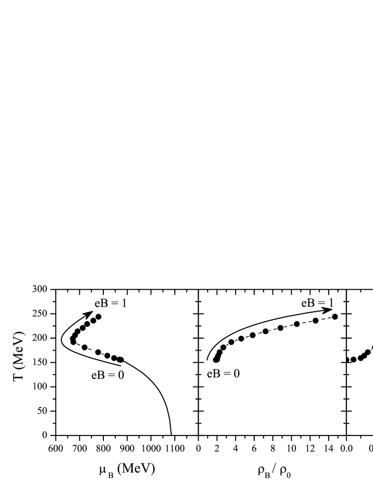
Figure 1: Location of the CEP on a diagram $T$ vs the baryonic chemical potential (left), vs the baryonic density (middle), and vs magnetic field (right) for Case IA.

In the present study we consider the PNJL model with equal quark chemical potentials, $\mu_{u}=\mu_{d}=\mu_{s}$, which corresponds to zero charge (or isospin) chemical potential and zero strangeness chemical potential ($\mu_{Q}=\mu_{S}=0$).

In Miransky:2002rp , it was shown that the running coupling decreases with the magnetic field strength. Consequently, in the NJL model the coupling $G_{s}$, which can be seen as $\propto\alpha_{s}$, must decrease with an increasing magnetic field strength. Since there is no LQCD data available for $\alpha_{s}(eB)$, by using the NJL model it is possible to fit $G_{s}(eB)$ in order to reproduce the pseudocritical chiral transition temperatures, $T_{c}^{\chi}(eB)$, obtained in LQCD calculations at $\mu_{B}=0$ baliJHEP2012 . The resulting fit function that reproduces the $T_{c}^{\chi}(eB)$ is Ferreira:2014kpa

$$G_{s}(\zeta)=G_{s}^{0}\left(\frac{1+a\,\zeta^{2}+b\,\zeta^{3}}{1+c\,\zeta^{2}+d\,\zeta^{4}}\right),$$ (7)

with $a=0.0108805$, $b=-1.0133\times 10^{-4}$, $c=0.02228$, and $d=1.84558\times 10^{-4}$, where $\zeta=eB/\Lambda_{\text{QCD}}^{2}$ and $\Lambda_{\text{QCD}}=300$ MeV.

By using $G_{s}(eB)$ given by Eq. (7) in the PNJL model both chiral and deconfinement transition temperatures decrease with increasing magnetic field strength due to the existing coupling between the Polyakov loop field and quarks within the PNJL model. Consequently, the coupling $G_{s}(eB)$ affects not only the chiral transition but also the deconfinement transition Ferreira:2014kpa .

Next, we will study the following scenarios for the effect of a static external magnetic field on the location of the CEP:

1. Case I with no IMC effects and the usual $G_{s}=G_{s}^{0}$:

   • Case IA, where we take $G_{V}=0$ (Sec. III.1);

   • Case IB, where we take $G_{V}\neq 0$, with $G_{V}=\alpha G_{s}^{0}$ (Sec. III.2).

2. Case II with IMC effects, described by $G_{s}(eB)$ given by Eq. (7):

   • Case IIA, where we take $G_{V}=0$, (Sec. IV.1);

   • Case IIB, with $G_{V}=\alpha G_{s}(eB)$, meaning that the stronger the magnetic field the weaker the vector and scalar interactions, (Sec. IV.2);

   • Case IIC, with a fixed $G_{V}=\alpha G^{0}_{s}$ (Sec. IV.2).

III The influences of an external magnetic field and of the vector interaction on the location of the CEP

The influence of the repulsive vector coupling on magnetized quark matter was investigated in Denke:2013gha by using the SU(2) version of the NJL model. Here, we will use the (2+1) PNJL model. We start our study by setting $G_{V}=0$. In a second step we consider $G_{V}\neq 0$.

III.1 $G_{V}=0$

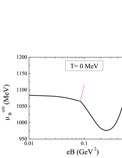
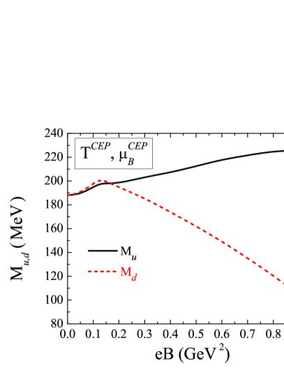
Figure 2: The critical chemical potential at $T=0$ MeV versus the magnetic field (left panel) and the $u$, $d$-quark constituent masses at the CEP as a function of the magnetic field intensity.

Figure 3: Effect of the strength of the vector interaction on the location of the CEP on a diagram $T$ vs the baryonic chemical potential (left) and $T$ vs the baryonic density (right).

The $T-\mu_{B}$ phase diagram obtained with $G_{V}=0$ (Case IA) is presented in the left panel of Fig. 1 and shows a trend very similar to that of the results previously obtained for the NJL in Avancini:2012ee : as the intensity of the magnetic field increases, the temperature at which the CEP occurs ($T^{\text{CEP}}$) increases monotonically (see Fig. 1 right panel) and the corresponding baryonic chemical potential ($\mu_{B}^{\text{CEP}}$) decreases until the critical value $eB\sim 0.4$ GeV² is reached; for stronger magnetic fields both $T^{\text{CEP}}$ and $\mu_{B}^{\text{CEP}}$ increase. In the middle panel of Fig. 1 the CEP is given in a $T$ versus baryonic density, $\rho_{B}/\rho_{0}$, plot, and it can be seen that as the magnetic field increases from 0 to 1 GeV², $\rho^{\text{CEP}}_{B}$ always increases.

To understand these behaviors at finite density we start by considering the case at $T=0$ where a first order phase transition takes place. In the left panel of Fig. 2, we present the critical chemical potential, $\mu_{B}^{\text{crit}}$, at which the first order phase transition occurs. The pattern followed by $\mu_{B}^{\text{crit}}$ at $T=0$ in the PNJL model is similar, although for smaller values, to the one reported in Avancini:2012ee at $T=1$ MeV and also at higher temperatures: slow decrease for $0<eB<0.06$ GeV², faster decrease until $0.12-0.18$ GeV², and monotonical increase afterwards. We verify a lowering of $\mu_{B}^{\text{crit}}$ with $B$ until $eB=0.25$ GeV². The slow decrease in $\mu_{B}^{\text{crit}}$ for increasing magnetic field strength in the range $0\leq eB\lesssim 0.08$ GeV² is followed by a faster decrease for $0.08\lesssim eB\lesssim 0.25$ GeV². Stronger field strengths result in a monotonically increasing $\mu_{B}^{\text{crit}}$. This change in behavior corresponds to the point where just one Landau level (LL) is filled for each flavor in the partially chiral restored phase. Indeed, the stronger the magnetic field, the larger the spacing between the levels.

At $T=\mu_{B}=0$ a stronger magnetic field results in an increase of the mass of the quarks (the increase is larger for $M_{u}$ than $M_{d}$ due to the difference in electric charges). At finite density, however, $\mu_{B}^{\text{crit}}$ starts to decrease with increasing magnetic fields, indicating an easier transition to the partially chiral restored phase Preis:2010cq . This result was already seen in Avancini:2012ee . For $eB$ above $0.25$ GeV², $\mu_{B}^{\text{crit}}$ increases.

Also noteworthy to point out is the existence of a range of magnetic fields, $0.083\lesssim eB\lesssim 0.1$ GeV², where at least two first order phase transitions occur (see Fig. 2, left panel), in accordance with what was found in the SU(2) Denke:2013gha ; Allen:2013lda and SU(3) NJL models Grunfeld:2014qfa . This cascade of transitions will result in the existence of multiple CEPs at finite temperature. The CEP on which we focus most of our attention in the present and next sections is the one that subsists to the highest temperature.

As was discussed above, in the weak magnetic field regime an increasing magnetic field results in a smaller critical chemical potential for the first order transition at $T=0$, even if the quarks’ masses have already started to increase. As this corresponds to a shift of the first order transition line toward a smaller chemical potential, the observed decrease in $\mu_{B}^{\text{CEP}}$ follows naturally. This effect is dominant over that of the increase of the quark masses at the CEP (both quark masses at the CEP increase with magnetic field strength for $eB\lesssim 0.125$ GeV²) which should hinder the first order partial chiral restoration (see Fig. 2, right panel). A similar behavior is also obtained within the NJL model used in Avancini:2012ee .

Above a critical strength for the magnetic fields, $eB\gtrsim 0.125$ GeV², there is a clear asymmetry in the CEP quark mass response to an increasing magnetic field strength: a strong decrease in $M_{d}$ as opposed to the smooth increase in $M_{u}$ (due to the charge difference the $d$-quark coupling to the magnetic field is weaker). This behavior is accompanied by an increase of the baryonic density at which the CEP occurs (Fig. 1, right panel).

For stronger magnetic fields ($eB\gtrsim 0.4$ GeV²) both $T^{\text{CEP}}$ and $\mu_{B}^{\text{CEP}}$ increase. This can be understood as a result of a decreasing number of occupied LL due to the large intensity of the field and the greater difficulty in restoring chiral symmetry.

III.2 $G_{V}\neq 0$

The role of the vector interaction in the PNJL was studied in detail in Fukushima:2008wg ; Friesen:2014mha . The main conclusion was that the CEP can be absent when the value of the coupling $G_{V}$ is greater than a critical value $G_{V}^{\text{crit}}$. With the present parametrization this critical value is when $\alpha\approx 0.71$, i.e, $G_{V}^{\text{crit}}\approx 0.71G_{s}^{0}$ (see both panels of Fig. 3). As the value of the coupling $G_{V}$ is increased from 0 to $G_{V}^{\text{crit}}$ the first order phase transition is weakened and the CEP occurs at lower temperatures and larger chemical potentials but smaller densities.

When the external magnetic field and the vector interaction are taken into account simultaneously, the scenario becomes more complex. In our discussion we will fix $\alpha=0.25$ ($G_{V}=0.25G_{s}^{0}$) and $eB=0.09$ GeV² to compare to cases with $G_{V}=0$ and $G_{V}=0.25G_{s}^{0}$ at zero magnetic field. The results are presented in Fig. 4, left panel. In the following we will show that for the light sector the (2+1) PNJL model is in agreement with the SU(2) NJL model (see Denke:2013gha for details).

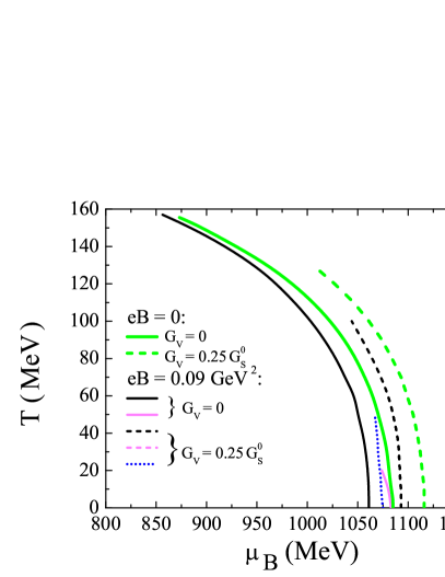
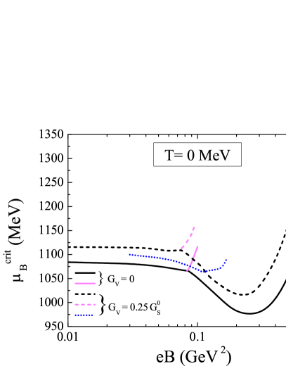
Figure 4: QCD phase diagram in a $T-\mu_{B}$ plot for Cases IA and IB, not including IMC effects, discussed in the text, left panel. The critical chemical potential as a function of the magnetic field intensity at $T=0$, right panel. The green thick lines correspond to no magnetic field, and dashed (full) lines were obtained with (without) the vector interaction.

We start by exploring in detail the phase diagram in the presence of a magnetic field $eB=0.09$ GeV² at $G_{V}=0$ where two first order phase transitions in cascade occur at $T=0$. We identify a decrease of $\mu_{B}^{\text{crit}}$ for both transitions (see black and red full lines of Fig. 4 left panel) when compared with the transition at zero magnetic field (green full line in the same figure).

At $T=0$ these transitions occur for a given $\mu_{B}$ at which the gap equations have two stable solutions ($M_{i}^{I}$ and $M_{i}^{II}$) leading to the coexistence of two different quark masses at the same pressure and temperature. The first transition occurs at $\mu_{B}=1061$ MeV, being $M_{u(d)}^{I-1\text{st}}=378.7\,(374.8)$ MeV and $M_{u(d)}^{II-1\text{st}}=166.0\,(158.9)$ MeV, and the second transition occurs at $\mu_{B}=1083$ MeV, where $M_{u(d)}^{I-2\text{nd}}=149.8\,(141.4)$ MeV and $M_{u(d)}^{II-2\text{nd}}=49.4\,(49.0)$ MeV.

At this point some other relevant aspects of these results are worth highlighting:

1. At $\mu_{B}=0$ and $eB=0.09$ GeV² we have the magnetic catalysis effect as $M_{u}$ and $M_{d}$ are higher than the respective vacuum values ($M_{u}^{\text{vac}}=M_{d}^{\text{vac}}=367.7$ MeV);

2. At the first phase transition the values of $M_{u(d)}^{II-1\text{st}}=166.0\,(158.9)$ MeV are still far from the respective current values ($m_{u}=m_{d}=5.5$ MeV), and a second transition is needed to bring $M_{u(d)}^{II-2\text{nd}}$ to values closer to $m_{u(d)}$ which is consistent with a region where the chiral symmetry is partially restored.

3. At the second phase transition $M_{u(d)}^{II-2\text{nd}}=49.4\,(49.0)$ MeV and these values are already smaller than $M_{u}^{II}=M_{d}^{II}=52.2$ MeV at $eB=0$.

4. If we take the chiral limit for the light sector, $m_{u}=m_{d}=0$, the restoration of chiral symmetry, $M_{u}=M_{d}=0$, does not coincide with the first phase transition: at $\mu_{B}=1012$ MeV there is a jump in the quarks’ masses from $M_{u(d)}^{I-1\text{st}}=366.5\,(362.5)$ MeV to $M_{u(d)}^{II-1\text{st}}=36.1\,(33.5)$ MeV but only at $\mu_{B}=1017$ MeV we have $M_{u}=M_{d}=0$. This is a direct manifestation of the condensate enhancement by magnetic catalysis.

5. At finite temperature the second transition exists only at low temperatures and turns into a CEP at around $T\sim 20$ MeV (see red full line, left panel of Fig. 4). Increasing the temperature, the remaining first order transition will subsist until $T^{\text{CEP}}=157$ MeV and $\mu_{B}^{\text{CEP}}=856$ MeV, closer to the CEP for $eB=0$ ($T^{\text{CEP}}=156$ MeV, $\mu_{B}^{\text{CEP}}=873$ MeV Costa:2013zca ).

When the vector interaction is also taken into account in the presence of a magnetic field, two competing effects come into play: on the one hand, an increase of $G_{V}$ at $eB=0$ weakens the first order phase transition which leads to the disappearance of the CEP in the $\mu_{B}$ axis (this can be seen in the left panel of Fig. 4 where the green dashed line shows how $G_{V}$ affects the first order phase transition); on the other hand, an increase of the magnetic field at $G_{V}=0$ has an opposite influence in the first order transition and CEP location, moving the transition line to smaller chemical potentials, at least until $eB=0.4$ GeV², as shown by the black line ($eB=0.09$ GeV²) in the left panel of Fig. 4. Besides, as we already saw, the presence of a strong enough magnetic field can drive multiple CEPs due to the existence of several first order transitions at $T=0$.

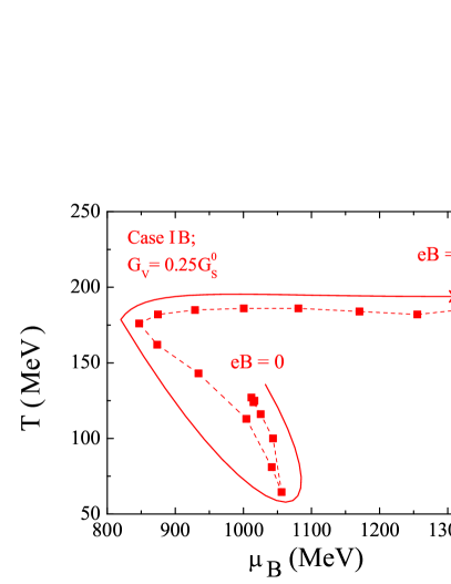
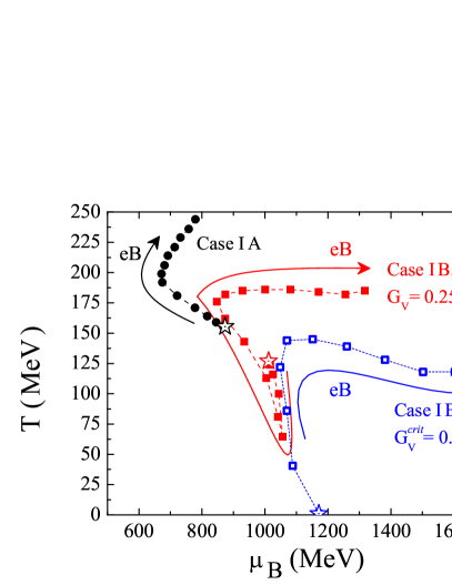
Figure 5: The location of the CEP for Case IB, with the inclusion of the vector interaction and no IMC, the results for Case IB with $\alpha=0.25$ and 0.71 are compared with Case IA, with no vector interaction. The thin arrows indicate the direction of increasing magnetic field intensity.

Now, we discuss the case $G_{V}=0.25G_{s}^{0}$ starting with $T=0$ in the presence of an external magnetic field. As $B$ increases, several first order transitions in cascade take place, similar to the $G_{V}=0$ results. The critical chemical potential at which the transitions occur is shown in the right panel of Fig. 4 (dashed lines): there is a range of magnetic fields, $0.03\lesssim eB\lesssim 0.11$ GeV², where two transitions occur and a range, $0.07\lesssim eB\lesssim 0.09$ GeV², where three transitions in cascade coexist. A first conclusion about the combined effect of $B$ and $G_{V}$ is the appearance of intermediate transitions for a wider range of magnetic fields.

Let us fix once again $eB=0.09$ GeV², a scenario where we have three phase transitions: compared with the $eB=0$ result (green dashed line), two transitions occur at lower $\mu_{B}$ (black and blue dashed lines in Fig. 4, left panel) and a third one at higher $\mu_{B}$ (red dashed line in the same panel). At finite temperatures the phase transitions will give rise to three CEPs. The CEP with the larger temperature, $T^{\text{CEP}}=100$ MeV and $\mu_{B}^{\text{CEP}}=1044$ MeV, (black dashed line in Fig. 4, left panel), has a lower temperature and larger chemical potential than the CEP at $eB=0$.

In Fig. 5 left panel, the location of the CEP obtained with $G_{V}=0.25\,G_{s}$ is plotted for different values of the magnetic field, the thin arrowed line shows the direction of increasing fields. Going along the direction of increasing fields, there is a first region corresponding to the weaker magnetic fields $B<0.1$ GeV², where the CEP temperature decreases and CEP chemical potential increases. Next, for $0.1<eB\lesssim 0.4$ GeV² the CEP temperature increases and the CEP chemical potential decreases, and finally for stronger fields the CEP chemical potential increases while the CEP temperature remains practically unchanged.

For $B<0.1$ GeV², $\mu_{B}^{\text{CEP}}$ increases slightly and the respective baryonic density decreases, the magnetic field having an effect that adds to the one of $G_{V}$. In this region $G_{V}$ is dominant and weakens the first order phase transition. This effect was clarified in Denke:2013gha : although the effect of $G_{V}$ goes always in the direction of reducing the density at the first order phase transition, the magnetic field does not present a monotonic behavior as seen for the scenario without the vector term.

Above $B=0.1$ GeV², the effect of $B$ on the CEP location is close to the one obtained for $G_{V}=0$, except that for $eB\gtrsim 0.4$ GeV² the CEP temperature keeps increasing if $G_{V}=0$, while for a finite $G_{V}$ this trend is strongly reduced and the temperature does not change much; compare black and red curves of Fig. 5 right panel.

III.3 $G_{V}=G_{V}^{\text{crit}}$

Finally, we investigate the case $G_{V}^{\text{crit}}\approx 0.71G_{s}^{0}$. The results are presented in the right panel of Fig. 5 (blue curves). The effect of the field is to restore a first order phase transition.

For $0.01\lesssim eB\lesssim 0.1$ GeV² a very complex structure of multiple first order transitions appears at $T=0$. These multiple transitions will be washed out with the increasing of the temperature until just one CEP remains. However, more than one CEP can occur at very close temperatures like the scenario found in Costa:2013zca . Above 0.1 GeV² this complex structure disappears (in the right panel of Fig. 5 we start to represent CEP for $eB>0.1$ GeV²). For $0.1\lesssim eB\lesssim 0.4$ GeV² we verify that the larger $eB$ the larger $T^{\text{CEP}}$ until a maximum $T\sim 145$ MeV is reached. In the same range, the CEP chemical potential decreases slightly for $eB<0.3$ GeV², and increases for stronger fields.

Increasing further the magnetic field, i.e. $eB>0.4$ GeV², the $\mu_{B}^{\text{CEP}}$ increases while the temperature does not change much until $eB=1$ GeV², showing also stabilization of the CEP temperature even if weaker than the one obtained for $G_{V}=0.25\,G_{s}$. The number of occupied LL becomes quite small. Indeed, taking $eB=0.4$ GeV², the number of occupied LL at the CEP decreases with increasing $G_{V}$. The behavior obtained is the result of a clear competition between the magnetic field that disfavors chiral symmetry restoration and the vector interaction with an opposite effect.

IV The influence of the inverse magnetic catalysis in the location of the critical end point

In this section we will investigate the influence, in the location of the CEP, of the IMC effect observed in LQCD calculations at zero chemical potential. First, the discussion will not include the vector interaction, Case IIA (Sec. IV.1) and next the IMC effects will be considered together with the vector interaction, Cases IIB and IIC (Sec. IV.2).

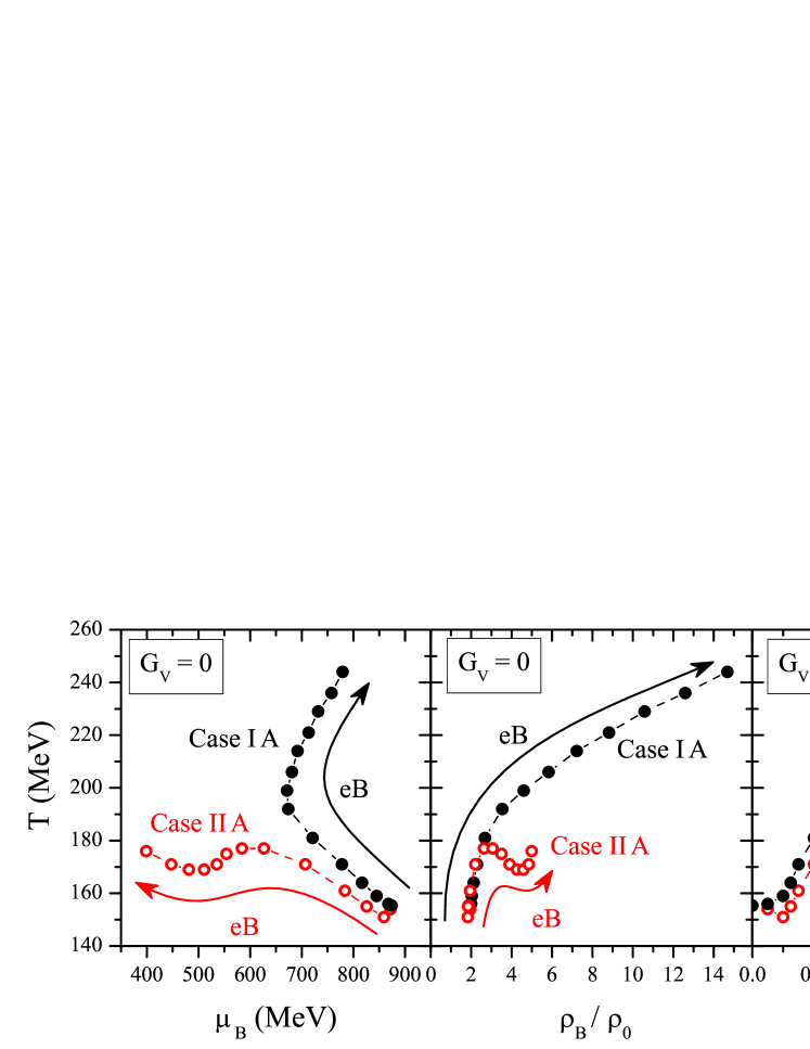
Figure 6: Location of the CEP, $T^{\text{CEP}}$ versus $\mu_{B}^{\text{CEP}}$ (left panel) and $T^{\text{CEP}}$ versus $\rho_{B}^{\text{CEP}}$ (right panel), for different intensities of the magnetic field and excluding the vector interaction, without IMC effects $G_{s}=G_{s}^{0}$ (red curve) and with IMC effects $G_{s}=G_{s}(eB)$ (black curve).

IV.1 $G_{V}=0$

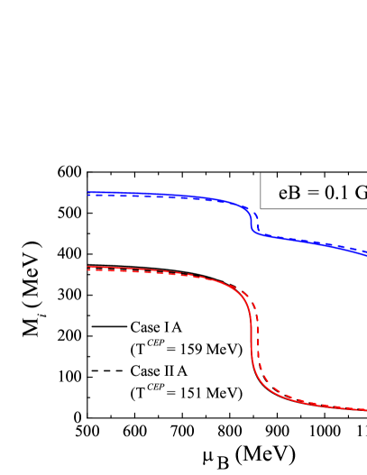
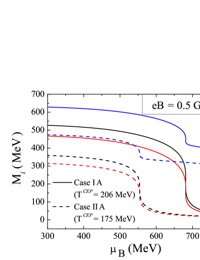
Figure 7: Masses of the quarks as a function of $\mu_{B}$ for two intensities of the magnetic field: $eB=0.1$ GeV² (left) and : $eB=0.5$ GeV² (right), at the respective $T^{\text{CEP}}$.

The effect of the IMC on the CEP location excluding the vector interaction, Case IIA, is presented in Fig. 6 (red points) in the $T-\mu_{B}$ plane (left panel) and in the $T-\rho_{B}/\rho_{0}$ plane (middle panel), for different intensities of the magnetic field, and in the $T-eB$ plane (right panel). For comparison we include in the same figure the CEP location without IMC effects, Case IA (black curve). We clearly observe a different behavior between these two scenarios: at $B=0$ both CEPs coincide but, already for small values of $B$, the IIA CEP is moved to lower temperatures and chemical potentials, keeping, however, a similar behavior to IA until $eB\sim 0.3$ GeV². The large differences start for stronger magnetic fields: in Case IIA the position of the CEP oscillates between $T\approx 169$ and $T\approx 177$ MeV while the chemical potential takes increasingly smaller values; in Case IA both values of $T$ and $\mu_{B}$ for the CEP increase (see black curve, left panel of Fig. 6). In the middle panel of Fig. 6 the position of the CEP in the $T-\rho_{B}/\rho_{0}$ plane is presented. Comparing Cases IA and IIA, it is found that the IMC effect on the CEP results on its shift to smaller temperatures and densities especially for higher values of the magnetic field.

The reason for these behaviors lies in the fact that the weakening of the coupling $G_{s}(eB)$ will make the restoration of chiral symmetry easier. Increasing the magnetic field is not sufficient to counteract this effect, as can be seen in Fig. 7 where we plot the quark masses ($M_{u}$: black line; $M_{d}$: red line; $M_{s}$: blue line) as a function of $\mu_{B}$ for the respective $T^{\text{CEP}}$ at $eB=0.1$ and $eB=0.5$ GeV². At $eB=0.1$ GeV², left panel, $G_{s}$ is barely affected by the magnetic field when IMC effects are included and the values of the quark masses are very close to each other for both cases: in Case IIA the CEP occurs at smaller temperatures and at near, slightly higher, chemical potentials. When $eB=0.5$ GeV², right panel, the quark masses in Case IA have increased with respect to the $eB=0$ case (due to the MC effect), making the restoration of chiral symmetry more difficult to achieve. However, when $G_{s}=G_{s}(eB)$, Case IIA, the masses of the quarks are smaller than their $eB=0$ value (due to IMC effect), leading to a faster restoration of chiral symmetry at small temperatures and chemical potentials.

Eventually, with the increase of $eB$ the CEP would move toward $\mu_{B}=0$, and the deconfinement and chiral phase transitions would always be of first order.

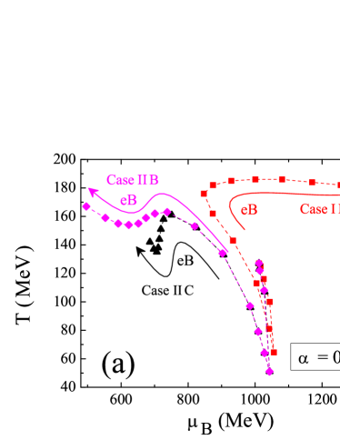
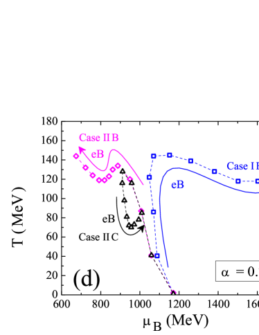
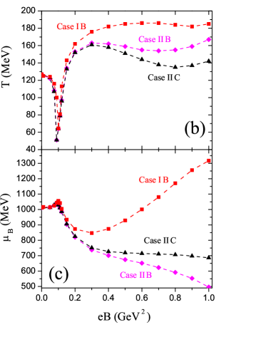
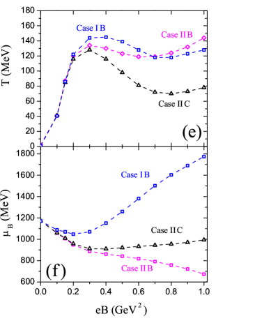
Figure 8: The location of the CEP: (a) and (d) $T$ versus $\mu_{B}$, for different intensities of the magnetic field; (b) and (e) $T$ as a function of $eB$; (c) and (f) $\mu_{B}$ versus $eB$, for the vector interaction $\alpha=0.25$ [left, (a), (b) and (c) panels] and $\alpha=0.71$ [right, (d), (e) and (f) panels]. The red and blue curves were obtained with no IMC effects and correspond to Cases IA and IB. The IMC effects and vector interaction were included in the black curves ($G_{V}$ is fixed) and magenta ($G_{V}$ weakens with an increasing $eB$). For more details see the text at the end of Sec. IV.

IV.2 $G_{V}\neq 0$

In this subsection we discuss the role of the vector interaction in the location of the CEP of magnetized quark matter taking into account explicitly the inverse magnetic catalysis at finite $T$ through the renormalization of the coupling $G_{s}$ due to the presence of the magnetic field. We will consider two scenarios, with or without an explicit dependence of $G_{V}$ on the magnetic field: $G_{V}=\alpha G_{s}(eB)$ (Case IIB), and $G_{V}=\alpha G^{0}_{s}$ (Case IIC). For the constant $\alpha$ we will take a general value $\alpha=0.25$ (left panels of Fig. 8), and the critical value discussed above, $\alpha=0.71$ (right panels of Fig. 8) .

We will first consider $\alpha=0.25$ [see panels (a), (b) and (c) of Fig. 8]. In these panels, the red curves correspond to Case IB with $G_{V}=0.25G_{s}^{0}$, already presented in Fig. 5, and the black and the blue curves are for $G_{s}=G_{s}(eB)$ and, respectively, for $G_{V}=0.25G_{s}(eB)$ (Case IIB) and $G_{V}=0.25G_{s}^{0}$ (Case IIC). When the IMC effects are included in the definition of the scalar coupling, and the vector term is taken into account, it is seen that for small values of $B$ the CEP moves to lower values of $T$ and slightly higher values of $\mu_{B}$ (although a bit lower than in Case IIA), in both Cases IIB and IIC [see panels 8(b) and 8(c), respectively]. Although the coupling $G_{s}(eB)$, and consequently also $G_{V}$ in Case IIB, is slightly affected by the magnetic field, the overall balance between the contributions of the attractive and the repulsive interactions is almost unchanged.

For $0.09<eB\lesssim 0.3$GeV² the behavior for all three cases with $G_{V}\neq 0$, IB, IIB, and IIC, is very similar to the one found with $G_{V}=0$ (Cases IA and IIA): the critical temperature increases [see panel 8(b)] and the critical chemical potential decreases [see panel 8(c)].

However, differences occur for stronger magnetic fields. When $eB\gtrsim 0.3$GeV², the CEP moves to smaller chemical potentials while the temperature does not change much in Case IIB. On the other hand, in Case IIC, with a coupling $G_{V}$ that does not change with $B$, the vector contribution becomes more important than the catalysis effect of the magnetic field, since this last effect has been weakened by a weak coupling $G_{s}(eB)$. Consequently, as soon as $G_{s}$ is sufficiently weak, the effect of $G_{V}$ is seen in the decrease of $T^{\text{CEP}}$ [see panel 8(b)], while $\mu_{B}^{\text{CEP}}$ practically does not change [see panel 8(c)].

When $\alpha=0.71$ [see panels (d), (e) and (f) of Fig. 8] the CEP, for all cases with $G_{V}\neq 0$, shows a similar behavior as the field is increased from $eB=0$, when $T^{\text{CEP}}=0$ MeV and $eB\sim 0.3$ GeV²: the CEP moves to lower chemical potentials [see panel 8(f)] and the critical temperature to larger values [see panel 8(e)]. When the IMC effect is included, Cases IIB and IIC, the curves overlap due to a weakened coupling $G_{s}(eB)$. Above $eB\sim 0.3$ GeV², in Case IIB the CEP occurs for smaller values of $\mu_{B}^{\text{CEP}}$ while $T^{\text{CEP}}$ does not change much, a behavior also occurring for $\alpha=0.25$. In Case IIC, with $G_{V}=0.71G_{s}^{0}$, the trend is different from the corresponding one obtained with $\alpha=0.25$: the coupling $G_{s}$ becomes sufficiently weak with respect to the magnitude of $G_{V}$ and the effect of the vector coupling is seen in the decrease of $T^{\text{CEP}}$ and the weak increase of $\mu_{B}^{\text{CEP}}$. For $eB>0.8$ GeV² the effect of the magnetic field clearly overlaps the effect of $G_{V}$, and the CEP goes to higher temperatures and chemical potentials as in Case IB without the IMC effect ($G_{V}=0.71G_{s}^{0}$).

It is also interesting to study the effect of the magnetic field on the CEP baryonic density. In Fig. 9 the CEP location is plotted as a function of this quantity for different scenarios discussed in the present and previous sections. It is seen that the CEP baryonic density is not much affected by the field, the only exception if the different behavior of Case IB for the stronger fields, the CEP temperature being the property that distinguishes the different scenarios.

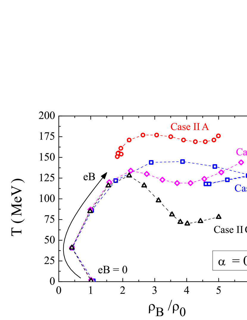
Figure 9: The CEP location on the T-$\rho_{B}$ plane. Cases IIA, IIB and IIC with IMC effects are compared with Case IB without IMC effects. Case IIA is the only scenario excluding the vector interaction.

V Conclusions

In the present work we have discussed the possible consequences of the IMC effect on the location of the CEP. The discussion has been performed within the (2+1) PNJL model with the possible inclusion of the vector interaction. Within this model the IMC effect is described by considering a scalar coupling that weakens with the increase of the magnetic field as proposed in Ferreira:2014kpa . The dependence of the coupling on the magnetic field has been fitted to the LQCD calculations of the transition temperature at zero chemical potential, which show a decreasing crossover temperature with an increase of the magnetic field for intensities below $eB=1$ GeV².

The main conclusion of the present work is that the IMC effect will have noticeable effects on the location of the CEP. If the vector interaction is switched off, the CEP will occur at increasingly smaller chemical potentials and at a practically unchanged temperature if the field satisfies $eB\gtrsim 0.3$ GeV². This behavior is contrary to the findings of Avancini:2012ee with SU(3) NJL with constant couplings, where it was shown that above $0.3$ GeV², both $T^{\text{CEP}}$ and $\mu_{B}^{\text{CEP}}$ increase. Also the baryonic density at the CEP is affected: including IMC effects it increases only $~{}1/3$ of the expected if IMC effects were not considered, making the CEP much more accessible in the laboratory. However, for weaker fields, $eB<0.3$ GeV², both scenarios give similar results.

If the vector interaction is included, we must consider two scenarios: a strong enough vector interaction will turn the first order deconfinement/chiral transition into a crossover Fukushima:2008wg or, on the contrary, the vector interaction is not strong enough to wash out the CEP, but moves its location to smaller temperatures and baryonic densities and to larger chemical potentials. For the first scenario we have confirmed within the (2+1) PNJL model the findings of Denke:2013gha obtained with the SU(2) NJL model, showing that a strong magnetic field would transform the crossover into a first order phase transition. With respect to the second scenario, we have shown that for sufficiently small fields, the repulsive effect of the interaction is stronger than the MC effect originated by the magnetic field, and the CEP location occurs at smaller temperatures and slightly larger chemical potentials. The decrease of the CEP temperature could be quite large, for $\alpha=0.25$: $T^{\text{CEP}}$ suffers a reduction above 60 MeV when $eB$ goes from 0 to 0.09 GeV². Both effects corresponding to the two scenarios move the CEP to regions of temperature and density in the phase diagram that could be more easily accessible to HIC.

For larger fields, 0.09 GeV${}^{2}<eB\lesssim 0.3$ GeV² the magnetic field wins and $\mu_{B}^{\text{CEP}}$ decreases while $T^{\text{CEP}}$ increases, showing a behavior similar to the corresponding one in the absence of a vector interaction. Above $eB\gtrsim 0.3$ GeV² the CEP chemical potential increases but the CEP temperature keeps practically unchanged.

The joint effect of the vector interaction and the IMC effect of the magnetic field depends strongly on the magnitude of the magnetic field and whether the vector coupling becomes weaker with the magnetic field. We have considered two scenarios: a constant $G_{V}$ and a $G_{V}$ that weakens when the magnetic field intensity increases. In the second case the location of the CEP for very strong magnetic fields is not much affected by the vector contribution, the magnetic field defining the structure of the phase transition. If, however, the vector coupling is not affected by the magnetic field, the weakening of the scalar coupling with the increase of the magnetic field intensity leads to the dominance of the vector contribution, which translates into a reduction of the CEP temperature. An overall general conclusion is the reduction of the CEP temperature when the vector interaction is included. This effect will be quite strong if the vector coupling does not become weaker when the magnetic field intensity increases.

Acknowledgments: This work was supported by “Fundação para a Ciência e Tecnologia”, Portugal, under the Grants No. SFRH/BPD/102273/2014 (P. C.), No. SFRH/BD/51717/2011 (M. F.), and No. SFRH/BPD/63070/2009 (J. M.). This work was partly supported by Project PEst-OE/FIS/UI0405/2014 developed under the initiative QREN financed by the UE/FEDER through the program COMPETE-“Programa Operacional Factores de Competitividade”, by ”Conselho Nacional de Desenvolvimento Científico e Tecnológico” (CNPq), Brazil, and by “NewCompstar”, COST Action MP1304.

References

- (1) Z. Fodor and S. D. Katz, J. High Energy Phys. 0404, 050 (2004) [hep-lat/0402006].
- (2) P. de Forcrand and O. Philipsen, Nucl. Phys. B673, 170 (2003) [hep-lat/0307020].
- (3) C. S. Fischer, J. Luecker, and C. A. Welzbacher, Phys. Rev. D 90, no. 3, 034022 (2014) [arXiv:1405.4762 [hep-ph]].
- (4) P. Costa, M. C. Ruivo, and C. A. de Sousa, Phys. Rev. D 77, 096001 (2008) [arXiv:0801.3417 [hep-ph]]; P. Costa, C. A. de Sousa, M. C. Ruivo, and Y. L. Kalinovsky, Phys. Lett. B 647, 431 (2007) [hep-ph/0701135].
- (5) J. Moreira, J. Morais, B. Hiller, A. A. Osipov, and A. H. Blin, Phys. Rev. D 91, 116003 (2015) [arXiv:1409.0336 [hep-ph]].
- (6) P. Costa, C. A. de Sousa, M. C. Ruivo, and H. Hansen, Europhys. Lett. 86, 31001 (2009) [arXiv:0801.3616 [hep-ph]]; P. Costa, M. C. Ruivo, C. A. de Sousa, and H. Hansen, Symmetry 2, 1338 (2010) [arXiv:1007.1380 [hep-ph]].
- (7) B. I. Abelev et al. [STAR Collaboration], Phys. Rev. C 81, 024911 (2010) [arXiv:0909.4131 [nucl-ex]]
- (8) L. Adamczyk et al. [STAR Collaboration], Phys. Rev. Lett. 113, 092301 (2014) [arXiv:1402.1558 [nucl-ex]].
- (9) L. Adamczyk et al. [STAR Collaboration], Phys. Rev. Lett. 112, no. 3, 032302 (2014) [arXiv:1309.5681 [nucl-ex]].
- (10) Y. Akiba et al., arXiv:1502.02730 [nucl-ex].
- (11) M. Gazdzicki [NA49 and NA61/SHINE Collaborations], J. Phys. G 38, 124024 (2011) [arXiv:1107.2345 [nucl-ex]].
- (12) P. Costa, M. Ferreira, H. Hansen, D. P. Menezes, and C. Providência, Phys. Rev. D 89, no. 5, 056013 (2014) [arXiv:1307.7894 [hep-ph]].
- (13) S. S. Avancini, D. P. Menezes, M. B. Pinto, and C. Providencia, Phys. Rev. D 85, 091901 (2012) [arXiv:1202.5641 [hep-ph]].
- (14) M. Ruggieri, L. Oliva, P. Castorina, R. Gatto, and V. Greco, Phys. Lett. B 734, 255 (2014) [arXiv:1402.0737 [hep-ph]].
- (15) V. Skokov, A. Y. Illarionov, and V. Toneev, Int. J. Mod. Phys. A 24, 5925 (2009); V. Voronyuk, V. Toneev, W. Cassing, E. Bratkovskaya, V. Konchakovski, and S. Voloshin, Phys. Rev. C 83, 054911 (2011); D. E. Kharzeev, L. D. McLerran, and H. J. Warringa, Nucl. Phys. A 803, 227 (2008).
- (16) F. Bruckmann, G. Endrödi, and T. G. Kovacs, J. High Energy Phys. 1304, 112 (2013) [arXiv:1303.3972 [hep-lat]].
- (17) G. S. Bali, F. Bruckmann, G. Endrödi, Z. Fodor, S. D. Katz, S. Krieg, A. Schäfer, and K. K. Szabó, J. High Energy Phys. 1202, 044 (2012) [arXiv:1111.4956 [hep-lat]].
- (18) G. S. Bali, F. Bruckmann, G. Endrödi, Z. Fodor, S. D. Katz, and A. Schäfer, Phys. Rev. D 86, 071502 (2012) [arXiv:1206.4205 [hep-lat]].
- (19) E. -M. Ilgenfritz, M. Muller-Preussker, B. Petersson, and A. Schreiber, Phys. Rev. D 89, 054512 (2014) arXiv:1310.7876 [hep-lat].
- (20) M. D’Elia, S. Mukherjee, and F. Sanfilippo, Phys. Rev. D 82, 051501 (2010) [arXiv:1005.5365 [hep-lat]].
- (21) V. G. Bornyakov, P. V. Buividovich, N. Cundy, O. A. Kochetkov, and A. Schäfer, arXiv:1312.5628 [hep-lat].
- (22) J. O. Andersen, W. R. Naylor, and A. Tranberg, arXiv:1311.2093 [hep-ph].
- (23) W. j. Fu, Phys. Rev. D 88, no. 1, 014009 (2013) [arXiv:1306.5804 [hep-ph]].
- (24) M. Ferreira, P. Costa, D.P. Menezes, C. Providência, and N.N. Scoccola, Phys. Rev. D 89, 016002 (2014). [arXiv:1305.4751 [hep-ph]].
- (25) M. Ferreira, P. Costa, and C. Providência, Phys. Rev. D 89, no. 3, 036006 (2014) [arXiv:1312.6733 [hep-ph]].
- (26) M. Ferreira, P. Costa, and C. Providência, Phys. Rev. D 90, no. 1, 016012 (2014) [arXiv:1406.3608 [hep-ph]].
- (27) V. A. Miransky and I. A. Shovkovy, Phys. Rev. D 66, 045006 (2002) [hep-ph/0205348].
- (28) R. L. S. Farias, K. P. Gomes, G. I. Krein, and M. B. Pinto, Phys. Rev. C 90, no. 2, 025203 (2014) [arXiv:1404.3931 [hep-ph]].
- (29) M. Ferreira, P. Costa, O. Lourenço, T. Frederico, and C. Providência, Phys. Rev. D 89, no. 11, 116011 (2014) [arXiv:1404.5577 [hep-ph]].
- (30) J. Chao, P. Chu, and M. Huang, Phys. Rev. D 88, 054009 (2013) [arXiv:1305.1100 [hep-ph]].
- (31) K. Fukushima and Y. Hidaka, Phys. Rev. Lett. 110, no. 3, 031601 (2013) [arXiv:1209.1319 [hep-ph]].
- (32) A. Ayala, M. Loewe, A. J. Mizher, and R. Zamora, Phys. Rev. D 90, no. 3, 036001 (2014) [arXiv:1406.3885 [hep-ph]]; A. Ayala, J. J. Cobos-Martínez, M. Loewe, M. E. Tejeda-Yeomans, and R. Zamora, Phys. Rev. D 91, no. 1, 016007 (2015) [arXiv:1410.6388 [hep-ph]].
- (33) J. Braun, W. A. Mian, and S. Rechenberger, arXiv:1412.6025 [hep-ph].
- (34) N. Mueller and J. M. Pawlowski, arXiv:1502.08011 [hep-ph].
- (35) F. Preis, A. Rebhan, and A. Schmitt, J. High Energy Phys. 1103, 033 (2011) [arXiv:1012.4785 [hep-th]].
- (36) F. Preis, A. Rebhan, and A. Schmitt, Lect. Notes Phys. 871, 51 (2013) [arXiv:1208.0536 [hep-ph]].
- (37) R. Z. Denke and M. B. Pinto, Phys. Rev. D 88, no. 5, 056008 (2013) [arXiv:1306.6246 [hep-ph]].
- (38) A. F. Garcia and M. B. Pinto, Phys. Rev. C 88, no. 2, 025207 (2013) [arXiv:1306.3090 [hep-ph]].
- (39) K. Fukushima, Phys. Rev. D 77, 114028 (2008) [Phys. Rev. D 78, 039902 (2008)] [arXiv:0803.3318 [hep-ph]].
- (40) M. Dutra, O. Lourenço, A. Delfino, T. Frederico, and M. Malheiro, Phys. Rev. D 88, no. 11, 114013 (2013) [arXiv:1312.1130 [hep-ph]].
- (41) T. Hatsuda and T. Kunihiro, Phys. Rep. 247, 221 (1994) [hep-ph/9401310].
- (42) V. Bernard, A. H. Blin, B. Hiller, U. G. Meissner, and M. C. Ruivo, Phys. Lett. B 305, 163 (1993) [hep-ph/9302245].
- (43) Luca Bonanno and Armen Sedrakian, Astron. & Astrophys. 539, A16 (2012).
- (44) D. P. Menezes, M. B. Pinto, L. B. Castro, P. Costa, and C. Providência, Phys. Rev. C 89, no. 5, 055207 (2014) [arXiv:1403.2502 [nucl-th]].
- (45) P. C. Chu, X. Wang, L. W. Chen, and M. Huang, Phys. Rev. D 91, no. 2, 023003 (2015) [arXiv:1409.6154 [nucl-th]].
- (46) K. Fukushima, Phys. Lett. B 591, 277 (2004) [hep-ph/0310121]; C. Ratti, M. A. Thaler, and W. Weise, Phys. Rev. D 73, 014019 (2006) [hep-ph/0506234].
- (47) S. P. Klevansky, Rev. Mod. Phys. 64, 649 (1992).
- (48) I. N. Mishustin, L. M. Satarov, H. Stoecker, and W. Greiner, Phys. Rev. C 62, 034901 (2000) [hep-ph/0002148].
- (49) S. Roessner, C. Ratti, and W. Weise, Phys. Rev. D 75, 034007 (2007) [hep-ph/0609281].
- (50) P. Rehberg, S. P. Klevansky, and J. Hufner, Phys. Rev. C 53, 410 (1996) [hep-ph/9506436].
- (51) D. P. Menezes, M. B. Pinto, S. S. Avancini, A. Perez Martinez, and C. Providência, Phys. Rev. C 79, 035807 (2009) [arXiv:0811.3361 [nucl-th]]; D. P. Menezes, M. B. Pinto, S. S. Avancini, and C. Providência, Phys. Rev. C 80, 065805 (2009) [arXiv:0907.2607 [nucl-th]].
- (52) P. G. Allen and N. N. Scoccola, Phys. Rev. D 88, 094005 (2013) [arXiv:1309.2258 [hep-ph]].
- (53) A. G. Grunfeld, D. P. Menezes, M. B. Pinto, and N. N. Scoccola, Phys. Rev. D 90, no. 4, 044024 (2014) [arXiv:1402.4731 [hep-ph]].
- (54) A. V. Friesen, Y. L. Kalinovsky, and V. D. Toneev, Int. J. Mod. Phys. A 30, no. 16, 1550089 (2015) [arXiv:1412.6872 [hep-ph]].