Clustering of the AKARI NEP Deep Field 24 $\mu$m selected galaxies

Abstract

Aims. We present a method of selection of 24 $\mu$m galaxies from the AKARI North Ecliptic Pole (NEP) Deep Field down to $150\mbox{ }\mu$Jy and measurements of their two-point correlation function. We aim to associate various 24 $\mu$m selected galaxy populations with present day galaxies and to investigate the impact of their environment on the direction of their subsequent evolution.

Methods. We discuss using of Support Vector Machines (SVM) algorithm applied to infrared photometric data to perform star-galaxy separation, in which we achieve an accuracy higher than 80%. The photometric redshift information, obtained through the CIGALE code, is used to explore the redshift dependence of the correlation function parameter ($r_{0}$) as well as the linear bias evolution. This parameter relates galaxy distribution to the one of the underlying dark matter. We connect the investigated sources to their potential local descendants through a simplified model of the clustering evolution without interactions.

Results. We observe two different populations of star-forming galaxies, at $z_{med}\sim 0.25$, $z_{med}\sim 0.9$. Measurements of total infrared luminosities ($L_{TIR}$) show that the sample at $z_{med}\sim 0.25$ is composed mostly of local star-forming galaxies, while the sample at $z_{med}\sim 0.9$ is composed of luminous infrared galaxies (LIRGs) with $L_{TIR}\sim 10^{11.62}L_{\odot}$. We find that dark halo mass is not necessarily correlated with the $L_{TIR}$: for subsamples with $L_{TIR}=10^{11.15}L_{\odot}$ at $z_{med}\sim 0.7$ we observe a higher clustering length ($r_{0}=6.21\pm 0.78$ $[h^{-1}\mbox{Mpc}]$) than for a subsample with mean $L_{TIR}=10^{11.84}L_{\odot}$ at $z_{med}\sim 1.1$ ($r_{0}=5.86\pm 0.69$ $h^{-1}\mbox{Mpc}$). We find that galaxies at $z_{med}\sim 0.9$ can be ancestors of present day $L_{*}$ early type galaxies, which exhibit a very high $r_{0}\sim 8$ $h^{-1}\mbox{Mpc}$.

1 Introduction

The connection between the properties of galaxies, such as morphology, luminosity, colour, surface brightness, or specific star formation rate (SFR), and the local environment in which they reside is well documented (e.g., Marinoni et al. 1999; Marinoni et al. 2002; Hogg et al. 2004; Weinmann et al. 2006; Hirschmann et al. 2013; Boselli et al. 2014; Guglielmo et al. 2015) over a wide range of redshifts. Different environments, from rich clusters to very low density areas, can have a significant influence on formation and a subsequent evolution of galaxies. A range of environmental mechanisms, such as galaxy mergers (Toomre & Toomre 1972), harrassment (Moore et al. 1996), and gas stripping (Gunn & Gott 1972) are expected to influence the determination of different galaxy properties. However, intrinsic physical processes, such as supernovae feedback (e.g., Boissier 2013) or a central black hole (e.g., Choi et al. 2015), could be essential in putting a galaxy into a specific evolutionary path. One main question remains unanswered: are the observed dependencies a product of a cumulation of many processes over the cosmic time, or were they predetermined at the time of first galaxy assembly. One of the approaches that can address these issues involves studying the statistical correlation between the fluctuations of mass (Kaiser 1984; Mo & White 1996; Bardeen et al. 1986). In this context, one way to shed light on the nature of the link between the baryonic component and the underlying matter distribution is to explore the properties of a specific type of galaxy, and relate them to the parent dark matter halo (DMH).

As the hierarchical model of structure formation (e.g., Granato et al. 2000) predicts, it is expected that galaxy formation, as well as star formation, is intensively driven by mergers. In this case, the first bursts of star formation would occur in the denser regions of the Universe before appearing in the less dense and therefore less clustered regions (Elbaz & Cesarsky 2003). Studies of the cosmic infrared background radiation (e.g., Hauser et al. 1998) have shown that at least half of the total observable energy generated by stars has been absorbed by dust and reprocessed into infrared light. This result has indicated that the dust obscured star formation must have been much stronger at earlier epochs (e.g., Lagache et al. 2005; Franceschini et al. 2008). Many authors report that at increasing redshifts, extreme star forming (SF) galaxies, which become more prominent, are heavily obscured by dust (e.g., Hopkins et al. 2001; Takeuchi et al. 2005; Buat et al. 2007; Sullivan et al. 2001).

Observations with infrared (IR) satellites like Infrared Space Observatory (ISO, Genzel & Cesarsky 2000) and the Infrared Astronomical Satellite (IRAS; Lonsdale & Hacking 1989), have revealed the existence of thousands of galaxies that emit strongly at IR wavelengths. With the advent of a more recent generation of IR satellites like the Spitzer Space Telescope (e.g., Papovich et al. 2004; Dole et al. 2004; Frayer et al. 2006) and AKARI (Matsuhara et al. 2006a), much larger and deeper samples of IR sources (Le Floc’h et al., 2005) with improved sensitivities were provided.

As star formation is an extremely important factor in galaxy evolution, it is of crucial importance to study the properties of galaxies that are actively forming stars. Of particular interest are mid-infrared (MIR) observations, as they trace the dust emission resulting from the heating by high-energy photons, and therefore they are invaluable in detecting sources of actively forming stars. The MIR selection is affected by prominent spectral features. These features include strong emission from the polycyclic aromatic hydrocarbons (PAH) at rest-frame wavelengths of 3.3, 6.2, 7.7, 8.6, 11.3, 12.7, 16.3, and 17 $\mu$m, which can increase the number of sources within a flux-limited sample, or silicate absorption feature at 9.7 $\mu$m, which can cause a deficit in detection of the targeted sources. Obtaining knowledge about the way that different SF galaxy populations are placed in the context of the large scale structure (LSS) of the Universe can help to understand their origin and determine their future fate.

So far, in the field of clustering of mid-IR sources, many authors have relied on the data collected through Spitzer’s 24 $\mu$m band, mainly because those wavelengths can provide a broad view of SF sources at different redshifts. The published results provided great insight into the connection between the underlying dark matter distribution of IR galaxies and their evolution:

• Gilli & Daddi (2007) presented spatial clustering measurements of $\sim$800 galaxies from SWIRE MIPS 24 $\mu$m passband, observed at $z\sim 1$. They found that depending on the different cuts of the total infrared luminosity ($L_{TIR}$) galaxies cluster in a different way: objects with higher $L_{TIR}$ cluster with greater strength. This implies that galaxies with higher star formation activity are hosted by more massive DMHs and denser environments than currently predicted by galaxy formation models.

• Magliocchetti et al. (2008) used $\sim 1040$ SWIRE MIPS 24 $\mu$m selected sources brighter than 400 $\mu$Jy from two redshift intervals: at $z=[0.6-1.2]$ and $z>1.6$, to discover, that both populations are highly clustered. The high-z population was found to reside in very massive halos (comparable with local hosts of groups-to-clusters), while the low-z population resides on average in smaller DMH. Moreover, from the IR photometry it was revealed that both samples contain a similar mixture of star-forming galaxies and active galactic nuclei (AGN).

• Starikova et al. (2012) have analyzed properties of $\sim$ 20000 objects above a 310$\mu$Jy flux limit in MIPS 24 $\mu$m passband. They reported the existence of two populations of IR galaxies at $z_{med}\sim 0.7$ and $z_{med}\sim 1.7$. They reveal that both samples represent different populations of objects, which are found in differently sized DMHs, with the higher-$z$ objects residing in progressively more massive halos.

A general conclusion throughout the literature is that 24 $\mu$m sources are composed of two distinct populations of objects inhabiting different structures: the $z\sim 1$ dust-enshrouded SF galaxies and very massive systems at $z\sim 2$ where the active phase has ceased at lower redshifts. However, all of the above Spitzer studies differ amongst each other in many aspects, such as the sample selection criteria (mostly based on the existence of counterparts in optical wavelengths), different methods of redshift estimation, and drastically varying surface density of the sources. In light of those facts, it would be advisable to take an independent look at the 24 $\mu$m sources, from a perspective of another satellite, with a source selection method, which is not based on the existence of counterparts in optical wavelengths.

The AKARI satellite was designed to carry out IR observations with a sensitivity and resolution higher than that of preceding missions. It was launched by JAXA’s MV8 vehicle on February 22, 2006, carrying out, amongst others, a deep survey of the North Ecliptic Pole region (hereafter NEP), which we aim to use to explore the mid-infrared properties of galaxies, in particular, the evolution of clustering. With a dense IR wavelength coverage, AKARI is well suited for delivering an independent look at the evolution of composition and clustering of different IR galaxy populations. In this research, we study the clustering properties of 24 $\mu$m galaxies from a perspective of an infrared satellite other than Spitzer, utilizing a new source selection method based on the usage of IR data alone.

The paper is organized as follows: the description of the data, the method used to select the galaxies, and the way the redshifts were obtained can be found in Sect. 2; in Section 3 we present and summarize the methods used to calculate the angular correlation function and galaxy mass bias. Sect. 4 presents the results of application of those methods to the NEP data and we discuss and compare our findings with previous studies in IR and optical surveys. The summary and conclusions are given in Sect. 5.

Throughout this analysis we have assumed a flat $\Lambda$ CDM cosmology with $\Omega_{M}=0.27$, $\Omega_{\Lambda}=0.73$ and $H_{0}$100 h km $s^{-1}$ $Mpc^{-1}$.

2 The data

The NEP Deep sky survey covers an area of 0.4 sq. deg around the North Ecliptic Pole (Matsuhara et al., 2006b). The data were obtained by the Infrared Camera (IRC; Onaka et al. 2007) through nine near- and mid-infrared (NIR and MIR) filters, centred at 2 $\mu$m ($N2$), 3 $\mu$m ($N3$), 4 $\mu$m ($N4$), 7 $\mu$m ($S7$), 9 $\mu$m ($S9W$), 11 $\mu$m ($S11$), 15 $\mu$m ($L15$), 18 $\mu$m ($L18W$), and 24 $\mu$m ($L24$), where W indicates that the bandwidths are wider than the others. The point spread function (PSF) has a beam size of $\sim 5$ arcsec (depending on the wavelength it varies between 4.4 and 5.8), which makes AKARI’s imaging superior to that of other IR satellites. The source extraction on FITS images was done using the SExtractor software (Bertin & Arnouts, 1996). A source is assumed to be detected if it has a minimum of 5 contiguous pixels above 1.65 times the RMS fluctuations. Instead of allowing the program to estimate the background, weight maps were used (see Wada et al. 2008). Photometry was carried out using SExtractor’s MAGAUTO variable elliptical aperture with aperture parameters: Kron factor and minimum radius set to 2.5 and 3.5, respectively. The zero magnitude points were derived from observations of standard stars (Tanabé et al., 2008) and are used to convert counts to magnitude by the photometry program. The number of sources detected in individual filters differs significantly: far more sources are detected in NIR than in MIR. The photometry resulted in detection limit of 19.3 $\mu$Jy at 24 $\mu$m ($L24$ filter). The results of this procedure were downloaded from the official AKARI Researchers Web Page, however, we have conducted security check runs of SExtractor, and the parameters obtained from this independent run were used in the subsequent analysis, after confirming that the basic results were consistent with the original catalog.

2.1 24 $\mu$m galaxy sample selection

The first attempt to separate stars and galaxies within the NEP data was presented in (Solarz et al., 2012), where we exploited the Support Vector Machines (SVM) algorithm using all available color information for AKARI objects. Here, we employ the same method, this time aiming at selection of a pure 24 $\mu$m galaxy sample, which we use later on to explore the clustering properties of these kinds of objects. In this subsection,;l;l; we give a brief summary of the principles governing the selection method and then we describe how it was applied to obtain the best and most secure results.

2.1.1 Method

To separate stars and galaxies we employ the Support Vector Machines (SVM) algorithm, a supervised method based on kernel methods (Shawe-Taylor & Cristianini 2004), allowing for pattern recognition within the provided data. The advantage that the SVM algorithm has over other algorithms is the ability to use all available information simultaneously, which has proven to be of great use in astronomy (e.g., Woźniak et al. 2004; Zhang & Zhao 2004; or Huertas-Company et al. 2008; Solarz et al. 2012; Małek et al. 2013). Here, we outline the basic idea behind the method, however, for a more in-depth description see Hsu et al. (2003) or Cristianini & Shawe-Taylor (2000). The task of the SVM algorithm is to divide the data points into two (or more) subsets according to the previously chosen adumbrative samples of desired classes by a supervisor, and to create a separating hyperplane, which serves as the decision boundary for the data that we want to classify. To train the SVM algorithm means to input a feature vector for each object in training example, i.e., quantities that describe the properties of a given class’ object, so we are mapping the input data from the input space $X$ onto a feature space (which can consist of an infinite number of dimensions) $H$ using a nonlinear function: $\phi\!:\!X\!\rightarrow\!H.$ In the parameter space $H$ the function that determines the boundary can be written as

$$f(x)=\sum_{i=1}^{n}\alpha_{i}k(x,x^{\prime})+b,$$ (1)

where $k(x,x^{\prime})$ is the kernel function returning an inner product of the mapped vectors, $\alpha_{i}$ is a linear coefficient, and $b$ is a perpendicular distance, which translates the boundary in a given direction.

2.1.2 Application to the NEP data

In Solarz et al. (2012), this method was directly applied to the NEP Deep sources with full photometric information. With the AKARI IRC flux measurements, we built a 6D parameter space using the following color indices: $N2-N3,N3-N4,N4-S7,S7-S11,S11-L15,L15-L18$. We excluded the SW9 and L24 filters in order to classify as many objects as possible, since the amount of sources detected in those passbands was the smallest. Then, samples containing stars and galaxies, chosen by their stellarity parameter ($sgc$) value measured in NIR, were used to train the SVM and obtain its classifier. The results reached the total classification accuracy of 93 %, with specific accuracies of 98 % for selecting stars and 90 % for selecting galaxies. The results were tested with the auxiliary optical identifications and with the source count models, all of which proved that the classification based on infrared data alone is very efficient. Therefore it was a natural next step to test it on the sources that were missing measurements due to the masking procedure and/or actual physical dropout properties.

To create a catalog of 24 $\mu\mbox{m}$ AKARI galaxies. we performed a typical four-step routine for the application of SVMs to the classification task, as follows.
1. Manual selection of subsets of objects, which are representative to their predefined class, and serve as a training basis for creating a classifier.
2. Each training source has to be described by its discriminating properties; in other words, for each training example there has to be a corresponding feature vector.
3. Selection of the kernel function. In this research we only use the radial basis function.
4. Training the algorithm to learn how to distinguish objects by creating a separation hyperplane described by two adjustable parameters ($C$, $\sigma$).

To complete these steps, firstly, as a training sample we used previously classified stars and galaxies detected in all the AKARI passbands. Then, we constructed the feature space from seven IR colors. Based on the training sources we created a classifier by performing a grid search of two free parameters ($\sigma$, responsible for the shape of the hyperplane, and $C$, governing the amount of missclassifications for which we allow) and a tenfold cross-validation technique. The final pair of parameters ($(C,\sigma)=(10^{0},10^{-1}))$ was chosen based on the best accuracy of correctly classifying stars and galaxies within the training sample. The accuracy is defined as a ratio of all galaxies and stars whose nature was properly recognized by the classifier to the total number of considered objects. The final classifier was applied to all sources detected in the 24 $\mu\mbox{m}$ band (2208 objects) to infer their respective classes.

The resultant classifier exhibited a 83.89 % total accuracy, with the true galaxy rate (TGR) and true star rate (TSR) for selecting stars and galaxies as 97.69 % and 66.40 %, respectively. The specific accuracies are defined as follows:

$$TGR=\frac{TG}{TG+FS},$$

$$TSR=\frac{TS}{TS+FG},$$

where $TS$ stands for a true star (actual star identified as a star by SVM), $TG$ is a true galaxy (actual galaxy identified as a galaxy by SVM), $FG$ is a false galaxy (actual star classified as a galaxy by SVM) and $FS$ is a false star (actual galaxy classified as a star by SVM). As the classifier was built with a primary objective to select galaxies, any objects with rough spectral shape that was too different from a galaxy was classified as a so-called star. That however does not mean that such sources are actually stars. The primary criteria for classification of an object were not only infrared colors, but also measurements of the sources’ compactness (see Solarz et al. 2012). That is why in addition to stars this sample could contain, for example, compact galaxies and AGNs. Therefore this group of objects shall be called a reject sample. As the class of those sources may be of a nature that we have not considered here, we left them out of the analysis to preserve the purity of the galaxy sample. The rejected objects’ number is 799, and, as stated before, this sample contains a mixture of stars and possible galaxies displaying unusual properties that have caused their displacement with respect to the separation hyperplane.

The resultant galaxy sample contains sources that are almost always detected also in NIR-N passbands. This suggests that our sample does not include a higher redshift fraction of intensively SF galaxies expected at $z\sim 1.6$ and $2.7$ (see, e.g., Houck et al. 2005), a population that as a result of high dust content is obscured in optical and near-infrared part of the spectrum. Nevertheless, as we report in the later sections, we find tentative evidence for a separate high redshift population of these kinds of galaxies.

Estimation of the contamination of our samples is based on the number of objects belonging to the two classes that lie within the hyperplane boundary. If an SVM classified galaxy’s (or star’s) position in multicolor space has a separation boundary distance smaller than the error bar, it is treated as a possible misclassification. On this basis, the contamination in our galaxy sample is estimated to be 4.97 %. After a rejection of the boundary region, the final catalog contains 1339 galaxies.

Figure 1 shows positions of galaxies in the final 24-$\mu$m selected catalog within the masked NEP region. The masking procedure included the removal of bad columns, high-noise areas and overexposed bright objects (like the Cat’s Eye Nebula, which covered almost one-third of the field in 24 $\mu$m image.)

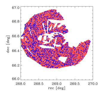
Figure 1: Position map of the MIR galaxy sample chosen by means of the Support Vector Machines algorithm (blue points). Red points mark the shape of the mask of the field

We estimate the completeness of the derived catalog empirically to be 150 $\mu$Jy, by defining the limit as a point of the maximum of the differential number counts of sources.

2.2 Redshift estimation

Since follow-up spectroscopic measurements are time consuming and, for the AKARI NEP Deep Field, the existing measurements are very sparse (which is addressed further in the text), and we have to rely on the photometric estimation of the redshifts. The usual photometric redshift estimation codes are based on fitting the abundance of optical templates for sources, like the LePhare routine (Ilbert et al., 2006). However, since the only measurements available for our sources are performed in the $NIR$ and $MIR$, we had to approach this task in an alternative way. To this aim, we ran the Code Investigating GALaxy Emission (CIGALE; Noll et al. 2009), a spectral energy distribution (SED) fitting routine. CIGALE was not developed as a tool for estimation of photo-$z$ but since it uses a large number of models covering the whole spectrum including IR, it may be expected to provide $z_{\mbox{\tiny{photo}}}$ using only the infrared part of spectra (Malek et al., 2012) with satisfactory quality. The CIGALE technique uses models describing the emission from a galaxy in the wavelength range from far-UV to far-IR. Models of emission from stars are given either by Maraston (2005) or Fioc & Rocca-Volmerange (1997). The absorption and scattering of star light by dust, the so-called attenuation curves for galaxies, are given by Calzetti et al. (2000). Dust emission is characterized by a model proposed by Dale & Helou (2002). In this model, the IR part of an SED is given by a power-law distribution

$${\rm d}M_{{\rm d}}(U)\propto U^{-\alpha_{{\rm SED}}}dU,$$ (2)

where $M_{\rm d}(U)$ is the mass of dust heated by a radiation field $U$, and $\alpha_{\rm SED}$ is a heating intensity.

To find a photometric redshift with CIGALE, it is necessary to shift a galaxy spectrum to many different redshifts and then to run CIGALE to fit SEDs for the same galaxy with a number of combinations of different redshift values. We decided to estimate photometric redshift for the AKARI NEP sample in the redshift range from $z_{\rm{min}}=0.01$ to $z_{\rm{max}}=3.00$ with a step $\delta z$=0.02. The final redshifts assigned by CIGALE are based on the minimal $\chi^{2}$ value of the fit with 7 degrees of freedom (for details, see Noll et al. 2009). In the same sample of 1339 galaxies, it was not possible to estimate photometric redshift ($\chi^{2}$ equal to $99.99$) for only 4.85 % of the sources. For 38.31 % of the galaxies, the $\chi^{2}$ was lower than 10.

The distribution of the $\chi^{2}$ is shown in Figure 2. The resultant redshift distribution obtained using CIGALE is presented in the Fig. 3, where it is compared to the other estimations previously published in the literature. The detailed description of the application of CIGALE to AKARI data is discussed at length in Małek et al. (2014).

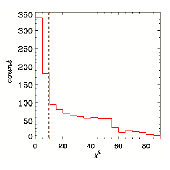
Figure 2: The distribution of the $\chi^{2}$ value obtained by redshift estimation analysis (shown in bins of 5.0). The vertical dashed line marks a cut at $\chi^{2}=10$, corresponding to the best SED fits used later for the analysis. Sources with $\chi^{2}$ values equal to 99.99 are not shown.

Previous studies of photometric redshift estimates of the 24 $\mu\mbox{m}$ selected sources have identified two peaks in the redshift distribution. Depending on the flux density limits, many studies have reported a rise in the detection of sources at $z<1$ peaking between $z\sim 0.3$ (e.g., Desai et al. 2008) and $z\sim 0.8$ (Pérez-González et al. 2005; Le Floc’h et al. 2005; Caputi et al. 2006). At these redshifts there are no prominent spectral features in the 24 $\mu\mbox{m}$ band except for the $\sim 16$ and 17 ${\rm\mu m}$ PAH emission bands. Some authors (e.g., Caputi et al. 2006) have reported that between the redshifts of $z\sim 0.8$ to $z\sim 1.6$ the number of detected 24 $\mu$m objects decreases significantly, possibly because of the deep silicate absorption line features at 9.7 $\mu\mbox{m}$ rest frame causing some sources to fall out of the flux detection limit. However, Desai et al. (2008) report a tentative detection of a distribution peak at $z\sim 0.9$, which has not been detected in previous studies. This distribution peak can be attributed to the 12.7 $\mu\mbox{m}$ PAH feature and 12.8 $\mu\mbox{m}$ [Neii] emission line, which at this redshift is seen in the 24 $\mu\mbox{m}$ passband.

An additional peak predicted by models (e.g., Lagache et al. 2004), which occurs at $z\sim 2$, can be attributed to sources dominated either by an AGN, or as a consequence of PAH emission features at $\sim$ 8$\mu\mbox{m}$ (e.g., Caputi et al. 2006).

The results of our photometric redshift derivation using the CIGALE code reveals results that are in agreement with these studies (see Fig. 3). We observed two expected peaks in the photo-$z$ distribution, one located at $z\sim 0.6$ and the weaker secondary peak located at $z\sim 1.2$. Moreover, we detect a noticeable rise in the counts at $z\sim 2.4$.

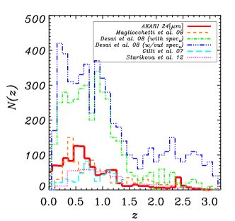
Figure 3: Redshift distribution of the AKARI NEP Deep Field MIR selected galaxies derived by CIGALE code (solid line) together with those published in the literature (dashed: Magliocchetti et al. 2008; dash-dot-dashed and dash-triple-dotted: Desai et al. (2008), for objects with and without spectroscopic redshifts; large-dashed: Gilli & Daddi 2007; and dotted: Starikova et al. 2012).

Murata et al. (2013) recently released a catalog with measurements of spectroscopic redshifts for a sample of 307 objects within the AKARI NEP Deep field obtained by DEep Imaging Multi-Object Spectrograph (DEIMOS) in Keck II telescope (Faber et al. 2003; Goto et al. in prep). Since the best way to estimate the accuracy of the photo-$z$ measurement procedure is to check it with directly measured spectroscopic redshifts, we have cross-correlated our catalog with that of Murata et al. (2013). We have found 149 counterparts from the spectroscopic catalog. Six of them resulted in CIGALE finding no believable redshift ($\chi^{2}>99$). To check the reliability of the photometric estimations we estimate the amount of the catastrophic errors (CE) for sources, following Ilbert et al. (2009). A CE occurs when the value of

$${\rm\eta=\frac{|z_{spec}-{\rm(photo-}z)|}{1+z_{spec}}}$$ (3)

exceeds $0.15$. We estimate this value for several limiting $\chi^{2}$ cuts to determine the value that is the most reliable for a clustering analysis. Figure 4 shows the comparison between the derived photometric redshifts and spectral measurements, whereas Table 1 presents the results of this procedure. The amount of the CE reaches $18.37\%$ for $\chi^{2}<10$ and then increases significantly with the increase of the $\chi^{2}$ value until it reaches a value of almost twice as high for the $\chi^{2}<70$.

Table 1: Comparison of ${\rm z_{CIGALE}}$ vs ${\rm z_{spec}}$ as a function of $\chi^{2}$. $\eta$ - percent of CE in the sample.

$\chi^{2}$	${\rm N_{gal}}$	${\rm N_{CE}}$	$\eta$ [%]
70	126	44	34.92
50	112	39	34.82
30	73	21	28.77
20	65	18	27.69
10	49	9	18.37

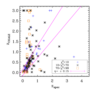
Figure 4: Comparison between $z_{\rm{CIGALE}}$ and $z_{\rm{spectro}}$. Different symbols correspond to different $\chi^{2}$ values: blue crosses denote objects with $\chi^{2}<10$, black asterisks objects with $10\leq\chi^{2}<70$, and orange squares objects with $70\leq\chi^{2}<99$. Solid lines are for $z_{\rm{CIGALE}}=z_{\rm{spectro}}\pm 0.15(1+z_{\rm{spectro}})$.

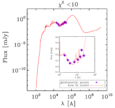
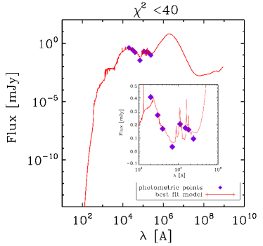
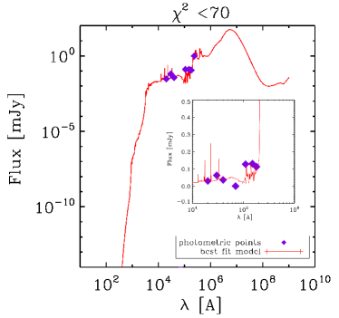
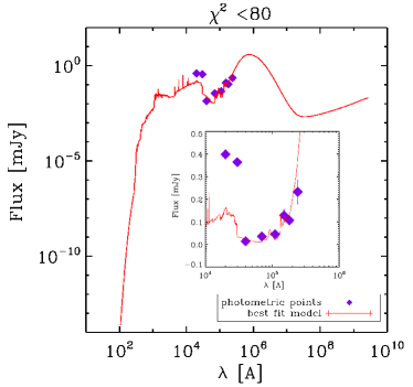
Figure 5: Examples of the CIGALE fitted SED’s to the AKARI NEP Deep data for different $\chi^{2}$ values. Each plot has a close-up on the photometric data in the linear scale.

In Fig. 5 we present the examples of the resultant SEDs obtained with different $\chi^{2}$ values. It is clear that for values from $\chi^{2}\sim 40$ up to the $70$ we are still dealing with the very good fits to the data. The fits with values of $\chi^{2}\sim 80$ no longer seem reliable. The redshift distributions of the sources included within a specific $\chi^{2}$ cut are presented in Fig. 6.

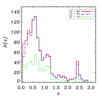
Figure 6: The redshift distribution of the AKARI NEP Deep sources obtained by the CIGALE code as a function of the limiting $\chi^{2}$ value. Distribution of all sources, with a successfully calculated $z_{\rm photo}$ is represented by the solid line, distribution of sources with photometric redshift measurements on the level of $\chi^{2}<10$ by dash-dotted line, and $\chi^{2}<70$ by dash-triple-dotted line.

For the most reliable results, we decided to replace the photometric redshifts for objects that have a spectroscopic measurement from the Murata et al. catalog, and assigned them the value of $\chi^{2}=0$. This procedure increased the number of sources from 511 to 611 for the ${\rm\chi^{2}<10}$ sample, from 1195 to 1220 for the ${\rm\chi^{2}<70,}$ and from 1268 to 1274 for the full catalog without the galaxies for which the CIGALE code was unable to retrieve the redshift.

3 The angular correlation function

Galaxy clustering is traditionally analyzed in the first place by the means of the two-point correlation function, $\xi(r)$, which is treated as an above random excess probability of finding a galaxy within a certain distance $r$ from another galaxy. Often it is approximated by a power law $\xi(r)=(r/r_{0})^{(-1/\gamma)}$.

3.1 Estimator

To compute the angular correlation function, we use the following estimator introduced by Landy & Szalay (1993):

$${\rm\omega(\theta)=\frac{DD(\theta)-2DR(\theta)+RR(\theta)}{RR(\theta)}}$$ (4)

where ${\rm DD(\theta)}$ is the number of galaxy-galaxy pairs, ${\rm RR(\theta)}$ is the number of random-random pairs, and ${\rm DR(\theta)}$ is the number of galaxy-random pairs within an angular bin of separation on the sky ${\rm\theta}$.

We use $10^{5}$ homogeneously generated random points within the FOV and overlay the photometric mask with the identical features as the real FOV. Because of the masking of bad sectors of the FITS file for the 24 $\mu\mbox{m}$ passband, the effective number of galaxies used for the calculation was significantly reduced (by $\sim 36$ % of the original number of sources). The correlation function was computed in the angular bins of width $\delta\log\theta=0.1$.

3.2 Errors

The uncertainties arising from computation of the correlation function through the Landy-Szalay estimator are

$${\rm\delta\omega(\theta)=\frac{1+\omega(\theta)}{\sqrt{DD(\theta)}},}$$ (5)

which accounts for the standard deviation in the pair counting along with the intrinsic variance. However it does not include the error arising from the covariance of the correlation function at different separations. There are a number of ways to avoid this problem; for instance, using bootstrap resampling of the data (e.g., Barrow et al. 1984 ), mock catalogs (e.g., Pollo et al. 2005), jackknife resampling (e.g., Gaztanaga 1994; Ross et al. 2007; Scranton et al. 2002), and many others. We employ the jackknife resampling of the data to calculate errors. To this aim we divided the observed field into ten equally sized areas and computed the correlation function ten times, each time leaving one area out. Then, the errors were estimated from Eq. 6,

$${\rm\sigma^{2}=\sum_{i=1}^{10}[\omega_{i}(\theta)-\omega(\theta)]^{2},}$$ (6)

where $i$ denotes a particular subsample iteration. We calculated all presented uncertainties from here on in this manner.

3.3 Fitting procedure and integral constraint

Usually a correlation function follows the power law

$${\rm\omega(\theta)=A_{\omega}(\theta^{\bf{1-\gamma}}),}$$ (7)

(e.g., Peebles 1994). Every estimate of ${\rm\omega({\theta})}$ is penalized by the finite size of the surveyed area and referred to as the ”integral constraint” (IC, Peebles & Groth 1976). This effect causes a negative offset of the observed ${\rm\omega(\theta)}$ with respect to the true correlation function, ${\rm\omega_{T}(\theta)}$, by a constant

$${\rm IC=\int\int\omega_{T}(\theta)d\Omega_{1}d\Omega_{2},}$$

where ${\rm d\Omega_{1}}$ and ${\rm d\Omega_{2}}$ are the transverse solid angles of each pair. It can be approximated using the following formula:

$$IC=\frac{\Sigma RR(\theta)\omega(\theta)}{\Sigma RR(\theta)},$$ (8)

introduced by Roche & Eales (1999). After applying this correction, the correlation function can be written as ${\rm\omega(\theta)=A_{\omega}(\theta^{\bf{1-\gamma}}-IC)}$. To determine the best-fit parameters ($\gamma$, $A$), we performed a ${\rm\chi^{2}}$ minimization including the full covariance matrix $C$, i.e.,

$${\rm\chi^{2}=[\omega(\theta)-(A_{\omega}\theta^{{\bf 1-\gamma}}-IC)]^{T}C^{-1}[\omega(\theta)-(A_{\omega}\theta^{\bf{1-\gamma}}-IC)].}$$

3.4 Limber inversion and space clustering

Using the measurements of the angular clustering, we can infer the three-dimensional clustering properties based on the known redshift distribution via Limber’s equation (Peebles 1980, Limber 1953). When dealing with small scales both angular and spatial correlation functions are well described by power laws (e.g., Davis & Peebles 1983) and therefore Limber’s equation can be presented in the form (Efstathiou et al. 1991),

$${\rm A_{\omega}=C_{\gamma}r_{0}^{\gamma}\frac{\int d_{A}^{1-\gamma}x^{-1}(z)(dN/dz)^{2}dz}{[\int(dN/dz)]^{2}}},$$ (9)

where $d_{A}$ is the angular diameter distance, $x(z)$ is the derivative of proper distance with redshift,

$$C_{\gamma}=\frac{\sqrt{\pi}\Gamma(\frac{\gamma-1}{2})}{\Gamma(\gamma/2),}$$ (10)

and dN/dz is the redshift selection function, which in case of our study is derived empirically from SED fitting (see Fig. 3).

3.5 Galaxy bias

In order to relate galaxy clustering to dark matter clustering, Kaiser (1984) and Bardeen (1986) introduced a bias parameter, a quantity describing the differences between the clustering of a galaxy field and the underlying mass distribution, i.e.,

$$b^{2}(r,z,M)=\xi_{g}(r,z,M)/\xi_{m}(r,z),$$ (11)

where $\xi_{g}(r,z,M)$ is the correlation function of the investigated galaxy population, and $\xi_{m}(r,z)$ is the correlation function of the dark matter. Bias is dependent on scale ($r$), redshift ($z$) and objects’ mass ($M$). In terms of the assumed fluctuations of mass traced by galaxies (${\rm\sigma_{g}}$) and mass ($\sigma_{m}$), the bias parameter should satisfy the relation

$$\rm{\sigma_{(g,R)}=b\sigma_{(m,R)}}.$$ (12)

It can be presumed that $b$ is invariant as long as the scales are large enough. In this case it is customary to compute $\sigma_{R}$ for a representative scale $R=$8 ${\rm h^{-1}}$Mpc (Quadri, 2007). To obtain the value of ${\rm\sigma_{(m,8)}}$ for different cosmic epochs, one can use a following formula:

$$\rm{\sigma_{(m,8)}(z)=\sigma_{(m,8)}(0)D(z),}$$ (13)

where $\sigma_{(m,8)}(0)$ is a present day ($z=0$) mass fluctuation, which on the scale $R$ of 8 $h^{-1}$Mpc has a value of 0.83 (Planck Collaboration et al., 2014); and

$$\rm{D(z)=\frac{g(z)}{g(0)(1+z)},}$$ (14)

where $g(z)$ is a normalized growth factor that describes the growth rate of the matter density fluctuations, and can be calculated, according to Carroll et al. (1992), as follows:

$$g(z) \sim\frac{5}{2}\Omega_{m}(z)[\Omega_{m}^{4/7}(z)-\Omega_{\Lambda}(z)+$$ (15)

$$+\left(1+\frac{\Omega_{m}(z)}{2}\right)\left(1+\frac{\Omega_{\Lambda}(z)}{70}\right)]^{-1}.$$

The value of the fluctuations of the galaxy density ($\sigma_{g,8}$) with respect to the assumed scale can be obtained by implementation of the correlation function slope $\gamma$ and correlation length $r_{0}$, i.e.,

$${\rm\sigma_{g,8}=\sqrt{J_{2}\left(\frac{r_{0}}{8h^{-1}Mpc}\right)^{\gamma}},}$$ (16)

where $J_{2}=72/(2^{\gamma}(3-\gamma)(4-\gamma)(6-\gamma)).$

4 Results

Following the procedures described in the previous subsections we compute ${\rm\omega({\theta})}$ for the 24 ${\rm\mu\mbox{m}}$ selected galaxy catalog. The angular distances were measured in bins of ${\rm\Delta\mbox{log}=0.2}$. We then fitted the data using a $\chi^{2}$ technique with $2\sigma$ clipping and determined the errors from the covariance matrix.

The results of the power-law fitting to the correlation function between the full catalog (with ${\rm\chi^{2}>99}$) and subcatalog of the best redshift quality (${\rm\chi^{2}<10}$) show, that the two samples differ significantly. The full catalog showed $r_{0}=4.93\pm 0.49$ $h^{-1}\mbox{Mpc,}$ while the subcatalog showed $r_{0}=6.47\pm 0.56$ $h^{-1}\mbox{Mpc}$.

The low $r_{0}$ value for the sample containing all $\chi^{2}$ values but the failing ones could be a result of the fact that it contains galaxies with lower fluxes, which would dilute the clustering signal.

The difference is significant between the fit values for the subsamples with $\chi^{2}$ smaller then 10 and the full catalog. Depending on the $\chi^{2}$ cut we see drastic changes in both the strength and in the slope of the clustering.

The most secure galaxies (with redshift estimation on the level of $\chi^{2}<10$) exhibit a much larger correlation length when compared with the whole sample. The $\chi^{2}<10$ galaxies are concentrated around $z\sim 0.7$ (dash-dotted line on Fig. 6). The brightness distribution of those sources reveals that this sample consists mostly of the objects with ${\rm S_{24\mu m}}>500$ $\mu$Jy. This result could indicate that galaxies with the most secure redshifts are the most luminous objects within the AKARI sample. In the following analysis, we only focus on this subsample of galaxies. We present the 24 $\mu$m flux as a function of redshift for the $\chi^{2}<10$ sample in Fig. 7.

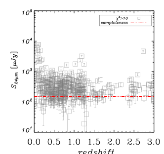
Figure 7: 24 $\mu$m flux of objects from $\chi^{2}<10$ sample as a function of their redshift. The flux limit, marked as a red line, was derived from maximum of differential number counts of detected sources.

4.1 High- and low-redshift population sample

The galaxies with a successfully calculated $z_{\rm CIGALE}$ on the goodness of fit level of $\chi^{2}<10$ were divided into four redshift ranges based on the shape of resultant distribution: 1) the low-$z$ sample composed of sources with $z\leq 0.5$; 2) the low-intermediate sample with $0.5<z\leq 0.9$, which includes the primary and most evident peak of the distribution which, as stated before, could be a result of 16.3 ${\rm\mu m}$ and/or 17 ${\rm\mu m}$ PAH emission features passing through 24 $\mu$m passband; 3) the intermediate sample with $0.9<z\leq 1.3,$ including the secondary peak attributed to the 12.7 ${\rm\mu m}$ PAH and/or 12.8 ${\rm\mu m}$ [Neii] emission features, which at these redshifts would pass through the 24 ${\rm\mu m}$ passbands; and 4) the high-$z$ sample with $z>1.3$, a range, which includes the possible peak at $z\sim 2.4$ in which we expect a significant incompleteness since sources could fall out of the detection limits due to the deep silicate absorption features at $\sim$ 9.7 ${\rm\mu m}$. At $z\sim 1.5,$ these features would appear in $\sim$24 ${\rm\mu{\rm m}}$ passbands. For the subsamples divided in this way, we estimated the angular correlation function. What is more, as a by-product of the photometric redshift estimation we were able to obtain the estimates of the $L_{TIR}$ for the galaxies in the AKARI 24 $\mu$m selected sample. The details of the analysis of the physical parameters for the sources from AKARI NEP Deep Field using CIGALE will be addressed in Malek et. al (in prep) and Buat et al. (in prep). Here we use the output for general purposes only.

Fig. 8 shows the results of this calculation, while the Table 2 lists the derived power-law fitting parameters along with the corresponding correlation lengths, $L_{TIR}$, and bias (see subsection 4.2) for galaxies in each redshift bin. Table 3 summarizes the amount of the catastrophic errors obtained within each considered redshift range.

For the lowest redshift interval ($z\leq 0.5$), which predominantly contains galaxies with total infrared (TIR) luminosities of an order of $10^{10}L_{\odot}$, the derived correlation length is equal to $3.62\pm 0.79h^{-1}\mbox{ Mpc}$. At redshifts $0.5<z\leq 0.9,$ we start to observe a LIRG population ($L_{TIR}\sim 10^{11}L_{\odot}$), which displays a higher $r_{0}$: $6.21\pm 0.78h^{-1}\mbox{ Mpc}$ and mean $L_{TIR}$$\sim 1.4\cdot 10^{11}L_{\odot}$.

The higher-$z$ population ($0.9<z\leq 1.3$) displays a correlation length ($r_{0}=5.86\pm 0.69$ $h^{-1}\mbox{ Mpc}$) similar to that of the lower-z population, however, it displays a significantly higher $L_{TIR}:\sim 7\cdot 10^{11}L_{\odot}$. The correlation function of galaxies in the $z>1.3$ has a correlation length of $7.23\pm 0.87\mbox{ Mpc}\mbox{ }h^{-1}$. Even though this sample has the largest redshift dispersion, the clustering signal is not a subject to any substantial dilution. Nevertheless, the amount of the catastrophic errors within this bin is high ($\sim 83\%$, see Table 3); therefore without any additional follow-up measurements of redshifts to confirm our results, conclusions based on this bin cannot be reliable.

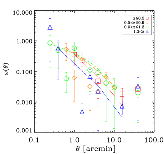
Figure 8: Two-point angular correlation function calculated for the subsamples divided according to the derived photometric redshifts with $\chi^{2}<10$. Squares represent the low z sample ($z\leq 0.5$), diamonds a sample with $0.5<z\leq 0.9$, circles the sample with $0.9<z\leq 1.3,$ and triangles the high z sample with $z>1.3$.

Table 2: Clustering of 24 $\mu$m galaxies in AKARI NEP Deep Field.

$\chi^{2}$	$z$ range	${\rm N_{gal}}$	${\rm\gamma}$	$r_{0}\mbox{ }[h^{-1}\mbox{Mpc }]$	$L_{TIR}$	b
10	$z\leq 0.5$	168	$1.99\pm 0.06$	$3.62\pm 0.76$	$10.276\pm 0.81$	$0.89\pm 0.20$
10	$0.5<z\leq 0.9$	207	$1.69\pm 0.03$	$6.21\pm 0.78$	$11.15\pm 0.315$	$1.72\pm 0.25$
10	$0.9<z\leq 1.3$	159	$1.57\pm 0.10$	$5.86\pm 0.69$	$11.84\pm 0.36$	$1.91\pm 0.21$
10	$z>1.3$	77	$1.85\pm 0.12$	$7.23\pm 0.87$	$12.43\pm 0.44$	$3.53\pm 0.51$

Table 3: Comparison of $z_{\rm CIGALE}$ vs $z_{\rm spec}$ as a function of $\chi^{2}$. $\eta_{\rm{bin}}$ - percent of CE in the redshift bin, $\eta_{\rm{tot}}$ - percent of CE in the total matched sample.

$\chi^{2}$	$z_{\rm range}$	$N_{\rm gal}$	$N_{\rm CE}$	$\eta_{\rm{bin}}$ [%]	$\eta_{\rm{tot}}$ [%]
10	$z\leq 0.5$	32	0	0.00	0.00
10	$0.5<z\leq 0.9$	5	1	20.00	1.92
10	$0.9<z\leq 1.3$	6	3	50.00	5.77
10	$1.3<z$	6	5	83.33	9.62

4.2 Galaxy bias

We study the bias $b$ of the 24 $\mu$m selected AKARI galaxies as described in subsection 3.5. We leave a more detailed study using a full Halo Occupation Distribution (HOD, Scoccimarro et al. 2001) formalism for future work.

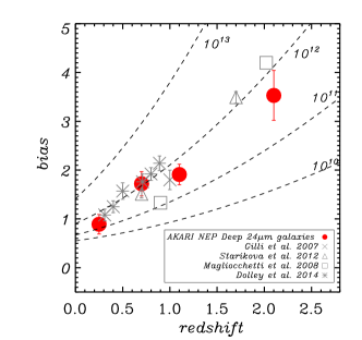
Figure 9: Linear bias as a function of redshift for AKARI photometric redshift samples (filled circles). Dashed curves represent the theoretical linear halo bias evolution of dark matter halos of minimal masses: $10^{10}$, $10^{11}$, $10^{12}$, and $10^{13}$ (from bottom to top). As a reference we show results from the literature: triangles mark results from Starikova et al. (2012), squares the results from Magliocchetti et al. (2008), crossesthe results from Gilli & Daddi (2007), and asterisks from Dolley et al. (2014).

Once the bias factors have been computed for all AKARI galaxy subsamples (section 3.5), it is possible to trace their evolution with redshift. This procedure can give an insight into what kinds of galaxies the 24 $\mu$m selected samples could correspond to at the current epoch: $z=0$ (Nusser & Davis 1994, Moscardini et al. 1998). This approach is however simplified: it is based on the assumption that galaxies throughout their evolution do not interact with each other and they are only influenced by their density field. We can track the evolution by the relation, i.e.,

$$b(z)=1+\frac{b(0)-1}{D(z)},$$ (17)

where ${\rm D(z)}$ is given by eq. 14, and $b(0)$ is a value of bias at $z=0$.

In Fig. 9 we show the linear bias evolution derived from Sheth & Tormen (1999) formalism for varying minimum dark matter halo (DMH) mass thresholds. The minimum masses of DMH for galaxies within redshift intervals of $z<0.5$ and $0.9<z\leq 1.3$ are located between $10^{11}M_{\odot}h^{-1}<M_{h}<10^{12}M_{\odot}h^{-1}$. For $0.5<z\leq 0.9$ interval, galaxies are expected to have a slightly higher minimum mass than other considered samples: $10^{12}M_{\odot}h^{-1}\geq M_{h}$. However, since values of bias parameters for the intervals of $0.5<z\leq 0.9$ ($b=1.72\pm 0.25$) and $0.9<z\leq 1.3$ ($b=1.91\pm 0.21$) are in agreement within their error bars, this result for the lower $z$ sample could be misleading. Nevertheless, if it is a true effect, it could indicate that IR galaxies with higher $L_{TIR}$ do not necessarily reside in more massive DMHs, as in the case of redshift intervals of $0.9<z\leq 1.3$ (with $L_{TIR}\sim 7\cdot 10^{11}L_{\odot}$) and $0.5<z\leq 0.9$ (with $L_{TIR}\sim 1.4\cdot 10^{11}L_{\odot}$). This idea is consistent with the work of Goto (2005), where it has been reported (for the IR galaxies observed by IRAS) that more IR luminous galaxies tend to have smaller local density. They argue that luminous infrared galaxies with moderate total infrared luminosities ($10^{10.5}L_{\odot}<L_{TIR}<10^{11}L_{\odot}$) exist in higher density regions than IR galaxies with $10^{11}L_{\odot}<L_{TIR}<10^{12}L_{\odot}$. Therefore there must exist a discrepancy in the origin of these two potentially different populations. If LIRGs are created through a merger and/or interaction of several galaxies (e.g., Taniguchi et al. 1998, Borne et al. 2000), then their local environment would naturally be lower. Then, the higher minimal DMH of the AKARIs’ $0.5<z\leq 0.9$ could mean that within this interval we still observe a substantial fraction of normal spiral galaxies in addition to interacting systems. It has been reported that up to $z\sim 0.5-0.7$ more than a half of the LIRG population is composed of normal spiral galaxies (Bell et al. 2005; Melbourne et al. 2005; Elbaz et al. 2007). Beyond those redshifts, mergers start to enhance the $L_{TIR}$ and deplete the environment. However, a relatively large $r_{0}$ of AKARIs’ galaxies is contradictory to local measurements of clustering lengths of star-forming spiral galaxies ($r_{0}\sim 4$ $h^{-1}{\rm Mpc}$; e.g., Coil et al. 2004; Meneux et al. 2006; Coil et al. 2008; Heinis et al. 2009). On the other hand, AKARI NEP Deep survey is flux limited, therefore, at larger redshifts it preferentially and intrinsically detects more luminous galaxies, which in turn are more strongly clustered. This could result in an increase of the measured $r_{0}$ in this redshift range. This issue remains undetermined and a more detailed analysis of those galaxies is needed to determine their true nature, which is a subject of future research.

With known $b(z)$, we can trace the evolution of $\xi_{g(r=8,z)}$, and therefore the evolution of the $r_{0}(z)$, by inverting Eq. 11. This procedure can lead to the determination of a possible fate of each considered population.

The results are shown in Fig. 10. AKARI 24 $\mu$m galaxies at $z_{med}=0.25$ exhibit a steep correlation function slope ($\gamma\sim 2$) and a correlation length of $3.62\pm 0.76$ $h^{-1}{\rm Mpc}$. Their evolution with time could result in reaching $r_{0}\sim 4$ $h^{-1}{\rm Mpc}$ at the present day. Therefore, according to those measurements, the majority of the AKARI galaxies at low-z are expected to fall into this category.

The galaxies within redshift ranges of $0.5<z\leq 0.9$ and $0.9<z\leq 1.3$ could evolve into a very strongly clustered population of galaxies, with $r_{0}\sim$ 8-8.5 $h^{-1}{\rm Mpc}$. In the local Universe, early type galaxies with $L\sim L_{*}$ have been measured to have similar correlation lengths: $r_{0}\sim 8$ $h^{-1}{\rm Mpc}$ (Guzzo et al. 1997). This means that those objects could have evolved from the population of LIRGs at redshifts $\sim 0.9$. However, the slope of the clustering of AKARI galaxies ($\gamma\sim 1.65$) is lower than that measured for the local ellipticals ($\gamma\sim 2$).

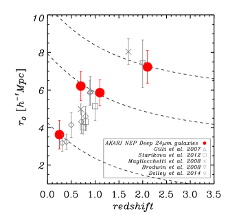
Figure 10: Correlation length of AKARI NEP Deep galaxies (red filled circles) compared with the evolutionary tracks as expected from the linear scenario (dashed lines). Triangles denote results from Gilli & Daddi (2007), squares from Starikova et al. (2012), crosses from Magliocchetti et al. (2008), reversed triangles from Brodwin et al. (2008), and diamonds from Dolley et al. (2014).

4.3 Comparison with previous studies

Figures 9 and 10 present a comparison of our derived spatial correlation lengths and biases for the redshift divided samples with the results from the literature.

As mentioned in Section 1, several previous studies have approached the task of analyzing the 24 ${\rm\mu\mbox{m}}$ selected galaxies by dividing the samples based on their redshift measurements. A direct comparison with previous studies is not a straightforward procedure because of the varying survey sizes and depths, different methods used to select the galaxy samples, and the difference in the considered redshift ranges. We present the first non-Spitzer based measurement of clustering of 24-$\mu$m selected sources. Table 4 shows a comparison of the previously investigated surveys of 24 $\mu$m selected galaxies throughout the literature.

Table 4: Summary and comparison of the previous 24 $\mu$m selected galaxy surveys. The work of Gilli & Daddi (2007) is based on spectroscopic measurements in contrast with other studies (based on photometric measurements).  The parameter $\rho$ stands for surface density.

	depth [$\mu$Jy]	$\rho^{}$ [${\rm N}_{{\rm gal}}/deg^{2}$]	size [$deg^{2}$]	probed $z$	$\gamma$	$r_{0}[\mbox{ }h^{-1}\mbox{Mpc}]$
Gilli & Daddi 2007	20	13060	0.1	$\sim 1$	$1.5\pm 0.1$	$4.0\pm 0.4$
Magliocchetti et al. 2008	400	1490	0.7	[0.6-1.2] & $<1.6$	–	$5.95_{-1.26}^{+1.10}$& $11.13_{-2.38}^{+2.03}$
Starikova et al. 2012	310	410	49	$\sim 0.7$ & $\sim 1.7$	1.8	$4.98\pm 0.28$&$8.04\pm 0.69$
Dolley et al. 2014	223	2678	8.42	$0.2<z<1.0$	$1.8-2.13$	$3-6$
AKARI	150	3350	0.4	$[0:3)$	$1.79\pm 0.04$	$4.93\pm 0.49$

It is worth noting that the source selection, which we have relied upon for this analysis, was based on the rough spectral shape of the considered sources. This excludes the possibility of mixing AGN dominated galaxies, in contrast with samples chosen without this kind of criterion.

Measurements of the correlation length of local ($0.3<z<0.6$) blue galaxies have been reported in several previous studies to be on the order of $\sim 3.7$ $h^{-1}{\rm Mpc}$ (e.g., Coil et al. 2004). This was found to be in agreement with the measurements of the rest-frame selected UV galaxies (see Milliard et al. 2007, Heinis et al. 2009). Since this value is consistent with that measured for the lowest-z AKARI galaxy subsample ($r_{0}=3.62\pm 0.76$ $h^{-1}{\rm Mpc}$), it could mean that it is mainly composed of the local, normal SF galaxies. The study by Masci & SWIRE Team (2006) for 24 $\mu$m selected galaxies in SWIRE survey found similar values of $r_{0}$: $3.32\pm 0.19$ $h^{-1}{\rm Mpc}$ with the steep slope $\gamma\sim 2$.

For the sample of $\sim$ 1300 objects ($S_{24\mu\mbox{m}}>20\mbox{ }\mu\mbox{Jy}$) with an average $L_{\rm IR}\sim 4\cdot 10^{10}L_{\odot}$ within the GOODS fields with $z_{med}\sim 0.8$, Gilli & Daddi 2007 have found the correlation length equal to $r_{0}=4.0\pm 0.4$ $h^{-1}{\rm Mpc}$. They have found that for LIRGs ($L_{\rm IR}>10^{11}L_{\odot}$) $r_{0}$ rises up to $5.14\pm 0.76$ $h^{-1}{\rm Mpc}$. These values are in agreement with that obtained for the LIRGS found in AKARI NEP-Deep survey.

The analysis performed by Magliocchetti et al. 2008 for 1041 galaxies brighter than $S_{24\mu{\rm m}}=400$ $\mu\mbox{Jy}$ resulted in obtaining the correlation lengths for low-$z$ ($z_{\rm mean}\sim 0.8$) and high-$z$ ($z_{\rm mean}\sim 2$) sources to be equal to $r_{0}=5.95^{+1.10}_{-1.26}$ $h^{-1}{\rm Mpc}$ and $r_{0}=11.13^{+2.03}_{-2.38}$ $h^{-1}{\rm Mpc}$, respectively. The value obtained for the low-$z$ sample, $z=[0.6-1.2]$, is comparable with that derived in this work ($r_{0}=5.86\pm 0.69$ $h^{-1}{\rm Mpc}$) for $0.9<z\leq 1.3$ range. This evidence for both studies at these redshifts points to the fact that they trace a population of galaxies that could evolve into present day $r_{0}\sim 8$ $h^{-1}{\rm Mpc}$ objects (possibly ellipticals with $L\sim L_{*}$).

The study by Starikova et al. 2012, based on Spitzer Wide-Area Survey within the SWIRE Lockman Hole field for more than 20000 objects brighter than $S_{24\mu{\rm m}}>310$ $\mu\mbox{Jy,}$ has shown that the correlation length for the low- ($z_{mean}\sim 0.7$) and high-$z$ ($z_{\rm mean}\sim 1.7$) samples are $r_{0}=4.98\pm 0.28$ ${\rm Mpc}$ ${\rm h^{-1}}$ and ${\rm r_{0}=}8.04\pm 0.69$ ${\rm Mpc}$ ${\rm h^{-1}}$, respectively. Our derived values for $0.5<z\leq 0.9$ are slightly higher ($r_{0}=6.21\pm 0.78$ $h^{-1}{\rm Mpc}$). The divergence of the results could arise because the widths of redshift intervals that are being compared are different. The low-redshift interval of Starikova et al. covers a range from $\sim 0$ to 2, with the mean $z\sim 0.7$. In AKARI’s range for $z_{median}\sim 0.7,$ we have not included the galaxies at $z$ lower than 0.5.

Furthermore, the recent study by Dolley et al. (2014) from the Spitzer observations of the Boötes field of over 22 000 24 $\mu$m galaxies up to $z\sim 1$ shows correlation lengths varying with redshift, from $r_{0}\sim 3$ to $r_{0}\sim 6$ $h^{-1}{\rm Mpc}$. Subsamples at $z_{median}\sim 0.3$ with $r_{0}=3.18\pm 0.44$ $h^{-1}{\rm Mpc}$ and $z_{median}\sim 0.9$ with $r_{0}=5.86\pm 0.66$ $h^{-1}{\rm Mpc}$ show a good agreement with our results at similar median redshifts: $r_{0}=3.62\pm 0.76$ $h^{-1}{\rm Mpc}$ at $z_{median}\sim 0.25$ and $r_{0}=6.21\pm 0.78$ $h^{-1}{\rm Mpc}$ at $z_{median}\sim 0.7$.

It is also worth noting that the subsample of AKARI galaxies with the highest $z$ indicates a correlation length value ($r_{0}=7.23\pm 0.87$ $h^{-1}{\rm Mpc}$ ), which is consistent with the work of Brodwin et al. (2008). Their investigation was focused on clustering analysis of $\sim 2600$ dust obscured galaxies (DOG) with spectroscopic redshifts located at $1.5<z<2.5$. A detection of strong clustering with $r_{0}=7.4^{+1.27}_{-0.84}$ $h^{-1}{\rm Mpc}$ for a ${\rm S_{24\mu m}}>$ 300 $\mu$Jy flux cut was reported. However, these values from the AKARI analysis were derived from small number statistics, and therefore, these results should be treated with caution.

5 Summary and conclusions

We have presented a clustering analysis of the $S_{24\mu{\rm m}}$ selected AKARI NEP Deep field galaxies down to a flux limit of 150 $\mu$Jy. This is the first study of these kinds of sources that are not based on Spitzer telescope measurements and features a source selection that does not rely on any auxiliary observations from other wavelength intervals.

After performing the sample selection through the use of the SVM classifiers trained on the infrared color information, we used the CIGALE code to estimate the photometric redshifts for the chosen galaxies, and we were able to establish a redshift estimate for 96.11 % of the sample. The resultant redshift distribution revealed three peaks: the primary one located at $z\sim 0.6$, which can be attributed to either the evolution in the luminosity function or to the increase of the detection volume; a secondary peak located at $z\sim 1.2$ possibly related to the $12.7$ and 12.8 $\mu$m PAH emission lines passing through the 24 $\mu$m passband at these redshifts; and an indication of a possible third peak at $z\sim 2.4$. Even though AKARI’s high-z peak is too tentative to draw any firm conclusions about any possible population of galaxies, several models predict its existence and attribute it to the sources dominated either by AGNs or by a PAH emission feature at 8 $\mu$m.

For the calibration of those measurements, we have compared them with the spectroscopic redshifts for counterparts available from Murata et al. catalog (149 objects) and estimated that, depending on the goodness of fit value, we encounter a 18.75 % rate of CE for $\chi^{2}<10$ and 35.22 % for $\chi^{2}<70$. Therefore, the following clustering analysis was performed only on a subsample of galaxies with the most secure redshift estimation. To obtain the most reliable results, we substituted the photometric redshift measurements for the objects possessing the spectroscopic redshift measurements. With a set of galaxies prepared in the way described above, we examined the clustering properties of the derived samples with respect to their redshift distribution.

Using a power-law approximation to derive correlation function together with the estimated photometric redshift information, we obtained the spatial correlation length $r_{0}$. For the full sample, the derived value equals $r_{0}=4.93\pm 0.49$ $h^{-1}{\rm Mpc}$, which is consistent with the previous studies conducted for the same wavelengths. For the specific redshift intervals we have found the following facts:

1. For $z\leq 0.5$ $r_{0}=3.62\pm 0.79$ $h^{-1}\mbox{ Mpc}$, $L_{TIR}$ $\sim 10^{10}L_{\odot}$. This indicates that this redshift interval is mostly composed of normal SF galaxies. Their bias parameter is equal to $0.93\pm 0.11$ and their estimated minimal DMH mass is $M_{h}>10^{11}M_{\odot}$.

2. For $0.5<z\leq 0.9$ and $0.9<z\leq 1.3$:

   • correlation lengths are $6.21\pm 0.78$ $h^{-1}\mbox{ Mpc}$ and $5.86\pm 0.69$ $h^{-1}\mbox{ Mpc}$, respectively ;

   • galaxies exhibit very similar, relatively high values of bias parameter ($\sim 1.7-1.9$). Those values are consistent with the linear bias derived in work of Lagache et al. (2007), which was measured from Cosmic Far-Infrared Background anisotropies at 160 $\mu$m ($b=1.74\pm 0.16$). Both measurements probe similar redshift range ($z_{Lagache}\sim 1$).

   • the sample at $0.9<z\leq 1.3$, composed of brighter galaxies ($L_{TIR}\sim 10^{11.84}L_{\odot}$), seems to be residing in lower minimal mass DMH ($M_{h}<10^{12}M_{\odot}h^{-1}$) than the lower luminosity (with $L_{TIR}\sim 10^{11.15}L_{\odot}$ and $M_{h}>10^{12}M_{\odot}h^{-1}$) galaxies at $0.5<z\leq 0.9$. This could indicate that brighter infrared galaxies do not necessarily reside in more massive halos. This means that despite similar clustering properties, we are dealing with two different populations of star-forming galaxies. The redshift distribution shows two distinct peaks (at $\sim 0.6$ and $\sim 1.2$): the primary peak in the redshift distribution at $\sim 0.6$ could contain a mix of both normal star-forming galaxies and LIRGs. The dip in the distribution between the peaks at $\sim 0.9$ could mean that normal galaxies slowly fade out from the field of view to reveal a more prominent LIRG population at redshifts $\sim 0.9$ and higher.

   • Extrapolating the AKARI data to the present day epoch has allowed us to investigate the approximate descendants of each galaxy subsample. Working under the assumption that galaxy interactions do not affect the $\sigma_{m}$ value at scales as large as 8 Mpc, 24 $\mu$m galaxies at redshifts $0.5<z<1.3$ could evolve into current galaxies with $r_{0}\sim 8$ $h^{-1}{\rm Mpc}$, a value measured for ellipticals with $L\sim L_{*}.$

3. Galaxies at $z>1.3$ display a strong clustering signal at small scales despite the large size of the redshift range. This could indicate an existence of separate, highly clustered population(s). However, because of small number statistics burdened with a large number of CE, these results remain unconfirmed.