Muonic hydrogen as a quantum gravimeter

Abstract

High precision spectroscopy of muonic hydrogen has recently led to an anomaly in the Lamb shift, which has been parametrized in terms of a proton charge radius differing by seven standard deviations from the CODATA value. We show how this anomaly may be explained, within about a factor of three, in the framework of an effective Yukawian gravitational potential related to charged weak interactions, without additional free parameters with respect to the ones of the standard model. The residual discrepancy from the experimental result in this model should be attributable to the approximations introduced in the calculation, the uncertainty in the exact value of the Fermi scale relevant to the model and the lack of detailed knowledge on the gravitational radius of the proton. The latter cannot be inferred with electromagnetic probes due to the unknown gluonic contribution to the proton mass distribution. In this context, we argue that muonic hydrogen acts like a microscopic gravimeter suitable for testing a possible scenario for the reciprocal morphing between macroscopic gravitation and weak interactions, with the latter seen as the quantum, microscopic counterpart of the former.

I Introduction

Precision studies of the hydrogen spectroscopy have played a major role in shaping our knowledge of the microscopic world and its understanding in terms of quantum mechanics and quantum field theory Reviewspectroscopy . Precision spectroscopy of hydrogen has now reached a point where the accuracy in the comparison to quantum electrodynamics is limited by the proton size, in the form of the root-mean square (rms) charge radius, $r_{p}=\langle r_{p}^{2}\rangle^{1/2}$. To test quantum electrodynamics at the highest precision level, the proton size should then be determined with high precision from independent experiments. In the analysis of electron scattering experiments, a value of $r_{p}=(0.895\pm 0.018)$ fm has been inferred Sick ; Blunden , while higher precision determinations are possible using muonic hydrogen Boriereview . Since the more massive muon has a smaller Bohr radius and a more significant overlap with the proton, the correction due to the finite size of the latter is more significant than in usual hydrogen. However, a recent measurement Pohl reported a value of $r_{p}=(0.84184\pm 0.00067)$ fm, which differs by seven standard deviations from the CODATA 2010 value of $(0.8775\pm 0.0051)$ fm, obtained by a combination of hydrogen spectroscopy and electron-proton scattering experiments. This anomaly corresponds to an excess of binding energy for the 2s state with respect to the 2p state equal to $\Delta E_{2s2p}^{\mathrm{exp}}=0.31$ meV. Since we expect no difference between electron and muons in their electromagnetic behavior, due to the underlying assumed lepton universality for electromagnetic interactions, this has resulted in what is called “proton radius puzzle” Pohlreview ; Antogninireview .

The existence of the proton radius puzzle seems confirmed by measurements of other energy levels allowing to determine the hyperfine structure with high precision Antognini , and has recently generated a variety of theoretical hypotheses, including some invoking new degrees of freedom beyond the standard model Barger ; Tucker . In this context, some pioneering papers have already discussed high precision spectroscopy as a test of extra-dimensional physics for hydrogen Luo1 ; Luo2 , helium-like ions Liu , and muonium ZhiGang , giving bounds on the number of extra-dimensions and their couplings. A recent attempt to explain the proton radius puzzle in the extra-dimensional setting has been discussed in Wang , and values for the coupling constant necessary to fit the anomaly were inferred.

The idea that extra-dimensions may be in principle tested with atomic physics tools is appealing also considering the paucity ofviable experimental scenarios to test quantum gravity Ellis ; Amelino1 ; Amelino2 ; Amelino3 . However, it would be most compelling to have a setting in which this may be achieved in the most economic fashion, that is, without necessarily introducing new free parameters conveniently chosen to accommodate a posteriori the experimental facts. In this paper, we provide such an approach by exploring the consequences of a tentative unification between gravitation and weak interactions already conjectured in Onofrio . In Section II, we introduce an effective potential energy between two pointlike masses which recovers Newtonian gravity at large distances, while morphing into an inverse square law interaction with strength equal to the one of weak charged interactions at the Fermi scale, which coincides in our framework with the Planck scale. In Section III, we generalize this gravitational potential to the case of an extended structure like the proton, setting the stage for the evaluation of the Newtonian gravitational contribution to the Lamb shifts in perturbation theory. Section IV contains the main result of this paper, that is, the evaluation of the Lamb shift for the Yukawian component. The predicted contribution to the Lamb shift in muonic hydrogen is $\Delta E_{2s2p}=0.106$ meV, to be compared with the experimentally determined value of $\Delta E_{2s2p}^{\mathrm{exp}}=0.31$ meV, i.e. a factor 2.8 discrepancy. One potential source of discrepancy between our prediction and the experimental result is then discussed more in detail. This is then followed by the predictions for the expected contribution to the Lamb shift in muonic deuterium and a more qualitative discussion of the possible nature of the Yukawian potential of gravitoweak origin, including its selectivity towards the flavour of the fundamental fermions, this last feature being required in light of the manifest absence of a similar Lamb shift contribution for normal hydrogen. In Section V, we discuss possible tests in a purely leptonic system such as muonium, free from complications related to the extended structure of hadrons. We show that the contribution of the gravitoweak Yukawian potential is negligible with respect to the current precision achieved in the experimental determination of observables such as the Lamb shift and higher precision observables such as the absolute 1s2s transition frequency. In the conclusions, we stress that a more accurate evaluation calls for the measurement of the gravitational radius of the proton, which is expected to significantly differ from the charge radius due to the gluonic energy density distribution for which no experimental access seems available. A qualitative discussion of other systems in which the effective Yukawian potential introduced here may give rise to observable effects, or may give significant constraints on its parameters, concludes the paper.

II An effective potential for gravitation at short distances

While we refer to Onofrio for more details, we briefly recall here that the main idea we have explored is that what we call weak interactions, at least in their charged sector, should be considered as empirical manifestations of the quantized structure of gravity at or below the Fermi scale. This opens up a potential merging between weak interactions and gravity at the microscale, a possibility supported by earlier formal considerations on the physical consequences of the Einstein-Cartan theory Hehl . Various attempts have been made in the past to introduce gravitoweak unifications schemes Hehl1 ; Batakis1 ; Batakis2 ; Loskutov , and a possible running of the Newtonian gravitational constant in purely four-dimensional models has been recently discussed Capozziello ; Calmet . The conjecture discussed in Onofrio relies upon identification of a quantitative relationship between the Fermi constant of weak interactions $G_{F}$ and a renormalized Newtonian universal gravitational constant $\tilde{G}_{N}$, that is, we may write

$$G_{F}=\sqrt{2}\left(\frac{\hbar}{c}\right)^{2}\tilde{G}_{N}.$$ (1)

This expression holds provided that we choose $\tilde{G}_{N}=1.229\times 10^{33}G_{N}=8.205\times 10^{22}~{}\mathrm{m^{3}~{}kg^{-1}~{}s^{-2}}$. As an immediate benefit, the identification of the Fermi constant with a renormalized Newtonian universal constant via fundamental constants $\hbar$ and $c$ allow to identify Fermi and Planck scales as identical, $\tilde{E}_{\mathrm{P}}=v$, where $\tilde{E}_{\mathrm{P}}$ and $v$ are, respectively, the renormalized Planck energy and the vacuum expectation value of the Higgs field, sometimes called the Fermi scale, avoiding then any hierarchy issue. As discussed in Onofrio , there are a number of possible tests of this conjecture that can span a wide range of energies, from the ones involved in the search for gravitational-like forces below the millimeter range Onofrio1 ; Antoniadis , to the ones explored at the Large Hadron Collider, with the spectroscopy of exotic atoms in between. Among the latter, we have outlined in Onofrio the possibility that muonic hydrogen provides a suitable candidate, and here we make this proposition more concrete reporting an evaluation of this gravitational contribution to the Lamb shift in muonic hydrogen.

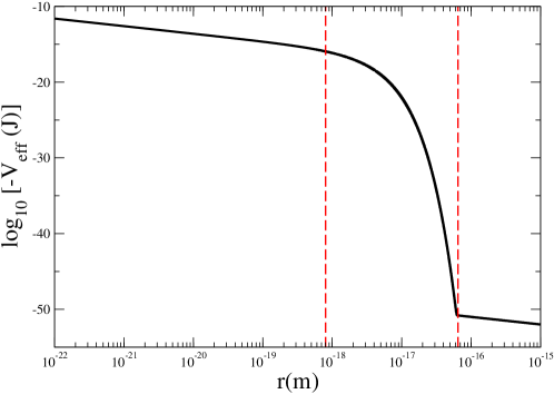
Figure 1: Effective gravitational potential energy between an electron and a hypothetical pointlike proton versus their separation as from Eq. (2). The regions in which the inverse square law hold lie outside the two vertical dashed lines, as evidenced by the identical slopes. In these regions, we expect degeneracy for the 2s-2p contribution within perturbation theory, while in between the dependence on distance removes the degeneracy resulting in a mass-dependent contribution to the Lamb shift. Notice that this intermediate region extends over almost two decades starting at $r_{\mathrm{min}}\simeq\tilde{\Lambda}_{\mathrm{P}}$ and ending at $r_{\mathrm{max}}\simeq 80\tilde{\Lambda}_{\mathrm{P}}$, therefore boosting by almost two orders of magnitude the influence of the lengthscale $\tilde{\Lambda}_{\mathrm{P}}$ at which quantum gravity effects are naturally expected to play a significant role.

A first tool required for our analysis is a proper interpolation between the two regimes of weak gravity at macroscopic distances and the conjectured strong gravity/weak interactions at the microscale. The existence of Newtonian gravitation at large distances, with coupling strength given by the universal gravitational constant $G_{N}$, which can morph into weak interactions corresponding to a renormalized universal gravitational constant $\tilde{G}_{N}$ at small distances, may be obtained by means of a generalized potential energy $V_{\mathrm{eff}}$ for the gravitational interaction between two pointlike particles of mass $m_{1}$ and $m_{2}$

$$V_{\mathrm{eff}}(r)=-\frac{G_{N}m_{1}m_{2}}{r}\left(1+\alpha e^{-r/\lambda}\right)=-\frac{G_{N}m_{1}m_{2}}{r}\left[1+\left(\frac{\tilde{G}_{N}}{G_{N}}-1\right)e^{-r/\tilde{\Lambda}_{\mathrm{P}}}\right],$$ (2)

wherein the intermediate expression we have introduced, as customary in the analysis of Yukawian components of gravity Onofrio1 ; Antoniadis , the generic parameters $\alpha$ and $\lambda$ for the strength and range of the Yukawian component respectively, thereby specialized in the last expression to our case of interest, $\alpha\equiv\tilde{G}_{N}/G_{N}-1$ and $\lambda\equiv\tilde{\Lambda}_{\mathrm{P}}$, with the renormalized Planck length $\tilde{\Lambda}_{\mathrm{P}}=\sqrt{2\hbar\tilde{G}_{N}/c^{3}}=8.014\times 10^{-19}$  m.

Equation 2 reduces to ordinary gravity for $r\gg\tilde{\Lambda}_{\mathrm{P}}$, whereas in the opposite regime of $r\ll\tilde{\Lambda}_{\mathrm{P}}$ continues to have a $1/r$ behaviour but with coupling strength proportional to $\tilde{G}_{N}$. In both limits, the evaluation in perturbation theory of the average gravitational energy should give no difference since $1/r$ potential is degenerate for states with the same principal quantum number and different angular momenta. Therefore, the difference we may evidence in this analysis will reflect the genuine deviation from a inverse square law characteristic of Yukawian potentials. As manifest in Fig. 1 in the concrete example of an electron and a structureless, pointlike proton, the region in which the distance scaling of the corresponding force is not following the inverse square law extends over two decades starting at $r_{\mathrm{min}}\simeq\tilde{\Lambda}_{\mathrm{P}}$.

III Gravitational energy between a lepton and an extended proton: Newtonian component

The evaluation of the gravitational energy between two particles is quantitatively different if one of them has an extended structure, as in the case of the proton. We schematize the proton as a spherical object with uniform mass ensity different from zero only within its electromagnetic radius $R_{p}$ related to the rms charge radius - for a uniform charge density - through $R_{p}=\sqrt{5/3}~{}r_{p}$, in such a way that $\rho_{p}(r)=3m_{p}/(4\pi R_{p}^{3})$ for $r\leq R_{p}$ and zero otherwise. With this assumption, the evaluation of the Newtonian potential energy - the first term in the righthand side of Eq. (2) - between the proton and a generic lepton of mass $m_{\ell}$ ($\ell=e,\mu,\tau$) yields

$$V_{N\ell}(r)=\begin{cases}G_{N}\frac{m_{\ell}m_{p}r^{2}}{2R_{p}^{3}}-\frac{3}{2}G_{N}\frac{m_{\ell}m_{p}}{R_{p}},&\hskip 28.45274pt0<r<R_{p},\\ -G_{N}\frac{m_{\ell}m_{p}}{r},&\hskip 28.45274ptr>R_{p}.\end{cases}$$ (3)

The calculation of the energy contribution due to the Newtonian potential may be performed by means of standard time-independent perturbation theory applied to 2s and 2p states. There is no space anisotropy, so we will focus on the radial (normalized) components of the unperturbed wavefunctions which are, respectively

$$R_{2s}(r)=\frac{1}{(2a_{\ell})^{3/2}}\left(2-\frac{r}{a_{\ell}}\right)e^{-\frac{r}{2a_{\ell}}};\hskip 28.45274ptR_{2p}(r)=\frac{1}{\sqrt{3}(2a_{\ell})^{3/2}}\frac{r}{a_{\ell}}e^{-\frac{r}{2a_{\ell}}},$$ (4)

where $a_{\ell}$ is the Bohr radius, which also takes into account the reduced mass of the lepton-proton bound system. The calculation leads to

$$\langle V_{N\ell}\rangle_{2s} = \langle R_{2s}|V_{N\ell}|R_{2s}\rangle=-\frac{G_{N}m_{\ell}m_{p}}{R_{p}}\times$$

$$\left[-\frac{1}{16\beta^{2}}\left(F_{6}\Big{|}_{0}^{\beta}-4F_{5}\Big{|}_{0}^{\beta}+4F_{4}\Big{|}_{0}^{\beta}\right)+\frac{3}{16}\left(F_{4}\Big{|}_{0}^{\beta}-4F_{3}\Big{|}_{0}^{\beta}+4F_{2}\Big{|}_{0}^{\beta}\right)+\frac{\beta}{8}\left(F_{3}\Big{|}_{\beta}^{+\infty}-4F_{2}\Big{|}_{\beta}^{+\infty}+4F_{1}\Big{|}_{\beta}^{+\infty}\right)\right],$$

$$\langle V_{N\ell}\rangle_{2p} = \langle R_{2p}|V_{N\ell}|R_{2p}\rangle=-\frac{G_{N}m_{\ell}m_{p}}{R_{p}}\left(-\frac{1}{48\beta^{2}}F_{6}\Big{|}_{0}^{\beta}+\frac{1}{16}F_{4}\Big{|}_{0}^{\beta}+\frac{\beta}{24}F_{3}\Big{|}_{\beta}^{+\infty}\right),$$ (6)

where we have introduced $\beta=R_{p}/a_{\ell}$ and $F_{n}\Big{|}_{a}^{b}=\int_{a}^{b}dxx^{n}e^{-x}$.

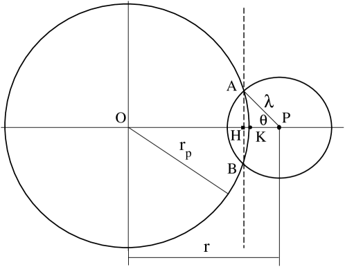
Figure 2: Drawing (not to scale) of the relative proton and lepton coordinates for the evaluation of the Yukawian potential energy term due to the extended structure of the proton. The circle on the left side centered at point O represents the extent of the electric charge distribution of the proton, assumed uniform inside the sphere of radius $R_{p}$. The circle on the right side represents the range of the Yukawian interaction of a pointlike lepton located at point P.

By straightforward algebraic manipulations, we obtain a more compact expression for the Newtonian potential energy difference between the 2s and the 2p state as

$$\Delta\langle V_{N\ell}\rangle_{2s2p}\equiv\langle V_{N\ell}\rangle_{2s}-\langle V_{N\ell}\rangle_{2p}=\frac{G_{N}m_{\ell}m_{p}}{R_{p}}\left[6(e^{\beta}-1)\beta^{-2}-6\beta^{-1}-3-\beta-\frac{\beta^{2}}{4}\right]e^{-\beta},$$ (7)

from which it is easy to see that, in the $\beta\rightarrow 0$ limit of a pointlike proton, $\Delta\langle V_{N\ell}\rangle_{2s2p}\rightarrow G_{N}m_{\ell}m_{p}\beta^{3}e^{-\beta}/(20R_{p})\rightarrow 0$. For a proton of finite size, this contribution is different for hydrogen and muonic hydrogen since the gravitational mass $m_{\ell}$ appears both as a factor and in the expression for the Bohr radius $a_{\ell}$ upon which $\beta$ depends. We notice also that this contribution tends to lift the energy of the 2s state, as this state is more sensitive to the finite size of the proton with respect to the 2p state, analogously to the case of the Coulombian attraction. However, it is also easy to check that the difference is absolutely negligible in our context, being about 37 orders of magnitude smaller than the experimentally observed anomaly in muonic hydrogen, so it cannot play a role in its understanding. This is consistent with a simple estimate of the gravitational contribution in muonic hydrogen based upon consideration of a pointlike proton: from the estimate for the absolute Newtonian potential energy $V_{g}\simeq G_{N}m_{\mu}m_{p}/a_{\mu}\simeq 4.6\times 10^{-34}$ eV, and obviously the presence of an extended structure for the proton, and the differential energy taken in the Lamb shift evaluation, add up to further suppress the Newtonian contribution. This also indicates however that if the Newtonian gravitational constant is boosted by 33 orders of magnitude as in replacing $G_{N}$ with $\tilde{G}_{N}$, the estimate for the absolute energy contribution is in the eV range, making its detailed evaluation relevant to the physics of muonic hydrogen.

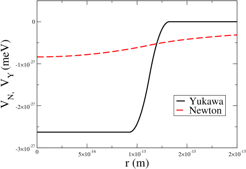
Figure 3: Plot of the Yukawian (continuous black line) and Newtonian (dashed red line) gravitational potential energies in hydrogen corresponding to Eqs. (3) and (10), respectively. The example assumes, to allow for an easier graphical comparison, interaction coupling strength and range as $\tilde{G}_{N}=10^{2}G_{N}$, $\lambda=2.0\times 10^{-16}$ m, and rms charge radius $r_{p}=0.87\times 10^{-15}$ m, while the case considered in this paper has $\tilde{G}_{N}=1.229\times 10^{33}G_{N}$ and $\lambda=\tilde{\Lambda}_{\mathrm{P}}=8.014\times 10^{-19}$ m, leading to a plateau value for the Yukawian component of the potential energy at small distance equal to $\simeq 0.52~{}\mu$eV. The corresponding energy scale for muonic hydrogen is obtained by scaling up the vertical axis by the mass ratio of the two systems, leading to a plateau value $\simeq 0.108$ meV.

IV Gravitational energy between a lepton and an extended proton: Yukawian component

The previous calculation sets the stage for the analysis of the Yukawian component, that is, the second term in the righthand side of Eq. (2). In a semiclassical picture, we expect that if the lepton is outside the proton by at least an amount $\simeq\lambda$, there will be a negligible Yukawian gravitational contribution. Likewise, once the lepton is completely inside the proton, there will be no Yukawian contribution either, as the uniform distribution of the proton mass will extert isotropic interactions. A nonzero value for the proton-lepton interaction occurs instead while the muon is partially penetrating inside the proton radius within a layer of order $\lambda$. The exact calculation for the Yukawian potential felt by the lepton should proceed by integrating the Yukawian potential contributions due to each infinitesimal volume element inside the proton. Since this calculation involves exponential integral functions and it cannot be trivially performed analytically, we introduce two approximations. First, we truncate the Yukawian potential between two pointlike masses at distance $r$ in such a way that

$$V_{Y\ell}(r)=\begin{cases}-\alpha{G}_{N}\frac{m_{\ell}m_{p}}{r},&\hskip 14.22636pt0<r<\lambda,\\ 0,&\hskip 14.22636ptr>\lambda.\end{cases}$$ (8)

Therefore, the evaluation of the potential is carried out only in the region of intersection between two spheres, one of radius equal to $R_{p}$, the other of radius equal to the Yukawa range $\lambda$. In using this approximation, the amplitude of the Yukawian potential is then overestimated in the $0<r<\lambda$ region, while it is underestimated in the region corresponding to $r>\lambda$, as we will discuss more quantitatively at the end of the next section. Second, we further assume that the intersection region is a spherical cap, an approximation corresponding to consider $R_{p}\gg\lambda$, which we will find a posteriori well satisfied.

The potential felt by the lepton at a distance $r$ from the proton center is then evaluated by integrating the infinitesimal potential energy contributions over the volume of the spherical cap of the sphere of radius $\lambda$ centered on the lepton location. With reference to Fig. 2, and using spherical coordinates for the infinitesimal volume $dv$, this can be written as

$$V_{Y\ell}(r)=-\alpha G_{N}m_{\ell}\rho_{p}\int\frac{dv}{\xi}=-\alpha G_{N}m_{\ell}\rho_{p}\int_{0}^{2\pi}d\phi\int_{0}^{\bar{\theta}}dcos\theta\int_{(r-R_{p})/cos\theta}^{\lambda}\xi d\xi,$$ (9)

where $\cos\bar{\theta}=(r-R_{p})/\lambda$. This leads to a Yukawian potential energy as follows

$$V_{Y\ell}(r)=\begin{cases}-2\pi\alpha G_{N}m_{\ell}\rho_{p}\lambda^{2},&\hskip 28.45274pt0<r<R_{p}-\lambda,\\ \pi\alpha G_{N}m_{\ell}\rho_{p}[(r-R_{p})^{2}+2\lambda(r-R_{p})-\lambda^{2}],&\hskip 28.45274ptR_{p}-\lambda<r<R_{p},\\ -\pi\alpha G_{N}m_{\ell}\rho_{p}[(r-R_{p})^{2}-2\lambda(r-R_{p})+\lambda^{2}],&\hskip 28.45274ptR_{p}<r<R_{p}+\lambda,\\ 0,&\hskip 28.45274ptr>R_{p}+\lambda,\end{cases}$$ (10)

in which continuity is ensured at all three boundary regions. As discussed above, this potential corresponds to a net attractive force only in the range $R_{p}-\lambda<r<R_{p}+\lambda$, and zero otherwise, and the plot of the corresponding potential energy is shown in Fig. 3.

We evaluate the expectation value of the Yukawian potential energy in the 2s and 2p states, $\langle V_{Y\ell}\rangle_{2s}$ and $\langle V_{Y\ell}\rangle_{2p}$ according to first-order perturbation theory. The Yukawian component of the gravitational potential is still much smaller that the Coulombian potential even if it is coupled through $\tilde{G}_{\mathrm{N}}$ at short distances, since $\tilde{G}_{\mathrm{N}}m_{\ell}m_{p}<<e^{2}/(4\pi\epsilon_{0})$. The calculation leads to

$$\begin{split}\langle V_{Y\ell}\rangle_{2s}&=-\frac{\pi\alpha G_{N}m_{\ell}\rho_{p}}{4}\Big{[}\lambda^{2}\left(F_{4}\Big{|}_{0}^{y}-4F_{3}\Big{|}_{0}^{y}+4F_{2}\Big{|}_{0}^{y}\right)-\frac{a_{\ell}^{2}}{2}\left(F_{6}\Big{|}_{y}^{\beta}-2(2+v-\beta)F_{5}\Big{|}_{y}^{\beta}-\right.\\ &\left.(4-8v-8\beta+\beta^{2}-2\beta v-v^{2})F_{4}\Big{|}_{y}^{\beta}-4(2v-2\beta+\beta^{2}-2\beta v-v^{2})F_{3}\Big{|}_{y}^{\beta}+4(\beta^{2}-2\beta v-v^{2})F_{2}\Big{|}_{y}^{\beta}\right)+\\ &+\frac{a_{\ell}^{2}}{2}\left(F_{6}\Big{|}_{\beta}^{z}-2(2+v+\beta)F_{5}\Big{|}_{\beta}^{z}+(4+8v+8\beta+\beta^{2}+2\beta v+v^{2})F_{4}\Big{|}_{\beta}^{z}-4(2v+2\beta+\beta^{2}+2\beta v+v^{2})F_{3}\Big{|}_{\beta}^{z}+\right.\\ &\left.+4(\beta^{2}+2\beta v+v^{2})F_{2}\Big{|}_{\beta}^{z}\right)\Big{]},\end{split}$$ (11)

$$\begin{split}\langle V_{Y\ell}\rangle_{2p}&=-\frac{\pi\alpha G_{N}m_{\ell}\rho_{p}}{12}\Big{[}\lambda^{2}F_{4}\Big{|}_{0}^{y}-\frac{a_{\ell}^{2}}{2}\left(F_{6}\Big{|}_{y}^{\beta}+2(v-\beta)F_{5}\Big{|}_{y}^{\beta}+(\beta^{2}-2\beta v-v^{2})F_{4}\Big{|}_{y}^{\beta}\right)+\\ &+\frac{a_{\ell}^{2}}{2}\left(F_{6}\Big{|}_{\beta}^{z}-2(v+\beta)F_{5}\Big{|}_{\beta}^{z}+(\beta^{2}+2\beta v+v^{2})F_{4}\Big{|}_{\beta}^{z}\right)\Big{]},\end{split}$$ (12)

where $y=(R_{p}-\lambda)/a_{\ell}$, $z=(R_{p}+\lambda)/a_{\ell}$, and $v=\lambda/a_{\ell}$.

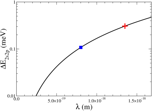
Figure 4: Dependence of the calculated gravitational energy difference between the 2s and 2p energy levels of muonic hydrogen $\Delta E_{2s2p}$ versus the Yukawa range of short-distance gravity. We assume the effective coupling strength as $\tilde{G}_{N}=1.229\times 10^{33}G_{N}=8.205\times 10^{22}~{}\mathrm{m^{3}~{}kg^{-1}~{}s^{-2}}$ which gives rise to the Fermi coupling constant for charged weak interactions as discussed in Onofrio . The CODATA 2010 value of the proton rms charge radius is assumed for the gravitational proton radius. The experimental value for $\Delta E_{2s2p}^{\mathrm{exp}}=$ 0.31 meV is also shown (red cross), which is explained assuming a value of $\lambda=1.35\times 10^{-18}$ m at the effective coupling strength and proton radius assumed above. The prediction of the model for $\lambda=\tilde{\Lambda}_{\mathrm{P}}$, corresponding to $\Delta E_{2s2p}$=0.106 meV, is marked by the blue square.

The difference between the two contributions finally yields, after lengthy algebraic simplifications, the expression

$$\Delta\langle V_{Y\ell}\rangle_{2s2p}\equiv\langle V_{Y}\rangle_{2s}-\langle V_{Y}\rangle_{2p}=-\frac{\alpha G_{N}m_{\ell}m_{p}}{16R_{p}^{3}}\left\{\lambda^{2}f(y)+a_{\ell}^{2}\left[g(y,\beta)+h(\beta,z)\right]\right\},$$ (13)

where $f(y)=2(2-y)y^{3}e^{-y}$ and

$$\begin{split}g(y,\beta)&=-G_{6}\Big{|}_{y}^{\beta}-2(v-\beta)G_{5}\Big{|}_{y}^{\beta}+2\left(-3+v-\beta+\frac{v^{2}}{2}+\beta v-\frac{\beta^{2}}{2}\right)G_{4}\Big{|}_{y}^{\beta}+2(-12-2v+2\beta-v^{2}-2\beta v+\beta^{2})G_{3}\Big{|}_{y}^{\beta}+\\ &12(-1-v+\beta)G_{2}\Big{|}_{y}^{\beta}-24(6+v-\beta)\left(G_{1}\Big{|}_{y}^{\beta}+G_{0}\Big{|}_{y}^{\beta}\right),\end{split}$$

$$\begin{split}h(\beta,z)&=+G_{6}\Big{|}_{\beta}^{z}-2(v+\beta)G_{5}\Big{|}_{\beta}^{z}+2\left(3+v+\beta+\frac{v^{2}}{2}+\beta v+\frac{\beta^{2}}{2}\right)G_{4}\Big{|}_{\beta}^{z}-2(-12+2v+2\beta+v^{2}+2\beta v+\beta^{2})G_{3}\Big{|}_{\beta}^{z}+\\ &12(1-v-\beta)G_{2}\Big{|}_{\beta}^{z}+24(6-v-\beta)\left(G_{1}\Big{|}_{\beta}^{z}+G_{0}\Big{|}_{\beta}^{z}\right),\\ \end{split}$$

where $G_{n}\Big{|}_{a}^{b}=a^{n}e^{-a}-b^{n}e^{-b}$. The sign of the correction is negative, i.e. $\Delta E_{2s2p}<0$, indicating that the 2s state gets more bounded than the 2p state. This outcome is opposite to the case of the long-range Newtonian component in which the 2s state gets a weaker binding since it explores more the proton interior where the net effect of gravity is smaller. This is due to the fact that the Yukawian potential does not fulfil the Gauss theorem and is marginally felt by the 2p state having small overlap with the proton region, unlike in the 2s state. We will indicate from now on the absolute value of $\Delta E_{2s2p}$, with the implicit understanding that it is negative.

The result of this analysis is shown in Figs. 4 and 5, which summarize the main findings of this paper. In Fig. 4, we show $\Delta E_{2s2p}$ as a function of the Yukawa range $\lambda$ for a fixed value of $\alpha$ corresponding to $\tilde{G}_{N}$ as assumed in the text immediately after Eq. (1). For a value of $\lambda=\tilde{\Lambda}_{\mathrm{P}}$, we obtain a value of $\Delta E_{2s2p}\simeq$ 0.106 meV, about a factor 2.8 smaller than the measured value. The experimental value of $\Delta E_{2s2p}$ is instead obtained from Eq. (13) by assuming a value of $\lambda=1.35\times 10^{-18}{\mathrm{m}}\simeq 1.7\tilde{\Lambda}_{\mathrm{P}}$. In spite of the drastic assumption of uniform mass density for the proton inside its electric radius and of the two approximations used in the calculation, the proximity of the prediction on $\Delta E_{2s2p}$ assuming first-principle parameters $\alpha=\tilde{G}_{N}/G_{N}-1$ and $\lambda=\tilde{\Lambda}_{\mathrm{P}}$ as inspired by the conjecture in Onofrio , if not accidental, is rather remarkable. Considering the uncertainty in the relevant proton radius, we have complemented the analysis by showing, in Fig. 5, the combined effect of $\lambda$ and $r_{p}$ on the evaluation of $\Delta E_{2s2p}$. We have also evaluated the points in the $(r_{p},\lambda)$ plane which allow to obtain a value of $\Delta E_{2s2p}$ in the $(0.311,0.309)$ meV interval, see monotonically increasing line. The vertical band is the CODATA 2010 range of values for $r_{p}$, and the horizontal line corresponds to the value of $\lambda=\tilde{\Lambda}_{\mathrm{P}}$. To exactly verify our hypothesis we should have obtained a single intersection point, and this is not achieved within a relative accuracy conservatively estimated to be of order 80 $\%$ in $\lambda$ and 40 $\%$ in $r_{p}$.

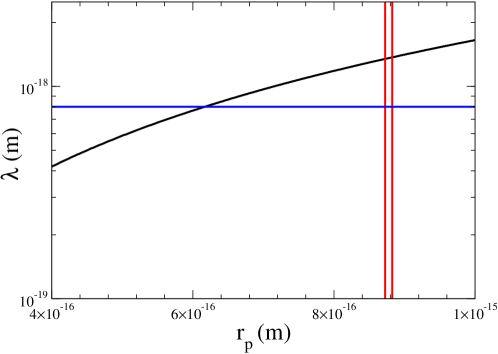
Figure 5: Robustness of the Yukawian gravitational potential with respect to the Yukawa range $\lambda$ and the rms radius $r_{p}$. The locus of the points in the ($\lambda,r_{p}$) plane which give rise to a 0.309 meV $\leq\Delta E_{2s2p}\leq$ 0.311 meV is shown by the monotonically increasing curve. The range of values allowed, within one standard deviation, for the proton rms charge radius according to the CODATA value are delimited by the two vertical lines, the horizontal line corresponding to $\lambda=\tilde{\Lambda}_{\mathrm{P}}$. Complete agreement with the experimental value is obtained for instance by choosing $\lambda\simeq 1.7\tilde{\Lambda}_{\mathrm{P}}$, while having $r_{p}$ at its CODATA value, or by choosing the gravitational radius of the proton equal to $\simeq$ 0.7 times the CODATA value for the rms charge radius while keeping $\lambda=\tilde{\Lambda}_{\mathrm{P}}$.

We further notice that the second approximation, consisting in considering the intersection region between the proton and the Yukawa sphere as a spherical cap, is well-satisfied since the proton radius is more than three orders of magnitude larger than the relevant Yukawa range. The truncation of the Yukawa potential expressed by Eq. (8) is instead a potential source of discrepancy, which can be removed by a numerical analysis with the full Yukawa potential. While this is certainly a subject for future investigation, it is worth to point out that the truncated potential over distance does, in general, overestimate the integral of the Yukawa potential. This can be seen more quantitatively for pointlike particles by considering the zeroth moment of the potential, its integral over the distance, $W_{Y}(r)=\int_{r}^{+\infty}d\xi\exp(-\xi/\lambda)/\xi$, and evaluating the coefficient $\sigma$ such that the zeroth moment of the truncated potential $W_{T\sigma}(r)=\int_{r}^{\sigma\lambda}d\xi/\xi$ equals $W_{Y}(r)$. Alternatively, one can evaluate a multiplicative coefficient $\gamma$ such that $W_{T\gamma}(r)=\gamma\int_{r}^{\lambda}d\xi/\xi$ equals $W_{Y}(r)$. In Fig. 6 we show the dependence of these two correction parameters on the distance $r$, evaluated in units of the Yukawa range $\lambda$. It is evident that in the region of small $r$ of interest for the evaluation of the integrals leading to the potential between the lepton and the proton as an extended structure both $\sigma$ and $\gamma$ are smaller than one. This means that in substituting the Yukawa potential with its truncated approximation one should either replace $\Lambda_{\mathrm{P}}\rightarrow\sigma\Lambda_{\mathrm{P}}$ or $\Delta E_{2s2p}\rightarrow\gamma\Delta E_{2s2p}$. Both procedures go in the direction of increasing the discrepancy discussed around Fig. 4, requiring a larger value of $\lambda$ or a smaller value of $R_{p}$ to accommodate the experimental value of $\Delta E_{2s2p}$.

All possible refinements of the calculations are limited by the fact that in this approach the mass density distribution is crucial, and we do not have any information on the density distribution for the most important component of the proton at the level of determining its mass, i.e. the gluons. This seems currently the most critical issue preventing a more quantitative comparison of the model with the experimental result. It is plausible that gluons, only sensitive to the attractive color interaction, tend to cluster more than valence quarks which are also sensitive to the electromagnetic interaction acting both attractively (between the quarks up and down) and repulsively (between the two quarks up), thereby decreasing the effective gravitational radius of the proton below its electromagnetic value.

In spite of the limitation arising from the lack of knowledge of the gravitational proton radius, it is worth to proceed with the analysis of other systems in which this putative Yukawian potential may also give rise to observable effects and predictions. In this context, here we limit our attention to muonic deuterium and hydrogen. In particular, on the one hand we are able to make a firm prediction for the Lamb shift excess to be expected in muonic deuterium. On the other hand, the analysis of Lamb shift in hydrogen shows that there are potential troubles for the scenario envisaged here, which can be overcome only by relaxing the demand for an economic approach with minimal assumptions.

Muonic deuterium Carboni ; Martynenko ; Krutov may be another viable test of our hypothesis since we expect a significant difference due to the deuterium mass and radius, apart from complications due to the internal mass distribution of deuterium. The calculation for muonic deuterium proceeds by introducing the deuteron charge radius Sick1 recommended by CODATA 2010 as $r_{d}=(2.1424\pm 0.0021)$ fm, and obviously adjusting the mass as corresponding to the deuteron mass. We obtain, at $\lambda=\tilde{\Lambda}_{\mathrm{P}}$, an expected excess in the Lamb energy of 15.5 $\mu$eV, and of 42.6 $\mu$eV at $\lambda=1.35\times 10^{-18}$ m at which the Lamb shift for muonic hydrogen is fully explained. This corresponds to an anomalous frequency shift in the 10 GHz range, smaller than the one in muonic hydrogen but still observable as well above the statistical (0.7 GHz) and systematic (0.3 GHz) uncertainties quoted in Pohl for muonic hydrogen spectroscopy.

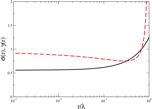
Figure 6: Correction factors $\sigma$ (black, continuous line) and $\gamma$ (red, dashed line) for the truncated potential in Eq. (8) versus the lower integration bound for the zeroth order momentum of the potential energy between two pointlike particles. Both corrections confirm that the overall contribution of the truncated potential is overestimating the Yukawian potential energy.

The predicted anomaly for the Lamb shift in (electronic) hydrogen is instead far too large, corresponding to 0.52 $\mu$eV at $\lambda=\tilde{\Lambda}_{\mathrm{P}}$ and 1.47 $\mu$eV at $\lambda=1.35\times 10^{-18}$ m, if using the same CODATA 2010 proton rms charge radius, and this is potentially a big issue for the validation of the proposed model. The Lamb shift in hydrogen is known with a precision which cannot incorporate such a large contribution, corresponding to an anomalous frequency shift of 0.2 GHz against an absolute accuracy of 9 kHz, or $8.5\times 10^{-6}$ relative accuracy. Among possible ways to circumvent this issue - next to consider the whole model as invalidated - is to assume that the effective interaction corresponding to the Yukawian part in Eq. (2) is flavour-dependent, and does not act among fundamental fermions belonging to the same generation. This is not dissimilar from recent attempts Tucker ; Barger1 ; Batell ; Barger2 to introduce new interactions which differentiates between leptons, and may be also related to the need to understand the role of the electron-muon universality in the theory-experiment discrepancy for the anomalous magnetic moment of the muon Hertzog ; Bennett ; Jegerlehner . A putative “off-diagonal” interaction naturally spoils the universality characteristic of gravitation. However, it should be considered that in a possible gravitoweak unification scheme the emerging structure should presumably incorporate features of both weak and gravitational interactions. The former is manifestly flavor-dependent, as shown in the presence of Cabibbo-Kobayashi-Maskawa (CKM) and Pontecorvo-Maki-Nakagawa-Sakata (PMNS) mixing matrices for the charged current, so it is not a priori impossible that the interaction corresponding to the Yukawa component in Eq. (2) is highly selective in flavour content. This solution could inspire searches for models in which a “hidden sector” of the standard model includes intermediate bosons of mass in the range of the Higgs vacuum expectation value mediating interactions which have mixed features between the usual charged weak interactions and gravitation, for instance heavier relatives of the $Z^{0}$ boson. As a final comment, we would like to also point out that no tests of the equivalence principle have ever been proposed involving other than the first generation of fundamental fermions. It would be interesting in this context to envisage tests of the equivalence principle, for instance free fall experiments involving strange matter such as neutral K mesons.

V Lamb-shift gravitational contribution in purely leptonic systems

We finally complement the analysis by evaluating the contribution of the putative potential in Eq. (2) for purely leptonic systems, such as muonium, a $\mu^{\pm}e^{\mp}$ neutral bound state. Muonium is interesting from the theoretical viewpoint since, due to the pointlike structure of leptons, there are no complications arising from a mass distribution as in the proton case, while experimentally there are complications due to the finite lifetime of the muon. Unfortunately, as we will see below, the expected effect is way too small to be observed, but the related calculations shed also light on the reason for which muonic hydrogen is so effective at spotting a Yukawa contribution with range in the attometer scale. The calculation of the perturbation to the energy levels for muons due to a potential like the one in Eq. (2) leads to the following expressions

$$\langle V_{\mathrm{eff}}\rangle_{2s} = -\frac{G_{N}m_{e}m_{\mu}}{4a_{e\mu}}\left[1+\alpha\left(\frac{2}{(1+\xi)^{2}}-\frac{4}{(1+\xi)^{3}}+\frac{3}{(1+\xi)^{4}}\right)\right],$$ (14)

$$\langle V_{\mathrm{eff}}\rangle_{2p} = -\frac{G_{n}m_{e}m_{\mu}}{4a_{e\mu}}\left[1+\frac{\alpha}{(1+\xi)^{4}}\right],$$ (15)

where $\xi=a_{e\mu}/\lambda$. The contribution to the Lamb shift is then

$$\Delta\langle V_{\mathrm{eff}}\rangle_{2s2p}\equiv\langle V_{\mathrm{eff}}\rangle_{2s}-\langle V_{\mathrm{eff}}\rangle_{2p}=-\alpha\frac{G_{N}m_{e}m_{\mu}}{4a_{e\mu}}\left[\frac{2}{(1+\xi)^{2}}-\frac{4}{(1+\xi)^{3}}+\frac{2}{(1+\xi)^{4}}\right],$$ (16)

in which the Newtonian $1/r$ contribution is obviously canceled out since it is equal in the 2s and 2p states. In the limit of $a_{e\mu}\gg\lambda$ of interest in our considerations, i.e. $\xi\gg 1$, the leading order term is the first in the right-hand side so we get a simplified, yet accurate expression as

$$\Delta\langle V_{\mathrm{eff}}\rangle_{2s2p}\simeq-\frac{\alpha G_{N}m_{e}m_{\mu}\lambda^{2}}{2a_{e\mu}^{3}}.$$ (17)

We obtain $\Delta\langle V_{\mathrm{eff}}\rangle_{2s2p}\simeq 1.85\times 10^{-22}$ eV, corresponding to a frequency shift of $4.48\times 10^{-8}$ Hz. The precision in the determination of the Lamb shift in muonium, of order 1.5 $\%$ Oram ; Badertscher ; Woodle , is not enough to observe the predicted effect in any foreseeable future. A precision observable in muonium is provided by the 1s2s transition frequency. The contribution to the 1s state due to the effective gravitational potential is

$$\langle V_{\mathrm{eff}}\rangle_{1s}=-\frac{G_{N}m_{e}m_{\mu}}{a_{e\mu}}\left[1+\frac{\alpha}{(1+\xi/2)^{4}}\right].$$ (18)

The contribution to the 1s2s frequency then is

$$\Delta\langle V_{\mathrm{eff}}\rangle_{1s2s}\simeq-\frac{7\alpha G_{N}m_{e}m_{\mu}\lambda^{2}}{2a_{e\mu}^{3}},$$ (19)

which leads to a value of the same order of magnitude (just differing by a factor 7) of the 2s2p contribution evaluated above in Eq. (17). Although the 1s2s transition frequency is experimentally determined with a precision of 9.8 MHz Meyer , the expected signal is still too low to provide an observable frequency shift. The situation in principle is less pessimistic for a $\mu^{+}\mu^{-}$ state (the so-called “true muonium”), as the Lamb shift and the 1s2s contributions get increased by a factor $(m_{\mu}/m_{e})^{4}/8$, leading to $\simeq$ 10 Hz for the 2s2p frequency shift, but the very experimental feasibility of muonium is still under debate Brodsky , due to the complications of producing a bound state of two, rather than one, unstable particles.

Nevertheless, this exercise shows the efficacy of muonic hydrogen with respect to purely leptonic, structureless, systems, in which the Bohr radius and the Yukawa range are the only relevant lengthscales. The presence of an intermediate lengthscale, the proton radius, gives a boost in the expected contribution of muonic hydrogen with respect to its muonium counterpart by an amount equal to $(a_{\mu}/R_{p})^{3}\simeq 8\times 10^{6}$, as arguable by means of simple dimensional considerations. In other words, while leptonic systems get a contribution which is quite far from experimental observation, semileptonic systems such as muonic hydrogen instead get an amplified contribution due to the extended structure of the proton which shifts down the relevant lengthscale from $a_{\ell}$ to $R_{p}$, although at the price of introducing a parameter, the proton radius, which is not yet known from first principles. This presumably shows the existence of a narrow window for observing effects due to quantum gravity at the attometer (Fermi) scale. In any event, the fact that muonic hydrogen discriminates between 2s and 2p states, with respect to a Yukawian component of strength much larger than Newtonian gravity and acting on the attometer scale, should make it the first effective “quantum gravimeter”.

VI Conclusions

In conclusion, we have shown that a solution to the “proton radius puzzle” is potentially available by means of an effective Yukawian potential originated by the morphing of Newtonian gravitation into weak interactions at the Fermi scale as conjectured in Onofrio , without additional parameters with respect to the ones already present in the standard model. Leaving aside the need for removing the approximations used in the evaluation of the Yukawa potential due to the proton as an extended object, either the relevant Yukawa range is not coinciding with the Planck scale, or the relevant proton radius is not the one determined using electric probes, or a combination of both factors. Among all these considerations, it is important to point out that the electric charge distribution of the proton investigated by using leptonic probes is not accurately representative of the mass distribution. Within the standard model gluons - which account for a large fraction of the proton mass - do not have electroweak interactions and therefore charged lepton or neutrino scattering off protons cannot provide any information on their spatial distribution. Furthermore, we have been forced to assume that the electron does not interact with the proton via the same effective Yukawian interaction as the muon, since the expected anomalous contribution in the former case is exceedingly large with respect to what is observed in the hydrogen Lamb shift. Although this spoils the requirement for simplicity and universality, it is plausible in light of the complex structure of weak interactions which are flavour- and generation-dependent.

Lastly, it may be worth to briefly discuss possible consequences of our model for future experimental investigations. A very important proposal, as the one described in Gilman on muon-proton scattering, will not add insights on this issue, yet it will be critical in corroborating the existence of the anomaly and to pinpoint any possible deviation from the electron-muon universality. Unfortunately, the intrinsically short lifetime of the $\tau$-lepton of 291 fs makes it unfeasible to perform spectroscopic measurements on tauonic hydrogen, for which the predicted gravitational anomalous Lamb shift is even larger than that for muonic hydrogen. Also, provided that strong interaction effects can be effectively filtered out at the required accuracy level, a systematic study of precision spectroscopy of other exotic atoms with Bohr radii below the picometer range (see Nesvi for a pioneering analysis), such as protonium Venturelli ; Lodi , may allow to confirm or disproof our model in a reasonable time-frame.

- (1) S. G. Karshenboim and V. B. Smirnov (Eds.), Precision Physics of Simple Atomic Systems (Springer-Verlag, 2003).
- (2) I. Sick, Phys. Lett. B 576, 62 (2003).
- (3) P. G. Blunden and I. Sick, Phys. Rev. C 72, 057601 (2005).
- (4) E. Borie and G. A. Rinker, Rev. Mod. Phys. 54, 67 (1982).
- (5) R. Pohl, et al., Nature 466, 213 (2010).
- (6) R. Pohl, R. Gilman, G. A. Miller, and K. Pachucki, Annu. Rev. Nucl. Part. Sci. 63, 175 (2013).
- (7) A. Antognini, et al., Ann. Phys. (N.Y.) 331, 127 (2013).
- (8) A. Antognini, et al., Science 339, 417 (2013).
- (9) V. Barger, et al, Phys. Rev. Lett. 108, 081802 (2012).
- (10) D. Tucker-Smith and Y. Itay, Phys. Rev. D 83, 101702(R) (2011).
- (11) F. Luo and H. Liu, Chin. Phys. Lett. 23, 2903 (2006).
- (12) F. Luo and H. Liu, Int. J. Theor. Phys. 46, 606 (2007).
- (13) Y. X. Liu, X. H. Zhang, and Y. S. Duan, Mod. Phys. Lett. A 23, 1853 (2008).
- (14) Z.-G. Li, W.-T. Ni, and A. P. Patón, Chin. Phys. B 17, 70 (2008).
- (15) L.-B. Wang L-B and W.-T. Ni, Mod. Phys. Lett. A 28, 1350094 (2013).
- (16) J. Ellis, N. E. Mavromatos, and D. V. Nanopoulos, Phys. Lett. B 293, 37 (1992).
- (17) G. Amelino-Camelia , J. Ellis, N. E. Mavromatos, D. V. Nanopoulos, and S. Sarkar, Nature 393, 763 (1998).
- (18) G. Amelino-Camelia, Mod. Phys. Lett. A 17, 899 (2002).
- (19) G. Amelino-Camelia, Quantum Gravity Phenomenology, in D. Orti (Ed.), Approaches to Quantum Gravity: Toward a new understanding of space, time and matter, Cambridge University Press, UK, 2009, p. 427.
- (20) R. Onofrio, Mod. Phys. Lett. A 28, 1350022 (2013).
- (21) F. W. Hehl, P. von der Heyde, G. Kerlick, and J. M. Nester, Rev. Mod. Phys. 48, 393 (1976).
- (22) F. W. Hehl and B. K. Datta, J. Math. Phys. 12, 1334 (1971).
- (23) N. A. Batakis, Phys. Lett. B 148, 51 (1984).
- (24) N. A. Batakis, Class. Quant. Grav. 3, L99 (1986).
- (25) Yu. M. Loskutov, J. Exp. Theor. Phys. 80, 150 (1995).
- (26) S. Capozziello, M. De Laurentis, L. Fabbri, and S. Vignolo, Eur. Phys. J. C 72, 1908 (2012).
- (27) X. Calmet, S. D. H. Hsu, and D. Reeb, Phys. Rev. D 77, 125015 (2008).
- (28) R. Onofrio, New J. Phys. 8, 237 (2006).
- (29) I. Antoniadis, S. Baessler, M. Büchner, V. V. Fedorov, S. Hoedl, A. Lambrecht, V. V. Nesvizhevsky, G. Pignol, K. V. Protasov, S. Reynaud, and Yu. Sobolev, C. R. Physique 12, 755 (2011).
- (30) G. Carboni, Lett. Nuovo Cimento 7, 160 (1973).
- (31) A. P. Martynenko, J. Exp. Theor. Phys. 101, 1021 (2005).
- (32) A. A. Krutov and A. P. Martynenko, Phys. Rev. A 84, 052514 (2011).
- (33) I. Sick and D. Trautmann, Nucl. Phys. A 637, 559 (1998).
- (34) V. Barger, C.-W. Chiang, W.-Y. Keung, and D. Marfatia, Phys. Rev. Lett. 106, 153001 (2011).
- (35) B. Batell, D. McKeen, and M. Pospelov, Phys. Rev. Lett. 107, 011803 (2011).
- (36) V. Barger, C.-W. Chiang, W.-Y. Keung, and D. Marfatia, Phys. Rev. Lett. 108, 081802 (2012).
- (37) D. W. Hertzog and W. M. Morse, Ann. Rev. Nucl. Part. Phys. Sci. 54, 141 (2004).
- (38) G. Bennett et al., Phys. Rev. D 73, 072003 (2006).
- (39) F. Jegerlehner and A. Nyffeler, Phys. Rep. 477, 1 (2009).
- (40) C. J. Oram, et al., Phys. Rev. Lett. 52, 910 (1984).
- (41) A. Badertscher, et al., Phys. Rev. Lett. 52, 914 (1984).
- (42) K. A. Woodle, et al., Phys. Rev. A 41, 93 (1990).
- (43) V. Meyer et al., Phys. Rev. Lett. 84, 1136 (2000).
- (44) S. J. Brodsky and R. F. Lebed, Phys. Rev. Lett. 102, 213401 (2009).
- (45) R. Gliman, et al., arXiv:1303.2160.
- (46) V. V. Nesvizhevsky and K. V. Protasov, Class. Quantum Grav. 21, 4557 (2004).
- (47) L. Venturelli, et al., Nucl. Instr. Meth. Phys. B 261, 40 (2007).
- (48) E. Lodi Rizzini, et al., Eur. Phys. J. Plus 127, 124 (2012).