The range and nature of effective interactions in hard-sphere solids
	Michael Schindler∗a and A. C. Maggsa
	Colloidal systems observed in video microscopy are often analysed using the displacements correlation matrix of particle positions. In non-thermal systems, the inverse of this matrix can be interpreted as a pair-interaction potential between particles. If the system is thermally agitated, however, only an effective interaction is accessible from the correlation matrix. We show how this effective interaction differs from the non-thermal case by comparing with high-statistics numerical data from hard-sphere crystals.

1 Introduction

The analysis of the displacement–displacement correlation function between many particles has become a standard tool used on experimental data ^{1, 2, 3, 4, 5} acquired by video and confocal microscopy as well as on numerical data.^{6, 7, 8, 9} It is much, but not exclusively, used by researchers interested in jammed and glassy dynamics of soft particles. In practice, one first determines the reference positions of particles and then records the correlations of displacements with respect to these reference positions for all particles. The averages are done either over time, using particle trajectories, or over an ensemble, using Monte-Carlo sampling. The result is a large correlation matrix $G$ between all displacements of all particles, which is then inverted to give another matrix $D$.

This matrix $D$ is often interpreted as an effective interaction matrix which characterises oscillations of the particles around their reference positions. In that context, $D$ is called the dynamical matrix.^{10, 7} This interpretation has its origins in the analysis of non-thermal systems where massive particles are connected by harmonic or other interaction potentials. The dynamical matrix is then proportional to the Hessian matrix $H$ of second derivatives of the total interaction potential⁷ (with the particle mass and with $kT$ as proportionality factors, which will play no role in the following). When activated by a small external stimulus, the response of the system is a mixture of oscillations which are given by the eigenfrequencies and eigenvectors of the dynamical matrix. One condition for this analysis to remain true is that the oscillation amplitudes are small, so that the dynamical matrix does not depend on the displacements. With the masses of the particles and the measured correlation matrix $G$ as input, one can obtain information about the interaction potential between the particles.

The protocol to record data and to invert the matrix $G$ works equally well on thermal as on non-thermal systems. In contrast to the Hessian matrix $H$, which contains the static potential interactions, the matrix $G^{-1}$ contains also all the thermal contributions, including entropic. How is the dynamical matrix changed by these contributions? To what extent can we still infer the interaction between particles? For example, if the true interaction acts only between nearest neighbours, the same is true for $H$, but does it also hold for the effective interactions obtained from $G^{-1}$?

Between these two limits of completely non-thermal $H$ and fully thermal $G^{-1}$, a plethora of intermediate levels can be identified, which account for more or fewer aspects of the thermal distribution and which may serve for more or less reasonable models for the observed system. We refer to Henkes et al. ⁷ for a review of some of these intermediate levels and the connections between them, such as the harmonic approximation or the shadow system. As we mention models for the system, it is important to note that the Hessian matrix with which we compare $G^{-1}$ may derive from modelling potentials very different from the true ones.

The aim of the present paper is to establish the difference between the two extreme cases, which are the non-thermal case (Hessian matrix $H$) and the fully thermal matrix $G^{-1}$ obtained from observation data. We here want to see the largest difference and therefore choose as system of observation a crystal of hard spheres which collide elastically. It is usually said that thermal (entropic) effects are maximal in the hard-sphere system. We also have to choose a model system of which we calculate the Hessian matrix. We here take the most general form of pairwise, central potential interactions.

Beside its interpretation as effective interactions, the matrix $G^{-1}$ – and more directly the correlation matrix $G$ – serve also to extract elastic moduli from thermal fluctuations. Because the elastic moduli are macroscopic quantities of the whole system, this measurement involves only large-wavelength properties of the effective interactions contained in $G^{-1}$. Of course, the same procedure can be done in the non-thermal case using $H$ instead of $G^{-1}$. One advantage of the elastic moduli is that their calculation is not limited to smooth pairwise potentials but applies to other types of interaction as well, such as strictly hard spheres. We expect to see here another discrepancy between the thermal and the non-thermal cases: When one searches the long-wavelength limit of the Hessian matrix, one obtains the so-called Cauchy relations which reduce the number of independent elastic constants in materials below the number expected from symmetry considerations. For example, in two-dimensional hexagonal crystals and in three-dimensional cubic crystals the Cauchy relations can be written as an equality $\lambda=\mu$ between two Lam coefficients. The Cauchy relations apply if interactions between atoms (or colloids) are pairwise, central, sufficiently short ranged, and if thermal fluctuations are neglected. The role of thermal fluctuations was clarified by Squire et al. ¹¹ who calculated the extra contributions (beyond those found by Born and Huang ¹⁰) in the expressions for the elastic constants at nonzero temperature. These contributions can be seen as the “entropic” part of the elastic moduli, and they explain why hard-sphere crystals do not satisfy the Cauchy relations ¹².

The paper is structured as follows: In section 2 we collect some results from known theories, in particular from the non-thermal dynamical (Hessian) matrix. We derive some properties of the dynamical matrix which allow comparison with the fully thermal case. The numerical data for the hard-sphere crystals is then presented in section 3 in one, two and three dimensions. Finally, in section 4 we discuss the observed differences between the two cases.

2 Effective interactions and the central force model

The simplest (Cauchy) model of elasticity in the physics of solids supposes that interactions are pairwise and central between all particles in the solid, deriving from a scalar potential, see for example § 29 of the book by Born and Huang ¹⁰. In this section we study the elastic properties of such systems, in order to better understand where the numerical data demonstrate the presence of non-central potentials.

In this model, the total potential energy $\Phi$ of a configuration is a function of all particle positions $\mathbf{r}_{\mathbf{i}}$. It is expressed as a sum of central pair-potentials $g_{\mathbf{i}\mathbf{j}}$,

$$\Phi(\{\mathbf{r}\})=\sum_{(\mathbf{i}\mathbf{j})}g_{\mathbf{i}\mathbf{j}}\bigl{(}(\mathbf{r}_{\mathbf{i}}-\mathbf{r}_{\mathbf{j}})^{2}/2\bigr{)}$$ (1)

The sum runs over all different pairs of particles. To simplify the algebra and avoid square roots in the calculations, the $g_{\mathbf{i}\mathbf{j}}$ are functions of the distance squared. The functions should be identical for symmetry-related pairs of particles, but otherwise each function is independent.

In order to unify the notation with the numerical simulations of later sections, we assume already here that the particles are in a crystalline configuration (hexagonal or face-centered cubic, depending on the number of spatial dimensions). Throughout the paper, $\mathbf{i},\mathbf{j},\mathbf{m},\mathbf{n}$ denote tuples of integer indices on the Bravais lattice and serve to identify the sites on the lattice. Spatial indices are denoted by Greek letters. The spatial (Euclidean) positions of lattice sites are denoted by vectors $\mathbf{R}_{\mathbf{i}}$. They are multiples of the lattice spacing $d_{0}$. The numerical, and optionally also the theoretical calculations, are periodic in space. All differences between lattice indices, $\mathbf{i}-\mathbf{j}$, or lattice positions, $\mathbf{R}_{\mathbf{i}\mathbf{j}}:=\mathbf{R}_{\mathbf{i}-\mathbf{j}}=\mathbf{R}_{\mathbf{i}}-\mathbf{R}_{\mathbf{j}}$ are thus understood modulo the periodicity, the result being mapped back into a centered copy of the periodic box.

2.1 Description in terms of local displacements

We now calculate the Hessian matrix of the potential energy $\Phi(\{\mathbf{r}\})$ around the crystalline reference state. This amounts to small-amplitude displacements, which are non-thermal in their nature. The reference state has inversion symmetry (hexagonal in 2D, face-centered cubic in 3D), which imposes that the partial first derivatives vanish when evaluated at the reference positions:

$$\frac{\partial\Phi}{\partial r_{\mathbf{i}\alpha}}\bigl{(}\{\mathbf{R}\}\bigr{)}=0$$ (2)

for all $\mathbf{i}$ and $\alpha$. From Eq. (2) it follows that the increase in potential energy of the system due to local displacements is given to quadratic order by

$$\Delta\Phi:=\Phi\bigl{(}\{\mathbf{r}\}\bigr{)}-\Phi\bigl{(}\{\mathbf{R}\}\bigr{)}=\frac{1}{2}\sum_{\alpha,\beta,\mathbf{i},\mathbf{j}}H_{\alpha\beta}(\mathbf{j}-\mathbf{i})\,u_{\mathbf{i}\alpha}\,u_{\mathbf{j}\beta}$$ (3)

where $\mathbf{u}_{\mathbf{i}}=\mathbf{r}_{\mathbf{i}}-\mathbf{R}_{\mathbf{i}}$ is the displacement vector of particle $\mathbf{i}$. The Hessian matrix consists of second derivatives, evaluated at the reference positions,

$$H_{\alpha\beta}(\mathbf{j}-\mathbf{i}):=\frac{\partial^{2}\Phi}{\partial r_{\mathbf{i}\alpha}\partial r_{\mathbf{j}\beta}}\bigl{(}\{\mathbf{R}\}\bigr{)}.$$ (4)

Start with the first derivative

$$\frac{\partial\Phi}{\partial x_{\mathbf{i}}}\bigl{(}\{\mathbf{r}\}\bigr{)}=\sum_{\mathbf{j}\neq\mathbf{i}}(x_{\mathbf{i}}-x_{\mathbf{j}})g^{\prime}_{\mathbf{i}\mathbf{j}}$$ (5)

and obtain $H_{\alpha\beta}(\mathbf{j}-\mathbf{i})$ for $\mathbf{i}\neq\mathbf{j}$:

$$H_{\alpha\beta}(\mathbf{j}-\mathbf{i})=-(R_{\mathbf{i}\alpha}{-}R_{\mathbf{j}\alpha})(R_{\mathbf{i}\beta}{-}R_{\mathbf{j}\beta})\,g^{\prime\prime}_{\mathbf{i}\mathbf{j}}-\delta_{\alpha\beta}\,g^{\prime}_{\mathbf{i}\mathbf{j}},$$ (6)

We abbreviate our notation by introducing $\mathbf{R}_{\mathbf{j}-\mathbf{i}}=\mathbf{R}_{\mathbf{j}}-\mathbf{R}_{\mathbf{i}}$ and $g_{\mathbf{j}-\mathbf{i}}=g_{\mathbf{i}\mathbf{j}}$ and obtain

$$H_{\alpha\beta}(\mathbf{n})=-R_{\mathbf{n}\alpha}R_{\mathbf{n}\beta}\,g^{\prime\prime}_{\mathbf{n}}\bigl{(}R_{\mathbf{n}}^{2}/2\bigr{)}-\delta_{\alpha\beta}\,g^{\prime}_{\mathbf{n}}\bigl{(}R_{\mathbf{n}}^{2}/2\bigr{)}.$$ (7a)

At $$\mathbf{j}=\mathbf{i} \mathbf{n}$$, the matrix is constrained by the fact that the sum over all vanishes,

$$H_{\alpha\beta}(\mathbf{0})=-\sum_{\mathbf{n}\neq\mathbf{0}}H_{\alpha\beta}(\mathbf{n}).$$ (7b)

Let us return for a moment to the meaning of this Hessian matrix. As was mentioned in the introduction, it is also the dynamical matrix of particles (of unit mass), in the sense that their displacements oscillate around the reference state according to the equation

$$\ddot{\mathbf{u}}_{\mathbf{i}\alpha}=-\sum_{\mathbf{j},\beta}H_{\alpha\beta}(\mathbf{j}-\mathbf{i})\mathbf{u}_{\mathbf{j}\beta}.$$ (8)

In words, the interaction matrix $H_{\alpha\beta}(\mathbf{i}-\mathbf{j})$ governs the force exerted on particle $\mathbf{i}$ by particle $\mathbf{j}$. For every separation vector $\mathbf{n}$ between two particles, $H_{\alpha\beta}(\mathbf{n})$ is a $d{\times}d$-matrix. We will find it important to analyse the forces and displacements parallel and orthogonal to the separation vector $\mathbf{n}$. In particular in two dimensions, we can use the rotated orthonormal basis $(\hat{\mathbf{R}}_{\mathbf{n}},\hat{\mathbf{o}})$, where the hat denotes a normalised vector, to define the rotated components of the matrix $H(\mathbf{n})$. We find

$$H_{\parallel}(\mathbf{n}) :=\hat{\mathbf{R}}_{\mathbf{n}}^{T}H(\mathbf{n})\hat{\mathbf{R}}_{\mathbf{n}}=-\mathbf{R}_{\mathbf{n}}^{2}g^{\prime\prime}_{\mathbf{n}}(\mathbf{R}_{\mathbf{n}}^{2}/2)-g^{\prime}_{\mathbf{n}}(\mathbf{R}_{\mathbf{n}}^{2}/2)$$ (9a)

$$H_{\perp}(\mathbf{n}) :=\hat{\mathbf{o}}^{T}H(\mathbf{n})\hat{\mathbf{o}}=-g^{\prime}_{\mathbf{n}}(\mathbf{R}_{\mathbf{n}}^{2}/2)$$ (9b)

$$H_{\text{sym}}(\mathbf{n}) :=\bigl{(}\hat{\mathbf{R}}_{\mathbf{n}}^{T}H(\mathbf{n})\hat{\mathbf{o}}+\hat{\mathbf{o}}^{T}H(\mathbf{n})\hat{\mathbf{R}}_{\mathbf{n}}\bigr{)}/2=0$$ (9c)

$$H_{\text{asym}}(\mathbf{n}) :=\bigl{(}\hat{\mathbf{R}}_{\mathbf{n}}^{T}H(\mathbf{n})\hat{\mathbf{o}}-\hat{\mathbf{o}}^{T}H(\mathbf{n})\hat{\mathbf{R}}_{\mathbf{n}}\bigr{)}/2=0$$ (9d)

The components $H_{\parallel}$ and $H_{\perp}$ control those components of the force which are parallel to the displacements, respectively both parallel to $\mathbf{n}$ ($H_{\parallel}$) or both orthogonal to it ($H_{\perp}$). The (a)symmetric parts govern those components of the force which are orthogonal to the displacements they result from. They are found to vanish in the present model, meaning that displacements can generate only forces which are parallel to them. This property appears as a result of the potentials being central, and it will be tested on the numerical data in the sections below.

We can also examine the results in the non-rotated frame. In particular, for the off-diagonal terms we find

$$H_{xy}(\mathbf{n})=-X_{\mathbf{n}}Y_{\mathbf{n}}g^{\prime}_{\mathbf{n}}\bigl{(}R_{\mathbf{n}}^{2}/2\bigr{)}.$$ (10)

which is an odd function with respect to $X_{\mathbf{n}}$ and to $Y_{\mathbf{n}}$. Also this symmetry will be subject to comparison with the numerical data.

2.2 Long-wavelength limit

The elastic tensor for the model (1) has been calculated by Born and Huang ¹⁰ (§ 29). In our notation, their result for the elastic tensor reads

$${\bar{C}}_{\alpha\sigma\beta\tau}=\frac{N}{2V}\sum_{\mathbf{n}}R_{\mathbf{n},\alpha}R_{\mathbf{n},\sigma}R_{\mathbf{n},\beta}R_{\mathbf{n},\tau}\,g^{\prime\prime}_{\mathbf{n}}\bigl{(}R_{\mathbf{n}}^{2}/2\bigr{)}.$$ (11)

Here, $N$ is the number of particles, and $V$ is the volume of the (periodic) box. We use an overbar to distinguish this tensor from the true (thermal) elastic tensor. Expression (11) is symmetric under all index permutations, which is higher than the symmetry required for the elastic tensor. This observation leads us directly to the Cauchy relation: The general form of the elastic tensor is given by group theory, for example in a two-dimensional hexagonal lattice,

$$C_{\alpha\beta\sigma\tau}=\lambda\delta_{\alpha\beta}\delta_{\sigma\tau}+\mu\bigl{(}\delta_{\alpha\sigma}\delta_{\beta\tau}+\delta_{\alpha\tau}\delta_{\beta\sigma}\bigr{)},$$ (12)

with the Lam coefficients $\lambda$ and $\mu$. This expression becomes completely symmetric under index permutations only if the Cauchy relation $\lambda=\mu$ is satisfied. The situation is similar in three-dimensional cubic lattices, only that there is another term in Eq. (12) with the anisotropy coefficient as prefactor. There, the Cauchy relation reduces three independent coefficients to two. In Section 3 we will measure the Lam coefficients from numerical data and test directly whether the Cauchy relation is satisfied.

When we determine the Lam coefficients from Eq. (11), we find indeed that they are identical,

$${\bar{\lambda}}={\bar{\mu}} =\frac{N}{16V}\sum_{\mathbf{n}}R_{\mathbf{n}}^{4}g^{\prime\prime}_{\mathbf{n}}$$

$$=\frac{N}{16V}\sum_{\mathbf{n}}R_{\mathbf{n}}^{2}\bigl{(}H_{\perp}(\mathbf{n})-H_{\parallel}(\mathbf{n})\bigr{)}.$$ (13)

In the last step we made use of Eqs. (9a) and (9b).

We must mention that the calculation by Born and Huang ¹⁰ is done with a stress-free reference state in mind. In model (1) we do not know a priori whether the stress vanishes in the reference state or not, and for the hard-sphere crystals in the sections below, we know that they stay crystalline only if they are sufficiently compressed by the periodic box. We therefore need to consider the general case of a non-vanishing stress in the reference state. The effect of this stress is that the elastic tensor $C$, which characterises the quadratic increase of free energy with strain, is not identical to the elastic tensor $A$ which characterises the motion of long-wavelength vibrations and thermal excitations.¹³ The two tensors are related by

$$A_{\alpha\beta\sigma\tau}:=C_{\alpha\beta\sigma\tau}+T_{\beta\tau}\delta_{\alpha\sigma},$$ (14)

where $T$ denotes the stress tensor in the reference state. To obtain the stress tensor, we start with the force between two particles,

$$\mathbf{f}_{\mathbf{i}\mathbf{j}}=-(\mathbf{R}_{\mathbf{i}}-\mathbf{R}_{\mathbf{j}})g^{\prime}_{\mathbf{i}\mathbf{j}}.$$ (15)

The virial part of the stress tensor is thus

$${\bar{T}}_{\sigma\tau}=-\frac{1}{2V} \sum_{(\mathbf{i}\mathbf{j})}{(\mathbf{R}_{\mathbf{i}}-\mathbf{R}_{\mathbf{j}})}_{\sigma}f_{\mathbf{i}\mathbf{j},\tau}$$

$$=\frac{N}{2V} \sum_{\mathbf{n}}R_{\mathbf{n},\sigma}R_{\mathbf{n},\tau}g^{\prime}_{\mathbf{n}}.$$ (16)

This expression has been given also by Born and Huang ¹⁰.

It is desirable to derive expression (11) directly from a long-wavelength limit of the interaction matrix $H$. This calculation cannot be done at this point, since we require thermal fluctuations which then yield the tensor $A$. From there we can conclude on the tensor $C$. We therefore defer this calculation to section 3.2.2 below, where we will do it on the matrix $D$. When we replace $D(\mathbf{n})$ by $H(\mathbf{n})/kT$ in the result (30) there, we find the equivalent of the elastic tensor $A$,

$${\bar{A}}_{\alpha\sigma\beta\tau}:=-\frac{N}{2V}\sum_{\mathbf{n}}R_{\mathbf{n},\sigma}R_{\mathbf{n},\tau}H_{\alpha\beta}(\mathbf{n})\\ =\frac{N}{2V}\sum_{\mathbf{n}}R_{\mathbf{n},\sigma}R_{\mathbf{n},\tau}\bigl{(}R_{\mathbf{n},\alpha}R_{\mathbf{n},\beta}\,g^{\prime\prime}_{\mathbf{n}}+\delta_{\alpha\beta}\,g^{\prime}_{\mathbf{n}}\bigr{)},$$ (17)

which is entirely compatible with Eqs. (11), (14) and (16).

2.3 Description in terms of global deformations

In the above section we expressed the elastic constants in terms of a long-wavelength limit of the matrix $H$. This matrix, as it involves second derivatives of the potential energy only, is non-thermal in nature. At least for the elastic constants, it is possible to include thermal effects¹¹. We introduce a parameter for global deformations of the system, the strain $\eta$ and perform a Taylor expansion of the Free Energy $F(\eta)=-kT\ln(Z(\eta))$ about zero strain ($\eta=0$). As the whole box is changed parametrically, we could speak of a “zero-wavevector” ($|\mathbf{Q}|=0$) method instead of the long-wavelength limit $|\mathbf{Q}|\to 0$. The resulting stress tensor and elastic tensor are expressed by the usual Gibbs-weighted average over configurations,¹¹

$$T_{\alpha\beta} =\frac{1}{V}\frac{\partial F}{\partial\eta_{\alpha\beta}}(0)$$

$$=-kT\frac{N}{V}\delta_{\alpha\beta}+\frac{1}{V}\Bigl{\langle}{\textstyle\sum\limits_{(\mathbf{i}\mathbf{j})}}\>g_{\mathbf{i}\mathbf{j}}^{\prime}\bigl{(}r_{\mathbf{i}\mathbf{j}}^{2}/2\bigr{)}\,r_{\mathbf{i}\mathbf{j},\alpha}\,r_{\mathbf{i}\mathbf{j},\beta}\Bigr{\rangle}$$ (18)

$$C_{\alpha\beta\sigma\tau} =\frac{1}{V}\frac{\partial^{2}F}{\partial\eta_{\alpha\beta}\partial\eta_{\sigma\tau}}(0)=2kT\frac{N}{V}\delta_{\alpha\tau}\delta_{\beta\sigma}$$

$$-\frac{1}{V\,kT}\operatorname{Ccc}\Bigl{(}{\textstyle\sum\limits_{(\mathbf{i}\mathbf{j})}}\>g_{\mathbf{i}\mathbf{j}}^{\prime}\bigl{(}r_{\mathbf{i}\mathbf{j}}^{2}/2\bigr{)}\,r_{\mathbf{i}\mathbf{j},\alpha}\,r_{\mathbf{i}\mathbf{j},\beta},\;{\textstyle\sum\limits_{(\mathbf{i}\mathbf{j})}}\>g_{\mathbf{i}\mathbf{j}}^{\prime}\bigl{(}r_{\mathbf{i}\mathbf{j}}^{2}/2\bigr{)}\,r_{\mathbf{i}\mathbf{j},\sigma}\,r_{\mathbf{i}\mathbf{j},\tau}\Bigr{)}$$

$$+\frac{1}{V}\Bigl{\langle}{\textstyle\sum\limits_{(\mathbf{i}\mathbf{j})}}\>g_{\mathbf{i}\mathbf{j}}^{\prime\prime}\bigl{(}r_{\mathbf{i}\mathbf{j}}^{2}/2\bigr{)}\,r_{\mathbf{i}\mathbf{j},\alpha}\,r_{\mathbf{i}\mathbf{j},\beta}\,r_{\mathbf{i}\mathbf{j},\sigma}\,r_{\mathbf{i}\mathbf{j},\tau}\Bigr{\rangle}$$ (19)

The function $\operatorname{Ccc}(a,b):=\langle ab\rangle-\langle a\rangle\langle b\rangle$ is a cumulant-like cross-correlation function. The terms on the right-hand side of Eq. (18) are called the kinetic and the virial terms. The terms in Eq. (19) are called the kinetic term, the fluctuations term, and the Born term.¹¹

The virial term in (18) and the Born term in (19) resemble much the expressions we found for stress (16) and elastic tensor (11) from model (1). Only, there we evaluated at the reference positions, and here we average over positions around these reference positions. Of course, if the position distribution is very narrow, the values obtained from both can be close. Both kinetic terms and the fluctuation term are missing, however. The absence of these terms is where the tensor ${\bar{C}}$ has its higher symmetry from, and why we obtained the Cauchy relation for it.

The elastic tensor (19) includes all thermal effects, because we take the second derivative of the free energy. A similar derivative of the potential energy (1) would simply yield again the Born-like term in (11). It would be very nice to add thermal effects to the interaction matrix, just by replacing the potential energy by the free energy in the second derivative with respect to the reference positions $\mathbf{R}_{\mathbf{i}}$. Unfortunately, the reference positions are not parameters, they appear by a spontaneous symmetry breaking, and we therefore do not know how to do such a derivative. For the moment, we can only work with the imperfect expressions of the above sections and compare them with full numerical data.

3 Numerical results from Hard sphere simulations

We performed high statistics event-driven molecular dynamics simulations of $N$ hard spheres in one, two and three dimensions ($d=1,2,3$). In one dimension the particles were confined to a line. In two dimensions we simulated a hexagonal crystal within a box adapted to the Bravais lattice. In three dimensions we performed simulations of face-centred cubic crystals, again within a box adapted to the Bravais lattice. In all dimensions the simulation box was continued periodically. During a simulation the total momentum and the (kinetic) energy were conserved. The densities were always so high that no particle interchange occurred over the simulation time, so that particle diffusion and defects can be neglected in the data analysis. The Bravais lattice thus defines the reference positions of the spheres, and these coincide with the average positions.

For all numerical data the units are chosen such that the particles have unit diameter, unit mass, and that $kT=1$ with $T$ the temperature.

During the simulation we took a series of $K$ data recordings. For each recording, we measure the deviations $\mathbf{u}_{\mathbf{i}}:=\mathbf{r}_{\mathbf{i}}-\mathbf{R}_{\mathbf{i}}$ of the instantaneous particle positions from their reference positions and calculate the $dN{\times}dN$ correlation matrix

$$G_{(\mathbf{i},\alpha)(\mathbf{j},\beta)}:=\frac{1}{K}\sum_{k=1}^{K}u_{\mathbf{i}\alpha}u_{\mathbf{j}\beta}$$ (20)

The matrix has a simple physical interpretation from linear response theory: It determines the vectorial displacement at $\mathbf{j}$ due to a force at $\mathbf{i}$. We will thus call it a Green function in the following. In order to reduce statistical noise, we average elements of $G$ which are related by the translational symmetry of the lattice,

$$G_{\alpha\beta}(\mathbf{n}):=\frac{1}{N}\sum_{\mathbf{i}}G_{(\mathbf{i},\alpha)(\mathbf{i}+\mathbf{n},\beta)}.$$ (21)

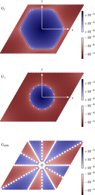
Fig.  1: The two-dimensional Green function in a periodic $32{\times}32$ hexagonal lattice. Plotted are the components of the $2{\times}2$ matrices $G_{\alpha\beta}(\mathbf{n})$ in a rotated orthonormal basis $(\hat{\mathbf{R}}_{\mathbf{n}},\hat{\mathbf{o}})$: $G_{\parallel}=\hat{\mathbf{R}}_{\mathbf{n}}^{T}G\hat{\mathbf{R}}_{\mathbf{n}}$, $G_{\perp}=\hat{\mathbf{o}}^{T}G\hat{\mathbf{o}}$, $G_{\text{sym}}=(\hat{\mathbf{R}}_{\mathbf{n}}^{T}G\hat{\mathbf{o}}+\hat{\mathbf{o}}^{T}G\hat{\mathbf{R}}_{\mathbf{n}})/2$. The antisymmetric off-diagonal terms vanish to within statistical noise ($\pm 10^{-9}$). In the lowest panel the white lines correspond to a mechanical response parallel to an imposed force.

The sum runs over all sites of the Bravais lattice. We could also average over the rotational and inversion symmetries, but we prefer to see the symmetries appear from the data in order get a idea of the statistical errors; the translational average appears to be sufficient for noise reduction. A visual representation of the elements of $G(\mathbf{n})$ in two dimensions is given in Fig. 1. It is a rather structureless object, and it depends on the size and shape of the periodic box due to the logarithmic nature of two-dimensional Green functions. In the figure we plot the elements of $G(\mathbf{n})$ in a rotated coordinate system with one basis vector aligned with the vector $\mathbf{R}_{\mathbf{n}}$. We note in particular the interesting physical structure that occurs in the off-diagonal elements. These elements of the response function vanish along high symmetry directions: a force along these symmetry directions gives a purely parallel displacement. This gives rise to a set of radial white lines in the lowest panel of Fig. 1.

We then use matrix algebra to numerically invert the large matrix $G$ to produce the effective interaction matrix $D$. More precisely, we use the translation-averaged $dN{\times}dN$ matrix

$$G_{\alpha\beta}(\mathbf{i},\mathbf{j}):=G_{\alpha\beta}(\mathbf{j}-\mathbf{i}).$$ (22)

and take its Moore–Penrose pseudoinverse because we must avoid inversion of the zero eigenvalues in $G$ which come from momentum conservation. The inverse is denoted by $D_{\alpha\beta}(\mathbf{i},\mathbf{j})$. In the following, we will analyse the properties of the resulting $2{\times}2$ matrices

$$D_{\alpha\beta}(\mathbf{n}):=\frac{1}{N}\sum_{\mathbf{i}}D_{\alpha\beta}(\mathbf{i},\mathbf{i}+\mathbf{n}).$$ (23)

3.1 One-dimensional system

Previous work has led to a detailed understanding of the one-dimensional problem.¹⁴ We do not treat it in detail, but rather use it to check some of the chain of data analysis. The result is very simple – that the effective interaction in one dimensional fluids is limited to nearest neighbours; for larger separations $D$ is zero. We used our code for simulation and data analysis and confirmed this results. Beyond the nearest neighbour, the effective interaction $D(j-i)$ in Fig. 2 falls to zero within statistical noise. Note that the relative statistical noise in this plot is at the level of $10^{-5}$, showing the high precision of the simulations. Given the excellent results found in one dimension, we can feel confident that the very different results found in two and in three dimensions are a result of differing physics, and not problems related to systematic or statistical errors in the data sets.

In the data of Fig. 2 we find the ratio between the two nonzero values to be $D(0)/D(1)=-2.0\pm 10^{-5}$. This is precisely the ratio that is expected from a discretisation of the Laplace operator in terms of nearest neighbours. We thus found the expected result, namely that the inverse of the (static) Green function is the corresponding differential operator of one-dimensional (static) elasticity.

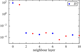
Fig.  2: The effective interactions $D(j-i)$ in a one-dimensional chain of $N=100$ impenetrable rods. Beyond nearest neighbours the interactions are zero to within statistical noise. Larger blue symbols are positive values, smaller red are symbols negative values. $K=N\times 10^{7}$ recordings, obtained from three independently simulated trajectories.

3.2 Two-dimensional crystal

We performed two-dimensional simulations in systems with $N=L{\times}L$ hard disks, $L$ varying from $10$ to $100$ with fixed surface fraction $\phi=0.85$. We expect that the elements of the effective dynamical matrix $D$ come from the local physics (and available entropy) occurring near each particle and are not the results of a non-trivial propagation of boundary effects down to the microscopic scale. If the physics is local, we then expect that the values of the elements of $D$ vary very little with changes in the system size. To test this, we plot in Fig. 3 the evolution of $\operatorname{tr}\bigl{(}D(\mathbf{n})\bigr{)}$ with the system size $L$ and find that the lines for small separations $\mathbf{n}$ are remarkably stable. This is true for all matrix elements of $D_{\alpha\beta}$, not only for the trace. Since we are performing simulations within a periodic box, it is clear that we should only be evaluating elements for separations such that periodic copies do not contaminate the result. Thus we will only quantitatively analyse $D$ for separations which are smaller than $L/2$.

The correlation function $G$, which is measured in the simulations and displayed in Fig. 1, is subject to strong finite size corrections due to the logarithmic nature of two-dimensional Green functions. The components of the matrix $D$, however, do not evolve for small values of $1/L$. From the curves in Fig. 3 we decided to use a fixed value of $L=32$ for further simulation in order to collect the highest possible statistics, while being able to resolve effective interactions out to a large distance.

Fig.  3: Effective interactions as a function of the inverse system size $1/L$. Different plot styles correspond to different neighbour layers, starting from $0$ at the top, down to $7$. Fewer layers are plotted for $L=10$.

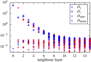
Fig.  4: Effective interactions in a hexagonal hard-disk crystal with $L=32$. Larger blue symbols are positive values, smaller red symbols are negative values. $K=2N\times 3.5{\times}10^{6}$ recordings, obtained from 336 independent trajectories. Surface fraction $\phi=0.85$. These data required around 300 000 CPU core hours.

The resulting matrix elements are plotted in Fig. 4. As we did already in Fig. 1, we rotated the $2{\times}2$ matrices $D_{\alpha\beta}(\mathbf{n})$ for each separation vector $\mathbf{R}_{\mathbf{n}}$. We used the same rotated orthonormal basis and the same notation as we used in Eqs. (9). The interaction matrix depicted in Fig. 4 does not vanish beyond the first layer of neighbours – very differently from its unidimensional counterpart in Fig. 2. We here observe that $D(\mathbf{n})$ is not sparse. We used very high statistics in this plot to be sure that the interaction data is well separated from statistical noise – We find it to be the case for the first six layers of neighbours. The noise level can be read off from the values of $D_{\text{asym}}$ which are zero in noiseless data, finding values below $2{\times}10^{-2}$. Beyond the 10th layer of neighbours, signal and noise cannot be distinguished anymore. Another measure of the statistical noise is the spread of those symbols which are equal by symmetry of the lattice (smaller than the linewidth in the plot). Both measures for the noise were observed to decrease while we accumulated more and more data during the simulations.

We tried to characterise the decay of the effective interactions with particle separation, which we can resolve out to the eighth layer of neighbours. We tried fitting the data with both exponential and power law decays, plotting both particle separation and layer number for the abscissa. No fit seemed totally convincing with our data. If one insists on fitting with a power law $\|\mathbf{R}_{\mathbf{n}}\|^{\alpha}$, one finds $\alpha\approx-6\pm 0.5$. At the moment we do not have analytic arguments that would predict the functional form of the decay.

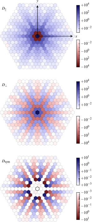
Fig.  5: Matrix elements of $D(\mathbf{n})$ in rotated frames of reference, for several $\mathbf{R}_{\mathbf{n}}$. The center of the hexagon corresponds to $\mathbf{R}_{\mathbf{n}}=\mathbf{0}$. The antisymmetric off-diagonal $D_{\text{asym}}$ vanishes to within statistical noise. The reflection anti-symmetry of $D_{sym}$ imposes that the elements of $D_{sym}$ are zero for the first two neighbour layers. All elements of $D_{sym}$ are small compared to $D_{\parallel}$ and $D_{\perp}$.

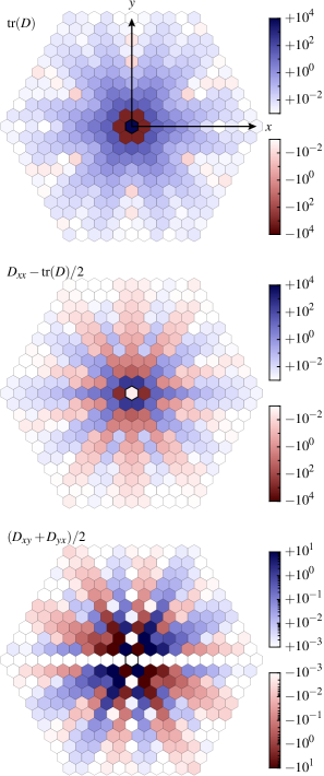
Fig.  6: Some linear combinations of matrix elements $D_{\alpha\beta}(\mathbf{n})$ for several $\mathbf{R}_{\mathbf{n}}$. The antisymmetric off-diagonal $(D_{xy}-D_{yx})/2$ vanishes to within statistical noise.

3.2.1 Two-dimensional visualisation

We now give some more details of the data presented in Fig. 4. In particular, we like to visualise those points which are characterised by being within same neighbour level, but which differ with respect to the hexagonal symmetry.

We can study the $2{\times}2$ matrices $D(\mathbf{n})$ in different frames of reference. The first frame of reference is the orthonormal basis $(\hat{\mathbf{R}}_{\mathbf{n}},\hat{\mathbf{o}})$ already used above. In Fig. 5 we plot the parallel, the orthogonal, and the off-diagonal component of the matrix. All three panels are invariant under rotations of 60 degrees. Under mirroring, however, only the first two are invariant while $D_{\text{sym}}$ changes sign. We did not plot $D_{\text{asym}}$ because it contains only noise.

A second manner of examining the data is in the fixed Cartesian frame, which is the same for all $\mathbf{n}$. In Fig. 6 we study the trace of the matrix, $\operatorname{tr}(D)$, the first component $D_{xx}$ of which we subtracted half the trace, and the off-diagonal element $D_{xy}$, symmetrised. The component $D_{yy}-\operatorname{tr}(D)/2$ is not plotted as it is simply the negative of $D_{xx}-\operatorname{tr}(D)/2$. Only $\operatorname{tr}(D)$ still has hexagonal symmetry. The two bottom panels show (skew) symmetry with respect to mirroring about the $x$-axis and the $y$-axis. We found the same skew symmetry in the Hessian matrix, Eq. (10). The special choice of component combinations in Fig. 6 is motivated by the continuum limit which we discuss now.

3.2.2 Hexagonal continuum limit

The matrix $D_{\alpha\beta}(\mathbf{n})$ is the inverse of the Green function of static elasticity and is thus expected to be related to the corresponding differential operator – or rather its hexagonal discretisation. Continuum elastic theory of pre-stressed materials gives the differential operator (Sec. 3 of Ref. 13)

$$\mathcal{D}_{\alpha\sigma}=-A_{\alpha\beta\sigma\tau}\partial_{\beta}\partial_{\tau},$$ (24)

where we have to remember that the two elastic tensors $A$ and $C$ coincide only in systems whose reference state is stress-free. The hard-sphere crystal in our numerical simulation is compressed by the periodic boundary conditions, leading to the isotropic stress $T_{\beta\tau}=-P\delta_{\beta\tau}$ with the pressure $P$. Consequently, the two tensors $A$ and $C$ are different. Assembling Eqs. (12), (14), we find the differential operator to be

$$\mathcal{D}_{\alpha\beta}=-(\mu-P)\delta_{\alpha\beta}{\boldsymbol{\nabla}}^{2}-(\lambda+\mu)\partial_{\alpha}\partial_{\beta}.$$ (25)

For these second derivatives, we can produce simple discretisations in terms of finite differences on nearest neighbours. In particular, the combinations of matrix elements used in Fig. 6 are simple combinations of second derivatives,

$$\operatorname{tr}\mathcal{D} \propto-{\boldsymbol{\nabla}}^{2}=\frac{1}{3d_{0}^{2}}\parbox{48.36967pt}{\includegraphics{eq26a}}$$ (26a)

$$\mathcal{D}_{xx}-\frac{\operatorname{tr}\mathcal{D}}{2} \propto\partial_{y}^{2}-\partial_{x}^{2}=\frac{1}{3d_{0}^{2}}\parbox{48.36967pt}{\includegraphics{eq26b}}$$ (26b)

$$\frac{\mathcal{D}_{xy}+\mathcal{D}_{yx}}{2} \propto-\frac{\partial_{x}\partial_{y}+\partial_{y}\partial_{x}}{2}=\frac{1}{\sqrt{3}d_{0}^{2}}\parbox{48.36967pt}{\includegraphics{eq26c}}$$ (26c)

We see that these stencils are qualitatively reproduced in the central parts of the panels in Fig. 6. However, Fig. 6 shows nonzero interactions also beyond the first layer of neighbours. Another difference is that for $\operatorname{tr}(D)$ we find a middle value which is $-5.6$ times the values found on the first neighbours (instead of $-6$). When comparing the values of the first neighbours among themselves, the stencils are again well reproduced, with variations as small as $\sim 10^{-5}$ in all three panels of Fig. 6. The skew symmetry of the operator $\partial_{x}\partial_{y}$ is found again in all values of $D_{xy}(\mathbf{n})$. This symmetry imposes the horizontal and the vertical white lines (zeros) in the third panel of Fig. 6.

The matrix $D_{\alpha\beta}(\mathbf{n})$ encodes the full dispersion curves that are required to determine the spectral properties of the fluctuations. In particular, one can extract the elastic tensor $A$ from the long-wavelength limit. The usual way to do this calculation is to perform a discrete periodic (fast) Fourier transform on the matrix $G_{\alpha\beta}(\mathbf{i},\mathbf{j})$ and to observe that the translation invariance renders the result block-diagonal. For each reciprocal vector $\mathbf{Q}_{\mathbf{m}}$ we have one Fourier transformed $d{\times}d$ matrix

$${\tilde{G}}_{\alpha\beta}(\mathbf{m}) :=N\sum_{\mathbf{n}}e^{-i\mathbf{Q}_{\mathbf{m}}\cdot\mathbf{R}_{\mathbf{n}}}G_{\alpha\beta}(\mathbf{n})$$ (27)

$$=\Bigl{\langle}\overline{{\tilde{u}}_{\alpha}(\mathbf{m})}{\tilde{u}}_{\beta}(\mathbf{m})\Bigr{\rangle}.$$ (28)

The overline denotes a complex conjugate. To leading order, this matrix scales as $|\mathbf{Q}_{\mathbf{m}}|^{-2}$, such that we can extract the elastic tensor as the long-wavelength prefactor to this scaling,

$$A_{\alpha\sigma\beta\tau}{\hat{Q}}_{\sigma}{\hat{Q}}_{\tau}=\frac{kT\,N^{2}}{V}\lim_{|\mathbf{Q}_{\mathbf{m}}|\to 0}\frac{\bigl{[}{\tilde{G}}(\mathbf{m})^{-1}\bigr{]}_{\alpha\beta}}{|\mathbf{Q}_{\mathbf{m}}|^{2}}.$$ (29)

In practice, rather the eigenvalues of the inverse matrix are plotted, see Fig. 7. The long-wavelength limit is then done by extrapolation by eye. The upper curve corresponds to the longitudinal waves, converging to $A_{xxxx}=(\mu-P)+(\lambda+\mu)$ in the limit $|\mathbf{Q}|\to 0$. The lower curve gives the transverse value $A_{xyxy}=\mu-P$.

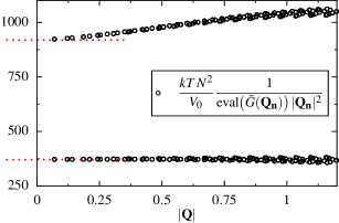
Fig.  7: Dispersion curves used to obtain the elastic moduli in the limit $|\mathbf{Q}|\to 0$, here for $L=100$. The dotted lines indicate values from a different numerical method working at $|\mathbf{Q}|=0$.

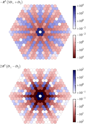
Fig.  8: The summands of Eqs. (31) and (32).

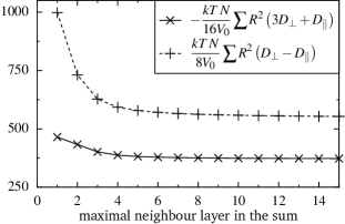
Fig.  9: Convergence of the sums in Eqs. (31) and (32).

The same limit can be done using the matrix $D$ instead of $G$. The block structure helps to invert the large matrix, the inverse is again block-diagonal. The $d{\times}d$ blocks are simply the Fourier transforms of the matrices $D_{\alpha\beta}(\mathbf{n})$: $[{\tilde{G}}(\mathbf{m})^{-1}]_{\alpha\beta}={\tilde{D}}_{\alpha\beta}(\mathbf{m})/N^{2}$. For the long-wavelength limit we expand the exponential in the definition of the Fourier transformation (27) around $\mathbf{Q}_{\mathbf{m}}=0$. The sum over the constant term vanishes, $\sum_{\mathbf{n}}D_{\alpha\beta}(\mathbf{n})=0$. The linear term vanishes due to symmetry, such that we obtain the quadratic term as the leading one. This conveniently matches with what we require for the limit in Eq. (29). Factorising the unit reciprocal vectors, we obtain for the elastic tensor

$$A_{\alpha\sigma\beta\tau}=-\frac{1}{2}\frac{kT\,N}{V}\sum_{\mathbf{n}}R_{\mathbf{n}\sigma}R_{\mathbf{n}\tau}D_{\alpha\beta}(\mathbf{n}).$$ (30)

To determine the Lam coefficients, we can either choose individual components such as $A_{xxxx}$ above, or we can do a “hexagonal average”, which amounts to reducing the rank-4 tensor to scalars, for example with $\delta_{\alpha\beta}\delta_{\sigma\tau}$ and with $\delta_{\alpha\sigma}\delta_{\beta\tau}$. This gives a $2{\times}2$ system of equations for $(\mu-P)$ and $(\lambda+\mu)$, which when solved becomes

$$\mu-P =-\frac{1}{16}\frac{kT\,N}{V}\sum_{\mathbf{n}}R_{\mathbf{n}}^{2}\bigl{(}3D_{\perp}(\mathbf{n})+D_{\parallel}(\mathbf{n})\bigr{)}$$ (31)

$$\lambda+\mu =\frac{1}{8}\frac{kT\,N}{V}\sum_{\mathbf{n}}R_{\mathbf{n}}^{2}\bigl{(}D_{\perp}(\mathbf{n})-D_{\parallel}(\mathbf{n})\bigr{)}$$ (32)

The summands are displayed in Fig. 8. They decrease with increasing distance, as expected, and their sums converge. We visualise the convergence in Fig. 9 where we added up the summands layer by layer. The final values are $\mu-P=373$ and $\lambda+\mu=553$.

In order to extract the Lam coefficients, we need also the value of the pressure $P$. During simulations, we tracked the average flux of linear momentum, which is a mechanical definition of the pressure tensor. We further measured the response of this tensor to small deformations of the simulation box, which presents another (faster converging) way to calculate the elastic moduli. Notice that this method corresponds directly to “$|\mathbf{Q}|=0$”, no limit has to be taken. We obtain the values 

$$P=34.4,\quad\mu=405,\quad\lambda=143.5\,.$$ (33)

They are used in Fig. 7 to check the consistency of the different methods. Also the values extracted from Eqs. (31) and (32) are reasonably close.

3.3 Three-dimensional crystal

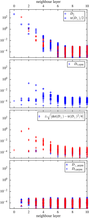
Fig.  10: Effective interactions in a FCC crystal of $N=15^{3}$ hard spheres. Larger blue symbols are positive values, smaller red symbols are negative values. $K=3N\times 6.8{\times}10^{4}$ recordings, obtained from 424 independent trajectories; volume fraction $\phi=0.57$. These data required around 230 000 CPU core hours.

We also performed simulations in three dimensions, collecting high statistics data on a system of dimensions $L=15$. Here, the result is similar to two dimensions, the effective interaction does not vanish beyond the layer of nearest neighbours but shows a rapid decrease. We adopt the same route of a rotated frame of reference to plot in Fig. 10 the matrix elements of the $3{\times}3$ matrices $D_{\alpha\beta}(\mathbf{n})$. We choose an orthonormal basis $(\hat{\mathbf{R}}_{\mathbf{n}},{\hat{\mathbf{o}}}_{1},{\hat{\mathbf{o}}}_{2})$, in which the matrix comprises the following blocks:

$$\left(\begin{array}[]{ccc}D_{\parallel}&\mathbf{v}^{T}\\ \mathbf{w}&D_{\perp}\end{array}\right)$$ (34)

As before, $D_{\parallel}=\hat{\mathbf{R}}_{\mathbf{n}}^{T}D\hat{\mathbf{R}}_{\mathbf{n}}$, but $D_{\perp}$ is a $2{\times}2$ matrix, and $\mathbf{v},\mathbf{w}$ are two-dimensional vectors. As the basis vectors ${\hat{\mathbf{o}}}_{1},{\hat{\mathbf{o}}}_{2}$ can be chosen with an arbitrary rotation about the vector $\hat{\mathbf{R}}_{\mathbf{n}}$, we are only interested in invariants of $D_{\perp},\mathbf{v},\mathbf{w}$ under this rotation. For the matrix $D_{\perp}$ we thus plot in Fig. 10 the trace of $D_{\perp}$, its anti-symmetrised off-diagonals $D_{\perp,\text{asym}}$ and some notion of its determinant. For $\mathbf{v},\mathbf{w}$ we plot the modulus after (anti)-symmetrising, $D_{v,\text{sym}}:=\|\mathbf{v}+\mathbf{w}\|/2$, $D_{v,\text{asym}}:=\|\mathbf{v}-\mathbf{w}\|/2$. The lowest panel in Fig. 10 allows one to estimate the noise level for the given statistics.

If again one insists on an algebraic fit $D(\mathbf{n})\propto\|\mathbf{R}/d_{0}\|^{\alpha}$, one finds $\alpha\approx-8\pm 1$. In three dimension the data display less scatter when plotted in terms of neighbour layer, rather than separation. This is a non-trivial geometrical effect which is already visible in two dimensions: In the first panel of Fig. 5, the values on the diagonals of the hexagon are larger than the values at the same distance (even larger than those on the same neighbour level). This creates within every neighbour level (or distance) a tendency which is opposed to the general trend.

4 Discussion and conclusions

In section 3 we have presented a number of properties, some of which are compatible, others are incompatible with the expectation elaborated from the central model in section 2. Let us now scrutinise these properties and see to what extend we can understand the differences.

4.0.0.1 Elastic moduli:

Let us start with the elastic moduli and the Cauchy relation. The values we found for the Lam coefficients in Eqs. (33) show that the two-dimensional hexagonal crystal is far from being “Cauchy”, $\mu$ being nearly three times as large as $\lambda$, where the Cauchy relations would require them to be equal. This finding is neither new¹² nor surprising, as shows the calculation by Squire et al. ¹¹, which we recapitulated in Sec. 2.3. One concludes that the non-thermal central force model is inadequate for understanding the elastic moduli of the hard-sphere system, that the kinetic term and probably more important the fluctuations term are not small, and finally that we can indeed expect the hard-sphere system to be dominated by thermal effects and to see important deviations also in the interaction matrix.

4.0.0.2 Pressure:

As a side remark, we find it an interesting question whether one can determine the pressure in a system by measuring displacements and their correlations.¹⁶ Equation (16) shows that this is indeed possible in the non-thermal model, where the pressure is minus a diagonal term of the stress in Eq. (16), or ${\bar{P}}=-\frac{N}{4V}\sum_{\mathbf{n}}R_{\mathbf{n}}^{2}g^{\prime}_{\mathbf{n}}\bigl{(}R_{\mathbf{n}}^{2}/2\bigr{)}$. The values of $g_{\mathbf{n}}^{\prime}$ are translated back to $H_{\perp}$ using Eq. (9b). Does the same work also in the thermal case, using $D_{\perp}$ instead of $H_{\perp}$? When we use the numerical data for $D_{\perp}$, shown in Fig. 5, then we find the value $-96$ for this effective pressure – which is clearly unacceptable, even the sign is wrong. In fact, a close look on Eqs. (31) and (32) reveals that the sum actually calculates $P+(\lambda-\mu)/2$ and equals the pressure only to the extent that the Cauchy relation is satisfied.

4.0.0.3 Locality of the interaction:

Independent of all questions of how the data compare to a model, we found that the correlation matrix strongly depends on the system size, whereas its inverse does not (Fig. 3). Our intuition, in which we called the correlations a “Green function” and its inverse a “differential operator” heavily relies on a clear-cut separation of size dependence. We find that the differential operator ($D$) is indeed “local”, but the precise notion of this locality is different in one and in higher dimensions. In one dimension we find the interaction matrix to be restricted to the two nearest neighbours, as expected from a Laplace operator. In two and three dimensions the results are much more interesting: Despite the true interactions taking place to nearest neighbours, we find longer-ranged effective interactions from the analysis of displacement correlations. These interactions are small compared to the ones between nearest neighbours, but they are not exactly zero and can be distinguished from noise. It remains open what functional form the decrease in Figs. 4 and 10 follows, and whether an algebraic form would still allow to reasonably call the operator “local.”

4.0.0.4 Theoretical interpretation of the dynamic matrix as a self-energy:

The presented results open the question of a better theoretical interpretation than the one in Sec. 2.1. In particular one would like to predict how the effective interactions decay with distance. It is clear that in a field-theory formulation of a perturbed Gaussian theory the effective interactions $D$ correspond to the self-energy in a Dyson equation. However, without an explicit perturbation scheme for hard sphere systems it is difficult to turn this remark into an explicit calculation.

4.0.0.5 Nonlinearities in the interaction potential:

Getting back to the central-force model of Sec. 2.1, it does not favour local or nonlocal interactions in its general form. If we want more information, we need to specify the functions $g_{\mathbf{i}\mathbf{j}}$. One choice is to take the true hard-sphere interactions, the pair potential being either zero or infinity. Around the reference state, the potential is zero, together with its first and second derivative. Therefore, the Hessian matrix vanishes, and also the stress and elastic tensors consist only in the kinetic terms. Here, the model is clearly out of its applicability.

We learn from this remark that the model equations do not necessarily serve to infer the true interaction between particles from given data. But, what lesson do we want to learn from the model? Our aim was to contrast thermal with respect to non-thermal effects. Unfortunately, in the hard-sphere simulations, together with thermal effects, we introduced strong nonlinearities in the pair potential. Now we have a hard time to separate their influence from the thermal effects. (At least in the elastic constants, the nonlinearities play no role, which is reassuring.)

Another convenient choice for the functions $g_{\mathbf{i}\mathbf{j}}$ is a network of linear springs which have zero length at rest. When such a network is stretched, the particles may be found on a hexagonal reference lattice. In this system the Hessian matrix is a constant, and all statistical averages are Gaussian integrals which can be solved analytically via Wick’s theorem. The effective interactions are indeed found to be given by the Hessian matrix, $D=H/kT$, which in turn is given by the connections of particles. If we choose to have identical springs between nearest neighbours only, then also the matrix $D$ is restricted to nearest neighbours. The same applies to second-nearest neighbours, and so on. One might think that this linear system will help to differentiate between thermal and nonlinear effects. However, when one evaluates the averages in Eq. (19), which contains all thermal effects, one finds that the elastic tensor is zero. The zero-length spring network is thus not good enough to separate nonlinear from thermal effects.

If we insist on central pair potentials, the zero-length spring network is the only linear one we know of. Of course, other arbitrary linear models can be created by choosing a potential of the form (3), i. e. exactly quadratic in the displacements – one can even take the measured matrix $D$ as the matrix in this expression, which amounts to the shadow system of Ref. 7. However, doing so one relaxes the constraint of the central potential and includes knowledge about the reference positions in the potential. Moreover, by construction the shadow system has the same displacement correlations, the same interaction matrix, and the same elastic constants as the original system. Only higher-order correlations differ. We are thus back to the question what do we want to learn from comparing with a model? Should it contain information about the reference positions, thus about the spontaneous symmetry breaking or not?

Another possible approach to a model would consist in extracting the “best” central-force model from the numerical data. Wanted is a discrete function $g_{\mathbf{n}}$ of which the first and second derivatives are given by $g_{\mathbf{n}}^{\prime}=-D_{\perp}(\mathbf{n})$ and $g_{\mathbf{n}}^{\prime\prime}=\bigl{(}D_{\perp}(\mathbf{n})-D_{\parallel}(\mathbf{n})\bigr{)}/R_{\mathbf{n}}^{2}$, respectively – in the hexagonal case, in analogy to Eqs. (9a) and (9b). The first derivative can be read off Fig. 5, and the second one is given up to a factor $R_{\mathbf{n}}^{4}$ in the lower panel of Fig. 8. We did not try to perform this extraction and do not know whether the problem has a unique solution or approximation methods are required.

4.0.0.6 Non-central forces:

The main lesson we can learn from the comparison with the model is probably that the effective interactions contained in $D$ are non-central: It is striking that $H_{\text{sym}}(\mathbf{n})$ is identically zero for all $\mathbf{n}$, whereas $D_{\text{sym}}(\mathbf{n})$ has nonzero values. The thermal interactions are thus genuinely non-central. We note that the off-diagonal term $D_{\text{sym}}(\mathbf{n})$ is smaller in amplitude than the terms on the diagonal, $D_{\parallel}$ and $D_{\perp}$, so that the non-central nature can be considered a correction to the dominant terms.

References

- Ghosh et al. 2011 A. Ghosh, R. Mari, V. Chikkadi, P. Schall, A. Maggs and D. Bonn, Physica A: Statistical Mechanics and its Applications, 2011, 390, 3061 – 3068.
- Ghosh et al. 2010 A. Ghosh, V. K. Chikkadi, P. Schall, J. Kurchan and D. Bonn, Phys. Rev. Lett., 2010, 104, 248305.
- Chen et al. 2013 K. Chen, T. Still, S. Schoenholz, K. B. Aptowicz, M. Schindler, A. C. Maggs, A. J. Liu and A. G. Yodh, Phys. Rev. E, 2013, 88, 022315.
- Yunker et al. 2014 P. J. Yunker, K. Chen, M. D. Gratale, M. A. Lohr, T. Still and A. G. Yodh, Reports on Progress in Physics, 2014, 77, 056601.
- Underwood et al. 1994 S. M. Underwood, J. R. Taylor and W. van Megen, Langmuir, 1994, 10, 3550–3554.
- Brito et al. 2010 C. Brito, O. Dauchot, G. Biroli and J.-P. Bouchaud, Soft Matter, 2010, 6, 3013–3022.
- Henkes et al. 2012 S. Henkes, C. Brito and O. Dauchot, Soft Matter, 2012, 8, 6092–6109.
- Chen et al. 2010 K. Chen, W. G. Ellenbroek, Z. Zhang, D. T. N. Chen, P. J. Yunker, S. Henkes, C. Brito, O. Dauchot, W. van Saarloos, A. J. Liu and A. G. Yodh, Phys. Rev. Lett., 2010, 105, 025501.
- Lemarchand et al. 2012 C. A. Lemarchand, A. C. Maggs and M. Schindler, EPL (Europhysics Letters), 2012, 97, 48007.
- Born and Huang 1998 M. Born and K. Huang, Dynamical Theory of Crystal Lattices, Oxford University Press, Oxford, 1998.
- Squire et al. 1969 D. Squire, A. Holt and W. Hoover, Physica, 1969, 42, 388 – 397.
- Wojciechowski et al. 2003 K. W. Wojciechowski, K. V. Tretiakov, A. C. Brańka and M. Kowalik, The Journal of Chemical Physics, 2003, 119, 939–946.
- Wallace 1970 D. C. Wallace, in Thermoelastic Theory of Stressed Crystals and Higher-Order Elastic Constants, ed. H. Ehrenreich, F. Seitz and D. Turnbull, Academic Press, New York and London, 1970, vol. 25, pp. 301–404.
- Barnes and Kofke 1999 C. D. Barnes and D. A. Kofke, The Journal of Chemical Physics, 1999, 110, 11390–11398.
- Sengupta et al. 2000 S. Sengupta, P. Nielaba, M. Rao and K. Binder, Phys. Rev. E, 2000, 61, 1072–1080.
- 16 D. Bonn, private communication.