Recognizing and Drawing IC-planar Graphs

Abstract

We give new results about the relationship between 1-planar graphs and RAC graphs. A graph is 1-planar if it has a drawing where each edge is crossed at most once. A graph is RAC if it can be drawn in such a way that its edges cross only at right angles. These two classes of graphs and their relationships have been widely investigated in the last years, due to their relevance in application domains where computing readable graph layouts is important to analyze or design relational data sets. We study IC-planar graphs, the sub-family of 1-planar graphs that admit 1-planar drawings with independent crossings (i.e., no two crossed edges share an endpoint). We prove that every IC-planar graph admits a straight-line RAC drawing, which may require however exponential area. If we do not require right angle crossings, we can draw every IC-planar graph with straight-line edges in linear time and quadratic area. We then study the problem of testing whether a graph is IC-planar. We prove that this problem is NP-hard, even if a rotation system for the graph is fixed. On the positive side, we describe a polynomial-time algorithm that tests whether a triangulated plane graph augmented with a given set of edges that form a matching is IC-planar.

1 Introduction

Graph drawing is a well-established research area that studies how to automatically compute visual representations of relational data sets in many application domains, including software engineering, circuit design, computer networks, database design, social sciences, and biology (see, e.g., [16, 22, 37, 38, 48, 49]). The aim of a graph visualization is to clearly convey the structure of the data and their relationships, in order to support users in their analysis tasks. In this respect, there is a general consensus that edges with many crossings and bends negatively affect the readability of a drawing of a graph, as also witnessed by several user studies on the subject (see, e.g., [45, 46, 52]). At the same time, more recent cognitive experiments suggest that edge crossings do not inhibit user task performance if the edges cross at large angles [33, 34, 36]. As observed in [21], intuitions of this fact can be found in real-life applications: for example, in hand-drawn metro maps and circuit schematics, where edge crossings are conventionally at 90 degrees (see, e.g., [51]), and in the guidelines of the CCITT (Comité Consultatif International Téléphonique et Télégraphique) for drawing Petri nets, where it is written: “There should be no acute angles where arcs cross” [13].

The above practical considerations naturally motivate the theoretical study of families of graphs that can be drawn with straight-line edges, few crossings per edge, and right angle crossings at the same time. This kind of research falls in an emerging topic of graph drawing and graph theory, informally called “beyond planarity”. The general framework of this topic is to relax the planarity constraint by allowing edge crossings, but still forbidding those configurations that would affect the readability of the drawing too much. Different types of forbidden edge-crossing configurations give rise to different families of beyond planar graphs. For example, for any integer $k\geq 3$, the family of $k$-quasi planar graphs is the set of graphs that have a drawing with no $k$ mutually crossing edges (see, e.g., [1, 2, 28]). For any positive integer $k$, the family of $k$-planar graphs is the set of graphs that admit a drawing with at most $k$ crossings per edge [43]; in particular, $1$-planar graphs have been widely studied in the literature (see, e.g., [3, 20, 30, 32, 39, 47]). RAC (Right Angle Crossing) graphs are those graphs that admit a drawing where edges cross only at right angles (see, e.g., [21]). Several algorithms and systems for computing RAC drawings or, more in general, large angle crossing drawings, have been described in the literature (see, e.g., [5, 17, 18, 19, 24, 25, 42, 35]). See also [23] for a survey.

In this scenario, special attention is receiving the study of the relationships between 1-planar drawings and RAC drawings with straight-line edges. The maximum number of edges of an $n$-vertex 1-planar graph is $4n-8$ [43], while $n$-vertex straight-line 1-planar drawings and $n$-vertex straight-line RAC drawings have at most $4n-9$ edges [20] and $4n-10$ edges [21], respectively. This implies that not all 1-planar graphs admit a straight-line drawing and not all 1-planar graphs with a straight-line drawing admit a straight-line RAC drawing. The characterization of the 1-planar graphs that can be drawn with straight-line edges was given by Thomassen in 1988 [50].

Our Contribution. In this paper we give new results on the relationship between 1-planar graphs, RAC graphs, and straight-line drawings. We concentrate on a subfamily of 1-planar graphs known as IC-planar graphs, which stands for graphs with independent crossings [4]. An IC-planar graph is a graph that admits a 1-planar drawing where no two crossed edges share an endpoint, i.e., all crossing edges form a matching. IC-planar graphs have been mainly studied both in terms of their structure and in terms of their applications to coloring problems [4, 40, 53, 54]. We prove that:

• Every IC-planar graph with $n$ vertices admits a (non-RAC) straight-line drawing in $O(n^{2})$ area, which can be computed in $O(n)$ time (Theorem 1). Our bound on the area requirement is worst-case optimal. We recall that there are embedded 1-planar graphs whose straight-line drawings require $\Omega(2^{n})$ area [32].

• Every IC-planar graph is a RAC graph (Theorem 2), but we also show that a straight-line RAC drawing of an $n$-vertex IC-plane graph may require $\Omega(q^{n})$ area, for a suitable constant $q>1$ (Theorem 3).

Moreover, as a natural problem related to the results above, we study the computational complexity of recognizing IC-planar graphs. Namely:

• We prove that IC-planarity testing is $\mathrm{NP}$-complete both in the variable embedding setting (Theorem 4) and when the rotation system of the graph is fixed (Theorem 5). Note that, 1-planarity testing is already known to be $\mathrm{NP}$-complete in general [30, 39] and for a fixed rotation system [7]. Testing 1-planarity remains NP-hard even for near-planar graphs, i.e., graphs that can be obtained by a planar graph by adding an edge [11].

• On the positive side, we give a polynomial-time algorithm that tests whether a triangulated plane graph augmented with a given set of edges that form a matching is IC-planar (Theorem 6). The interest in this special case is also motivated by the fact that every $n$-vertex IC-planar graph with maximum number of edges (i.e., with $13n/4-6$ edges) is the union of a triangulated planar graph and of a set of edges that form a matching [54].

We finally recall that the problem of recognizing 1-planar graphs has been studied also in terms of parameterized complexity. Namely, Bannister, Cabello, and Eppstein describe fixed-parameter tractable algorithms with respect to different parameters: vertex cover number, tree-depth, and cyclomatic number [8]. They also show that the problem remains NP-complete for graphs of bounded bandwidth, pathwidth, and treewidth, which makes unlikely to find parameter tractable algorithms with respect to these parameters. Fixed-parameter tractable algorithms have been also described for computing the crossing number of a graph, a problem that is partially related to the research on beyond planarity (see, e.g., [31, 44]).

The remainder of the paper is organized as follows. In Section 2 we recall basic definitions used in the paper. Section 3 is devoted to prove Theorem 1. In Section 4 we prove Theorems 2 and 3. Section 5 proves Theorems 4, 5, and 6. Conclusions and open problems are in Section 6.

2 Preliminaries

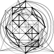
Figure 1: (a) An IC-planar drawing. (b) Two different IC-planar embeddings of the same graph with the same rotation system. (c) An X-configuration. (d) A B-configuration.

We consider simple undirected graphs $G$. A drawing $\Gamma$ of $G$ maps the vertices of $G$ to distinct points in the plane and the edges of $G$ to simple Jordan curves between their endpoints. If the vertices are drawn at integer coordinates, $\Gamma$ is a grid drawing. $\Gamma$ is planar if no edges cross, and 1-planar if each edge is crossed at most once. $\Gamma$ is IC-planar if it is 1-planar and there are no crossing edges that share a vertex. An example of an IC-planar graph is shown in Figure 1.

A planar drawing $\Gamma$ of a graph $G$ induces an embedding, which is the class of topologically equivalent drawings. In particular, an embedding specifies the regions of the plane, called faces, whose boundary consists of a cyclic sequence of edges. The unbounded face is called the outer face. For a 1-planar drawing, we can still derive an embedding by allowing the boundary of a face to consist also of edge segments from a vertex to a crossing point. A graph with a given planar (1-planar, IC-planar) embedding is called a plane (1-plane, IC-plane) graph. A rotation system $\mathcal{R}(G)$ of a graph $G$ describes a possible cyclic ordering of the edges around the vertices. $\mathcal{R}(G)$ is planar (1-planar, IC-planar) if $G$ admits a planar (1-planar, IC-planar) embedding that preserves $\mathcal{R}(G)$. Observe that $\mathcal{R}(G)$ can directly be retrieved from a drawing or an embedding. The converse does not necessarily hold, as shown in Figure 1.

A kite $K$ is a graph isomorphic to $K_{4}$ with an embedding such that all the vertices are on the boundary of the outer face, the four edges on the boundary are planar, and the remaining two edges cross each other; see Figure 1. Thomassen [50] characterized the possible crossing configurations that occur in a 1-planar drawing. Applying this characterization to IC-planar drawings gives rise to the following property:

Property 1.

Every crossing of an IC-planar drawing is either an X- or a B-crossing.

Here, an X-crossing has the crossing “inside” the 4-cycle (see Figure 1), and a B-crossing has the crossing “outside” the 4-cycle (see Figure 1). We remark that, according to Thomassen [50], a $1$-planar drawing may contain crossings that are neither X- nor B-crossings, but W-crossings. This third type of crossing is not possible in an IC-planar drawing since it contains two vertices incident to two crossed edges.

Let $G$ be a plane (1-plane, IC-plane) graph. $G$ is maximal if no edge can be added without violating planarity (1-planarity, IC-planarity). A planar (1-planar, IC-planar) graph $G$ is maximal if every planar (1-planar, IC-planar) embedding is maximal. If we restrict to 1-plane (IC-plane) graphs, we say that $G$ is plane-maximal if no edge can be added without creating at least an edge crossing on the newly added edge (or making the graph not simple). We call the operation of adding edges to $G$ until it becomes plane-maximal a plane-maximal augmentation.

3 Straight-line drawings of IC-planar graphs

We show that every IC-planar graph admits an IC-planar straight-line grid drawing in quadratic area, and this area is worst-case optimal (Theorem 1). The result is based on first using a new technique that augments an embedding of the input graph to a maximal IC-plane graph (the resulting embedding might be different from the original one) with specific properties (Lemma 1), and then suitably applying a drawing algorithm by Alam et al. for triconnected 1-plane graphs [3] on the augmented graph. We say that a kite $(a,b,c,d)$ with crossing edges $(a,d)$ and $(b,c)$ is empty if it contains no other vertices, that is, the edges $(a,c)$, $(a,d)$, and $(a,b)$ are consecutive in the counterclockwise order around $a$; see Figure 2(b). The condition for the edges around $b$, $c$, and $d$ is analogous. We are now ready to prove the next lemma.

Lemma 1.

Let $G=(V,E)$ be an IC-plane graph with $n$ vertices. There exists an $O(n)$-time algorithm that computes a plane-maximal IC-plane graph $G^{+}=(V,E^{+})$ with $E\subseteq E^{+}$ such that the following conditions hold:

1. The four endpoints of each pair of crossing edges induce a kite.

2. Each kite is empty.

3. Let $C$ be the set of crossing edges in $G^{+}$. Let $C^{*}\subset C$ be a subset containing exactly one edge for each pair of crossing edges. Then $G^{+}\setminus C^{*}$ is plane and triangulated.

4. The outer face of $G^{+}$ is a $3$-cycle of non-crossed edges.

(a) The kite (drawn bold) is not empty

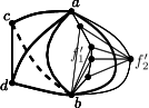
(b) Rerouting edge $(a,b)$ to make the kite empty

(c) Triangulating the remaining faces

Figure 2: Illustration for the proof of Lemma 1.

Proof.

Let $G$ be an IC-plane graph; we augment $G$ by adding edges such that for each pair of crossing edges $(a,d)$ and $(b,c)$ the subgraph induced by vertices $\{a,b,c,d\}$ is isomorphic to $K_{4}$; see the dashed edges in Figures 1 and 1. Next, we want to make sure that this subgraph forms an X-configuration and the resulting kite is empty. Since $G$ is IC-planar, it has no two B-configurations sharing an edge. Thus, we remove a B-configuration with vertices $\{a,b,c,d\}$ by rerouting the edge $(a,b)$ to follow the edge $(a,d)$ from vertex $a$ until the crossing point, then edge $(b,c)$ until vertex $b$, as shown by the dotted edge in Figure 1. This is always possible, because edges $(a,c)$ and $(b,d)$ only cross each other; hence, following their curves, we do not introduce any new crossing. The resulting IC-plane graph satisfies (c1) (recall that, by Property 1, only X- and B-configurations are possible). Now, assume that a kite $(a,b,c,d)$ is not empty; see Figure 2(a). Following the same argument as above, we can reroute the edges $(a,b)$, $(b,d)$, $(c,d)$ and $(a,d)$ to follow the crossing edges $(a,d)$ and $(b,c)$; see Figure 2(b). The resulting IC-plane graph is denoted by $G^{\prime}$ and satisfies (c2).

We now augment $G^{\prime}$ to $G^{+}$, such that (c3) is satisfied. Let $C$ be the set of all pairs of crossing edges in $G^{\prime}$. Let $C^{*}$ be a subset constructed from $C$ by keeping only one (arbitrary) edge for each pair of crossing edges. The graph $G^{\prime}\setminus C^{*}$ is clearly plane. To ensure (c3), graph $G^{+}\setminus C^{*}$ must be plane and triangulated. Because $G^{\prime}$ satisfies (c2), each removed edge spans two triangular faces in $G^{\prime}\setminus C^{*}$. Thus, no face incident to a crossing edge has to be triangulated. We internally triangulate the other faces by picking any vertex on its boundary and connecting it to all other vertices (avoiding multiple edges) of the boundary; see e.g. Figure 2(c). Graph $G^{+}$ is then obtained by reinserting the edges in $C^{*}$ and satisfies (c3). To satisfy (c4), notice that $G^{+}$ is IC-plane, hence, it has a face $f$ whose boundary contains only non-crossed edges. Also, $f$ is a $3$-cycle by construction. Thus, we can re-embed $G^{+}$ such that $f$ is the outer face.

It remains to prove that the described algorithm runs in $O(n)$ time. Let $m$ be the number of edges of $G$. Augmenting the graph such that for each pair of crossing edges their endpoints induce a subgraph isomorphic to $K_{4}$ can be done in $O(m)$ time (the number of added edges is $O(n)$). Similarly, rerouting some edges to remove all B-configurations requires $O(m)$ time. Also, triangulating the graph $G^{\prime}\setminus C^{*}$ can be done in time proportional to the number of faces of $G^{\prime}\setminus C^{*}$, which is $O(n+m)$. Since IC-planar graphs are sparse [54], the time complexity follows. ∎

Theorem 1.

There is an $O(n)$-time algorithm that takes an IC-plane graph $G$ with $n$ vertices as input and constructs an IC-planar straight-line grid drawing of $G$ in $O(n)\times O(n)$ area. This area is worst-case optimal.

Proof.

Augment $G$ into a plane-maximal IC-plane graph $G^{+}$ in $O(n)$ time using Lemma 1. Graph $G^{+}$ is triconnected, as it contains a triangulated plane subgraph. Draw $G^{+}$ with the algorithm by Alam et al. [3] which takes as input a 1-plane triconnected graph with $n$ vertices and computes a 1-planar drawing on the $(2n-2)\times(2n-3)$ grid in $O(n)$ time; this drawing is straight-line, but for the outer face, which may contain a bent edge if it has two crossing edges. Since by Lemma 1 the outer face of $G^{+}$ has no crossed edges, $\Gamma$ is straight-line and IC-planar. The edges added during the augmentation are removed from $\Gamma$.

It remains to prove that the area bound of the algorithm is worst-case optimal. To this aim, we show that for every $n\geq 2$ there exists an IC-planar graph $G$ with $\Theta(n)$ vertices, such that every IC-planar straight-line grid drawing of $G$ requires $\Omega(n^{2})$ area. Dolev et al. [26] described an infinite family of planar graphs, called nested triangle graphs, such that every planar straight-line drawing of an $n$-vertex graph $G$ (for $n\geq 6$) of this family requires $\Omega(n^{2})$ area. We augment $G$ as follows. For every edge $(u,v)$ of $G$, we add a vertex $c_{uv}$, and two edges $(u,c_{uv})$ and $(c_{uv},v)$. Denote by $G^{+}$ the resulting augmented graph, which clearly has $\Theta(n)$ vertices. We now show that in every possible IC-planar straight-line drawing of $G^{+}$ there are no two edges of $G$ that cross each other. Observe that the subgraph induced by the vertices $u,v,c_{uv}$ is a 3-cycle. Any drawing of two cycles must cross an even number of times. If two edges $(u,v)$ and $(w,z)$ of $G$ cross each other in an IC-planar drawing of $G^{+}$, then the cycles $u,v,c_{uv}$ and $w,z,c_{wz}$ must cross at least twice. Since these are 3-cycles, either some edge is crossed at least twice or two adjacent edges are crossed. In either case, this violates the IC-planar condition. Hence, the subgraph $G$ must be drawn planar and this implies that any straight-line IC-planar drawing of $G^{+}$ requires $\Omega(n^{2})$ area. ∎

4 IC-planarity and RAC graphs

It is known that every $n$-vertex maximally dense RAC graph (i.e., RAC graph with $4n-10$ edges) is 1-planar, and that there exist both 1-planar graphs that are not RAC and RAC graphs that are not 1-planar [27]. Here, we further investigate the intersection between the classes of 1-planar and RAC graphs, showing that all IC-planar graphs are RAC. To this aim, we describe a polynomial-time constructive algorithm. The computed drawings may require exponential area, which is however worst-case optimal; indeed, we exhibit IC-planar graphs that require exponential area in any possible IC-planar straight-line RAC drawing. Our construction extends the linear-time algorithm by de Fraysseix et al. [15] that computes a planar straight-line grid drawing of a maximal (i.e., triangulated) plane graph in quadratic area; we call it the dFPP algorithm. We need to recall the idea behind dFPP before describing our extension.

Algorithm dFPP. Let $G$ be a maximal plane graph with $n\geq 3$ vertices. The dFPP algorithm first computes a suitable linear ordering of the vertices of $G$, called a canonical ordering of $G$, and then incrementally constructs a drawing of $G$ using a technique called shift method. This method adds one vertex per time, following the computed canonical ordering and shifting vertices already in the drawing when needed. Namely, let $\sigma=(v_{1},v_{2},\dots,v_{n})$ be a linear ordering of the vertices of $G$. For each integer $k\in[3,n]$, denote by $G_{k}$ the plane subgraph of $G$ induced by the $k$ vertices $v_{1},v_{2},\dots,v_{k}$ ($G_{n}=G$) and by $C_{k}$ the boundary of the outer face of $G_{k}$, called the contour of $G_{k}$. Ordering $\sigma$ is a canonical ordering of $G$ if the following conditions hold for each integer $k\in[3,n]$: (i) $G_{k}$is biconnected and internally triangulated; (ii) $(v_{1},v_{2})$is an outer edge of $G_{k}$; and (iii) if $k+1\leq n$, vertex $v_{k+1}$ is located in the outer face of $G_{k}$, and all neighbors of $v_{k+1}$ in $G_{k}$ appear on $C_{k}$ consecutively.

We call lower neighbors of $v_{k}$ all neighbors $v_{j}$ of $v_{k}$ for which $j<k$. Following the canonical ordering $\sigma$, the shift method constructs a drawing of $G$ one vertex per time. The drawing $\Gamma_{k}$ computed at step $k$ is a drawing of $G_{k}$. Throughout the computation, the following invariants are maintained for each $\Gamma_{k}$, with $3\leq k\leq n$: (I1) $p_{v_{1}}=(0,0)$and $p_{v_{2}}=(2k-4,0)$; (I2) $x(w_{1})<x(w_{2})<\dots<x(w_{t})$, where $w_{1}=v_{1},w_{2},\dots,w_{t}=v_{2}$ are the vertices that appear along $C_{k}$, going from $v_{1}$ to $v_{2}$. (I3) Each edge $(w_{i},w_{i+1})$ (for $i=1,2,\dots,t-1$) is drawn with slope either $+1$ or $-1$.

More precisely, $\Gamma_{3}$ is constructed placing $v_{1}$ at $(0,0)$, $v_{2}$ at $(2,0)$, and $v_{3}$ at $(1,1)$. The addition of $v_{k+1}$ to $\Gamma_{k}$ is executed as follows. Let $w_{p},w_{p+1},\dots,w_{q}$ be the lower neighbors of $v_{k+1}$ ordered from left to right. Denote by $\mu(w_{p},w_{q})$ the intersection point between the line with slope $+1$ passing through $w_{p}$ and the line with slope $-1$ passing through $w_{q}$. Point $\mu(w_{p},w_{q})$ has integer coordinates and thus it is a valid placement for $v_{k+1}$. With this placement, however, $(v_{k+1},w_{p})$ and $(v_{k+1},w_{q})$ may overlap with  $(w_{p},w_{p+1})$ and $(w_{q-1},w_{q})$, respectively; see Figure 3. To avoid this, a shift operation is applied: $w_{p+1}$, $w_{p+2}$,$\dots$,$w_{q-1}$ are shifted to the right by 1 unit, and $w_{q},w_{q+1},\dots,w_{t}$ are shifted to the right by 2 units. Then $v_{k+1}$ is placed at point $\mu(w_{p},w_{q})$ with no overlap; see Figure 3. We recall that, to keep planarity, when the algorithm shifts a vertex $w_{i}$ ($p+1\leq i\leq t$) of $C_{k}$, it also shifts some of the inner vertices together with it; for more details on this point refer to [12, 15]. By Invariants (I1) and (I3), the area of the final drawing is $(2n-4)\times(n-2)$.

Figure 3: Illustration of the shift algorithm at the addition step of $v_{k+1}$. The shift operation changed the slopes of the edges drawn bold. (a) Placing $v_{k+1}$ at $\mu(w_{p},w_{q})$ would create overlaps. (b) After the shift operation, $v_{k+1}$ can be placed at $\mu(w_{p},w_{q})$ without overlaps.

Our extension. Let $G$ be an IC-plane graph, and assume that $G^{+}$ is the plane-maximal IC-plane graph obtained from $G$ by applying the technique of Lemma 1. Our drawing algorithm computes an IC-planar drawing of $G^{+}$ with right angle crossings, by extending algorithm dFPP. It adds to the classical shift operation move and lift operations to guarantee that one of the crossing edges of a kite is vertical and the other is horizontal. We now give an idea of our technique, which we call RAC-drawer. Details are given in the proof of Theorem 2. Let $\sigma$ be a canonical ordering constructed from the underlying maximal plane graph of $G^{+}$. Vertices are incrementally added to the drawing, according to $\sigma$, following the same approach as for dFPP. However, suppose that $K=(a,b,c,d)$ is a kite of $G^{+}$, and that $a$ and $d$ are the first and the last vertex of $\sigma$ among the vertices in $K$, respectively. Once $d$ has been added to the drawing, the algorithm applies a suitable combination of move and lift operations to the vertices of the kite to rearrange their positions so to guarantee a right angle crossing. Note that, following the dFPP technique, $a$ was placed at a $y$-coordinate smaller than the $y$-coordinate of $d$. A move operation is then used to shift $d$ horizontally to the same $x$-coordinate as $a$ (i.e., $(a,d)$ becomes a vertical segment in the drawing); a lift operation is used to vertically shift the lower between $b$ and $c$, such that these two vertices get the same $y$-coordinates. Both operations are applied so to preserve planarity and to maintain Invariant (I3) of dFPP; however, they do not maintain Invariant (I1), thus the area can increase more than in the dFPP algorithm and may be exponential. The application of move/lift operations on the vertices of two distinct kites do not interfere each other, as the kites do not share vertices in an IC-plane graph. The main operations of the algorithm are depicted in Figure 4.

Theorem 2.

Let $G$ be an IC-plane graph with $n$ vertices. There exists an $O(n^{3})$-time algorithm that constructs a straight-line IC-plane RAC grid drawing of $G$.

Proof.

Let $G^{+}$ be the augmented graph constructed from $G$ by using Lemma 1. Call $G^{\prime}$ the subgraph obtained from $G^{+}$ by removing one edge from each pair of crossing edges; $G^{\prime}$ is a maximal plane graph (see condition (c3) of Lemma 1). We apply on $G^{\prime}$ the shelling procedure used by de Fraysseix et al. to compute a canonical ordering $\sigma$ of $G^{\prime}$ in $O(n)$ time [14]; it goes backwards, starting from a vertex on the outer face of $G^{\prime}$ and successively removing a vertex per time from the current contour. However, during this procedure, some edges of $G^{\prime}$ can be replaced with some other edges of $G^{+}$ that were previously excluded, although $G^{\prime}$ remains maximal planar. Namely, whenever the shelling procedure encounters the first vertex $d$ of a kite $K=(a,b,c,d)$, it marks $d$ as $\operatorname{top}(K)$, and considers the edge $e$ of $K$ that is missing in $G^{\prime}$. If $e$ is incident to $d$ in $K$, the procedure reinserts it and removes from $G^{\prime}$ the other edge of $K$ that crosses $e$ in $G^{+}$. If $e$ is not incident to $d$, the procedure continues without varying $G^{\prime}$. We say that $u\prec v$ if $\sigma(u)<\sigma(v)$.

We then compute a drawing of $G^{+}$ by using the RAC-drawer algorithm. Let vertex $v=v_{k+1}$ be the next vertex to be placed according to $\sigma$. Let $\mathcal{U}(v)$ be the set of lower neighbors of $v$, and let $\lambda(v)$ and $\rho(v)$ be the leftmost and the rightmost vertex in $\mathcal{U}(v)$, respectively. Also, denote by $\mathcal{A}_{l}(v)$ the vertices to the top-left of $v$, and by $\mathcal{A}_{r}(v)$ the vertices to the top-right of $v$. If $v$ is not $\operatorname{top}(K)$ for some kite $K$, then $v$ is placed by following the rules of dFPP, that is, at the intersection of the $\pm 1$ diagonals through $\lambda(v)$ and $\rho(v)$ after applying a suitable shift operation. If $v=\operatorname{top}(K)$ for some kite $K$, the algorithm proceeds as follows. Let $K=(a,b,c,d)$ with $v=d=\operatorname{top}(K)$. The remaining three vertices of $K$ are in $G_{k}$ and are consecutive along the contour $C_{k}$, as they all belong to $\mathcal{U}(d)$ (by construction, $G^{\prime}$ contains edge $(a,d)$). W.l.o.g., assume that they are encountered in the order $\{b,a,c\}$ from left to right. The following cases are now possible:

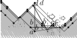
Figure 4: (a-b) The lift operation: (a) Vertex $b$ is $r$ units below $c$. (b) Lifting $b$. (c-d) The move operation: (c) Vertex $d$ is $s$ units to the left of $b$. (d) Moving $d$.

Case 1: $a\prec b$ and $a\prec c$. This implies that $a=\rho(b)$ and $a=\lambda(c)$. The edges $(a,b)$ and $(a,c)$ have slope $-1$ and $+1$, respectively, as they belong to $C_{k}$. We now aim at having $b$ and $c$ at the same $y$-coordinate, by applying a lift operation. Suppose first that $r=y(c)-y(b)>0$; see Figure 4. We apply the following steps: (i) Temporarily undo the placement of $b$ and of all vertices in $\mathcal{A}_{l}(b)$. (ii) Apply the shift operation to vertex $\rho(b)=a$ by $2r$ units to the right, which implies that the intersection of the diagonals through $\lambda(b)$ and $\rho(b)$ is moved by $r$ units to the right and by $r$ units above their former intersection point. Hence, $b$ and $c$ are placed at the same $y$-coordinate; see also Figure 4. (iii) Reinsert the vertices of $\mathcal{A}_{l}(b)$ and modify $\sigma$ accordingly. Namely, by definition, each vertex in $\mathcal{A}_{l}(b)$ does not belong to $\mathcal{U}(b)$ and it is not an inner vertex below $b$; therefore, vertices in $\mathcal{A}_{l}(b)$ can be safely removed. Hence, $\sigma$ can be modified such that $b\prec w$ for each $w\in A_{l}(b)$. If $r=y(c)-y(b)<0$, a symmetric operation is applied: (i) Undo the placement of $c$ and of all vertices in $\mathcal{A}_{r}(c)$. (ii) Apply the shift operation to vertex $\rho(c)$ by $|2r|$ additional units to the right. (iii) Reinsert the vertices of $\mathcal{A}_{r}(c)$.

Finally, we place $d$ vertically above $a$. To this aim, we first apply the shift operation according to the insertion step of dFPP. After that, we may need to apply a move operation; see Figure 4. If $s=x(d)-x(a)>0$, then we apply the shift operation to vertex $\rho(d)=c$ by $2s$ units to the right and then place $d$ (see Figure 4). If $s=x(d)-x(a)<0$, then we apply the shift operation to vertex $\lambda(d)=b$ by $2s$ units to the left and then place $d$ (clearly, the shift operation can be used to operate in the left direction with a procedure that is symmetric to the one that operates in the right direction). Edges $(a,d)$ and $(b,c)$ are now vertical and horizontal, respectively. In the next steps, their slopes do not change, as their endpoints are shifted only horizontally (they do not belong to other kites); also, $a$ is shifted along with $d$, as it belongs to $\mathcal{U}(d)$.

Case 2: $b\prec a\prec c$ or $c\prec a\prec b$. We describe how to handle the case that $b\prec a\prec c$, as the other case can be handled by symmetric operations. This implies that $b=\lambda(a)$ and $a=\lambda(c)$. The edges $(b,a)$ and $(a,c)$ both have slope $+1$ respectively, as they belong to $C_{k}$. Let $\{z_{1}\prec\ldots\prec z_{r}\}$ be the sequence of $r\geq 1$ neighbors of $b$ inside $\mathcal{A}_{r}(b)$, with $a=z_{r}$ and $b=\lambda(z_{i})$, with $1\leq i\leq r$, as shown in Figure 5.

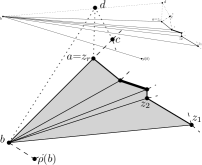
Figure 5: Illustration for the proof of Theorem. 2. The edge with slope $\alpha_{min}$ is thicker.

Consider the slopes $\alpha_{i}$ of the edges $(z_{i},z_{i+1})$ for $1\leq i<r$, and let $\alpha_{\min}$ be the negative slope with the least absolute value among them; see the bold edge in Figure 5. Let $s$ be the (negative) slope of the edge $(b,\rho(b))$. We aim at obtaining a drawing where $|s|\leq|\alpha_{\min}|$. To this aim, we apply the shift operation on $\rho(b)$ by $x$ units to the right, which stretches and flattens the edge $(b,\rho(b))$. If $|\alpha_{\min}|=h/w$, and $|s|=h^{\prime}/w^{\prime}$, then the value of $x$ is the first even integer such that $x\geq(h^{\prime}w-hw^{\prime})/h$. Now we have that $|s|=h^{\prime}/(w^{\prime}+x)\leq h^{\prime}/(w^{\prime}-h^{\prime}w/h-w^{\prime})=h/w=|\alpha_{\min}|$. The fact that $x$ is even preserves the even length of the edges on the contour. This preliminary operation will be useful in the following.

Next, let $\Delta(b)=y(b)-y(\rho(b))>0$ and let $\Delta(c)=y(c)-y(b)>0$ , i.e., $b$ lies $\Delta(b)$ rows above $\rho(b)$, and $c$ lies $\Delta(c)$ rows above $b$, where the edges $(b,a)$ and $(a,c)$ have slope $+1$. We apply the following procedure to lift $b$ at the same $y$-coordinate of $c$. (i) We undo the placement of all vertices in $\mathcal{A}_{l}(b)$. (ii) If $\Delta(c)$ is not a multiple of $\Delta(b)$, say $\Delta(b)+\delta=q\cdot\Delta(c)$ for some integer $q$, then we shift $\rho(c)$ by $2\delta$ units to the right. This implies that $c$ moves by $(\delta,\delta)$ above its former position. (iii) We set the $y$-coordinate of vertex $b$ equal to the $y$-coordinate of $c$. To that end, we stretch the edge $(\rho(b),b)$ by the factor $q$. Let $w^{\prime}$ be the width and $h^{\prime}$ be the height of the edge $(\rho(b),b)$. The new edge has the same slope as before, and has width $qw^{\prime}$ and height $qh^{\prime}$. This implies shifting all vertices $\rho(b),z_{1},\ldots,z_{r-1},a,c$ by $(q-1)w^{\prime}$ units to the right. Vertex $b$ may need a further adjustment by a single unit left shift if $b=\lambda(d)$ and the intersection point of the $\pm 1$ diagonals through $\lambda(d)$ and $\rho(d)$ is not a grid point. Also, we apply the shift operation on $\lambda(b)$ by $(q-1)h^{\prime}$ units to the left. This particular lifting operation applied on vertex $b$ preserves planarity, which could be violated only by edges incident to $b$. Namely, if vertex $w$ is a neighbor of $b$ in $\mathcal{U}(b)$, then the edge $(w,b)$ is vertically stretched by $(q-1)h^{\prime}$ units. This cannot enforce a crossing, since it means a vertical shift of $w$. Clearly, $b$ can see $\rho(b)$, since the edge was stretched. Consider the upper right neighbors $z_{1},\ldots,z_{r}$ with $z_{r}=a$ of $b$. The edges $(b,z_{i})$ change direction from right upward to right downward. Since the absolute value of the slope of the edge $(b,\rho(b))$ is bounded from above by $\alpha_{\min}$ and since $y(\rho(b))\leq y(b)\leq y(z_{i});1\leq i\leq r$, the new position of $b$ is below the line spanned by each edge $(z_{i},z_{i+1})$ for $1\leq i<r$. Hence, $b$ can see each such neighbor $z_{i}$, including $a=z_{r}$. The lifting of $b$ has affected all vertices $v\in\mathcal{A}_{l}(b)$ with $y(v)<y(d)$. (iv) We re-insert the vertices in $\mathcal{A}_{l}(b)$, by changing $\sigma$ accordingly, as already explained for Case 1.

Finally, we place $d=\operatorname{top}(K)$. First, we place $d$ at the intersection point of the $\pm 1$ diagonals through $\lambda(d)$ and $\rho(d)$. Then, we adjust $d$ such that it lies vertically above $a$. If the preliminary position of $d$ is $t$ units to the left (right) of $a$, then we apply the shift operation on $\rho(d)$ by $2t$ units to the right (on $\lambda(d)$ by $2t$ units to the left).

Case 3: $b\prec a$ and $c\prec a$. This implies that $b=\lambda(a)$ and $c=\rho(c)$. The edges $(b,a)$ and $(c,a)$ have slope $+1$ and $-1$, respectively, as they belong to $C_{k}$. We now aim at having both $b$ and $c$ at the $y$-coordinate $y(a)+1$. To this end, we use the procedure described in Case 2 to lift $b$ upwards by $y(a)+1-y(b)$ rows by using a dummy vertex $c^{\prime}$ at position $(x(c),y(a)+1)$ as a reference point. Note that this lifting only affects $b$ and the vertices in $\mathcal{A}_{l}(b)$ (all other vertices are moved uniformly), so both $a$ and $c$ remain at their position. Hence, we now have the situation $c\prec a\prec b$ and can again use the procedure of Case 2 to solve this case.

To conclude the proof, we need to consider the first edge of the construction which is drawn horizontal. Since the lift operation requires an edge that does not have slope 0, we may need to introduce dummy vertices and edges. Namely, if there is a kite including the base edge $(v_{1},v_{2})$, then we add two dummy vertices $1^{\prime},2^{\prime}$ below it that form a new base edge $(v_{1}^{\prime},v_{2}^{\prime})$. We add the additional edges $(v_{1}^{\prime},v_{1})$, $(v_{1}^{\prime},v_{2})$, $(v_{1}^{\prime},v_{n})$, $(v_{2}^{\prime},v_{2})$ and $(v_{2}^{\prime},v_{n})$ to make the graph maximal planar. These dummy vertices and edges will be removed once the last vertex $v_{n}$ is placed.

In terms of time complexity, $G^{+}$ can be computed in $O(n)$ time, by Lemma 1. Furthermore, each shift, move and the lift operation can be implemented in $O(n)$ time, hence the placement of a single vertex costs $O(n)$ time. However, in some cases (in particular, when we are placing the top vertex of a kite), we may need to undo the placement of a set of vertices and re-insert them afterwards. Since when we undo and reinsert a set of vertices we also update $\sigma$ accordingly, this guarantees that the placement of the same set of vertices will not be undone anymore. Thus, the reinsertion of a set of $O(n)$ vertices costs $O(n^{2})$. Hence, we have $\sum^{n}_{i=1}O(n+n^{2})$ which gives an $O(n^{3})$ time complexity. ∎

Figure 6 shows a running example of our algorithm. Theorem 2 and the fact that there exist $n$-vertex RAC graphs with $4n-10$ edges [21] while an $n$-vertex IC-planar graph has at most $13n/4-6$ edges [54] imply that IC-planar graphs are a proper subfamily of RAC graphs.

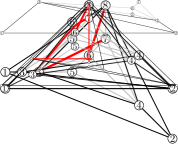
Figure 6: Example run of our algorithm on an IC-planar graph $G$ with a separating triangle. The crossing edges are drawn bold, the edges inside the separating triangle are drawn gray. (a) Input graph $G$. (b) Output of dFPP after vertex 7. (c) Output of dFPP after vertex 8. (d) Lifting 3 to the level of 7. (e) Moving 8 directly above 6.

We now show that exponential area is required for RAC drawings of IC-planar graphs. Since the vertices are not drawn on the integer grid, the drawing area is measured as the proportion between the longest and the shortest edge.

Theorem 3.

For every integer $k\geq 1$, there exists an IC-plane graph $G_{k}$ with $n_{k}$ vertices such that every IC-planar straight-line RAC drawing of $G_{k}$ takes area $\Omega(q^{n_{k}})$, for some constant $q>1$.

Proof.

Refer to Figures 7(a) and 7(b) for the construction of $G_{k}$, for $k\geq 1$. Each graph $G_{i}$, for $1\leq i\leq k$, has a 4-cycle as outer face, while all other faces are triangles (a triangle is composed of either three vertices or of two vertices and one crossing point). Two non-adjacent edges of the outer face are called the marked edges of $G_{i}$.

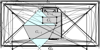
(a) The first three levels of the construction.

(b) Going from level $i-1$ to level $i$.

Figure 7: Illustration for the proof of Theorem 3.

Graph $G_{1}$ has 8 vertices, 4 inner vertices forming a kite, and 4 vertices on the outer face. All inner faces are triangles. The two marked edges of the outer face of $G_{1}$ are any two non-adjacent edges of this face. Graph $G_{i}$ is constructed from $G_{i-1}$ as follows, see also Figure 7(b). Let $\{A,B,C,D\}$ be the four vertices of the outer face of $G_{i-1}$, and let $(A,D)$ and $(B,C)$ be the two marked edges of $G_{i-1}$ (bold in Figure 7(b)). We attach a kite $(A,D,a,d)$ on the marked edge $(A,D)$ and a kite $(B,C,b,c)$ on the marked edge $(B,C)$. We connect the two kites with the edges $(a,B)$, $(a,b)$, $(c,D)$, and $(c,d)$. We then add a cycle between four further vertices $\{\alpha,\beta,\gamma,\delta\}$ that form the outer face of $G_{i}$, and we triangulate the inner face between the cycles $(\alpha,\beta,\gamma,\delta)$ and $(a,b,c,d)$. We set the edges $(\alpha,\beta)$ and $(\gamma,\delta)$ as the marked edges of $G_{i}$.

An embedding-preserving straight-line RAC drawing $\Gamma_{k}$ of $G_{k}$ ($k\geq 1$) with minimum area can be obtained by drawing each kite as a quadrilateral, as shown in Figures 7(a) and 7(b). Since vertex $a$ is connected to vertex $B$, $a$ has to lie above the line spanned by the edge $(A,B)$. Further, since vertex $d$ is connected to vertex $C$, $d$ has to lie below the line spanned by the edge $(C,D)$. This implies that the quadrilateral $(A,D,a,d)$ contains the square that has the edge $(A,D)$ as its right side. Hence, the width increases by at least the length of edge $(A,D)$. Note that one might extend the edge $(B,C)$ to make $(A,D,a,d)$ smaller. However, since we also have the edges $(a,b)$ and $(c,d)$, this procedure increases the size of $(B,C,b,c)$ such that, as soon as $(a,d)$ is smaller than $(A,D)$, it has to be that $(b,c)$ is larger than $(B,C)$ (to keep the visibility required for $(a,b)$ and $(c,d)$). Then, this implies that the quadrilateral $(B,C,b,c)$ contains the square that has the edge $(B,C)$ as its left side, so the width increases by at least the length of edge $(B,C)$.

The minimum-area drawing forces the outer face of every subgraph $G_{i}$ ($i\leq k$) of $G_{k}$ to be a rectangle $R_{i}$. We denote by $l_{i}$ ($L_{i}$) the length of the shortest (longest) side of $R_{i}$. The area of $R_{i}$ is $A_{i}=l_{i}\times L_{i}$. Observe that, by construction, the marked edges of $G_{i}$ have length $L_{i}$. It follows that $l_{i}\geq L_{i-1}+4$ and $L_{i}\geq l_{i-1}+L_{i-1}+2$. Therefore, $A_{i}\geq(L_{i-1}+4)\times(l_{i-1}+L_{i-1}+2)\geq A_{i-1}+A_{i-1}=2A_{i-1}$, hence $A_{k}\geq 2A_{k-1}\geq 2^{k-1}A_{1}\geq 2^{k+1}$. The number of vertices of $G_{k}$ is $n_{k}=8k$, and hence $k=\frac{n_{k}}{8}$. Thus $A_{k}\geq 2^{\frac{n_{k}}{8}}\geq 1.09^{n_{k}}$, which proves the statement. ∎

5 Recognizing IC-planar graphs

The IC-planarity testing problem asks if a graph $G$ admits an IC-planar embedding.

Hardness of the problem. The next theorem shows that IC-planarity testing is $\mathrm{NP}$-complete.

Theorem 4.

IC-planarity testing is $\mathrm{NP}$-complete.

(a) $G$

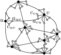
(b) $G^{*}$

Figure 8: Illustration of the proof of Theorem 4.

Proof.

IC-planarity is in $\mathrm{NP}$, as one can guess an embedding and check whether it is IC-planar [29]. For the hardness proof, the reduction is from the 1-planarity testing problem, which asks whether a given graph is 1-planar or not. The reduction uses a $3$-cycle gadget and exploits the fact that at most one edge of a $3$-cycle is crossed in an IC-planar drawing. We transform an instance $G$ of 1-planarity testing into an instance $G^{*}$ of IC-planarity testing, by replacing each edge $(u,v)$ of $G$ with a graph $G_{uv}$ consisting of two $3$-cycles, $T_{uv}$ and $T_{vu}$, with vertices $\{u,c_{uv},a_{uv}\}$ and $\{v,c_{vu},a_{vu}\}$, respectively, plus edge $(a_{uv},a_{vu})$, called the attaching edge of $u$ and $v$; see Figure 8.

Let $\Gamma$ be a 1-planar drawing of $G$. An IC-planar drawing $\Gamma^{*}$ of $G^{*}$ can be easily constructed by replacing each curve representing an edge $(u,v)$ in $\Gamma$ with a drawing of $G_{uv}$ where $T_{uv}$ and $T_{vu}$ are drawn planar and sufficiently small, such that the possible crossing that occurs on the edge $(u,v)$ in $\Gamma$ occurs on the attaching edge $(a_{uv},a_{vu})$ in $\Gamma^{*}$. Hence, since all the attaching edges are independent, $\Gamma^{*}$ is IC-planar.

Let $\Gamma^{*}$ be an IC-planar drawing of $G^{*}$. We show that it is possible to transform the drawing in such a way that all crossings occur only between attaching edges. Once this condition is satisfied, in order to construct a 1-planar drawing $\Gamma$ of $G$, it suffices to remove, for each edge $(u,v)$, the vertices $c_{uv}$ and $c_{vu}$, and to replace $a_{uv}$ and $a_{vu}$ with a bend point. Namely, as already observed, no more than one edge can be crossed for every gadget $T_{uv}$ of $G^{*}$. Suppose now that the edge $(u,a_{uv})$ of $T_{uv}$ is crossed. Since the other two edges of $T_{uv}$ are not crossed, we can reroute $(u,a_{uv})$ such that it follows the curves that represent $(u,c_{uv})$ and $(c_{uv},a_{uv}$); see Figure 9.

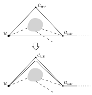
Figure 9: Illustration of the proof of Theorem 4. (a) Rerouting the crossed edge $(u,a_{uv})$ via $c_{uv}$ to be planar. (b) Rerouting the crossing edges $(u,v)$ and $(u,w)$ to be planar.

In order to complete the proof, we need to take care of the following particular case. Two attaching edges $a_{uv}$ and $a_{uw}$ that cross and that are connected to two gadgets $T_{uv}$ and $T_{uw}$ with a common vertex $u$ represent a valid configuration in $\Gamma^{*}$, while they give rise to a crossing between two adjacent edges in $\Gamma$, which is not allowed since $\Gamma$ must be a simple drawing. However, this case can be easily solved, since the two edges do not cross any others, by rerouting them in $\Gamma$ as shown in Figure 9. ∎

Note that this construction does not work for IC-planarity testing with a given rotation system since the rerouting step changes the rotation system. However, we now prove $\mathrm{NP}$-hardness of IC-planarity testing for graphs with a given rotation system. We rely on the membrane technique introduced by Auer et al. [7] to prove the $\mathrm{NP}$-hardness of 1-planarity testing for graphs with a given rotation system. In particular, we design gadgets that make it possible to use the membrane technique in the case of IC-planar graphs.

First, we replace the U-graphs [7] by M-graphs, called mesh graphs. These graphs have a unique embedding with a fixed rotation system. Namely, an M-graph is a mesh, where cells are filled with two crossing edges, following a checkerboard pattern to ensure independent crossings; see Figure 10. To see that with a given rotation system, an M-graph has a unique embedding, observe that each subgraph isomorphic to $K_{4}$ can be embedded planarly or as a kite, and this is determined by the rotation system [41]. The rotation system defined by the drawing in Figure 10 implies that each subgraph isomorphic to $K_{4}$ is embedded as a kite, and therefore the embedding of an M-graph is unique.

Let $M$ be an M-graph with a given fixed embedding. At its bottom line, $M$ has sufficiently many free vertices that are not incident with a crossing edge in $M$. These vertices are consecutively ordered, say from left to right. The edges on the bottom line are not crossed in any IC-planar embedding of $M$, so they are crossing-free in the given embedding. Finally, $M$ cannot be crossed by any path from a free vertex. In what follows, we attach further gadgets to $M$ by connecting these gadgets to consecutive free vertices. If there are several gadgets, then they are separated and placed next to each other.

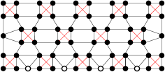
Figure 10: The structure of an M-graph (a) and its abbreviation (b).

General Construction

Consider an instance $\alpha$ of planar-3SAT with its corresponding plane graph $G$ and its dual $G^{*}$. Recall that the vertices of $G$ represent variables $x$ and clauses $c$, also, there is an edge $(x,c)$ if $x$ or its negation occurs as a literal in $c$; see Figure 11. We transform $G^{*}$ into an M-supergraph $G^{*}_{\alpha}$ (see Figure 11) as follows.

Each vertex of $G^{*}$, corresponding to a face of the embedded graph $G$, is replaced by a sufficiently large M-graph. Further, each edge of $G^{*}$ is replaced by a barrier of $l$ parallel edges between $l$ consecutive free vertices on the boundaries of the two M-graphs of the adjacent faces. These edges will be crossed by paths that are called ropes. The size of $l$ will be determined later.

For each variable $x$, we construct a V-gadget $\gamma(x)$, and similarly we build a C-gadget for each clause. These gadgets are described below.

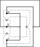
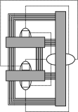
Figure 11: (a) The planar graph $G$ (solid) and its dual $G^{*}$ (dotted) corresponding to the planar-3SAT formula $(a\vee b\vee\neg c)\wedge(a\vee\neg b\vee c)$. (b) The corresponding M-supergraph $G^{*}_{\alpha}$ with the clause gadgets (vertical) and the variable gadgets (horizontal).

Each vertex $u$ of $G$ lies on the boundary of a face $f$ of $G$. We attach the gadget $\gamma(u)$ of $u$ to the M-graph at $f$ so that $\gamma(u)$ lies in $f$. It does not matter which face $f$ incident to $u$ is chosen. Similarly, each edge $e$ of $G$ between a variable and a clause is replaced by a rope of length $2l+3$. Since $e$ is crossed by its dual edge, the rope is crossed by a barrier. A rope acts as a communication line that “passes” a crossing at a V-gadget across a barrier to a C-gadget. We denote by a membrane (similarly as in [7]) a path between free vertices on the boundary of a single M-graph, or between particular vertices of a variable gadget. We call a vertex IN if it is placed inside the region of a membrane and the boundary of the M-graph in an IC-drawing, and OUT otherwise. IN and OUT are exactly defined by edges which cross the membrane. Note that the framework is basically a simultaneous embedding of $G$ and $G^{*}$ by means of our gadgets, M-graphs, barriers and ropes. The subgraph without V- and C-gadgets is 3-connected, since the M-graphs are 3-connected and the barriers have size $l$ for $l\geq 3$, and it has a unique planar embedding if one edge from each pair of crossing edges in each M-graph is removed.

Construction of the C-gadgets

The C-gadget $c=(l_{1},l_{2},l_{3})$ with three literals $l_{1}$, $l_{2}$ and $l_{3}$ is attached to eight consecutive free boundary vertices of an M-graph $M$, say $v_{1},\ldots,v_{8}$. For each literal $l_{i}$, there are three vertices $u_{i}$, $a_{i}$ and $b_{i}$, and four edges $(u_{i},a_{i})$, $(u_{i},b_{i})$, $(a_{i},v_{2i})$ and $(b_{i},v_{2i+1})$, where $u_{i}$ is the initial vertex of the rope towards the corresponding variable gadget. There is a membrane of nine edges from $v_{1}$ to $v_{8}$, see Figure 12.

By construction, at most two vertices among $u_{1}$, $u_{2}$ and $u_{3}$ can be moved outside the membrane, and at least one initial vertex of a rope (and maybe all) must be IN. IN shall correspond to the value true of the literal and thus of the clause.

Construction of the V-gadgets

Let $x$ be a variable and let $v$ be the vertex corresponding to $x$ in $G$. Suppose that the literal $x$ occurs in $k$ clauses for some $k\geq 1$, which are ordered by the embedding of $G$. Denote this sequence by $x_{1},\ldots x_{k}$, where each $x_{i}$ corresponds to $x$ or $\neg x$. The V-gadget of $x$ is $\gamma(x)=\gamma(x_{0}),\gamma(x_{1}),\ldots,\gamma(x_{k}),\gamma(x_{k+1})$. This gadget is connected to $7(k+2)$ free consecutive vertices on the border of the M-graph $M$ to which it is attached; see Figure 12 for an illustration. The gadgets $\gamma(x_{0})$ and $\gamma(x_{k+1})$ are called the (left and right) terminal gadgets and each $\gamma(x_{i})$ ($1\leq i\leq k$) is called a literal gadget. Gadget $\gamma_{i}$ for $0\leq i\leq k+1$ is similar to a clause gadget and is connected to seven consecutive free variables $v^{i}_{1},\ldots,v^{i}_{7}$ on the boundary of $M$. There is a local membrane of seven edges from $v^{i}_{1}$ to $v^{i}_{7}$.

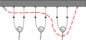
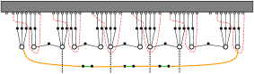
Figure 12: (a) The clause gadget. (b) The variable gadget.

The left terminal gadget $\gamma(x_{0})$ has two primary vertices $x_{0}^{+}$ and $x_{0}^{-}$. The primary vertex $x_{0}^{+}$ is connected to $v^{0}_{2}$, $v^{0}_{3}$ and $v^{0}_{4}$ by paths of length two. The other primary vertex $x_{0}^{-}$ is connected to $v^{0}_{5},v^{0}_{6}$ also by paths of length two. Analogously, the right terminal gadget has two primary vertices $x_{k+1}^{+}$ and $x_{k+1}^{-}$, with the same requirements. The gadget $\gamma(x)$ has an outer membrane of length $2k+1$ from $x_{0}^{+}$ to $x_{k+1}^{-}$.

Each literal gadget $\gamma(x_{i})$ has has two primary vertices $x_{i}^{+}$ and $x_{i}^{-}$. If $x_{i}$ is positive, then $x_{i}^{+}$ is attached to three free vertices $v^{i}_{2}$, $v^{i}_{3}$ and $v^{i}_{4}$ of $M$, and $x_{i}^{-}$ is attached to two free vertices $v^{i}_{5}$ and $v^{i}_{6}$ by two paths of length two, respectively. The rope to the literal begins at $x_{i}^{+}$. Otherwise, if $x_{i}$ is negated, then the gadget is reflected, such that $x_{i}^{+}$ has two, and $x_{i}^{-}$ has three paths of length two to the M-graph. The rope to the literal begins at $x_{i}^{-}$. The rope is a path of $2l+3$ edges from vertex $x_{i}^{\pm}$ of the V-gadget to the vertex $u_{j}$ of the clause gadget representing the literal of $x$. In addition, there is a path of length two that connects $x_{i}^{-}$ to $x_{i+1}^{-}$ for all $0\leq i\leq k$.

The M-graph must have sufficiently many free vertices for the edges from the gadgets and barriers. The smallest bound can easily be computed from the embedding of $G$ and the attached gadgets; see Figure 11. The rotation system of the gadgets is retrieved from the drawing and the ordering of the vertices on the border of M-graphs.

Correctness

We will now prove several lemmas on the structure of our construction. With these lemmas, we will show that an IC-planar drawing of the resulting graph $G_{\alpha}$ immediately yields a valid solution to the underlying planar-3SAT problem. First, we show that the M-graph is not crossed.

Lemma 2.

The boundary edges of an M-graph (with a fixed rotation system) are never crossed in an IC-planar drawing of $G_{\alpha}$.

Proof.

This lemma follows directly from the construction. Each $K_{4}$ must be embedded as a kite, and further edge crossings violate IC-planarity. ∎

Consequently, the following corollary holds.

Corollary 1.

A path from a free boundary vertex cannot cross any M-graph.

Now, we show that every clause, terminal and literal gadget has at least one primary vertex that is not OUT.

Lemma 3.

In every IC-planar drawing of $G_{\alpha}$, at most two of the primary vertices $u_{1}$, $u_{2}$ and $u_{3}$ of a clause gadget can be OUT, and at most one of the primary vertices $x_{i}^{+},x_{i}^{-}$ of a terminal or a literal gadget can be OUT of the local membrane.

Proof.

Assume that $u_{1}$, $u_{2}$ and $u_{3}$ all are OUT. Then, the membrane must cross five edges. Since the membrane has length seven, either one membrane edge is crossed twice or two adjacent membrane edges are crossed, which contradicts the IC-planarity of the drawing. The proof for terminal and literal gadgets works analogously. ∎

Next, we show that the outer membrane crosses each rope.

Lemma 4.

In every IC-planar drawing of $G_{\alpha}$, each rope connected to a V-gadget is crossed by the outer membrane of the V-gadget.

Proof.

Suppose some rope is not crossed by the outer membrane. Either the outer membrane crosses at least one barrier or it crosses the three paths of length two that connect the V-gadget endpoint of the rope to its M-graph. It cannot do the first if the size of the barrier is chosen to be

$$l\geq\max\{k\mid\text{a variable }x\text{ occurs in }k\text{ clauses of }\alpha\}+2.$$

It cannot do the second since the outer membrane, of length $2k+1$, would be crossed at least $k+2$ times. ∎

The fact that a rope propagates a truth value is due to the fact that its length is tight, as the following lemma shows.

Lemma 5.

In every IC-planar drawing of $G_{\alpha}$, respecting the rotation system, the endpoint of a rope at a C-gadget is OUT if the endpoint at the vertex is IN (its local membrane).

Proof.

M-graphs, by construction, cannot be crossed by a rope. Thus, the rope must cross a barrier of $l$ edges. In addition, a rope is crossed by the outer membrane of the variable gadget. If the endpoint at the vertex is IN (its local membrane), then the rope is crossed by $l+2$ edges. Hence, it cannot cross another membrane, since its length is $2l+3$. ∎

The consistency of the truth assignment of the variable is granted by the following lemma.

Lemma 6.

In every IC-planar drawing of $G_{\alpha}$, and every variable $x$, either $x_{i}^{+}$ is OUT (and $x_{i}^{-}$ is IN) for all $0\leq i\leq k+1$ or $x_{i}^{+}$ is IN (and $x_{i}^{-}$ is OUT) for all $0\leq i\leq k+1$.

Proof.

If $x_{0}^{+}$ is OUT, then by Lemma 3 $x_{0}^{-}$ is IN and the local membrane must cross an edge of the path of length two from $x_{0}^{+}$ to $x_{1}^{-}$. This implies that the local membrane of the first literal gadget cannot cross this path, and therefore must cross the paths from $x_{1}^{+}$ to the M-graph. It follows by induction that all $x_{i}^{+}$ are OUT and all $x_{i}^{-}$ are IN; see Figure 12. If $x_{0}^{+}$ is IN, then the outer membrane insures that $x_{k+1}^{-}$ is OUT. We then proceed from right to left. Now, all $x_{i}^{-}$ are OUT and all $x_{i}^{+}$ are IN. ∎

With these lemmas, we can finally prove the following theorem.

Theorem 5.

IC-planarity testing with given rotation system is $\mathrm{NP}$-complete.

Proof.

We have already stated in the proof of Theorem 4 that IC-planarity is in $\mathrm{NP}$. We reduce from planar-3SAT and show that an expression $\alpha$ is satisfiable if and only if the constructed graph $G^{*}_{\alpha}$ has a IC-planar drawing. If $\alpha$ is satisfiable, then we draw the V- and C-gadgets according to the assignment, such that the initial vertex of each rope from the gadget of a variable $x$ is IN at the C-gadget if the literal is assigned the value true. The resulting drawing is IC-planar by construction. If $G^{*}_{\alpha}$ has an IC-planar drawing, then we obtain the truth assignment of $\alpha$ from the drawing. Thus, IC-planarity with a given rotation system is $\mathrm{NP}$-complete. ∎

Note that the construction for the proof of Theorem. 5 also holds in the variable embedding setting, since the used graphs have an almost fixed IC-planar embedding. From this, we can obtain an alternative $\mathrm{NP}$-completeness proof of IC-planarity testing.

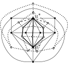
Figure 13: (a) A triconnected graph $T$ (solid) and its dual $T^{*}$ (dotted), (b) The extended graph $T^{*}\cup\{u^{*},v^{*}\}$ and the three length-3 paths between $u^{*}$ and $v^{*}$ (bold). (c) The ordered routing edges $e_{1},\ldots,e_{k}$ lie inside the quadrangle $(u,l_{uv},v,r_{uv})$.

5.1 Polynomial-time test for a triangulated plane graph plus a matching

On the positive side, we now describe an $O(n^{3})$-time algorithm to test whether a graph $G=(V,E_{T}\cup E_{M})$ that consists of a triangulated plane graph $T=(V,E_{T})$ and a matching $M=(V_{M},E_{M})$ with $V_{M}\subseteq V,E_{M}\cap E_{T}=\emptyset$ admits an IC-planar drawing that preserves the embedding of $T$. In the positive case the algorithm also computes an IC-planar drawing. An outline of the algorithm is as follows. (1) Check for every matching edge if there is a way to draw it such that it crosses only one edge of $T$. (2) Split $T$ into subgraphs that form a hierarchical tree structure. (3) Traverse the 4-block tree bottom-up and solve a 2SAT formula for each tree node.

In order to check whether there is a valid placement for each matching edge $(u,v)\in M$, we have to find two adjacent faces, one of which is incident to $u$, while the other one is incident to $v$. To this end, we consider the dual $T^{*}$ of $T$ that contains a vertex for each face in $T$ that is not incident to a vertex $w\in V_{M}\setminus\{u,v\}$, and an edge for each edge in $T$ that separates two faces. Further, we add two additional vertices $u^{*}$ and $v^{*}$ to $T^{*}$ that are connected to all faces that are incident to $u$ and $v$, respectively. In the resulting graph $T^{*}\cup\{u^{*},v^{*}\}$, we look for all paths of length 3 from $u^{*}$ to $v^{*}$. These paths are equivalent to routing $(u,v)$ through two faces that are separated by a single edge. Note that no path of length 1 or 2 can exist, since $(i)$ by construction $u^{*}$ and $v^{*}$ are not connected by an edge and $(ii)$ if there was a path of length 2 between $u^{*}$ and $v^{*}$, then $u$ and $v$ would lie on a common face in the triangulated graph $T$; thus, the edge $(u,v)$ would exist both in $E_{T}$ and in $E_{M}$, which is not possible since $E_{T}\cap E_{M}=\emptyset$. See Figure 13 for an illustration. If there is an edge that has no valid placement, then $G$ is not IC-planar and the algorithm stops. Otherwise, we save each path that we found as a possible routing for the corresponding edge in $M$.

Now, we make some observations on the structure of the possible routings of an edge $(u,v)\in M$ that we can use to get a hierarchical tree structure of the graph $T$. Every routing is uniquely represented by an edge that separates a face incident to $u$ and a face incident to $v$ and that might be crossed by $(u,v)$. We call these edges routing edges. Let there be $k$ routing edges for the pair $(u,v)$. Each of these edges forms a triangular face with $u$. From the embedding, we can enumerate the edges by the counterclockwise order of their corresponding faces at $u$. This gives an ordering $e_{1},\ldots,e_{k}$ of the routing edges. Let $e_{1}=(l_{uv},l^{\prime}_{uv})$ and $e_{k}=(r^{\prime}_{uv},r_{uv})$ such that the edge $(u,l_{uv})$ comes before the edge $(u,l^{\prime}_{uv})$, and the edge $(u,r^{\prime}_{uv})$ comes before $(u,r_{uv})$ in the counterclockwise order at $u$. Then, all edges $e_{1},\ldots,e_{k}$ lie within the routing quadrangle $(u,l_{uv},v,r_{uv})$; see Figure 13. Note that there may be more complicated structures between the edges, but they do not interfere with the ordering. Denote by $Q_{uv}=(u,l_{uv},v,r_{uv})$ the routing quadrilateral of the matching edge $(u,v)\in M$. We define the interior $\mathcal{I}_{uv}=(\mathcal{V}_{uv},\mathcal{E}_{uv})$ as the maximal subgraph of $T$ such that, for every vertex $w\in\mathcal{V}_{uv}$, each path from $w$ to a vertex on the outer face of $T$ contains $u$, $l_{uv}$, $v$, or $r_{uv}$. Consequently, $Q_{uv}\in\mathcal{V}_{uv}$. We will now show that two interiors cannot overlap.

Lemma 7.

For each pair of interiors $\mathcal{I}_{uv},\mathcal{I}_{ab}$, exactly one of the following conditions holds: (a) $\mathcal{I}_{uv}\cap\mathcal{I}_{ab}=\emptyset$ (b) $\mathcal{I}_{uv}\subset\mathcal{I}_{ab}$ (c) $\mathcal{I}_{ab}\subset\mathcal{I}_{uv}$ (d) $\mathcal{I}_{uv}\cap\mathcal{I}_{ab}=Q_{uv}\cap Q_{ab}$.

Proof.

Assume that neither of the conditions holds. Recall that $Q_{uv}$ and $Q_{ab}$ are the boundaries of the interiors. Note that $\mathcal{I}_{uv}\cap\mathcal{I}_{ab}=\emptyset$ corresponds to disjointness, $\mathcal{I}_{uv}\subset\mathcal{I}_{ab}$ and $\mathcal{I}_{ab}\subset\mathcal{I}_{uv}$ correspond to inclusion, and $\mathcal{I}_{uv}\cap\mathcal{I}_{ab}=Q_{uv}\cap Q_{ab}$ corresponds to touching in their boundary of the two interiors $\mathcal{I}_{uv}$ and $\mathcal{I}_{ab}$. Thus, if the conditions do not hold, the interiors must properly intersect, that is, without loss of generality, there is a vertex $c\in Q_{uv}$ that lies in $\mathcal{I}_{ab}\setminus Q_{ab}$, and a vertex $d\in Q_{uv}$ that does not lie in $\mathcal{I}_{ab}$. Hence, the other two vertices of $Q_{uv}$ lie in $Q_{ab}$. Clearly, $c$ and $d$ are opposite vertices in $Q_{uv}$. By definition of IC-planar graphs, it holds that $\{a,b\}\cap\{u,v\}=\emptyset$.

First, assume that $c=l_{uv}$. Then, $u$ and $v$ must lie in $Q_{ab}$. More specifically, by definition of IC-planar graphs $\{u,v\}=\{l_{ab},r_{ab}\}$. Without loss of generality, assume that $u=r_{ab}$ and $v=l_{ab}$. Since the edges $(u,c)$ and $(v,c)$ have to lie in $\mathcal{I}_{ab}$, this leads to the situation depicted in Figure 14. However, this implies that that there are only two routing edges for $(a,b)$ with one of them incident to $u$, and the other one is incident to $v$. Thus, the routing edges are not valid. The case that $c=r_{uv}$ works analogously.

Second, assume that $c=u$. Then, $l_{uv}$ and $r_{uv}$ must lie in $Q_{ab}$. If $l_{uv}$ and $r_{uv}$ are adjacent on $Q_{ab}$, say $l_{uv}=b$ and $r_{uv}=r_{ab}$, then there is only a single routing edge for $(u,v)$ that is incident to $b$ and thus not valid; see Figure 14. Otherwise, there are two cases. If $\{l_{uv},r_{uv}\}=\{a,b\}$, say $r_{uv}=a$ and $l_{uv}=b$, then there are only two routing edges for $(u,v)$ with one of them incident to $a$, and the other one incident to $b$; see Figure 14. If $\{l_{uv},r_{uv}\}=\{l_{ab},r_{ab}\}$, say $l_{uv}=l_{ab}$ and $r_{uv}=r_{ab}$, then both routing edges of $(u,v)$ are incident to $b$; see Figure 14. The case that $c=v$ works analogously.

This proves that, if there is a proper intersection between two routing quadrilaterals, than at least one of the corresponding matching edges has no valid routing edge. Thus, one of the conditions must hold. ∎

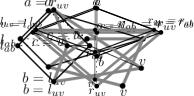
Figure 14: Illustration of the proof of Lemma 7. The routing quadrilateral $Q_{ab}$ is drawn bold, and $Q_{uv}$ is drawn dark gray and thicker. (a) $l_{uv}$ lies in $\mathcal{I}_{ab}\setminus Q_{ab}$. (b) $l_{uv}$ and $r_{uv}$ are adjacent in $Q_{ab}$. (c) $\{l_{uv},r_{uv}\}=\{a,b\}$. (d) $\{l_{uv},r_{uv}\}=\{l_{ab},r_{ab}\}$.

By using Lemma 7, we can find a hierarchical structure on the routing quadrilaterals. We construct a directed graph $H=(V_{H},E_{H})$ with $V_{H}=\{\mathcal{I}_{uv}\mid(u,v)\in M\}\cup\{G\}$. For each pair $\mathcal{I}_{uv},\mathcal{I}_{xy}$, $E_{H}$ contains a directed edge $(\mathcal{I}_{uv},\mathcal{I}_{xy})$ if and only if $\mathcal{V}_{uv}\subset\mathcal{V}_{xy}$ and there is no matching edge $(a,b)$ with $\mathcal{V}_{uv}\subset\mathcal{V}_{ab}\subset\mathcal{V}_{xy}$. Finally, we add an edge from each subgraph that has no outgoing edges to $G$. Each vertex but $G$ only has one outgoing edge. Obviously, this graph contains no (undirected) cycles. Thus, $H$ is a tree.

We will now show how to construct a drawing of $G$ based on $H$ in a bottom-up fashion. We will first look at the leaves of the graph. Let $\mathcal{I}_{uv}$ be a vertex of $H$ whose children are all leaves. Let $\mathcal{I}_{u_{i}v_{i}},\ldots,\mathcal{I}_{u_{k}v_{k}}$ be these leaves. Since these interiors are all leaves in $H$, we can pick any of their routing edges. However, the interiors may touch on their boundary, so not every combination of routing edges can be used. Assume that a matching edge $(u_{i},v_{i}),1\leq i\leq k$ has more than two valid routing edges. Then, we can always pick a middle one, that is, a routing edge that is not incident to $l_{u_{i}v_{i}}$ and $r_{u_{i}v_{i}}$, since this edge will not interfere with a routing edge of another matching edge.

Now, we can create a 2SAT formula to check whether there is a valid combination of routing edges as follows. For the sake of clarity, we will create several redundant variables and formulas. These can easily be removed or substituted by shorter structures to improve the running time. For each matching edge $(u_{i},v_{i}),1\leq i\leq k$, we create two binary variables $l_{i}$ and $r_{i}$, such that $l_{i}$ is true if and only if the routing edge incident to $l_{u_{i}v_{i}}$ is picked, and $r_{i}$ is true if and only if the routing edge incident to $r_{u_{i}v_{i}}$ is picked. If $(u_{i},v_{i})$ has only one routing edge, then it is obviously incident to $l_{u_{i}v_{i}}$ and $r_{u_{i}v_{i}}$, so we set $l_{u_{i}v_{i}}=r_{u_{i}v_{i}}=\texttt{true}$ by adding the clauses $l_{u_{i}v_{i}}\vee\texttt{false}$ and $r_{u_{i}v_{i}}\vee\texttt{false}$. If $(u_{i},v_{i})$ has exactly two routing edges, the picked routing edge has to be incident to either $l_{u_{i}v_{i}}$ or $r_{u_{i}v_{i}}$, so we add the clauses $l_{u_{i}v_{i}}\vee r_{u_{i}v_{i}}$ and $\neg l_{u_{i}v_{i}}\vee\neg r_{u_{i}v_{i}}$. If $(u_{i},v_{i})$ has more than two routing edges, we can pick a middle one, so we set $l_{u_{i}v_{i}}=r_{u_{i}v_{i}}=\texttt{false}$ by adding the clauses $\neg l_{u_{i}v_{i}}\vee\texttt{false}$ and $\neg r_{u_{i}v_{i}}\vee\texttt{false}$. Next, we have to add clauses to forbid pairs of routing edges that can not be picked simultaneously, i.e., they share a common vertex. Consider a pair of matching edges $(u_{i},v_{i}),(u_{j},v_{j}),1\leq i,j\leq k$. If $r_{u_{i}v_{i}}$=$l_{u_{j}v_{j}}$, we add the clause $\neg r_{i}\vee\neg l_{j}$. For the other three cases, we add an analogue clause.

Now, we use this 2SAT to decide whether the subgraph $I_{uv}$ is IC-planar, and which routing edges can be used. For each routing edge $(a,b)$ of $I_{uv}$, we solve the 2SAT formula given above with additional constraints that forbid the use of routing edges incident to $a$ and $b$. To that end, add the following additional clauses: If $l_{u_{i}v_{i}}=a$, add the clause $\neg l_{i}\vee\texttt{false}$. For the other three cases, we add an analogue clause. If this 2SAT formula has no solution, then the subgraph $\mathcal{I}_{uv}$ is not IC-planar. Otherwise, there is a solution where you pick the routing edges corresponding to the binary variables. To decide whether a subgraph $I_{uv}$ whose children are not all leaves is IC-planar, we first compute which of their routing edges can be picked by recursively using the 2SAT formula above. Then, we use the 2SAT formula for $I_{uv}$ to determine the valid routing edges of $I_{uv}$. Finally, we can decide whether $G$ is IC-planar and, if yes, get a drawing by solving the 2SAT formula of all children of $G$.

Hence, we give the following for the proof of the time complexity.

Theorem 6.

Let $T=(V,E_{T})$ be a triangulated plane graph with $n$ vertices and let $M=(V,E_{M})$ be a matching. There exists an $O(n^{3})$-time algorithm to test if $G=(V,E_{T}\cup E_{M})$ admits an IC-planar drawing that preserves the embedding of $T$. If the test is positive, the algorithm computes a feasible drawing.

Proof.

We need to prove that the described algorithm runs in $O(n^{3})$ time. Indeed, for each subgraph $I_{uv}$, we have to run a 2SAT formula for each routing edge. Once we have determined the valid routing edges, we do not have to look at the children anymore. Let $c_{uv}$ be the number of children of $I_{uv}$. Each of these 2SAT formula contains $2c_{uv}$ variables and up to $4c_{uv}(c_{uv}-1)$ clauses. Since every edge of $G$ can only be a routing edge for exactly one matching edge, we have to solve at most $n$ 2SAT formulas. The tree $H$ consists of at most $n/2+1$ vertices (one for each matching edge), so a very conservative estimation is that we have to solve $O(n)$ 2SAT formulas with $O(n)$ variables and $O(n^{2})$ clauses each. Aspvall et al. [6] showed how to solve 2SAT in time linear in the number of clauses. We can use the linear-time algorithm of Section 3 to draw the IC-planar graph corresponding to the IC-planar embedding by picking the routing edges corresponding to the binary variables. Thus, our algorithm runs in $O(n^{3})$ time. ∎

6 Open Problems

The research presented in this paper suggests interesting open problems.

Problem 1.

We have shown that every IC-planar graph has a straight-line drawing in quadratic area, although the angle formed by any two crossing edges can be small. Conversely, straight-line RAC drawings of IC-planar graphs may require exponential area. From an application perspective, it is interesting to design algorithms that compute a straight-line drawing of IC-planar graphs in polynomial area and good crossing resolution.

Problem 2.

Also, although IC-planar graphs are both 1-planar and straight-line RAC drawable graphs, a characterization of the intersection between these two classes is still missing. In particular, studying whether NIC-planar graphs (see Zhang [53]), which lie between IC-planar graphs and 1-planar graphs, are also RAC graphs may lead to new insights on this problem.

Problem 3.

We proved that recognizing IC-planar graphs is NP-hard. Is it possible to design fixed-parameter tractable (FPT) algorithms for this problem, which improve the time complexity of those described by Bannister et al. [8] for 1-planar graphs, with respect to different parameters (vertex cover number, tree-depth, cyclomatic number)? Are there other parameters that can be conveniently exploited for designing FPT testing algorithms for IC-planar graphs?

References

- [1] E. Ackerman and G. Tardos. On the maximum number of edges in quasi-planar graphs. J. Combinatorial Theory, Series A, 114(3):563–571, 2007.
- [2] P. K. Agarwal, B. Aronov, J. Pach, R. Pollack, and M. Sharir. Quasi-planar graphs have a linear number of edges. Combinatorica, 17(1):1–9, 1997.
- [3] M. J. Alam, F. J. Brandenburg, and S. G. Kobourov. Straight-line grid drawings of 3-connected 1-planar graphs. In S. K. Wismath and A. Wolff, editors, GD 2013, volume 8242 of LNCS, pages 83–94. Springer, 2013.
- [4] M. O. Albertson. Chromatic number, independence ratio, and crossing number. Ars Math. Contemp., 1(1):1–6, 2008.
- [5] E. N. Argyriou, M. A. Bekos, and A. Symvonis. Maximizing the total resolution of graphs. Comput. J., 56(7):887–900, 2013.
- [6] B. Aspvall, M. F. Plass, and R. E. Tarjan. A linear-time algorithm for testing the truth of certain quantified boolean formulas. Information Processing Letters, 8(3):121–123, 1979.
- [7] C. Auer, F. J. Brandenburg, A. Gleißner, and J. Reislhuber. 1-Planarity of graphs with a rotation system. J. Graph Algorithms Applications, 19(1):67–86, 2015.
- [8] M. J. Bannister, S. Cabello, and D. Eppstein. Parameterized complexity of 1-planarity. In F. Dehne, R. Solis-Oba, and J. Sack, editors, WADS 2013, volume 8037 of LNCS, pages 97–108. Springer, 2013.
- [9] F. J. Brandenburg, W. Didimo, W. S. Evans, P. Kindermann, G. Liotta, and F. Montecchiani. Recognizing and drawing IC-planar graphs. Arxiv report. Available at http://arxiv.org/abs/1509.00388.
- [10] F. J. Brandenburg, W. Didimo, W. S. Evans, P. Kindermann, G. Liotta, and F. Montecchiani. Recognizing and drawing IC-planar graphs. In A. Lubiw and E. Di Giacomo, editors, GD 2015, volume 9411 of LNCS, pages 295–308. Springer, 2015.
- [11] S. Cabello and B. Mohar. Adding one edge to planar graphs makes crossing number and 1-planarity hard. SIAM J. Comput., 42(5):1803–1829, 2013.
- [12] M. Chrobak and T. H. Payne. A linear-time algorithm for drawing a planar graph on a grid. Information Processing Letters, 54(4):241–246, 1995.
- [13] Comité Consultatif International Téléphonique et Télégraphique. Definition of numerical Petri nets - graphical representation, CCITT standards document, committee X, 1985.
- [14] H. de Fraysseix, J. Pach, and R. Pollack. Small sets supporting fary embeddings of planar graphs. In STOC 1988, pages 426–433. ACM, 1988.
- [15] H. de Fraysseix, J. Pach, and R. Pollack. How to draw a planar graph on a grid. Combinatorica, 10(1):41–51, 1990.
- [16] G. Di Battista, P. Eades, R. Tamassia, and I. G. Tollis. Graph Drawing. Prentice Hall, Upper Saddle River, NJ, 1999.
- [17] E. Di Giacomo, W. Didimo, P. Eades, and G. Liotta. 2-layer right angle crossing drawings. Algorithmica, 68(4):954–997, 2014.
- [18] E. Di Giacomo, W. Didimo, L. Grilli, G. Liotta, and S. A. Romeo. Heuristics for the maximum 2-layer RAC subgraph problem. Comput. J., 58(5):1085–1098, 2015.
- [19] E. Di Giacomo, W. Didimo, G. Liotta, and F. Montecchiani. Area requirement of graph drawings with few crossings per edge. Computational Geometry, 46(8):909–916, 2013.
- [20] W. Didimo. Density of straight-line 1-planar graph drawings. Information Processing Letters, 113(7):236–240, 2013.
- [21] W. Didimo, P. Eades, and G. Liotta. Drawing graphs with right angle crossings. Theoretical Computer Science, 412(39):5156–5166, 2011.
- [22] W. Didimo and G. Liotta. Mining graph data. In D. J. Cook and L. B. Holder, editors, Graph Visualization and Data Mining, pages 35–64. Wiley, 2007.
- [23] W. Didimo and G. Liotta. The crossing angle resolution in graph drawing. In J. Pach, editor, Thirty Essays on Geometric Graph Theory. Springer, 2012.
- [24] W. Didimo, G. Liotta, and S. A. Romeo. Topology-driven force-directed algorithms. In U. Brandes and S. Cornelsen, editors, GD 2010, volume 6502 of LNCS, pages 165–176. Springer, 2010.
- [25] W. Didimo, G. Liotta, and S. A. Romeo. A graph drawing application to web site traffic analysis. J. Graph Algorithms Appl., 15(2):229–251, 2011.
- [26] D. Dolev, T. Leighton, and H. Trickey. Planar embedding of planar graphs. Advanced Scientific Research, 2:147–161, 1984.
- [27] P. Eades and G. Liotta. Right angle crossing graphs and 1-planarity. Discrete Applied Mathematics, 161(7-8):961–969, 2013.
- [28] J. Fox, J. Pach, and A. Suk. The number of edges in -quasi-planar graphs. SIAM J. Discrete Math., 27(1):550–561, 2013.
- [29] M. R. Garey and D. S. Johnson. Crossing number is NP-complete. SIAM J. Algebraic and Discrete Methods, 4(3):312–316, 1983.
- [30] A. Grigoriev and H. L. Bodlaender. Algorithms for graphs embeddable with few crossings per edge. Algorithmica, 49(1):1–11, 2007.
- [31] M. Grohe. Computing crossing numbers in quadratic time. In J. S. Vitter, P. G. Spirakis, and M. Yannakakis, editors, STOC 2001, pages 231–236. ACM, 2001.
- [32] S. Hong, P. Eades, G. Liotta, and S. Poon. Fáry’s theorem for 1-planar graphs. In J. Gudmundsson, J. Mestre, and T. Viglas, editors, COCOON 2012, volume 7434 of LNCS, pages 335–346. Springer, 2012.
- [33] W. Huang. Using eye tracking to investigate graph layout effects. In S. Hong and K. Ma, editors, APVIS 2007, pages 97–100, 2007.
- [34] W. Huang, P. Eades, and S. Hong. Larger crossing angles make graphs easier to read. J. Vis. Lang. Comput., 25(4):452–465, 2014.
- [35] W. Huang, P. Eades, S. Hong, and C. Lin. Improving force-directed graph drawings by making compromises between aesthetics. In C. Hundhausen and E. Pietriga, editors, VL/HCC, pages 176–183. IEEE, 2010.
- [36] W. Huang, S. Hong, and P. Eades. Effects of crossing angles. In I. Fujishiro, H. Li, and K. Ma, editors, PacificVis, pages 41–46, 2008.
- [37] M. Jünger and P. Mutzel, editors. Graph Drawing Software. Springer, 2003.
- [38] M. Kaufmann and D. Wagner, editors. Drawing Graphs, Methods and Models, volume 2025 of LNCS. Springer, 2001.
- [39] V. P. Korzhik and B. Mohar. Minimal obstructions for 1-immersions and hardness of 1-planarity testing. J. Graph Theory, 72(1):30–71, 2013.
- [40] D. Král and L. Stacho. Coloring plane graphs with independent crossings. J. Graph Theory, 64(3):184–205, 2010.
- [41] J. Kynčl. Enumeration of simple complete topological graphs. Electronic J. Combinatorics, 30(7):1676–1685, 2009.
- [42] Q. Nguyen, P. Eades, S. Hong, and W. Huang. Large crossing angles in circular layouts. In Proc. of GD 2010, volume 6502 of LNCS, pages 397–399. Springer, 2010.
- [43] J. Pach and G. Tóth. Graphs drawn with few crossings per edge. Combinatorica, 17(3):427–439, 1997.
- [44] M. J. Pelsmajer, M. Schaefer, and D. Stefankovic. Crossing numbers and parameterized complexity. In S. Hong, T. Nishizeki, and W. Quan, editors, GD 2007, volume 4875 of LNCS, pages 31–36. Springer, 2007.
- [45] H. C. Purchase. Effective information visualisation: a study of graph drawing aesthetics and algorithms. Interacting with Computers, 13(2):147–162, 2000.
- [46] H. C. Purchase, D. A. Carrington, and J. Allder. Empirical evaluation of aesthetics-based graph layout. Empirical Software Engineering, 7(3):233–255, 2002.
- [47] G. Ringel. Ein Sechsfarbenproblem auf der Kugel. Abh. Math. Semin. Univ. Hambg., 29(1-2):107–117, 1965.
- [48] K. Sugiyama. Graph Drawing and Applications for Software and Knowledge Engineers. World Scientific, 2002.
- [49] R. Tamassia, editor. Handbook of Graph Drawing and Visualization. CRC Press, 2013.
- [50] C. Thomassen. Rectilinear drawings of graphs. J. Graph Theory, 12(3):335–341, 1988.
- [51] M. Vignelli. New york subway map, http://www.mensvogue.com/design/articles/2008/05/vignelli.
- [52] C. Ware, H. C. Purchase, L. Colpoys, and M. McGill. Cognitive measurements of graph aesthetics. Information Visualization, 1(2):103–110, 2002.
- [53] X. Zhang. Drawing complete multipartite graphs on the plane with restrictions on crossings. Acta Mathematica Sinica, 30(12):2045–2053, 2014.
- [54] X. Zhang and G. Liu. The structure of plane graphs with independent crossings and its applications to coloring problems. Central European Journal of Mathematics, 11(2):308–321, 2013.