Freely decaying turbulence in force-free electrodynamics

Abstract

Freely decaying relativistic force-free turbulence is studied for the first time. We initiate the magnetic field at a short wavelength and simulate its relaxation toward equilibrium on two and three dimensional periodic domains, in both helical and non-helical settings. Force-free turbulent relaxation is found to exhibit an inverse cascade in all settings, and in 3D to have a magnetic energy spectrum consistent with the Kolmogorov $5/3$ power law. 3D relaxations also obey the Taylor hypothesis; they settle promptly into the lowest energy configuration allowed by conservation of the total magnetic helicity. But in 2D, the relaxed state is a force-free equilibrium whose energy greatly exceeds the Taylor minimum, and which contains persistent force-free current layers and isolated flux tubes. We explain this behavior in terms of additional topological invariants that exist only in two dimensions, namely the helicity enclosed within each level surface of the magnetic potential function. The speed and completeness of turbulent magnetic free energy discharge could help account for rapidly variable gamma-ray emission from the Crab Nebula, gamma-ray bursts, blazars, and radio galaxies.

1. Introduction

The most extreme sources of high energy astrophysical radiation are widely believed to exist in magnetically dominated, relativistic environments. Jets powered by super-massive black holes, plasma winds driven by pulsars, and gamma-ray bursts are prime examples. The violent intermittency of gamma-ray production by these systems could be taken as strong evidence that turbulence is critically linked to their radiative output. And yet, the physics of magnetically dominated, relativistic turbulence remains nearly unexplored.

The importance of understanding turbulence in this new regime is underscored by the discovery of powerful gamma-ray flares originating within the Crab Nebula (Abdo et al., 2011; Tavani et al., 2011). Moreover, rapid time variability seems to be ubiquitous among gamma-ray emitters; the blazars PKS 2155-304 (Aharonian et al., 2007), 1510-089 (Saito et al., 2013), and 3C 279 (Hayashida et al., 2015), as well as radio galaxies such as M87 (Aharonian et al., 2006) and IC 310 (Aleksić et al., 2014), have each been observed to produce sporadic, high intensity outbursts of gamma-radiation. Such dramatic enhancements of synchrotron or inverse Compton emissivity require a reservoir of free energy to spontaneously energize the active region’s electron population. If that free energy resides in magnetic fields, then its discharge could be triggered by magnetic reconnection — the general picture of which has been rendered in many different ways (Lyutikov & Uzdensky, 2003; Lazarian et al., 2003; Zhang & Yan, 2011; McKinney & Uzdensky, 2012; Sironi & Spitkovsky, 2014; Blandford et al., 2015).

In this paper we intend to demonstrate that magnetic free energy discharge can proceed from field geometries that are far more general than those typically considered in reconnection models, and on a time scale that is not limited by the rate with which microphysical or anomalous (e.g. Lazarian & Vishniac, 1999) resistivity can destroy magnetic flux. This amounts to extending the historical problem of magnetic relaxation (e.g. Chandrasekhar & Fermi, 1953) to relativistic, magnetically dominated conditions. We focus on only a few of the many aspects of this topic that could be studied. Briefly, they are: (1) the rate and completeness of magnetic free energy discharge in various topological settings, (2) a characterization of persistent non-linear structures, and (3) the spectral energy distribution of freely decaying relativistic force-free turbulence. To be most relevant for astrophysical gamma-ray emission, we are interested in regions far from any solid boundaries that could anchor the magnetic field (so periodic domains are appropriate), and where the plasma is nearly perfectly conducting, inviscid, and magnetically dominated — conditions which are the domain of force-free electrodynamics (FFE) theory.

Force-free electrodynamics forms the basis for historical theories of pulsar magnetospheres (Goldreich & Julian, 1969; Spitkovsky, 2006) and angular momentum extraction from black holes (Blandford & Znajek, 1977), and continues to be a widely used description for studying these highly relativistic settings (Palenzuela et al., 2010; Yang et al., 2015; Gralla et al., 2015). It can be derived from relativistic magnetohydrodynamics (MHD) when the electromagnetic contribution to the stress-energy tensor greatly exceeds contributions from matter, and hence it captures the essential non-linear dynamics of relativistic MHD for the regime of interest. It also admits a numerical approach that is more robust and efficient than relativistic MHD solution schemes.

Turbulence in force-free electrodynamics has only been considered in a few previous studies. The theory of Alfvén wave turbulence in the presence of a strong guide field, originally formulated for Newtonian MHD by Goldreich & Sridhar (1995), has been extended to the magnetically dominated, relativistic regime by Thompson & Blaes (1998). Alfvén wave turbulence has since been studied numerically in both the momentum balanced (Cho, 2005) and unbalanced (Cho & Lazarian, 2014) situations. Even the study of mildly relativistic MHD turbulence is in its infancy, having only been treated so far in a handful of studies (Zhang et al., 2009; Inoue et al., 2010; Zrake & MacFadyen, 2011, 2013; Zrake, 2014). There are, by comparison, a great number of Newtonian MHD turbulence studies (see e.g. Tobias et al., 2011, for a review) treating all different circumstances, including turbulent relaxation. Comparisons with them will be made wherever possible.

One of the issues we will explore in this paper is the applicability of the Taylor (1974) hypothesis to magnetic relaxation in force-free electrodynamics. Taylor’s original conjecture was that magnetic relaxation would universally settle in the lowest energy configuration allowed by the conservation of total magnetic helicity

$$H=\int\mathbf{A}\cdot\mathbf{B}d^{3}x.$$ (1)

These so-called Taylor states are linear force-free equilibria, having electric current density $\mathbf{J}$ that is not only aligned with the magnetic field, but is also uniformly proportional to it, i.e. they solve the constraint

$$\nabla\times\mathbf{B}=\alpha\mathbf{B}$$ (2)

for a global inverse length scale $\alpha$. Such field configurations are monochromatic, all their magnetic energy is concentrated around the spatial frequency $\alpha$. The converse of Taylor’s conjecture is that relaxation may, in some circumstances, end in a more general force-free equilibrium in which $\alpha$ could vary from one magnetic field line to another. In such non-linear equilibria, the highest values of $\alpha$ are associated with the smallest scale coherent structures, which may be current layers or flux tubes, and are associated with peaks in the intensity of electrical current flow.

Counterexamples to Taylor’s conjecture do exist, but those identified so far apply to settings in which gas pressure plays a role. For example, hydromagnetic relaxed states with non-uniform $\alpha$ were reported by Amari & Luciani (2000) and Pontin et al. (2013) where the magnetic field lines terminate on conducting plates, a boundary condition that is motivated by the physics of the solar corona. More general hydromagnetic equilibria have also been found in simulations of stratified environments such as stellar interiors, a setting that has been extensively explored by Braithwaite (2006, 2008, 2009) and Duez et al. (2010). Gruzinov (2009) followed incompressible MHD relaxation of a non-helical magnetic field in two dimensions and found that it did not decay toward the Taylor minimum (total annihilation of the field in this case), but instead was halted in an approximate equilibrium with many current layers, beyond which further decay was only made possible by slow resistive evolution.

Our study makes frequent use of the periodic short-wavelength Taylor states as initial conditions. A Taylor state of frequency $\alpha_{0}$ and helicity $H$ has an energy $\alpha_{0}H/2$, a fraction $1-\alpha_{1}/\alpha_{0}$ of which could be dissipated without changing the total helicity (where $\alpha_{1}=2\pi/L$ is the lowest allowed frequency, although we will use $L=2\pi$ so that $\alpha_{1}=1$). This implies that their free energy supply can be arbitrarily large, and so raises the question of their mechanical stability. Very recently, East et al. (2015) found that in FFE as well as in relativistic MHD, generic examples of the 3D, periodic $\alpha_{0}>1$ Taylor states are unstable to small, ideal perturbations, with a growth rate that is proportional to the inverse Alfvén time. Upon saturation of the linear instability, decay enters a turbulent stage that lasts until the remaining energy $\alpha_{1}H/2$ resides at the lowest allowed frequency $\alpha_{1}$. This behavior bears out the predictions of Frisch et al. (1975) which were based on the prediction that turbulence would generically shift magnetic helicity toward large scales.

Conventionally, this so-called inverse cascade has been thought to operate efficiently only when the field is strongly helical, a belief which has dramatic consequences for large-scale dynamo theory (Blackman & Field, 2004), as well as the evolution of cosmic magnetic fields since the early universe (Olesen, 1997; Son, 1999; Banerjee & Jedamzik, 2004). However, an efficient inverse cascade was recently observed to occur even when the field was fully non-helical, in both Newtonian (Brandenburg et al., 2015) and relativistic (Zrake, 2014) MHD settings. Although the magnetic energy eventually decays toward zero, the relaxation evolves in a self-similar manner, depositing energy in structures larger than the coherence scale $k_{B}^{-1}$, which increases over time until it attains the system size. In this study we will show that all settings of freely decaying turbulence in force-free electrodynamics, 2D and 3D, helical and non-helical, exhibit inverse cascading. The 2D and helical case is particularly fast and nearly conservative; as time goes on, magnetic energy is shifted toward ever-increasing scales while suffering a diminishing rate of dissipative losses.

Our paper is organized as follows. We briefly describe the theory of force-free electrodynamics and its invariants in Section 2. There we also discuss the special case of two dimensions, and define the additional topological invariants that it imposes. We then outline the numerical scheme that is used to solve the FFE equations in Section 3, and describe our numerical implementation of various diagnostics such as power spectra, characteristic scales, and the helicity invariants. Our simulation results, including the energy of relaxed magnetic configurations, an analysis of coherent structures, spectral energy distributions, and details of the inverse cascade, are presented in Section 4. We discuss the implications of these results for astrophysical gamma-ray sources in Section 5, and also point out how our results might aid in the interpretation of two-dimensional (including axisymmetric) calculations. Appendix A contains some details on the numerical convergence of our scheme. Throughout our paper, we use units in which the speed of light $c=1$. The domain scale $L$ is set to $2\pi$ so that the smallest spatial frequency is 1, and time is reported in units of the light-crossing time $L/c$.

2. Force-free electrodynamics and its invariants

Table 1Summary of runs

Grid resolution	$\epsilon$	$\alpha_{0}$	See Figure
$512^{3}$	1	$16$	1b
$512^{2}$	1	$16$	2
$512^{3}$	1	$\sqrt{257}\approx 16$	2
$512^{2}$	0	$\sqrt{257}\approx 16$	2
$3072^{2}$	1	$256$	1a, 4, 5, 8
$4096^{2},6144^{2},8192^{2},12288^{2}$	1	$256$	12
$16384^{2}$	1	$256$	7, 12
$256^{2},512^{2},1024^{2},2048^{2},4096^{2}$	1	$8,16,32,64,128$	6
$4096^{2}$	1	$32$	3
$12288^{2}$	0	$\sqrt{65641}\approx 256$	2, 11, 10a
$12288^{2}$	1	$\sqrt{65641}\approx 256$	2, 11, 10b
$1024^{3}$	0	$\sqrt{2305}\approx 48$	11, 10c
$1024^{3}$	1	$\sqrt{2305}\approx 48$	11, 10d
$16384^{2}$	0	$\sqrt{65641}\approx 256$	11
$16384^{2}$	1	$\sqrt{65641}\approx 256$	11
$768^{3}$	0	$\sqrt{2305}\approx 48$	11
$768^{3}$	1	$\sqrt{2305}\approx 48$	11

Note. — Shown is a summary of the runs along with the figures they are referenced by. Helical runs have $\epsilon=1$ and non-helical runs have $\epsilon=0$. Those whose initial data is the 2D ABC field have $\alpha_{0}$ values that are exact integers, whereas randomized initial data have $\alpha_{0}$ values that are not exact integers.

Force-free electrodynamics describes the flow of electromagnetic energy in a charge-supplied medium with vanishing inertia. This approximation is useful for plasma environments in which the energy density of the magnetic field greatly exceeds contributions from the matter. Under such conditions, the flow of electrical current responds rapidly to changes in $\mathbf{E}$ and $\mathbf{B}$ in order to cancel the Lorentz force density $\rho\mathbf{E}+\mathbf{J}\times\mathbf{B}$, where $\rho=\nabla\cdot\mathbf{E}$ is the net electrical charge per unit volume. FFE thus admits an Ohm’s law that is a function of $\mathbf{E}$ and $\mathbf{B}$ alone, (e.g. McKinney, 2006a)

$$\mathbf{J}=\frac{\mathbf{B}}{B^{2}}\left(\mathbf{B}\cdot\nabla\times\mathbf{B}-\mathbf{E}\cdot\nabla\times\mathbf{E}\right)+\frac{\mathbf{E}\times\mathbf{B}}{B^{2}}\rho,$$ (3)

which may be coupled to the Maxwell equations

$$\partial_{t}\mathbf{E} = \phantom{-}\nabla\times\mathbf{B}-\mathbf{J}$$ (4)

$$\partial_{t}\mathbf{B} = -\nabla\times\mathbf{E}$$

in order to yield a hyperbolic system of partial differential equations governing the evolution of the six components of the electromagnetic field (Pfeiffer & MacFadyen, 2013).

Evolution of ideal MHD systems in general is constrained by three quadratic invariants — the total energy $U$, the magnetic helicity $H$, and the cross helicity $W=\int\mathbf{v}\cdot\mathbf{B}d^{3}x$ where $\mathbf{v}$ is the fluid velocity (Bekenstein, 1987). As a limiting case of MHD, force-free electrodynamics shares these invariants, with the exception of the cross helicity, since FFE does not define the fluid velocity in the direction of $\mathbf{B}$. Most relevant to our study of magnetic relaxation is conservation of magnetic helicity, which is a topological invariant of the magnetic field alone, and thus functions in the same way for MHD as it does for FFE. In both MHD and FFE, $H$ is a robust invariant, as it is generally found to be conserved even in the presence of small non-ideal effects (see e.g. Blackman, 2014).

2.1. Energy

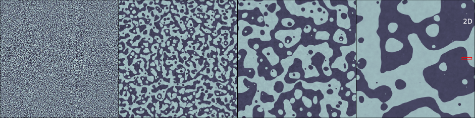
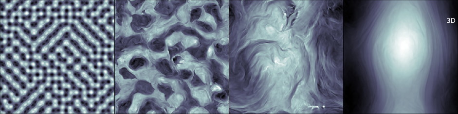
Figure 1.— Top: Two-dimensional turbulent relaxation in force-free electrodynamics at logarithmically spaced times ($t=0.08,0.32,1.28,5.12$). The initial condition is the $\alpha_{0}=256$ ABC field with $B_{1}=1,B_{2}=1,B_{3}=0$ and grid resolution $3072^{2}$. Shown is the out-of-plane magnetic field component scaled linearly between the initial minimum and maximum values. The small red rectangle overlying the right-most panel is the region shown amplified in Figure 4. The end-state is not a linear force-free equilibrium. Bottom: Three-dimensional turbulent relaxation under the same conditions except that $\alpha_{0}=16$, the grid resolution is $512^{3}$, and the times $t=0.625,1.0,3.0,16.0$ are chosen to elucidate the sequence of decay epochs. The color mapping accomodates the instantaneous data range, as it decreases appreciably throughout the decay. The end-state is a linear force-free equilibrium with $\alpha=1$.

Since the Lorentz force density vanishes in FFE, no $\mathbf{E}\cdot\mathbf{J}$ work is done on the charge carriers and the system is formally energy conserving. Nevertheless, time-dependent solutions may develop regions in which the condition $E<B$ is violated, i.e. no frame exists in which the electric field vanishes. This indicates a breakdown of the ideal force-free assumption, and the Ohm’s law given by Equation 3 must be modified. Although non-ideal force-free Ohm’s laws have been proposed in the literature (Gruzinov, 2007; Li et al., 2012), it is still commonplace to evolve the ideal system until such a breakdown occurs, and when it does to simply reduce the magnitude of $\mathbf{E}$ to prevent $E>B$. The physical motivation for this prescription, which we use here, is that energy is being radiated away when charges are accelerated to short out the electric field and restore $E<B$. The numerical evolution scheme is described in more detail in Section 3.1, and in Appendix A we confirm that it yields numerical convergence of the energy dissipation rate.

2.2. Topology

Force-free electrodynamics shares the same magnetic topological invariants as Newtonian and relativistic MHD, the lowest order of which is the total magnetic helicity given by Equation 1. Its invariance can be seen as stemming from the conservation of magnetic flux through a closed field loop, which is why it is commonly referred to as characterizing the interlocking of the magnetic field. Although the helicity density $\mathbf{A}\cdot\mathbf{B}$ depends on the choice of gauge, its integral $H_{\mathcal{V}}$ over any volume $\mathcal{V}$ bounded by magnetic surfaces is well-defined, and also invariant under ideal evolutions, such as Faraday’s law, when $\mathbf{E}\cdot\mathbf{B}=0$ (e.g. Brandenburg & Subramanian, 2005),

$$\partial_{t}H_{\mathcal{V}}=-2\int_{\mathcal{V}}\mathbf{E}\cdot\mathbf{B}d^{3}x.$$ (5)

Equation 5 implies that $H_{\mathcal{V}}$ can still be conserved approximately in the presence of non-ideal processes, as long as the volume in which they occur is small.

In principle, a domain that admits a partitioning by magnetic surfaces has an independently conserved helicity associated with each smaller volume. But in practice, three dimensional field geometries are too complex for such a partitioning to be possible. This is what led Taylor to conclude that relaxation is only constrained by a single topological invariant — the total helicity. The story is different in two dimensions since the magnetic surfaces are far simpler; their cross-sections are nested closed curves in the $x-y$ plane, and the helicity enclosed by each functions as an independently conserved quantity for as long as that surface retains its identity. But non-ideal effects, however small, permit the surfaces to merge with one another, erasing their identities and shuffling up their conserved helicities. Nevertheless, in two dimensions we can still construct a robust topological invariant that is far stricter than the total helicity.

We recall that in the presence of $z$-translational symmetry, the in-plane magnetic field is tangent to the isocontours of the magnetic flux function $A_{z}$. So each sub-volume $\mathcal{V}_{i}(\psi)$ in which $A_{z}>\psi$ is associated with a conserved helicity $\mathcal{H}_{i}(\psi)=\int_{\mathcal{V}_{i}(\psi)}\mathbf{A}\cdot\mathbf{B}d^{3}x$. To whatever extent the helicities of such volumes remain additive with respect to reconnections between their bounding surfaces, the sum $\mathcal{H}(\psi)=\sum_{i}\mathcal{H}_{i}(\psi)$ must be a robust topological invariant. This assumption is justified by Equation 5 when the non-ideal regions (where $\mathbf{E}\cdot\mathbf{B}\neq 0$) are small. Alternatively, consider the helicity (e.g. Berger & Field, 1984)

$$\mathcal{H}_{12}=2\Phi_{1}\Phi_{2}$$ (6)

of two flux tubes that are once-linked and independently non-helical. An example is a cylindrical structure whose external, toroidal flux $\Phi_{2}$ wraps an interior, poloidal flux $\Phi_{1}$. Two such structures that were joined to share an outer surface would then enclose a poloidal flux $2\Phi_{1}$, which is wrapped by the same toroidal flux $\Phi_{2}$. So, to whatever extent the “joining” is done without destroying magnetic flux, the resulting arrangement has a helicity $2\mathcal{H}_{12}$.

The presence of additional invariants $\mathcal{H}(\psi)$ is expected to place a more restrictive lower bound on the magnetic energy than would the total helicity $H$ alone. In particular, given that Taylor states of the same helicity but different wavelength will generally span a distinct range of $\psi$ values, there may be no way for one 2D linear equilibrium to evolve into another of a different wavelength while leaving $\mathcal{H}(\psi)$ unchanged. With this in mind, we anticipate that fully relaxed 2D states will have an energy that exceeds the Taylor minimum of $\alpha_{0}H/2$. We will describe the numerical determination of $\mathcal{H}(\psi)$ in Section 3.3, and in Section 4.3 we confirm that it is conserved by directly measuring it in our 2D simulations.

There is also the question of what should happen to configurations in which $H=0$ but $\mathcal{H}(\psi)\neq 0$, since such a configuration could not attain arbitrarily low energy while respecting each of the invariants $\mathcal{H}(\psi)$. Although behavior like this may be entirely possible, the particular initial conditions used in this study (described in Section 3.2 and summarized in Table 1) generally have values of $|\mathcal{H}(\psi)|$ that are much smaller than $2U_{B}/\alpha_{1}$, so we have not been able to observe it yet. Indeed, we will see in Section 4.2 that our 2D states with zero net helicity still decay toward very small energy.

3. Methods

We simulate magnetically dominated, relativistic turbulence on a periodic domain of length $L=2\pi$ in either two or three dimensions, using solutions of the ideal force-free electrodynamics equations, given by Equation 3 and Equation 4.

3.1. Numerical scheme

We evolve the FFE system using a fourth-order finite difference scheme. We use standard fourth-order difference operators to evaluate all the field gradients, and standard fourth-order Runge-Kutta time-stepping to advance the solution in time.

The FFE system requires three vector constraints to be maintained: no monopoles $\nabla\cdot\mathbf{B}=0$, perfect conductivity $\mathbf{E}\cdot\mathbf{B}=0$, and the existence of a frame in which $\mathbf{E}$ vanishes $E<B$. The first two constraints are formally preserved by FFE, but can be violated numerically at the level of truncation error. Our scheme maintains the solenoidal constraint using the hyperbolic divergence cleaning scheme proposed by Dedner et al. (2002), and later used in FFE simulations (e.g. Palenzuela et al., 2010). This amounts to supplementing Faraday’s law with a magnetic monopole current $\mathbf{J}_{B}=-\nabla\Psi$, where the scalar field $\Psi$ evolves according to the damped wave equation $\partial_{t}\Psi=-\nabla\cdot\mathbf{B}-\tau^{-1}\Psi$ with $\tau$ being a non-physical time scale for quenching the magnetic monopole. $\mathbf{E}\cdot\mathbf{B}=0$ is maintained exactly by disregarding the part of the truncation error that would give rise to a component of $\mathbf{E}$ in the direction of $\mathbf{B}$. Numerical noise introduced by finite difference operations can lead to unphysical growth of modes whose wavelengths are comparable to the numerical grid spacing. Our scheme suppresses these unphysical modes using Kreiss-Oliger dissipation, a form of low-pass filtering. Each of the procedures just mentioned supplements the FFE equations with terms at or below the level of the truncation error, so they do not modify the formal convergence order of our numerical scheme.

This numerical scheme was used in East et al. (2015), and convergence results, as well as comparisons to relativistic MHD simulations and analytical methods can be found in that reference. It has been implemented as part of the Mara (Zrake & MacFadyen, 2011) suite of relativistic turbulence codes, which has many run-time post-processing capabilities that allow us to perform spectral and statistical analysis of the solution at a high cadence while minimizing strain on the host architecture’s filesystem.

3.2. Initial conditions

We start our simulations with a monochromatic magnetic field, where all the power is at a single wavenumber magnitude $\alpha_{0}$, and with a vanishing electric field. The general expression for our initial conditions is

$$\mathbf{B}(\mathbf{x}) = \sum_{|\mathbf{k}|=\alpha_{0}}(\alpha_{0}\mathbf{\Psi}_{\mathbf{k}}+\epsilon i\mathbf{k}\times\mathbf{\Psi}_{\mathbf{k}})e^{i\mathbf{k}\cdot\mathbf{x}}$$ (7)

$$\mathbf{k}\cdot\hat{\mathbf{\Psi}}_{\mathbf{k}} = 0$$

$$\hat{\mathbf{\Psi}}_{\mathbf{k}} = \hat{\mathbf{\Psi}}_{-\mathbf{k}}^{*}$$

where the parameter $\epsilon$ is chosen to be either one or zero, corresponding to helical or non-helical configurations, respectively. Helical initial configurations where $\alpha_{0}>1$ are unstable equilibria (see Section 4.1), whereas the non-helical configurations are out of equilibrium. Some of our initial conditions are randomized, having $\mathbf{\Psi}_{\mathbf{k}}=\hat{\mathbf{e}}_{\mathbf{k}}e^{i\phi_{\mathbf{k}}}$ where $\hat{\mathbf{e}}_{\mathbf{k}}$ is a random unit vector in the plane orthogonal to $\mathbf{k}$ and $\phi_{\mathbf{k}}$ is a random phase. We also make use of a special case of Equation 7 known as the “ABC” solution (Arnold, 1965; Dombre et al., 1986). In general this is given by

$$\mathbf{B}^{\rm{ABC}}(\mathbf{x})=\begin{pmatrix}B_{3}\cos\alpha_{0}z-B_{2}\sin\alpha_{0}y\\ B_{1}\cos\alpha_{0}x-B_{3}\sin\alpha_{0}z\\ B_{2}\cos\alpha_{0}y-B_{1}\sin\alpha_{0}x\\ \end{pmatrix},$$ (8)

which is highly ordered and fully helical, meaning that $\mathbf{B}=\alpha_{0}\mathbf{A}$ (in the Coulomb gauge). In this study we will make frequent use of the case with $B_{1}=B_{2}=1$ and $B_{3}=0$, which we refer to as the 2D ABC configuration.

Our results are based on simulations having a range of initial frequencies $\alpha_{0}$ and numerical resolutions — which we will refer to by the number of grid points in each linear dimension $N$. In general, the quality of our results improves when we are able to simulate larger values of $\alpha_{0}$ with more separation between the initial length scale and the domain length scale. However, features (of size $\alpha_{0}^{-1}$) in our initial condition need to be resolved by a certain number of grid points in order to obtain robust solutions. In Appendix A we show that 32 cells per $\alpha_{0}^{-1}$ are sufficient to keep the error in the global helicity conservation smaller than 1%. In 2D we will present simulations with $\alpha_{0}$ as large as 256, with resolutions up to $16384^{2}$. In 3D, we will present simulations with $\alpha_{0}$ as large as 48 and resolution $1024^{3}$.

3.3. Diagnostics

We define the power spectral density of the electric, magnetic, and helicity fields, respectively, as

$$P_{E}(k_{i}) = \frac{1}{\Delta k_{i}}\sum_{k_{i}<|\mathbf{q}|<k_{i}+\Delta k_{i}}\mathbf{E}_{\mathbf{q}}\cdot\mathbf{E}^{*}_{\mathbf{q}}/2,$$ (9)

$$P_{B}(k_{i}) = \frac{1}{\Delta k_{i}}\sum_{k_{i}<|\mathbf{q}|<k_{i}+\Delta k_{i}}\mathbf{B}_{\mathbf{q}}\cdot\mathbf{B}^{*}_{\mathbf{q}}/2,$$

$$P_{H}(k_{i}) = \frac{1}{\Delta k_{i}}\sum_{k_{i}<|\mathbf{q}|<k_{i}+\Delta k_{i}}\mathbf{A}_{\mathbf{q}}\cdot\mathbf{B}^{*}_{\mathbf{q}}$$

where $\mathbf{E}_{\mathbf{q}}$, $\mathbf{B}_{\mathbf{q}}$, and $\mathbf{A}_{\mathbf{q}}$ are, respectively, the electric field, magnetic field, and vector potential Fourier harmonics of wavenumber $\mathbf{q}$. We normalize the Fourier harmonics so that the volume integrated electric and magnetic field energies $U_{E}$ and $U_{B}$, and the magnetic helicity $H$ are given by

$$U_{E}=\sum_{i}P_{E}(k_{i})\Delta k_{i},$$

$$U_{B}=\sum_{i}P_{B}(k_{i})\Delta k_{i},$$

$$H=\sum_{i}P_{H}(k_{i})\Delta k_{i}.$$

We also define the characteristic frequency of each field $k_{E}$, $k_{B}$, and $k_{H}$ as

$$k_{X}=\frac{\sum_{i}{P_{X}(k_{i})k_{i}\Delta k_{i}}}{\sum_{i}{P_{X}(k_{i})}\Delta k_{i}}$$ (10)

where $X$ is one of $E$, $B$, or $H$. The most probable wavenumber, where $P_{X}(k)$ is maximal, is denoted by $\tilde{k}_{X}$.

In two dimensions, we track the “helicity mass” function discussed in Section 2.2,

$$\mathcal{H}(\psi)=\int\Theta(A_{z}(\mathbf{x})-\psi)\mathbf{A}\cdot\mathbf{B}d^{3}x,$$ (11)

where $\Theta$ is the Heavyside step function. In practice, this diagnostic is more easily computed as the “helicity density” function $d\mathcal{H}/d\psi$, which we calculate by binning the lattice points according to their value of $A_{z}$, and assigning the weight $\mathbf{A}\cdot\mathbf{B}$. We also create the volume distribution $d\mathcal{V}/d\psi$ by binning points according to $A_{z}$ with uniform weights, and the helicity distribution over volume $d\mathcal{H}/d\mathcal{V}=\frac{d\mathcal{H}}{d\psi}/\frac{d\mathcal{V}}{d\psi}$.

4. Results

Figure 1 shows the evolution of both two and three dimensional freely decaying force-free magnetic turbulence. Both of these calculations are initiated in the 2D ABC state, but the one on top takes place on a two-dimensional domain where translational symmetry is assumed in the $z$ direction, and the bottom one was given a low-level white-noise perturbation to break the $z$-symmetry. The left-most image shows the solution shortly after saturation of the linear instability that was recently observed in East et al. (2015), an overview of which is provided in Section 4.1. The difference between the two runs is visually evident. While the three-dimensional solution becomes increasingly smooth at late times, the two-dimensional one maintains a network of abrupt field reversals. These structures are force-free rotational current layers, and are examined in depth in Section 4.4. As we will see in Section 4.2, the total magnetic energy dissipated is dramatically greater in the three-dimensional case than in the two-dimensional case. Both runs show evidence of the inverse cascade; large-scale coherency of the magnetic field must result from dynamical transfer of some magnetic energy toward longer wavelengths since the initial spectrum is monochromatic around $k=\alpha_{0}$. The inverse cascade will be examined in detail in Section 4.6.

4.1. Linear instability of the excited Taylor states

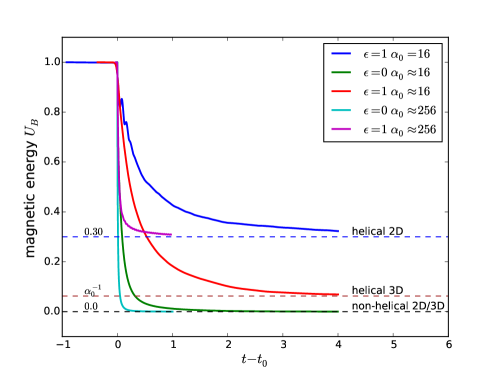
Figure 2.— Total magnetic energy $U_{B}$ as a function of time (since the onset of nonlinear evolution $t_{0}$). The energy of the terminal state takes on one of three values. In the case of two-dimensional helical evolution, the end-state contains coherent structures and retains $30\%$ of its initial energy, whereas for three-dimensional evolution the end-state is a longest wavelength Taylor state whose energy is reduced by a factor of $\alpha_{0}$ from its initial energy. When the decay is non-helical magnetic energy decays perpetually toward zero. The randomized initial condition $\alpha_{0}\approx 16$ corresponds to $\alpha_{0}^{2}=257$ and $\alpha_{0}\approx 256$ corresponds to $\alpha_{0}^{2}=65641$.

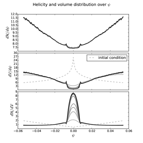
Figure 3.— Top — The helicity distribution $d\mathcal{H}/d\psi$ versus the level surface value $\psi$ of the magnetic potential function, shown at 16 evenly spaced times up to $t=16$ in a 2D ABC run with $\alpha_{0}=32$ and resolution $4096^{2}$. As anticipated in Section 2.2, $d\mathcal{H}/d\psi$ is essentially constant in time. Middle — The volume distribution $d\mathcal{V}/d\psi$, indicating the volume between level surfaces at a given $\psi$. The separatrix surfaces $\psi=0$ initially occupy the greatest volume, become the current layers, and end up with the smallest share of the volume. Bottom — The helicity per volume $d\mathcal{H}/d\mathcal{V}$. Lighter, wider curves indicate earlier time whereas darker, thinner curves indicate later times. The distributions are each normalized to unity.

Our helical initial conditions are linear force-free equilibria. Clearly they are stable when $\alpha_{0}=1$ since such states are global energy minima for a given magnetic helicity. The question of the ideal stability of the periodic shorter wavelength ($\alpha_{0}>1$) Taylor states has a conflicted history (e.g. Moffatt, 1986; Galloway & Frisch, 1987; Er-Riani et al., 2014), which has recently been resolved in East et al. (2015). In that study, numerical simulations of both FFE and relativistic MHD revealed that $\alpha_{0}>1$ Taylor states are linearly unstable to ideal perturbations. The instability is marked by exponential growth of the electric field on roughly the Alfvén wave crossing time of the initial structure size $\alpha_{0}^{-1}$, and saturates when the medium attains the Alfvén speed, which for the magnetically dominated case is $c$, implying the existence of regions where $E\approx B$. This instability affects generic states, and the only counter-examples that were found were one-dimensional ABC states (e.g. $B_{1}=1,B_{2}=0,B_{3}=0$) that are stable for all values of $\alpha_{0}$. Such states are pure plane waves having circular polarization, and are force-free by virtue of having uniform magnetic pressure. All of our helical initial conditions are short wavelength and either two or three dimensional, and turbulent relaxation begins after the saturation of the ideal instability.

4.2. Energy of fully relaxed configurations

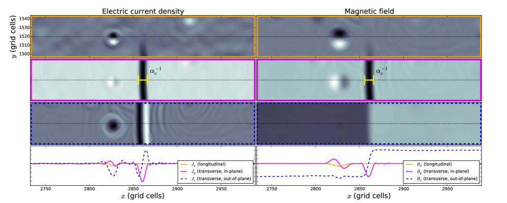
Figure 4.— Amplification of the small red rectangle overlying the rightmost panel of Figure 1, showing relief plots of the $x$, $y$, and $z$ components of the magnetic field (on the top three panels). The bottom panel shows one-dimensional profiles, taken along the horizontal centerline (dashed magenta).

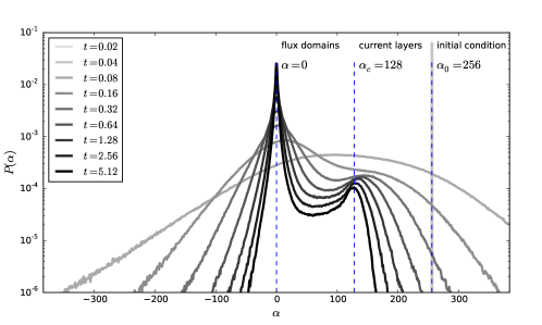
Figure 5.— Probability density function $P(\alpha)$ at logarithmically spaced times. The right-most vertical dashed line is the frequency $\alpha_{0}=256$ of the initial field configuration. The local maximum at $\alpha\approx 128$ is the frequency $\alpha_{c}$ of the current sheets (which is resolution dependent), and the maximum at $\alpha=0$ corresponds to zero-current characterizing the flux domain interiors.

Here we discuss the magnetic energy associated with the end-state magnetic configurations. Since the Taylor states have $\mathbf{B}=\alpha_{0}\mathbf{A}$, their energy is given simply by $\alpha_{0}H/2$. In other words, their energy is $\alpha_{0}$ times larger than the theoretical lower limit imposed by assuming the state reaches $\alpha=1$ at constant $H$. Whether or not dynamical relaxation processes settle with the field in this global energy minimum remains an open question, but here we provide some evidence to support the following conjecture: “force-free magnetic relaxation starting from periodic Taylor states ends in the lowest energy configuration allowed by helicity conservation if and only if the domain is three-dimensional.”

We have carried out a suite of calculations belonging to one of four categories, being either two or three dimensional, and either helical or non-helical. Those that are non-helical are, by construction, out of equilibrium at $t=0$ and could decay until they reach zero energy since helicity conservation does not place any lower bound on their magnetic energy. The helical ones are initially at an unstable equilibrium, enter a period of turbulent relaxation, and settle in a force-free equilibrium of lower energy. We considered initial conditions that are both of the randomized type given by Equation 7 and the ABC type given by Equation 8.

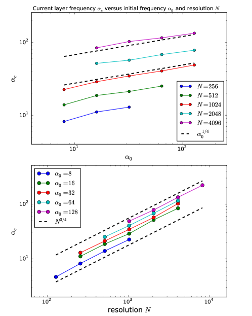
Figure 6.— Depenency of the current layer frequency $\alpha_{c}$ on the frequency $\alpha_{0}$ of the initial field configuration (top) and the grid resolution $N$ (bottom). $\alpha_{c}$ is defined to be the second local maximum (other than $\alpha=0$) in the probability density function $P(\alpha)$, where $\alpha=\mathbf{B}\cdot\nabla\times\mathbf{B}/B^{2}$.

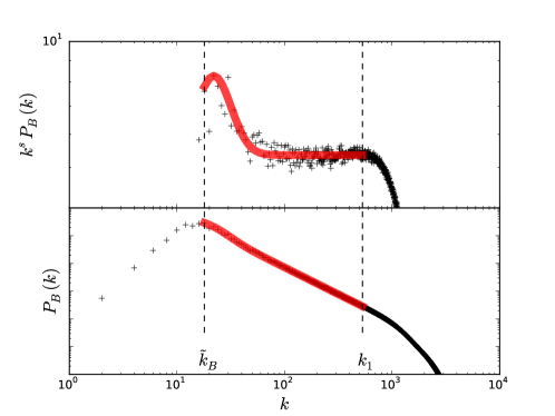
Figure 7.— Example best-fit (shown in red) to magnetic power spectrum data ($+$’s) for a two-dimensional helical model with $\alpha_{0}=256$ and resolution $16384^{2}$. $P_{B}(k)$ is shown compensated by the best-fit spectral index $s=1.94$ (top) and uncompensated (bottom). Vertical dashed lines indicate the window used for the fit, between the peak magnetic frequency $\tilde{k}_{B}$ and the spectral cutoff frequency $k_{1}$.

Our results are summarized in Figure 2, which shows the time series $U_{B}$ for each of six different runs. As expected, the non-helical configurations decay toward zero energy in both two and three dimensional settings. In three dimensions, the helical configurations all terminate in the lowest energy state allowed by helicity conservation . Both a randomized setup with $\alpha_{0}^{2}=257$ and the 2D ABC setup with $\alpha_{0}^{2}=256$ showed the same general behavior. The latter setup was intentionally chosen to be identical with the two-dimensional setup apart from the inclusion of a low-level (one part in $10^{8}$) white-noise perturbation introduced to break the $z$-translational symmetry.

Both of the helical two-dimensional runs terminate their relaxation with an energy that is decreased to only $30\%$ of its initial value. For example, a randomized 2D initial condition with $\alpha_{0}\approx 256$ settles in a state that has roughly 77 times more magnetic energy than the Taylor minimum energy state. This is not unique, as actually all of our helical 2D runs where $\alpha_{0}\gg 1$ (including $\alpha_{0}=16$) settle in a state whose energy is decreased to roughly $30\%$. In Appendix A we show that, for the 2D ABC $\alpha_{0}=256$ setup, the final energy is numerically converging to a value very near $30\%$. This means that the terminal states in two dimensions are not linear equilibria. In other words, they do approximately solve the force-free condition Equation 2, but the value of $\alpha$ may vary from one field line to another.

4.3. Helicity distribution

The fact that the 2D configurations do not relax into linear equilibria stems from invariance of the helicity distribution $\mathcal{H}(\psi)$ which we introduced in Section 2.2. Figure 3 confirms that it does indeed remain constant over time to a very good approximation, even while the volume distribution over the magnetic potential $d\mathcal{V}/d\psi$ changes significantly. The feature evident in the bottom panel of Figure 3, where in the relaxed state most of the volume is occupied by the extreme values of the magnetic potential, can be connected to the formation of current layers which we discuss in the next section.

As an illustration that invariance of the helicity distribution might prevent 2D relaxation from attaining longer wavelength linear equilibria, consider that the magnetic potential function $A_{z}$ of any 2D linear equilibrium satisfies

$$A_{z}=\left(\frac{H}{2\alpha_{0}L^{3}}\right)^{1/2}\frac{B_{z}}{\bar{B}_{z}}$$

where $\bar{B}_{z}$ is the root mean square value of $B_{z}$ and $H$ is the total helicity. $\mathcal{H}(\psi)$ can be characterized by its domain, namely the global maximum of $|A_{z}|$ which we denote by $\psi_{\rm{max}}$. For two different linear equilibria with frequencies $\alpha_{0}$ and $\alpha_{0}^{\prime}$ to have the same helicity distribution, it would be necessary for them to at least share the same values of $H$ and $\psi_{\rm{max}}$, requiring that

$$\left(\frac{\alpha_{0}}{\alpha_{0}^{\prime}}\right)^{1/2}=\frac{B_{z,\rm{max}}/\bar{B}_{z}}{B^{\prime}_{z,\rm{max}}/\bar{B}^{\prime}_{z}}.$$ (12)

where $B_{z,\rm{max}}$ is the global maximum of $|B_{z}|$. Note that in general, $\bar{B}_{z}\leq B_{z,\rm{max}}$. For the particular case of the 2D ABC state $B_{1}=B_{2}=1$, Equation 12 leads to the requirement that $\alpha_{0}^{\prime}\geq\alpha_{0}/2$, and therefore its relaxation into a linear state with twice smaller energy is impossible. In other words, there is no way for the 2D ABC state represented in Figure 3, whose $\alpha_{0}=32$, to evolve into another linear equilibrium whose frequency is smaller than $16$, while preserving $\mathcal{H}(\psi)$. We suspect this argument could be generalized further, but for now we leave it as a conjecture that the wavelength of a linear 2D equilibrium may be uniquely specified by its helicity distribution — which if true would render it impossible for one linear 2D equilibrium to relax into another of lower energy.

4.4. The current layers

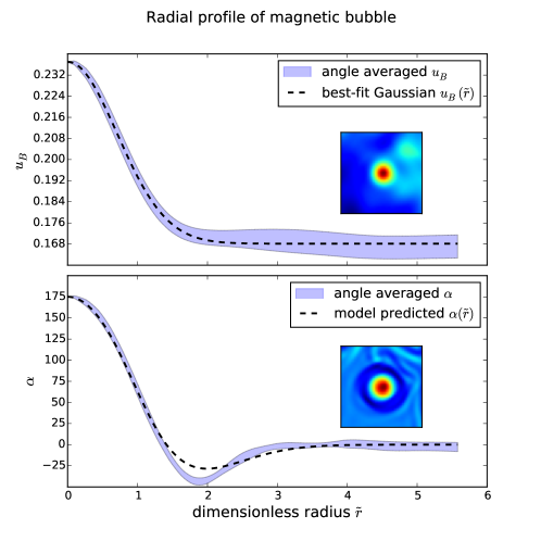
Figure 8.— Top — The magnetic pressure profile of a magnetic bubble in the dimensionless cylindrical radius $\tilde{r}=\alpha_{b}r$. The blue shaded region indicates the azimuthal standard deviation at each radius from the center, and the dashed line shows the best-fit model parameters for the Gaussian mangetic pressure enhancement given by Equation 15. Bottom — The azimuthally averaged value of $\alpha$ along with its predicted value (dashed line) given by Equation 16. The top and bottom insets show two-dimensional relief plots of $u_{B}$ and $\alpha$, respectively.

During the turbulent relaxation of helical two-dimensional configurations, the solution consists of oppositely signed flux domains separated from one another by a network of rotational force-free current layers. The flux domains (black and white regions of Figure 1) have nearly uniform $B_{z}$ and are thus relatively current-free. Across the current layers, the magnetic field direction rotates through approximately $180^{\circ}$, while its magnitude (and thus magnetic pressure) remains fixed. One such current layer is shown in Figure 4, where a one-dimensional profile has been taken along the $x$-axis, passing through the layer where it is aligned with the $y$-axis.

It is evident that the current layers have a characteristic frequency, which we denote by $\alpha_{c}$ and determine empirically as follows. Since the solution is near a force-free equilibrium, the current is $\mathbf{J}\approx\alpha\mathbf{B}$ for some spatially dependent frequency

$$\alpha=\mathbf{B}\cdot\nabla\times\mathbf{B}/B^{2}.$$

We anticipate that the probability density function $P(\alpha)$ will have two local maxima — one at $\alpha=0$ corresponding to the potential flux domain interiors and the other at the frequency $\alpha_{c}$, marking the frequency of the current layers. Figure 5 confirms this to be the case. It shows $P(\alpha)$ at logarithmically spaced times throughout the relaxation, and reveals the location of the second peak once the solution is sufficiently close to a force-free equilibrium. For this particular run, with $\alpha_{0}=256$ and $N=3072$, the value of $\alpha_{c}\approx 128$.

It turns out to be a coincidence that in this case $\alpha_{c}\approx\alpha_{0}/2$. We have performed a family of calculations, varying $\alpha_{0}$ between 8 and 128, and varying $N$ between 128 and 8192. For each run, we recorded the value of $\alpha_{c}$, time-averaged over roughly 100 snapshots between time $t=10$ and $t=16$, which was late enough that the second peak in $P(\alpha)$ had emerged in each run. There was no secular evolution of $\alpha_{c}$. Figure 6 reveals that current layers become increasingly narrow with higher resolution, but also with increasing initial frequency $\alpha_{0}$. The scaling is consistent with the expression

$$\alpha_{c}=k_{1}^{3/4}\alpha_{0}^{1/4}$$ (13)

where $k_{1}=N/30$ is the turbulence cutoff frequency, which has been determined by modeling the magnetic energy spectrum, (see Figure 7) and is insensitive to initial conditions, depending only on the numerical scheme and grid resolution. We emphasize that Equation 13 is strictly empirical, in that it matches the data shown in Figure 6.

The scaling given by Equation 13 indicates that in the infinite resolution limit, the current layers will have zero characteristic length. We are not able to say whether the scaling could be associated with a physical property of 2D FFE at finite Reynolds number, or if it might depend on the details of the numerical scheme. This question could be resolved by imposing the turbulence cutoff frequency $k_{1}$ explicitly, and then varying the numerical resolution. In other words, solutions to a resistive FFE system at a given conductivity parameter will be necessary.

4.5. Solitary magnetic bubbles

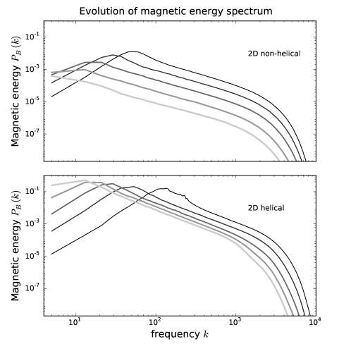
Figure 9.— Magnetic energy spectra $P_{B}(k)$ shown at logarithmically spaced times for a 2D simulation of freely decaying force-free turbulence. Randomized initial conditions with $\alpha_{0}\approx 256$ and $N=16384$, where $\epsilon=0$ (non-helical) on top and $\epsilon=1$ (helical) on bottom.

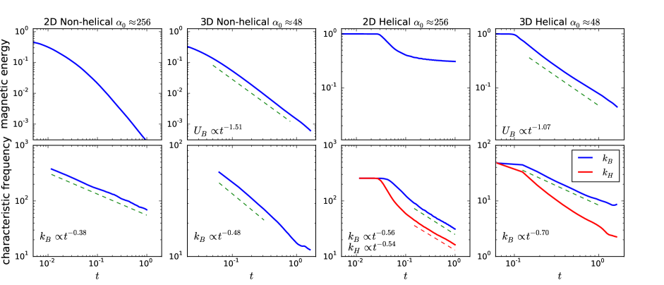
Figure 10.— Total magnetic energy $U_{B}$ as a function of time (top row) and evolution of the magnetic frequency $k_{B}$ and, for the helical runs, the helicity frequency $k_{H}$ (bottom row). One representative run is chosen from each of the four settings — 2D/3D non-helical, and 2D/3D helical.

The flux domain interiors contain another type of coherent structure. They are long-lived bubbles of toroidal magnetic field that are confined by ambient magnetic pressure. The circular object to the left of the current layer in Figure 4 is an example. They may be referred to as flux tubes or magnetic vortices, but we will refer to them as magnetic bubbles since we believe they are similar objects to those studied by Gruzinov (2010). The bubbles are helical, force-free magnetic field structures, having $\mathbf{J}$ very well aligned with $\mathbf{B}$. But they are not linear equilibria; the value of $\alpha$ varies with distance $r$ from the axis, and all the bubbles we examined had similar radial profiles $\alpha(r)$. The current flow is parallel to the background magnetic field near the core, but an equal and opposite return current flows through the sheath. So they could also be thought of as co-axial electric current channels oriented along the symmetry axis.

Force-free configurations with axial and $z$-symmetry satisfy the ordinary differential equations

$$B_{\phi}\alpha+B^{\prime}_{z}=0$$ (14)

$$B_{\phi}r^{-1}-B_{z}\alpha+B^{\prime}_{\phi}=0$$

where $\alpha(r)$ needs to be specified to make the solution unique, as well as the boundary conditions $B_{z}(r)\rightarrow B_{\infty}$ and $B_{\phi}(r)\rightarrow 0$ as $r\rightarrow\infty$. Requiring the total current $I=\int B_{\phi}rd\phi$ to be zero only forces $B_{\phi}(r)$ to decrease faster than $1/r$. Alternatively, the magnetic pressure $u_{B}(r)$ may be specified instead of $\alpha(r)$. One simple assumption, consistent with measurements of the bubbles, is that the magnetic pressure enhancement, relative to the ambient pressure $B^{2}_{\infty}/2$, is Gaussian. This gives a pressure profile

$$u_{B}(\tilde{r})=\frac{1}{2}B^{2}_{\infty}(1+fe^{-\tilde{r}^{2}})$$ (15)

in the dimensionless radius $\tilde{r}=\alpha_{b}r$ for a bubble of radius $\alpha_{b}^{-1}$, where $f$ is the magnetic pressure enhancement relative to background and could be any positive number. The corresponding solution of Equation 14 is

$$B_{\phi}(\tilde{r}) = B_{\infty}f^{1/2}\tilde{r}e^{-\tilde{r}^{2}/2}$$

$$B_{z}(\tilde{r}) = B_{\infty}\sqrt{1+fe^{-\tilde{r}^{2}}(1-\tilde{r}^{2})}$$

which has the profile

$$\alpha(\tilde{r})=\alpha_{b}\frac{(2-\tilde{r}^{2})e^{-\tilde{r}^{2}/2}}{\sqrt{(1-\tilde{r}^{2})e^{-\tilde{r}^{2}}+f^{-1}}}.$$ (16)

In Figure 8 we show the radial profile of magnetic pressure, azimuthally averaged around the bubble’s axis. This is the same object depicted to the left of the current layer in Figure 4. We also show the expression given in Equation 15 with its best-fit model parameters. For this particular object, the best-fit fractional magnetic energy enhancement was $f=0.41$ and the best-fit inverse radius was $\alpha_{b}=162$. The lower panel of Figure 8 shows the radial profile of $\alpha$, and also the model predicted value given by Equation 16 with the best-fit parameters.

So far we have not detected these structures in 3D simulations, but that does not mean they never happen. It is crucial to address whether they are even stable in three dimensions, and if they are, then under what conditions they may be attractors.

4.6. The inverse cascade

The inverse cascade can be characterized by the rate with which the magnetic coherence scale $k_{B}^{-1}$ (Equation 10) migrates toward longer wavelengths. We observe inverse cascading in force-free electrodynamics for every setting we have considered, whether the turbulence is 2D or 3D, helical or non-helical. Figure 9 shows evolution of the magnetic energy spectrum $P_{B}(k)$ over time, for representative helical and non-helical runs in 2D. We note how in both cases, the remaining magnetic energy resides at an increasing scale over time. We also note the spectral energy density at long wavelengths to be an increasing function of time, indicating that selective decay of the short wavelength modes alone cannot explain growth of the spatial coherency. This further generalizes observations made of non-helical 3D MHD turbulence, in both Newtonian (Brandenburg et al., 2015) and relativistic (Zrake, 2014) settings.

Figure 10 shows the evolution of the characteristic magnetic frequency $k_{B}$ for one model from each of the four categories. For the helical runs we also show the evolution of the helicity frequency $k_{H}$. Except for the general feature that over time, both $k_{B}$ and $k_{H}$ move to smaller frequency, there is no single decay law that characterizes all these settings. Some runs exhibit power-law time dependence of $U_{B}$, $k_{B}$, or $k_{H}$, but not all. Power-law dependence is considered evidence of self-similarity in the relaxation process, meaning the solution evolves only by rescaling itself in space and time (e.g. Landau & Lifshitz, 1987). Self-similar evolution may occur when the characteristic scales are all sufficiently smaller than the domain size, so that processes around the coherence scale are not yet contaminated by the requirement of periodicity at the domain scale. For this reason, large values of $\alpha_{0}$, and thus high domain resolution, may be required for self-similarity to emerge. For 3D, freely decaying non-helical relativistic MHD turbulence, Zrake (2014) found power-law dependence of $k_{B}\propto t^{-2/5}$ for $\alpha_{0}\approx 48$ initial conditions. For the same conditions in FFE, $k_{B}$ evolves with a power-law index of $-0.48$, as shown in the second column of Figure 10. However, the dependence of $k_{B}$ on time is not convincingly power-law, indicating that a scale separation of $\alpha_{0}\approx 48$ may not be sufficient to yield a decisive measurement of the decay index. In the future, we plan to follow-up on this with higher resolution simulations.

In freely decaying 2D non-helical force-free turbulence with very high resolution ($12288^{2}$) and $\alpha_{0}\approx 256$, clear power-law behavior of $k_{B}$ is observed, with an index of $-0.38$. The helical 2D case is different. As shown in Figure 10 (column 3), the energy drops to its terminal value of $\approx 0.3U_{B}(t=0)$ long before $k_{B}^{-1}$ approaches the domain scale. At times later than $t=0.15$, the merging of flux domains (evident in Figure 1) moves magnetic energy to progressively larger scales while suffering slower and slower dissipative losses. During this epoch, the both the helicity and magnetic frequencies decay with a power-law index of roughly $-0.55$.

In general, freely decaying magnetic turbulence must exhibit an inverse cascade when the magnetic helicity is near maximal ($H\approx U_{B}/k_{B}$), if $\partial_{t}H=0$ is to be satisfied (Frisch et al., 1975; Christensson et al., 2001; Cho, 2011). However, the same conclusion cannot be drawn from magnetic helicity conservation alone when $H\ll U_{B}/k_{B}$, as is the case for our non-helical runs. Observation of the non-helical inverse cascade was thus seen as a surprise (Zrake, 2014; Brandenburg et al., 2015). It was suggested in Zrake (2014) that the non-helical inverse cascade may reflect the tendency for aligned current structures to attract one another. Brandenburg et al. (2015) found that net transfer of energy from small to large scales was about twice larger in helical than non-helical freely decaying Newtonian MHD turbulence.

4.7. Power spectrum of electric and magnetic energy

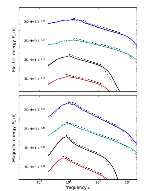
Figure 11.— Power spectra of the electric (top) and magnetic (bottom) energy densities as given by Equation 9 for one model from each of the catagories 2D/3D and helical/non-helical. The solid curves are measured from simulations of whose resolution is $16384^{2}$ in 2D and $1024^{3}$ in 3D, while the coinciding dash-dotted curves are measured from simulations whose resolution is slightly lower, $12288^{2}$ and $768^{3}$. Dashed lines indicate the best-fit parameters of Equation 17. An example fit is shown in more detail in Figure 7.

In all of our initial conditions the magnetic energy is concentrated around a single frequency, $P_{B}(k)\propto\delta(k-\alpha_{0})$. As turbulence develops, energy redistributes itself over all available scales, with the bulk of the energy around $k_{B}$ (which decreases over time as discussed in Section 4.6) and a power-law tail extending to the spectral cutoff frequency $k_{1}$ which lies consistently near $N/30$ when the grid resolution is $N$. We have determined the index $s$ of the power-law tail by fitting the logarithm of the spectral distributions $P_{E}(k)$ and $P_{B}(k)$ to the model function

$$f(x)=Ae^{-(x-x_{0})^{2}/2\sigma^{2}}+xs$$ (17)

where $x=\log k$, and $A$, $x_{0}$, $\sigma$, and $s$ are model parameters. We have found it expedient not to try and model the high-frequency cutoffs, we just use frequency bins between the peak frequency $\tilde{k}_{B}$ and the cutoff $k_{1}$ to obtain our fit. A representative spectral fit is shown in Figure 7.

Figure 11 shows $P_{E}(k)$ and $P_{B}(k)$ for one model from each of the categories 2D/3D and helical/non-helical along with the best-fit model given by Equation 17. We use randomized initial conditions for each model, and the resolution is $16384^{2}$ in 2D and $1024^{3}$ in 3D (coinciding dash-dotted curves are taken from simulations whose resolution is $12288^{2}$ and $768^{3}$ to indicate numerical consistency). The spectra represent the solution at an intermediate time, when $k_{B}\approx 8$, and we find the power-law indices to be quite stable during a window of time beginning on the snapshot chosen for each model. The power-law index of the electric field spectral energy distribution $P_{E}(k)$ is between 0.96 and 1.18 for the various models, with both of the helical models having an index of 1.18. The power-law index of the magnetic field spectral energy distribution $P_{B}(k)$ is different in two and three dimensions. In both helical and non-helical 3D settings, it is notably close to the Kolmogorov value of 5/3. Note that Zrake (2014) and Brandenburg et al. (2015) both measured an index near 2 for freely decaying non-helical MHD turbulence. The helical 2D model has an index of 1.93, and it is tempting to conclude that the true value is 2, but actually the best-fit parameter, for all resolutions up to $16384^{2}$ is significantly smaller than 2, always being between 1.92 and 1.96. The non-helical 2D model is found to have an index of 1.41.

5. Discussion and conclusions

Using high resolution simulations of the force-free electrodynamics equations, we have studied freely decaying, magnetically dominated relativistic turbulence for the first time. We focused on various differences between the magnetic relaxation process in settings where the domain is two and three dimensional, and where the magnetic field is helical and non-helical. We found that helical, two-dimensional relaxation terminates in a state whose energy is far above the theoretical minimum imposed by helicity conservation, and whose volume is predominantly current-free, but is punctuated by coherent structures — namely current layers and solitary magnetic bubbles. We tried to determine what sets the width of the current layers, and determined that it depends not only on the turbulence cutoff frequency (or grid resolution), but also on the frequency $\alpha_{0}$ of the initial condition. The solitary magnetic bubbles are axisymmetric, non-linear force-free equilibria, and are consistent with Gaussian magnetic pressure enhancement relative to the surrounding relatively current-free volume. The three-dimensional stability of these structures remains an open question.

The unusual behavior of 2D relaxations can be understood in terms of additional topological constraints that are imposed by the extra symmetry. We proposed that unlike generic 3D relaxation, whose topology is only constrained by the total helicity invariant $H$, 2D relaxations are subject to a whole spectrum of helicity invariants $\mathcal{H}(\psi)$, one associated with each value of the magnetic potential $\psi$. Although this invariance is only guaranteed when magnetic reconnections are restricted to regions of zero volume, our simulation data showed that $\mathcal{H}(\psi)$ remains unchanged throughout the evolution to a very good approximation.

All of the settings we considered exhibited inverse cascading, in which some magnetic energy is redistributed toward progressively longer wavelengths. The rate of inverse cascading was characterized by the time evolution of the magnetic frequency $k_{B}$, which was found to decrease faster when the field is helical than non-helical, and also faster in 3D than in 2D. The inverse cascade of 2D helical turbulence is nearly conservative; merging of magnetic flux domains moves energy to larger scales while suffering a diminishing rate of dissipative losses. The non-helical inverse cascade has $k_{B}\propto t^{-0.38}$ in 2D and $k_{B}\propto t^{-0.48}$ in 3D, in rough agreement with results of Zrake (2014) for 3D turbulent relaxation in relativistic MHD. Better scale separation (larger $\alpha_{0}$) and thus higher numerical resolution is needed to confirm the three dimensional scaling measurement.

5.1. Astrophysical gamma-ray sources and magnetoluminescence

We have examined turbulent relaxation in force-free electrodynamics with the motivation of elucidating the physical mechanism behind extremely fast time variability that is characteristic of astrophysical gamma-ray emitters, including the Crab Nebula, many blazars, and nearly all gamma-ray bursts. The extreme energetics and temporal intermittency of gamma radiation from these sources require a mechanism in which plasma promptly converts the majority of its magnetic energy into high energy particles and radiation. Furthermore, the emitting regions are thought to be strongly magnetized, and known to lie a great distance from the primary mover (pulsar, progenitor star, or black hole). These facts are highly suggestive that electromagnetic outflows may contain persistent magnetic structures with copious free energy supplies, whose spontaneous disruption could be linked to the observed flaring events. A scenario like this was referred to in Blandford et al. (2014) as magnetoluminescence. For it to be plausible, it is necessary that (1) meta-stable, force-free (or hydromagnetic) equilibria can exist far from any supporting boundaries, (2) that such objects can form under realistic astrophysical conditions, and (3) that upon their disruption, magnetic energy is promptly and completely dissipated.

In this paper, we have begun to address the points (1) and (3) and found results that are at least partially encouraging. All of our periodic 3D simulations exhibit prompt relaxation into the Taylor minimum energy state, supporting the idea that magnetic energy can be dissipated completely in a light-travel time. But the same result suggests that persistent, meta-stable structures are not a generic outcome of turbulence in force-free electrodynamics. This is not to say that such behavior is impossible, as we have only considered a small class of initial conditions. In fact, Smiet et al. (2015) very recently identified magnetic arrangements that on 3D periodic domains, in full MHD, relax to non-linear hydromagnetic equilibria. So (1) is possible, at least in the hydromagnetic case. The volatility of such objects, and the generality of conditions under which they may arise remain important questions for the future.

5.2. Comparison with other studies of magnetic relaxation

In this study we have begun to address the question of whether relativistic, force-free magnetic relaxation on periodic domains generically ends in a Taylor state, and found evidence to support the view that it does, provided the domain is three dimensional. But thus far we have only considered a restricted class of initial conditions — namely isotropic, monochromatic fields that are either linear force-free equilibria (helical) or completely non-helical.

Several studies in full MHD have now identified settings that relax to more general hydromagnetic equilibria for which $\mathbf{J}\times\mathbf{B}=\nabla p$, where the Lorentz force density balances the gradient of gas pressure $p$. Examples include stratified three-dimensional environments (Braithwaite, 2006, 2008) where the field is helical, and two-dimensional periodic settings where the field is incompressible and non-helical (Gruzinov, 2009). Amari & Luciani (2000) and Braithwaite (2015) have both provided examples of 3D hydromagnetic relaxation which first develop current layers, and then proceed to a smooth configuration via resistive processes. Both studies used boundary conditions where at least one of the directions was not periodic. Very recently, Smiet et al. (2015) has found instances of 3D hydromagnetic relaxation ending in smooth, non-linear equilibria with non-uniform pressure, even when the boundary is periodic or open. Such boundary conditions are highly relevant for the astrophysical processes mentioned in Section 5.1, and an important question is whether their results possess any force-free analogues. In particular, if stable and non-linear force-free equilibria do exist in 3D away from boundaries, then how likely are they to arise under realistic astrophysical conditions?

5.3. Effects of imposing extra symmetries in astrophysical simulations

Many studies of relativistic plasma and MHD processes are carried out assuming either translational or rotational symmetry, including simulations of force-free electrodynamics (McKinney, 2006b; Tchekhovskoy et al., 2008), relativistic MHD (Barkov & Komissarov, 2008; Komissarov et al., 2009; Komissarov & Barkov, 2009; Mizuno et al., 2011), and particle-in-cell (PIC) simulations (Spitkovsky, 2008; Keshet et al., 2009). As we have seen, 2D magnetic relaxations are far more topologically constrained, and persist in configurations of much higher energy than equivalent 3D relaxations. Furthermore, axisymmetric calculations are expected to exhibit similar artificialities to the slab-symmetric ones studied here, since they both share the same topological simplifications. In particular, the axisymmetric magnetic surfaces, now toroidal shells that are labeled by their value of the azimuthal vector potential component $A_{\phi}$, each enclose a conserved magnetic helicity.

Our results indicate that as a field’s complexity increases, so does the discrepancy between the energy of its most relaxed state in 2D and 3D. So, axisymmetry may be appropriate when the field is near a stable force-free equilibrium, when little or no energy resides in higher-order radial or angular modes. But when these modes are populated, the imposed symmetry could make them artificially persistent.

Numerical studies of pulsar magnetospheres and magnetar flares are quite challenging, and much of the progress in this field has been obtained by restricting to axisymmetry. Simulations using both FFE (Parfrey et al., 2012; Yu, 2012; Parfrey et al., 2013) and PIC (Cerutti et al., 2015) show the development of complex structure in the meridional plane. Similarly, short wavelength toroidal magnetic structure has been found in axisymmetric FFE simulations of black hole accretion. For example the results of Parfrey et al. (2014) suggest that even disordered (as opposed to large-scale) magnetic fields advected inward by an accretion disk could facilitate angular momentum extraction from a black hole. The differences in 2D versus 3D found here suggest that extending these studies to be fully three dimensional, as that becomes computationally feasible, will be an exciting frontier, and will likely reveal qualitatively new dynamics.

Another setting where 2D and 3D calculations are expected to differ is shock-generated turbulence, which may account for the relatively high magnetizations inferred from non-thermal emission spectra of astrophysical shock fronts — both in non-relativistic settings such as supernova remnants and relativistic settings such as gamma-ray burst afterglows. Amplification of the magnetic field by turbulence in and around the shock, and its subsequent decay in the post-shock flow has been studied extensively in both two (Mizuno et al., 2011) and three (Inoue et al., 2010) dimensions with relativistic MHD, and also in 2D and 3D PIC simulations (Sironi & Spitkovsky, 2009; Sironi et al., 2013). In this study we have observed power-law decay of the magnetic energy in all settings, but with a steeper index in 3D than in 2D. This should be kept in mind, as even minor differences in the decay law can have an impact on the efficiency of first order Fermi processes (Lemoine et al., 2006; Niemiec & Ostrowski, 2006; Niemiec et al., 2006; Pelletier et al., 2009) as well as interpretations of GRB afterglows (Gruzinov & Waxman, 1999; Rossi & Rees, 2003; Lemoine, 2014).

Appendix A Numerical convergence

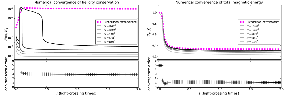
Figure 12.— Left - Error in the conservation of magnetic helicity $H$. The upper panel shows the fractional helicity change $\Delta h(t)=H(t)/H_{0}-1$ on symmetric logarithmic axes (to account for anomolous helicity change of either sign) for six different values of the mesh spacing $h$. The dashed magneta line shows the Richardson-extrapolated value of $\Delta h(t)$, which remains constant at roughly $10^{-3}$. The lower panel shows the convergence order of $\Delta h(t)$ at representative times. Right - Evolution of the total magnetic energy $U_{B}(t)$ for the same six values of the mesh spacing. The dashed magenta line on the upper panel shows the Richardson-extrapolated time series of $U_{B}(t)$, and the convergence order is shown on the lower panel.

Here we demonstrate some numerical convergence properties of our scheme. We have chosen the conservation of magnetic helicity $\Delta H(t)$ and the time series of magnetic energy $U_{B}(t)$ as diagnostics. Convergence properties are reported for the 2D helical runs with $\alpha_{0}=256$ and grid resolutions $4096^{2}$, $6144^{2}$, $8192^{2}$, $12288^{2}$ and $16384^{2}$. This configuration was found to be representative of convergence properties in other settings reported in this paper. All runs were evolved for at least two light-crossing times. In order to establish the numerical convergence order $n$, we model the error of the numerical solution $y_{h}$ with grid spacing $h$ as $y_{h}=y_{0}+Eh^{n}$ where $E$ is a constant and $y_{0}$ is the extrapolated solution. This is similar to a Richardson extrapolation, but instead of fitting for the coefficient $E_{n}$ for each integer power of $h$, we have fit for the single error coefficient $E$ and convergence order $n$.

The upper left panel of Figure 12 shows the fractional change in magnetic helicity $H(t)/H_{0}-1$ as a function of time for each resolution. For resolutions $>4096^{2}$, the helicity change is never worse than $\pm 10\%$. For $>8192^{2}$ it is never worse than $\pm 1\%$, and for $>12288^{2}$ it is never worse than $\pm 0.1\%$. The extrapolated value of the helicity change is consistently a gain of about $0.1\%$, and the convergence order (shown on the lower left panel of Figure 12) is between 2.8 and 2.9. The right panel shows the evolution of magnetic energy $U_{B}(t)$ at each resolution. Less dissipation occurs for each higher resolution, but the sequence converges consistently at first order. The extrapolated value of the magnetic energy at $t=2$ is 0.30, and it changes by less than $1\%$ between $t=1$ and $t=2$.

References

- Abdo et al. (2011) Abdo, A. A., Ackermann, M., Ajello, M., et al. 2011, Science (New York, N.Y.), 331, 739
- Aharonian et al. (2006) Aharonian, F., Akhperjanian, A. G., Bazer-Bachi, A. R., et al. 2006, Science (New York, N.Y.), 314, 1424
- Aharonian et al. (2007) —. 2007, The Astrophysical Journal, 664, L71
- Aleksić et al. (2014) Aleksić, J., Ansoldi, S., Antonelli, L. A., et al. 2014, Science (New York, N.Y.), 346, 1080
- Amari & Luciani (2000) Amari, T., & Luciani, J. F. 2000, Physical Review Letters, 84, 1196
- Arnold (1965) Arnold, V. 1965, Comptes rendus hebdomadaires des séances de l’Académie des sciences, 261, 17
- Banerjee & Jedamzik (2004) Banerjee, R., & Jedamzik, K. 2004, Physical Review D, 70, 123003
- Barkov & Komissarov (2008) Barkov, M. V., & Komissarov, S. S. 2008, Monthly Notices of the Royal Astronomical Society: Letters, 385, L28
- Bekenstein (1987) Bekenstein, J. D. 1987, The Astrophysical Journal, 319, 207
- Berger & Field (1984) Berger, M. A., & Field, G. B. 1984, Journal of Fluid Mechanics, 147, 133
- Blackman (2014) Blackman, E. G. 2014, Space Science Reviews, 188, 59
- Blackman & Field (2004) Blackman, E. G., & Field, G. B. 2004, Physics of Plasmas, 11, 3264
- Blandford et al. (2014) Blandford, R., Simeon, P., & Yuan, Y. 2014, Nuclear Physics B - Proceedings Supplements, 256-257, 9
- Blandford et al. (2015) Blandford, R., Yuan, Y., & Zrake, J. 2015, American Astronomical Society
- Blandford & Znajek (1977) Blandford, R. D., & Znajek, R. L. 1977, Monthly Notices of the Royal Astronomical Society, 179, 433
- Braithwaite (2006) Braithwaite, J. 2006, Astronomy and Astrophysics, 453, 687
- Braithwaite (2008) —. 2008, Monthly Notices of the Royal Astronomical Society, 386, 1947
- Braithwaite (2009) —. 2009, Monthly Notices of the Royal Astronomical Society, 397, 763
- Braithwaite (2015) —. 2015, Monthly Notices of the Royal Astronomical Society, 450, 3201
- Brandenburg et al. (2015) Brandenburg, A., Kahniashvili, T., & Tevzadze, A. G. 2015, Physical Review Letters, 114, 075001
- Brandenburg & Subramanian (2005) Brandenburg, A., & Subramanian, K. 2005, Physics Reports, 417, 1
- Cerutti et al. (2015) Cerutti, B., Philippov, A., Parfrey, K., & Spitkovsky, A. 2015, Monthly Notices of the Royal Astronomical Society, 448, 606
- Chandrasekhar & Fermi (1953) Chandrasekhar, S., & Fermi, E. 1953, The Astrophysical Journal, 118, 116
- Cho (2005) Cho, J. 2005, The Astrophysical Journal, 621, 324
- Cho (2011) —. 2011, Physical Review Letters, 106, 191104
- Cho & Lazarian (2014) Cho, J., & Lazarian, A. 2014, The Astrophysical Journal, 780, 30
- Christensson et al. (2001) Christensson, M., Hindmarsh, M., & Brandenburg, A. 2001, Physical Review E, 64, 056405
- Dedner et al. (2002) Dedner, A., Kemm, F., Kröner, D., et al. 2002, Journal of Computational Physics, 175, 645
- Dombre et al. (1986) Dombre, T., Frisch, U., Henon, M., Greene, J. M., & Soward, A. M. 1986, Journal of Fluid Mechanics, 167, 353
- Duez et al. (2010) Duez, V., Braithwaite, J., & Mathis, S. 2010, The Astrophysical Journal, 724, L34
- East et al. (2015) East, W. E., Zrake, J., Yuan, Y., & Blandford, R. D. 2015, Physical Review Letters, 115, 095002
- Er-Riani et al. (2014) Er-Riani, M., Naji, A., & El Jarroudi, M. 2014, International Journal of Non-Linear Mechanics, 67, 231
- Frisch et al. (1975) Frisch, U., Pouquet, A., Leorat, J., & Mazure, A. 1975, Journal of Fluid Mechanics, 68, 769
- Galloway & Frisch (1987) Galloway, D., & Frisch, U. 1987, Journal of Fluid Mechanics, 180, 557
- Goldreich & Julian (1969) Goldreich, P., & Julian, W. H. 1969, The Astrophysical Journal, 157, 869
- Goldreich & Sridhar (1995) Goldreich, P., & Sridhar, S. 1995, Astrophysical Journal, 438, 763
- Gralla et al. (2015) Gralla, S. E., Lupsasca, A., & Rodriguez, M. J. 2015, ArXiv e-prints, arXiv:1504.02113
- Gruzinov (2007) Gruzinov, A. 2007, arXiv, arXiv:0710.1875
- Gruzinov (2009) —. 2009, arXiv, arXiv:0909.1815
- Gruzinov (2010) —. 2010, arXiv, arXiv:1006.1368
- Gruzinov & Waxman (1999) Gruzinov, A., & Waxman, E. 1999, The Astrophysical Journal, 511, 852
- Hayashida et al. (2015) Hayashida, M., Nalewajko, K., Madejski, G. M., et al. 2015, The Astrophysical Journal, 807, 79
- Inoue et al. (2010) Inoue, T., Asano, K., & Ioka, K. 2010, arXiv, astro-ph.H
- Keshet et al. (2009) Keshet, U., Katz, B., Spitkovsky, A., & Waxman, E. 2009, The Astrophysical Journal Letters, 693, L127
- Komissarov & Barkov (2009) Komissarov, S. S., & Barkov, M. V. 2009, Monthly Notices of the Royal Astronomical Society, 397, 1153
- Komissarov et al. (2009) Komissarov, S. S., Vlahakis, N., Königl, A., & Barkov, M. V. 2009, Monthly Notices of the Royal Astronomical Society, 394, 1182
- Landau & Lifshitz (1987) Landau, L., & Lifshitz, E. 1987, Course of Theoretical Physics, 227
- Lazarian et al. (2003) Lazarian, A., Petrosian, V., Yan, H., & Cho, J. 2003, 18
- Lazarian & Vishniac (1999) Lazarian, A., & Vishniac, E. T. 1999, The Astrophysical Journal, 517, 700
- Lemoine (2014) Lemoine, M. 2014, arXiv:1410.0146
- Lemoine et al. (2006) Lemoine, M., Pelletier, G., & Revenu, B. 2006, The Astrophysical Journal, 645, L129
- Li et al. (2012) Li, J., Spitkovsky, A., & Tchekhovskoy, A. 2012, The Astrophysical Journal, 746, 60
- Lyutikov & Uzdensky (2003) Lyutikov, M., & Uzdensky, D. 2003, The Astrophysical Journal, 589, 893
- McKinney (2006a) McKinney, J. C. 2006a, Monthly Notices of the Royal Astronomical Society, 367, 1797
- McKinney (2006b) —. 2006b, Monthly Notices of the Royal Astronomical Society: Letters, 368, L30
- McKinney & Uzdensky (2012) McKinney, J. C., & Uzdensky, D. A. 2012, Monthly Notices of the Royal Astronomical Society, 419, 573
- Mizuno et al. (2011) Mizuno, Y., Pohl, M., Niemiec, J., et al. 2011, The Astrophysical Journal, 726, 62
- Moffatt (1986) Moffatt, H. K. 1986, Journal of Fluid Mechanics, 166, 359
- Niemiec & Ostrowski (2006) Niemiec, J., & Ostrowski, M. 2006, The Astrophysical Journal, 641, 984
- Niemiec et al. (2006) Niemiec, J., Ostrowski, M., & Pohl, M. 2006, The Astrophysical Journal, 650, 1020
- Olesen (1997) Olesen, P. 1997, Physics Letters B, 398, 321
- Palenzuela et al. (2010) Palenzuela, C., Garrett, T., Lehner, L., & Liebling, S. L. 2010, Physical Review D, 82, 044045
- Parfrey et al. (2012) Parfrey, K., Beloborodov, A. M., & Hui, L. 2012, The Astrophysical Journal, 754, L12
- Parfrey et al. (2013) —. 2013, The Astrophysical Journal, 774, 92
- Parfrey et al. (2014) Parfrey, K., Giannios, D., & Beloborodov, A. M. 2014, Monthly Notices of the Royal Astronomical Society: Letters, 446, L61
- Pelletier et al. (2009) Pelletier, G., Lemoine, M., & Marcowith, A. 2009, Monthly Notices of the Royal Astronomical Society, 393, 587
- Pfeiffer & MacFadyen (2013) Pfeiffer, H. P., & MacFadyen, A. I. 2013, 11
- Pontin et al. (2013) Pontin, D., Wilmot-Smith, A., & Hornig, G. 2013, Procedia IUTAM, 9, 110
- Rossi & Rees (2003) Rossi, E., & Rees, M. J. 2003, Monthly Notices of the Royal Astronomical Society, 339, 881
- Saito et al. (2013) Saito, S., Stawarz, ., Tanaka, Y. T., et al. 2013, The Astrophysical Journal, 766, L11
- Shats et al. (2005) Shats, M. G., Xia, H., & Punzmann, H. 2005, Physical Review E, 71, 046409
- Sironi & Spitkovsky (2009) Sironi, L., & Spitkovsky, A. 2009, The Astrophysical Journal, 698, 1523
- Sironi & Spitkovsky (2014) —. 2014, The Astrophysical Journal, 783, L21
- Sironi et al. (2013) Sironi, L., Spitkovsky, A., & Arons, J. 2013, The Astrophysical Journal, 771, 54
- Smiet et al. (2015) Smiet, C. B., Candelaresi, S., Thompson, A., et al. 2015, arXiv:1507.08780
- Son (1999) Son, D. 1999, Physical Review D, 59, 063008
- Spitkovsky (2006) Spitkovsky, A. 2006, The Astrophysical Journal, 648, L51
- Spitkovsky (2008) —. 2008, The Astrophysical Journal, 682, L5
- Tavani et al. (2011) Tavani, M., Bulgarelli, A., Vittorini, V., et al. 2011, Science (New York, N.Y.), 331, 736
- Taylor (1974) Taylor, J. B. 1974, Physical Review Letters, 33, 1139
- Tchekhovskoy et al. (2008) Tchekhovskoy, A., McKinney, J. C., & Narayan, R. 2008, Monthly Notices of the Royal Astronomical Society, 388, 551
- Thompson & Blaes (1998) Thompson, C., & Blaes, O. 1998, Physical Review D (Particles, 57, 3219
- Tobias et al. (2011) Tobias, S. M., Cattaneo, F., & Boldyrev, S. 2011, eprint arXiv, 1103, 3138
- Yang et al. (2015) Yang, H., Zhang, F., & Lehner, L. 2015, Phys. Rev. D, 91, 124055
- Yu (2012) Yu, C. 2012, The Astrophysical Journal, 757, 67
- Zhang & Yan (2011) Zhang, B., & Yan, H. 2011, The Astrophysical Journal, 726, 90
- Zhang et al. (2009) Zhang, W., MacFadyen, A., & Wang, P. 2009, The Astrophysical Journal, 692, L40
- Zrake (2014) Zrake, J. 2014, The Astrophysical Journal, 794, L26
- Zrake & MacFadyen (2011) Zrake, J., & MacFadyen, A. I. 2011, The Astrophysical Journal, 744, 32
- Zrake & MacFadyen (2013) —. 2013, The Astrophysical Journal, 769, L29