In-Network View Synthesis for Interactive Multiview Video Systems

Abstract

Interactive multiview video applications endow users with the freedom to navigate through neighboring viewpoints in a 3D scene. To enable such interactive navigation with a minimum view-switching delay, multiple camera views are sent to the users, which are used as reference images to synthesize additional virtual views via depth-image-based rendering. In practice, bandwidth constraints may however restrict the number of reference views sent to clients per time unit, which may in turn limit the quality of the synthesized viewpoints. We argue that the reference view selection should ideally be performed close to the users, and we study the problem of in-network reference view synthesis such that the navigation quality is maximized at the clients. We consider a distributed cloud network architecture where data stored in a main cloud is delivered to end users with the help of cloudlets, i.e., resource-rich proxies close to the users. In order to satisfy last-hop bandwidth constraints from the cloudlet to the users, a cloudlet re-samples viewpoints of the 3D scene into a discrete set of views (combination of received camera views and virtual views synthesized) to be used as reference for the synthesis of additional virtual views at the client. This in-network synthesis leads to better viewpoint sampling given a bandwidth constraint compared to simple selection of camera views, but it may however carry a distortion penalty in the cloudlet-synthesized reference views. We therefore cast a new reference view selection problem where the best subset of views is defined as the one minimizing the distortion over a view navigation window defined by the user under some transmission bandwidth constraints. We show that the view selection problem is NP-hard, and propose an effective polynomial time algorithm using dynamic programming to solve the optimization problem under general assumptions that cover most of the multiview scenarios in practice. Simulation results finally confirm the performance gain offered by virtual view synthesis in the network. It shows that cloud computing resources provide important benefits in resource greedy applications such as interactive multiview video.

I Introduction

Interactive free viewpoint video systems [1] endow users with the ability to choose and display any virtual view of a 3D scene, given original viewpoint images captured by multiple cameras. In particular, a virtual view image can be synthesized by the decoder via depth-image-based rendering (DIBR) [2] using texture and depth images of two neighboring views that act as reference viewpoints. One of the key challenges in interactive multiview video streaming (IMVS) [3] systems is to transmit an appropriate subset of reference views from a potentially large number of camera-captured views such that the client enjoys high quality and low delay view navigation even in resource-constrained environments [4, 5, 6].

In this paper, we propose a new paradigm to solve the reference view selection problem and capitalize on cloud computing resources to perform fine adaptation close to the clients. We consider a hierarchical cloud framework, where the selection of reference views is performed by a network of cloudlets, i.e., resource-rich proxies that can perform personalized processing at the edges of the core network [7, 8]. An adaptation at the cloudlets results in a smaller round-trip time (RTT), hence more reactivity than in more centralized architectures. Specifically, we consider the scenario depicted in Fig. 1, where a main cloud stores pre-encoded video from different cameras, which are then transmitted to the edge cloudlets that act as proxies for final delivery to users. We assume that there is sufficient network capacity between the main cloud and the edge cloudlets for the transmission of all camera views, but there exists however a bottleneck of limited capacity between a cloudlet and a nearby user. In this scenario, each cloudlet sends to a client the set of reference views that respect bandwidth capacities and enable synthesis of all viewpoints in the client’s navigation window. This window is defined as the range of viewpoints in which the user can navigate during the RTT and enables zero-delay view-switching at the client.

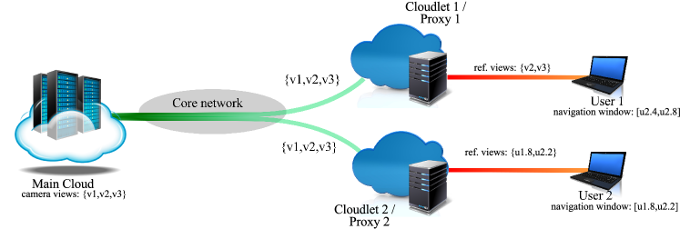
Figure 1: Considered scenario. Green lines represent no bandwidth constrained channels, red lines are bottleneck channels.

We argue that, in resource-constrained networks, re-sampling the viewpoints of the 3D scene in the network— i.e., synthesizing novel virtual views in the cloudlets that are transmitted as new references to the decoder—is beneficial compared to the mere subsampling of the original set of camera views. We illustrate this in Fig. 1, where the main cloud stores three coded camera views: $\{v_{1},v_{2},v_{3}\}$ while the bottleneck links between cloudlet-user pairs can support the transmission of only two views. If user 1 requests a navigation window $[u_{2.4},u_{2.8}]$, the cloudlet can simply forward the closest camera views $v_{2}$ and $v_{3}$. However, if user 2 requests the navigation window $[u_{1.8},u_{2.2}]$, transmitting camera views $v_{1}$ and $v_{3}$ results in large synthesized view distortions due to the large distance between reference and virtual views (called reference view distance in the sequel). Instead, the cloudlet can synthesize virtual views $u_{1.8}$ and $u_{2.2}$ using camera views $v_{1},v_{2},v_{3}$ and send these virtual views to the user 2 as new reference views for the navigation window $[u_{1.8},u_{2.2}]$. This strategy may result in smaller synthesized view distortion due to the smaller distance to the reference views. However, the in-network virtual view synthesis may also introduce distortion into the new reference views $u_{1.8}$ and $u_{2.2}$, which results in a tradeoff that should be carefully considered when choosing the views to be synthesized in the cloudlet.

Equipped with the above intuitions, we study the main tradeoff between reference distortion and bandwidth gain. Using a Gauss-Markov model, we first analyze the benefit of synthesizing new reference images in the network. We then formulate a new synthesized reference view selection optimization problem. It consists in selecting or constructing the optimal reference views that lead to the minimum distortion for all synthesized virtual views in the user’s navigation window subject to a bandwidth constraint between the cloudlet and the user. We show that this combinatorial problem can be solved optimally but that it is NP-hard. We then introduce a generic assumption on the view synthesis distortion which leads to a polynomial time solution with a dynamic programming (DP) algorithm. We then provide extensive simulation results for synthetic and natural sequences. They confirm the quality gain experienced by the IMVS clients when synthesis is allowed in the network, with respect to scenarios whose edge cloudlets can only transmit camera views. They also show that synthesis in the network allows to maintain good navigation quality when reducing the number of cameras as well as when cameras are not ideally positioned in the 3D scene. This is an important advantage in practical settings, which confirms that cloud processing resources can be judiciously used to improve the performance of applications that are a priori quite greedy in terms of network resources.

The remainder of this paper is organized as follows. Related works are described in Section II. In Section III, we provide a system overview and analyze the benefit of in-network view synthesis via a Gauss-Markov model to impart intuitions. The reference view selection optimization problem is then formulated in Section IV. We propose general assumptions on view synthesis distortion in Section V and derive an additional polynomial time view selection algorithm. In Section VI, we discuss the simulation results, and we conclude in Section VII.

II Related Work

Prior studies addressed the problem of providing interactivity in selecting views in IMVS, while saving on transmitted bandwidth and view-switching delay [9, 10, 11, 12, 13, 3, 14, 15]. These works are mainly focused on optimizing the frame coding structure to improve interactive media services. In the case of pre-stored camera views, however, rather than optimal frame coding structures, interactivity in network-constrained scenario can be addressed by studying optimal camera selection strategies, where a subset of selected camera views is actually transmitted to clients such that the navigation quality is maximized and resource constraints are satisfied [4, 16, 5, 17, 6, 18]. In [19], an optimal camera view selection algorithm in resource-constrained networks has been proposed based on the users’ navigation paths. In [20] a bit allocation algorithm over an optimal subset of camera views is proposed for optimizing the visual distortion of reconstructed views in interactive systems. Finally, in [21, 22] authors optimally organize camera views into layered subsets that are coded and delivered to clients in a prioritized fashion to accommodates for the network and clients heterogeneity and to effectively exploit the resources of the overlay network. While in these works the selection is limited to camera views, in our work we rather assume in-network processing able to synthesize virtual viewpoints in the cloud network.

In-network adaptation strategies allow to cope with network resource constraints and are mainly categorized in $i)$ packet-level processing and $ii)$ modification of the source information. In the first category, packet filtering, routing strategies [23, 24] or caching of media content information [25, 26] allow to save network resources while improving the quality experienced by clients. To better address media delivery services in highly heterogenous scenarios, network coding strategies for multimedia streaming have been also proposed [27, 28, 29]. In the second category — in-network processing at the source level — the main objective is usually to avoid transmitting large amounts of raw streams to the clients by processing the source data in the network to reduce both the communication volume and the processing required at the client side. Transcoding strategies might be collaboratively performed in peer-to-peer networks [30] or in the cloud [31]. Furthermore, source data can be compressed in the cloud [30, 32, 33] to efficiently address users’ requests. Rather than media processing in the main cloud, offloading resources to a cloudlet, i.e., a resource-rich machine in the proximity of the users, might reduce the transmission latency [7, 8]. This is beneficial for delay-sensitive / interactive applications [34, 35, 36]. Because of the proximity of cloudlets to users, cloudlet computing has been under intense investigation for cloud-gaming applications, as shown in [37] and references there in. The above works are mainly focused on multimedia processing, rather than on specific multiview scenarios. However, the use of cloudlets in delay sensitive applications motivates the idea of cloudlet-based view synthesis for IMVS.

Cloud processing for multiview system is considered in [38, 39, 40]. In [39] authors mainly address the cloud-based processing from a security perspective. In [40], view synthesis in the network has been introduced for cloud networks to offload clients’ terminals (in terms of complexity). The desired view is synthesized in the cloud and then sent directly to clients. However, only the view requested by the client is synthesized. This means that either the desired view is a priori known at the source or a switching delay is experienced by the clients. To the best of our knowledge, none of the work investigating cloud processing have considered the problem of multi-view interactive streaming under network resource constraints. In our work, we propose view synthesis in the network mainly to both overcome uncertainty of users’ requests in interactive systems and to cope with limited network resources.

III Background

III-A System Model

Let $\mathcal{V}=\{v_{1},\ldots,v_{N}\}$ be the set of the $N$ camera viewpoints captured by the multiview system. For all camera-captured views, compressed texture and depth maps are stored at the main cloud, with each texture/depth map pair encoded at the same rate using standard video coding tools like H.264[41] or HEVC[42]. The possible viewpoints offered to the users are denoted by $\mathcal{U}=\{u_{1},u_{1+\delta},\ldots,u_{N}\}$. The set $\mathcal{U}$ contains both synthesized views and camera views for navigation between the leftmost and rightmost camera views, $v_{1}$ and $v_{N}$. It is equivalent to offering views $u=k\delta$, where $k$ is a positive integer and $\delta$ is a pre-determined fraction that describes the minimum view spacing between neighboring virtual views. We consider that any virtual viewpoint $u\in\mathcal{U}$ can be synthesized using a pair of left and right reference view images $v_{L}$ and $v_{R}$, $v_{L}<u<v_{R}$, via a known DIBR technique such as 3D warping [43].

Each user is served by an assigned cloudlet through a bottleneck link of capacity $C$, expressed in number of views. Assuming a RTT of $T$ seconds between the cloudlet and the user, and a maximum speed $\rho$ at which a user can navigate to neighboring virtual views, one can compute a navigation window $W(u)=[u-\rho T,u+\rho T]$, given that the user has selected virtual view $u$ at some time $t_{0}$. The goal of the cloudlet is to serve the user with the best subset of $C$ viewpoints in $\mathcal{U}$ that synthesize the best quality virtual views in $W(u)$. In this way, the user can experience zero-delay view navigation at time $t_{0}+T$ (see [14] for details) with optimized visual quality.

III-B Analysis of Cloudlet-based Synthesized Reference View

To impart intuition of why synthesizing new references at in-network cloudlets may improve rendered view quality at an end user, we consider a simple model among neighboring views. Similarly to [44, 45], we assume a Gauss-Markov model, where variable $x_{v}$ at view $v$ is correlated with $x_{v-1}$:

$$x_{v} =x_{v-1}+e_{v},~{}~{}~{}\forall v\geq 2$$ (1)

where $e_{v}$ is a zero-mean independent Gaussian variable with variance $\sigma_{v}^{2}$, and $x_{1}=e_{1}$. A large $\sigma_{v}^{2}$ would mean views $x_{v}$ and $x_{v-1}$ are not similar. We can write $N$ variables $x_{1},\ldots,x_{N}$ in matrix form:

$$\mathbf{F}\mathbf{x}=\mathbf{e},~{}~{}~{}\mathbf{x}=\mathbf{F}^{-1}\mathbf{e}$$ (2)

where

$$\mathbf{F}=\left[\begin{array}[]{ccccc}1&0&\ldots&&\\ -1&1&0&\ldots&\\ 0&-1&1&0&\ldots\\ \vdots&&\ddots&\ddots&\\ 0&\ldots&0&-1&1\end{array}\right],~{}~{}\mathbf{x}=\left[\begin{array}[]{c}x_{1}\\ \vdots\\ x_{N}\end{array}\right],~{}~{}\mathbf{e}=\left[\begin{array}[]{c}e_{1}\\ \vdots\\ e_{N}\end{array}\right]$$ (14)

Given $\mathbf{x}$ is zero-mean, the covariance matrix $\mathbf{C}$ can be computed as:

$$\mathbf{C} =E[\mathbf{x}\mathbf{x}^{T}]=\mathbf{F}^{-1}E[\mathbf{e}\mathbf{e}^{T}](\mathbf{F}^{-1})^{T}$$ (15)

where $E[\mathbf{e}\mathbf{e}^{T}]=diag(\sigma_{1}^{2},\ldots,\sigma_{N}^{2})$ is a diagonal matrix. The precision matrix $\mathbf{Q}$ is the inverse of $\mathbf{C}$ and can be derived as follows:

$$\mathbf{Q}=\mathbf{C}^{-1} =\left(\mathbf{F}^{-1}\;diag(\sigma_{1}^{2},\ldots,\sigma_{N}^{2})\;(\mathbf{F}^{-1})^{T}\right)^{-1}$$

$$=\mathbf{F}^{T}\;diag(\sigma_{1}^{2},\ldots,\sigma_{N}^{2})^{-1}\;\mathbf{F}$$

$$=\left[\begin{array}[]{ccccc}\frac{1}{\sigma_{1}^{2}}+\frac{1}{\sigma_{2}^{2}}&-\frac{1}{\sigma_{2}^{2}}&0&\ldots&\\ -\frac{1}{\sigma_{2}^{2}}&\frac{1}{\sigma_{2}^{2}}+\frac{1}{\sigma_{3}^{2}}&-\frac{1}{\sigma_{3}^{2}}&0&\ldots\\ 0&-\frac{1}{\sigma_{3}^{2}}&\frac{1}{\sigma_{3}^{2}}+\frac{1}{\sigma_{4}^{2}}&-\frac{1}{\sigma_{4}^{2}}&\\ \vdots&&\ddots&\ddots&\ddots\\ 0&&&-\frac{1}{\sigma_{N}^{2}}&\frac{1}{\sigma_{N}^{2}}\end{array}\right]$$ (21)

which is a tridiagonal matrix.

When synthesizing a view $x_{n}$ using its neighbors $x_{n-1}$ and $x_{n+1}$, we would like to know the resulting precision. Without loss of generality, we write $\mathbf{x}$ as a concatenation of two sets of variables, i.e. $\mathbf{x}=[\mathbf{y}~{}~{}\mathbf{z}]$. It can be shown [46] that the conditional mean and precision matrix of $\mathbf{y}$ given $\mathbf{z}$ are:

$$\mu_{\mathbf{y}|\mathbf{z}} =\mu_{\mathbf{y}}-\mathbf{Q}^{-1}_{\mathbf{y}\mathbf{y}}\mathbf{Q}_{\mathbf{y}\mathbf{z}}\left(\mathbf{z}-\mu_{\mathbf{z}}\right)$$

$$\mathbf{Q}_{\mathbf{y}|\mathbf{z}} =\mathbf{Q}_{\mathbf{y}\mathbf{y}}$$ (22)

Consider now a set of four views $x_{1},x_{2},x_{3},x_{4}$, where $x_{1},x_{2},x_{4}$ are camera views transmitted from the main cloud. Suppose further that the user window is $[1.8,2.2]$, and the cloudlet has to choose between using received $x_{4}$ as right reference, or synthesizing new reference $x_{3}$ using received $x_{2}$ and $x_{4}$. Using the discussed Gauss-Markov model (1) and the conditionals (22), we see that synthesizing $x_{3}$ using reference $x_{2}$ and $x_{4}$ results in precision:

$$Q_{3|(2,4)}=Q_{33}=\frac{1}{\sigma_{3}^{2}}+\frac{1}{\sigma_{4}^{2}}$$ (23)

$1/Q_{33}$ is thus the additional noise variance when using new reference $x_{\bar{3}}$ to synthesize $x_{2}$. We can then compute the conditional precision $Q_{2|(1,\bar{3})}$ given new reference $x_{\bar{3}}$:

$$Q_{2|(1,\bar{3})}=\frac{1}{\sigma_{2}^{2}}+\frac{1}{\sigma_{3}^{2}+\left(\frac{1}{\sigma_{3}^{2}}+\frac{1}{\sigma_{4}^{2}}\right)^{-1}}$$ (24)

In comparison, if a user uses received $x_{4}$ as right reference, $x_{4}$ will accumulate two noise terms from $x_{2}$ to $x_{4}$:

$$x_{4}=x_{2}+e_{3}+e_{4}$$ (25)

The resulting conditional precision of $x_{2}$ given $x_{1}$ and $x_{4}$ is:

$$Q_{2|(1,4)}=\frac{1}{\sigma_{2}^{2}}+\frac{1}{\sigma_{3}^{2}+\sigma_{4}^{2}}$$ (26)

We now compare $Q_{2|(1,\bar{3})}$ in (24) with $Q_{2|(1,4)}$ in (26). We see that if $\sigma_{3}^{2}$ is very large relative to $\sigma_{4}^{2}$, then $\left(\frac{1}{\sigma_{3}^{2}}+\frac{1}{\sigma_{4}^{2}}\right)^{-1}\approx\sigma_{4}^{2}$, and $Q_{2|(1,\bar{3})}\approx Q_{2|(1,4)}$. That means that if view $x_{3}$ is very different from $x_{2}$, then synthesizing new reference $x_{3}$ does not help improving precision of $x_{2}$. However, if $\frac{1}{\sigma_{3}^{2}}<\infty$, then $\left(\frac{1}{\sigma_{3}^{2}}+\frac{1}{\sigma_{4}^{2}}\right)^{-1}<\sigma_{4}^{2}$, and $Q_{2|(1,\bar{3})}>Q_{2|(1,4)}$, which means that in general it is worth to synthesize new reference $x_{3}$. The reason can be interpreted from the derivation above: by synthesizing $x_{3}$ using both $x_{2}$ and $x_{4}$, the uncertainty (variance) for the right reference has been reduced from $\sigma_{4}^{2}$ to $\left(\frac{1}{\sigma_{3}^{2}}+\frac{1}{\sigma_{4}^{2}}\right)^{-1}$, improving the precision of the subsequent view synthesis.

IV Reference View Selection Problem

In this section, we first formalize the synthesized reference view selection problem. We then describe an assumption on the distortion of synthesized viewpoints. We conclude by showing that under the considered assumption the optimization problem is NP-hard.

IV-A Problem Formulation

Interactive view navigation means that a user can construct any virtual view within a specified navigation window with zero view-switching delay, using viewpoint images transmitted from the main cloud as reference [14]. We denote this navigation window by $[U_{L}^{0},U_{R}^{0}]$ that depends on the user’s current observed viewpoint. If bandwidth is not a concern, for best synthesized view quality the edge cloudlet would send to the user all camera-captured views in $\mathcal{V}$ as reference to synthesize virtual view $u$, $\forall u\in[U_{L}^{0},U_{R}^{0}]$. When this is not feasible due to limited bandwidth $C$ between the serving cloudlet and the user, among all subsets $\mathcal{T}\subset\mathcal{U}$ of synthesized and camera-captured views that satisfy the bandwidth constraint, the cloudlet must select the best subset $\mathcal{T}^{*}$ that minimizes the aggregate distortion $\mathcal{D}(\mathcal{T})$ of all virtual views $u\in[U_{L}^{0},U_{R}^{0}]$, i.e.,

$${{\mathcal{T}}}^{\star}: \arg\min_{{\mathcal{T}}}\mathcal{D}({\mathcal{T}})$$ (27)

$$\text{s.t }|{{\mathcal{T}}}|\leq C$$

$$\hskip 14.22636pt{{\mathcal{T}}}\subseteq\mathcal{U}$$

We note that (27) differs from existing reference view selection formulations [18, 22, 17] in that the cloudlet has the extra degree of freedom to synthesize novel virtual view(s) as new reference(s) for transmission to the user.

Denote by $D(v)$ the distortion of viewpoint image $v$, due to lossy compression for a camera-captured view, or by DIBR synthesis for a virtual view. The distortion $\mathcal{D}(\mathcal{T})$ experienced over the navigation window at the user is then given by

$$\mathcal{D}({\mathcal{T}})=\sum_{u\in[U_{L}^{0},U_{R}^{0}]}\min_{v_{L},v_{R}\in{\mathcal{T}}}\left\{d_{u}(v_{L},v_{R},D(v_{L}),D(v_{R}))\right\}$$ (28)

where $D(v_{L})$ and $D(v_{R})$ are the respective distortions of the left and right reference views and $d_{u}(v_{L},v_{R},D_{L},D_{R})$ is the distortion of the virtual view $u$ synthesized using left and right reference views $v_{L}$ and $v_{R}$ with distortions $D_{L}$ and $D_{R}$, respectively. In (28), for each virtual view $u$ the best reference pair in ${\mathcal{T}}$ is selected for synthesis. Note that, unlike [17], the best reference pair may not be the closest references, since the quality of synthesized $u$ depends not only on the view distance between the synthesized and reference views, but also on the distortions of the references.

IV-B Distortion of virtual viewpoints

We consider first an assumption on the synthesized view distortion $d_{u}(\,)$ called the shared optimality of reference views:

$$\text{if }d_{u}(v_{L},v_{R},D(v_{L}),D(v_{R}))\leq d_{u}(v_{L}^{\prime},v_{R}^{\prime},D(v_{L}^{\prime}),D(v_{R}^{\prime}))$$ (29)

$$\text{then }d_{u^{\prime}}(v_{L},v_{R},D(v_{L}),D(v_{R}))\leq d_{u^{\prime}}(v_{L}^{\prime},v_{R}^{\prime},D(v_{L}^{\prime}),D(v_{R}^{\prime}))$$

for $\max\{v_{L},v_{L}^{\prime}\}\leq u,u^{\prime}\leq\min\{v_{R},v_{R}^{\prime}\}$. In words, this assumption (29) states that if the virtual view $u$ is better synthesized using the reference pair $(v_{L},v_{R})$ than $(v_{L}^{\prime},v_{R}^{\prime})$, then another virtual view $u^{\prime}$ is also better synthesized using $(v_{L},v_{R})$ than $(v_{L}^{\prime},v_{R}^{\prime})$.

We see intuitively that this assumption is reasonable for smooth 3D scenes; a virtual view $u$ tends to be similar to its neighbor $u^{\prime}$, so a good reference pair $(v_{L},v_{R})$ for $u$ should also be good for $u^{\prime}$. We can also argue for the plausibility of this assumption as a consequence of two functional trends in the synthesized view distortion $d_{v}(\,)$ that are observed empirically to be generally true. For simplicity, consider for now the case where the reference views $v_{L},v_{R},v_{L}^{\prime},v_{R}^{\prime}$ have zero distortion, i.e. $D(v_{L})=D(v_{R})=D(v_{L}^{\prime})=D(v_{R}^{\prime})=0$. The first trend is the monotonicity in predictor’s distance [20]; i.e., the further-away are the reference views to the target synthesized view, the worse is the resulting synthesized view distortion. This trend has been successively exploited for efficient bit allocation algorithms [47, 20]. In our scenario, this trend implies that reference pair $(v_{L},v_{R})$ is better than $(v_{L}^{\prime},v_{R}^{\prime})$ at synthesizing view $u$ because the pair is closer to $u$, i.e.

$$|u-v_{L}|+|v_{R}-u|\leq|u-v_{L}^{\prime}|+|v_{R}^{\prime}-u|$$ (30)

where $\max\{v_{L},v_{L}^{\prime}\}<u<\min\{v_{R},v_{R}^{\prime}\}$.

It is easy to see that if reference pair $(v_{L},v_{R})$ is closer to $u$ than $(v_{L}^{\prime},v_{R}^{\prime})$, it is also closer to $u^{\prime}$, thus better at synthesizing $u^{\prime}$. Without loss of generality, we write new virtual view $u^{\prime}$ as $u^{\prime}=u+\delta$. We can then write:

$$|(u+\delta)-v_{L}|+|v_{R}-(u+\delta)| =u-v_{L}+v_{R}-u$$

$$\leq u-v_{L}^{\prime}+v_{R}^{\prime}-u$$

$$\leq|(u+\delta)-v_{L}^{\prime}|+|v_{R}^{\prime}-(u+\delta)|$$ (31)

where $\max\{v_{L},v_{L}^{\prime}\}<u^{\prime}<\min\{v_{R},v_{R}^{\prime}\}$.

Consider now the case where the reference views $v_{L},v_{R},v_{L}^{\prime},v_{R}^{\prime}$ have non-zero distortions. In [48], another functional trend is empirically demonstrated, where a reference view $v_{L}$ with distortion $D(v_{L})$ was well approximated as a further-away equivalent reference view $v_{L}^{\#}<v_{L}$ with no distortion $D(v_{L}^{\#})=0$. Thus a better reference pair $(v_{L},v_{R})$ than $(v_{L}^{\prime},v_{R}^{\prime})$ at synthesizing $u$ just means that the equivalent reference pair for $(v_{L},v_{R})$ are closer to $u$ than the equivalent reference pair for $(v_{L}^{\prime},v_{R}^{\prime})$. Using the same previous argument, we see that the equivalent reference pair for $(v_{L},v_{R})$ are also closer to $u^{\prime}$ than $(v_{L}^{\prime},v_{R}^{\prime})$, resulting in a smaller synthesized distortion. Hence, we can conclude that the assumption of shared optimality of reference views is a consequence of these two functional trends.

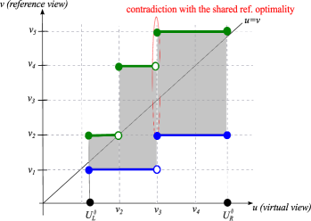
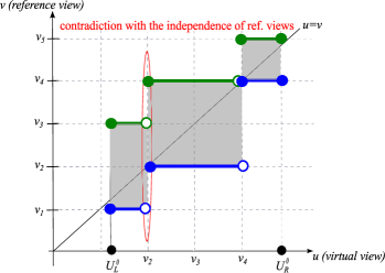
Figure 2: Reference view assignment in (a) contradicts the shared reference assumption. Reference view assignment in (b) respects the shared reference assumption but contradicts the independence of reference optimality assumption.

We can graphically illustrate possible solutions to the optimization problem (27) under the assumption of shared optimality of reference views. Fig. 2 depicts the selected reference views for virtual views in the navigation window. In the figure, the $x$-axis represents the virtual views in the window $[U_{L}^{0},U_{R}^{0}]$ that require synthesis. Correspondingly, on the $y$-axis are two piecewise constant (PWC) functions representing the left and right reference views selected for synthesis of each virtual view $u$ in the window, assuming that for each $u\in[U_{L}^{0},U_{R}^{0}]$ there must be one selected reference pair $(v_{L},v_{R})$ such that $v_{L}\leq u\leq v_{R}$. A constant line segment—e.g., $v=v_{1}$ for $U^{0}_{L}\leq u\leq v_{3}$ in Fig. 2—means that the same reference is used for a range of virtual views. This graphical representation results in two PWC functions—left and right reference views—above and below the $u=v$ line. The set of selected reference views are the unions of the constant step locations in the two PWC functions.

Under the assumption of shared reference optimality we see that the selected reference views in Fig. 2 cannot be an optimal solution. Specifically, virtual views $v_{3}-1/L$ and $v_{3}$ employ references $[v_{1},v_{4}]$ and $[v_{2},v_{5}]$ respectively. However, if references $[v_{1},v_{4}]$ are better than $[v_{2},v_{5}]$ for virtual view $v_{3}-1/L$, they should be better for virtual view $v_{3}$ also according to shared reference optimality in (29). An example of an optimal solution candidate under the assumption of shared reference optimality is shown in Fig. 2.

IV-C NP-hard Proof

We now outline a proof-by-construction that shows the reference view selection problem (27) is NP-hard under the shared optimality assumption. We show it by reducing the known NP-hard set cover (SC) problem [49] to a special case of the reference view selection problem. In SC, a set of items $\mathcal{S}$ (called the universe) are given, together with a defined collection $\mathcal{C}$ of subsets of items in $\mathcal{S}$. The SC problem is to identify at most $K$ subsets from collection $\mathcal{C}$ that covers $\mathcal{S}$, i.e., a smaller collection $\mathcal{C}^{\prime}\subseteq\mathcal{C}$ with $|\mathcal{C}^{\prime}|\leq K$ such that every item in $\mathcal{S}$ belongs to at least one subset in collection $\mathcal{C}^{\prime}$.

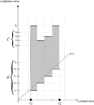
Figure 3: Example of items set $\mathcal{S}$ and collection of sets $\mathcal{C}$, with $|\mathcal{S}|=5$ and $|\mathcal{C}|=4$.

We construct a corresponding special case of our reference view selection problem as follows. For each item $i$ in $\mathcal{S}=\{1,\ldots,|\mathcal{S}|\}$ in the SC problem, we first construct an undistorted reference view $i$. In addition, we construct a default undistorted right reference view $|\mathcal{S}|+1$, and the navigation window is set to $[U^{0}_{L},U^{0}_{R}]=[1,|\mathcal{S}|+1]$ and $L=2$. Further, for each item $i$ in $\mathcal{S}$, we construct a virtual view $i+\frac{1}{2}$ that requires the selection of left reference $i$, in combination of default right reference $|\mathcal{S}|+1$, for the resulting synthesized view distortion $d_{i+\frac{1}{2}}(i,|\mathcal{S}|+1,0,0)$ to achieve distortion $\bar{D}<\infty$. Thus the selection of $|\mathcal{S}|$ left references and one default right reference $|\mathcal{S}|+1$ consumes $|\mathcal{S}|+1$ views worth of bandwidth already. See Fig. 3 for an illustration. Note that given this selection of left reference views, any selection of right reference views will satisfy the shared optimality of reference views assumption.

For each subset $j$ in collection $\mathcal{C}=\{1,\ldots,|\mathcal{C}|\}$ in the SC problem, we construct a right reference view $|\mathcal{S}|+1+j$, such that if item $i$ belongs to subset $j$ in the SC problem, the synthesized distortion $d_{i+\frac{1}{2}}(i,|\mathcal{S}|+1+j,0,0)$ at virtual view $1+\frac{1}{2}$ will be reduced to $\bar{D}-\Delta$ given right reference view $|\mathcal{S}|+1+j$ is used. The corresponding binary decision we ask is: given channel bandwidth of $|\mathcal{S}|+1+K$, is there a reference view selection such that the resulting synthesized view distortion is $|\mathcal{S}|(\bar{D}-\Delta)$ or less?

From construction, it is clear that to minimize overall distortion, left reference views $1,\ldots,|\mathcal{S}|$ and default right reference view $|\mathcal{S}|+1$ must be first selected in any solution with distortion $<\infty$. Given remaining budget of $K$ additional views, if distortion of $|\mathcal{S}|(\bar{D}-\Delta)$ is achieved, that means $K$ or fewer additional right reference views are selected to reduce synthesized distortion from $\bar{D}$ to $\bar{D}-\Delta$ at each of the virtual view $i+\frac{1}{2}$, $i\in\{1,\ldots,|\mathcal{S}|\}$. Thus these additionally $K$ or fewer selected right reference views correspond exactly to the subsets in the SC problem that covers all items in the set $\mathcal{S}$. This solving this special case of the reference view selection problem is no easier than solving the SC problem, and therefore the reference view selection problem is also NP-hard. $\Box$

V Optimal View Selection Algorithm

Given that the reference view selection problem (27) is NP-hard under the assumption of shared optimality of reference views, in this section we introduce another assumption on the synthesized view distortion that holds in most common 3D scenes. Given these two assumptions, we show that (27) can now be solved optimally in polynomial time by a DP algorithm. We also analyze the DP algorithm’s computation complexity.

V-A Independence of reference optimality assumption

The second assumption on the synthesized view distortion $d_{u}(\,)$ is the independence of reference optimality, stated formally as follows:

$$\text{if }d_{u}(v_{L},v_{R},D(v_{L}),D(v_{R}))\leq d_{u}(v_{L}^{\prime},v_{R},D(v_{L}^{\prime}),D(v_{R}))$$ (32)

$$\text{then }d_{u}(v_{L},v_{R}^{\prime},D(v_{L}),D(v_{R}^{\prime}))\leq d_{u}(v_{L}^{\prime},v_{R}^{\prime},D(v_{L}^{\prime}),D(v_{R}^{\prime}))$$

for $\max\{v_{L},v_{L}^{\prime}\}\leq u\leq\min\{v_{R},v_{R}^{\prime}\}$. In words, the assumption (32) states that if $v_{L}$ is a better left reference than $v_{L}^{\prime}$ when synthesizing virtual view $u$ using $v_{R}$ as right reference, then $v_{L}$ remains the better left reference to synthesize $u$ even if a different right reference $v_{R}^{\prime}$ is used. This assumption essentially states that contributions towards the synthesized image from the two references are independent from each other, which is reasonable since each rendered pixel in the synthesized view is typically copied from one of the two references, but not both. We can also argue for the plausibility of this assumption as a consequence of the two aforementioned functional trends in the synthesized view distortion $d_{v}(\,)$ in Section IV. Consider first the case where the reference views $v_{L},v_{R},v_{L}^{\prime},v_{R}^{\prime}$ have zero distortion. The monotonicity in predictor’s distance in (30) for a common right reference view becomes

$$|u-v_{L}|+|v_{R}-u| \leq|u-v_{L}^{\prime}|+|v_{R}-u|\hskip 14.22636pt\longrightarrow\hskip 14.22636pt|u-v_{L}|\leq|u-v_{L}^{\prime}|$$ (33)

where $\max\{v_{L},v_{L}^{\prime}\}<u<v_{R}$. Thus if $v_{L}$ is preferred to $v_{L}^{\prime}$ for $v_{R}>u$, it will hold also for $v_{R}^{\prime}$ as long as $v_{R}^{\prime}>u$. Consider now the case where the reference views $v_{L},v_{R},v_{L}^{\prime},v_{R}^{\prime}$ have non-zero distortions. Introducing the equivalent reference views $v_{L}^{\#}<v_{L}$ with no distortion $D(v_{L}^{\#})=0$, the same argument of (33) holds for the equivalent reference views, leading to $|u-v_{L}^{\#}|\leq|u-v_{L}^{\prime\#}|$, $\forall v_{R}>u$.

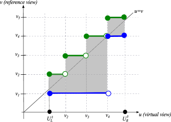
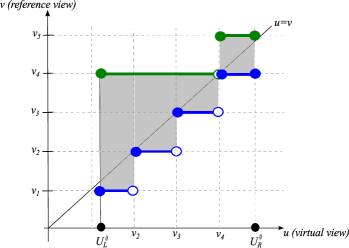
Figure 4: Reference view assignments in (a) and (b) are optimal solution candidates under both assumptions. We name these two cases “shared-left” and “shared-right”, respectively.

We illustrate different optimal solution candidates to (27) now under both virtual view distortion assumptions to impart intuition. We see that the assumption of independence of reference optimality would prevent the reference view selection in Fig. 2 from being an optimal solution. Specifically, we see that both $v_{3}$ and $v_{4}$ are feasible right reference views for virtual views $v_{2}-1/L$ and $v_{2}$. Regardless of which left references are selected for these two virtual views, if $v_{3}$ is a strictly better right reference than $v_{4}$, then having both virtual views select $v_{3}$ as right reference will result in a lower overall distortion (and vice versa). If $v_{3}$ and $v_{4}$ are equally good right reference views resulting in the same synthesized view distortion, then selecting just $v_{4}$ without $v_{3}$ can achieve the same distortion with one fewer right reference view. Thus the selected reference views in Fig. 2 cannot be optimal.

We can thus make the following observation: as virtual view $u$ increases, an optimal solution cannot switch right reference view from current $v_{R}$ earlier than $u=v_{R}$. Conversely, as virtual view $u$ decreases, an optimal solution cannot switch left reference view from current $v_{L}$ earlier than $u=v_{L}-1/L$. As examples, Fig. 4 provides solutions of left and right reference views for virtual views in the navigation window. In the figure, on the $x$-axis are the virtual views $u$ in the window $[U_{L}^{0},U_{R}^{0}]$ that require synthesis. Correspondingly, on the $y$-axis are the left and right reference views (blue and red PWC functions respectively) selected to synthesize each virtual view $u$ in the window. We see that the reference view selections in Fig. 4 and Fig. 4 are optimal solution candidates to (27). Thus, the optimal reference view selections must be graphically composed of “staircase” virtual view ranges as shown in Fig. 4 and Fig. 4. In other words, either a shared left reference view $v^{s}_{L}$ is used for multiple virtual view ranges $[u_{i},u_{i+1})$ where each range has the same $v^{s}_{L}$ as left reference (“shared-left” case), or a shared right reference view $v^{s}_{R}$ is used for multiple ranges $[u_{i},u_{i+1})$, where each range has $v^{s}_{R}$ as its right reference (“shared-right” case). This motivates us to design an efficient DP algorithm to solve (27) optimally in polynomial time.

V-B DP Algorithm

We first define a recursive function $\Phi(u_{L},v_{L},k)$ as the minimum aggregate synthesized view distortion of views between $u_{L}$ and $U_{R}^{0}$, given $v_{L}$ is the selected left reference view for synthesizing view $u_{L}$, and there is a budget of $k$ additional reference views. To analyse $\Phi(u_{L},v_{L},k)$, we consider the two “staircase” cases identified by Fig. 4 and Fig. 4 separately, and show how $\Phi(u_{L},v_{L},k)$ can be evaluated in each of the cases.

Consider first the “shared-left” case (Fig. 4) where a shared left reference view is employed in a sequence of virtual view ranges. A view range represents a contiguous range of virtual viewpoints that employ the same left and right reference views. The algorithm selects a new right reference view $v$, $v>u_{L}$, creating a new range of virtual views $[u_{L},v)$. Virtual views in range $[u_{L},v)$ are synthesized using a shared left reference $v_{L}$ and the newly selected reference view $v$, resulting in distortion $d_{u}(v_{L},v,D(v_{L}),D(v))$ for each virtual view $u$, $u_{L}\leq u<v$. The aggregate distortion function $\Phi(u_{L},v_{L},k)$ for this case is the distortion of views in $[u_{L},v)$ plus a recursive term $\Phi(v,\Lambda(v_{L},v),k-1)$ to account for aggregate synthesized view distortions to the right of $v$:

$$\sum_{u=u_{L}}^{v-\frac{1}{L}}d_{u}(v_{L},v,D(v_{L}),D(v))+\Phi(v,\Lambda(v_{L},v),k-1)$$ (34)

where $k-1$ is the remaining budget of additional reference views, and $\Lambda(v_{1},v_{2})$ chooses the better of the two left reference views, $v_{1}$ and $v_{2}$, for the recursive function $\Phi(\,)$. In particular, using any right reference view $v_{R}$ and virtual view $u$, where $\max\{v_{1},v_{2}\}<u<v_{R}$, we set $\Lambda(v_{1},v_{2})=v_{1}$ if virtual view $u$ is better synthesized using $v_{1}$ as left reference than $v_{2}$ (and set $\Lambda(v_{1},v_{2})=v_{2}$ otherwise). Formally, the left reference selection function $\Lambda(v_{1},v_{2})$ is defined as:

$$\Lambda(v_{1},v_{2})=\left\{\begin{array}[]{ll}v_{1}&\mbox{if}~{}~{}d_{u}(v_{1},v_{R},D(v_{l}),D(v_{R}))\leq d_{u}(v_{2},v_{R},D(v_{2}),D(v_{R}))\\ v_{2}&\mbox{o.w.}\end{array}\right.$$ (35)

Given our two assumptions, we know that the selected left reference $\Lambda(v_{1},v_{2})$ remains better for all other virtual views $u$ in $[\max\{v_{1},v_{2}\},v_{R}]$.

We now consider the “shared-right” case (Fig. 4) where a newly selected view $v$ is actually a common right reference view for a sequence of virtual view ranges from $u_{L}$ to $v$. We first define a companion recursive function $\Psi(u_{L},v_{L},v_{R},n)$ that returns the minimum aggregate synthesized view distortion from view $u_{L}$ to $v_{R}$, given that $v_{L}$ is the selected left reference view, $v_{R}$ is the common right reference view, and there is a budget of $n$ other left reference views in addition to $v_{L}$. We can write $\Psi(u_{L},v_{L},v_{R},n)$ recursively as follows:

$$\Psi(u_{L},v_{L},v_{R},n)=\left\{\begin{array}[]{ll}\min\limits_{v>u_{L}}\sum\limits_{u=v_{L}}^{v-\frac{1}{L}}d_{u}(v_{L},v_{R},D(v_{L}),D(v_{R}))+\Psi(v,v,v_{R},n-1)&\mbox{if}~{}~{}k\geq 1\\ \sum\limits_{u=v_{L}}^{v_{R}-\frac{1}{L}}d_{u}(v_{L},v_{R},D(v_{L}),D(v_{R}))&\mbox{o.w.}\end{array}\right.$$ (36)

In more details, the equation (36) states that $\Psi(u_{L},v_{L},v_{R},n)$ is the synthesized view distortion of views in the range $[u_{L},v)$, plus the recursive distortion $\Psi(v,v,v_{R},n-1)$ from view $v$ to $v_{R}$ with a reduced reference view budget $n-1$.

We can now put the two cases together into a complete definition of $\Phi(u_{L},v_{L},k)$ as follows:

$$\Phi(u_{L},v_{L},k) =\min_{v>v_{L}}\left\{\min\left[\underbrace{\sum_{u=u_{L}}^{v-\frac{1}{L}}d_{u}(v_{L},v,D(v_{L}),D(v))+\Phi(v,\Lambda(v_{L},v),k-1)}_{\text{``shared-left" case }},\right.\right.$$ (37)

$$\hskip 56.9055pt\left.\left.\underbrace{\min_{1\leq n\leq k-1}\Psi(u_{L},v_{L},v,n)+\Phi(v,v,k-n-1)}_{\text{``shared-right" case }}\right]\right\}$$

The relation (37) states that $\Phi(u_{L},v_{L},k)$ examines each candidate reference view $v$, $v>v_{L}$, which can be used either as right reference for synthesizing virtual views in $[u_{L},v)$ with left reference $v_{L}$ (“shared-left” case), or as a common right reference for a sequence of $n+1$ virtual view ranges within the interval $[u_{L},v)$ (“shared-right” case).

When the remaining view budget is $k=1$, the relation in (37) $\Phi(u_{L},v_{L},1)$ simply selects a right reference view $v$, $v\geq U_{R}^{0}$, which minimizes the aggregate synthesized view distortion for the range $[u_{L},U_{R}^{0}]$:

$$\Phi(u_{L},v_{L},1)=\min_{v\geq U_{R}^{0}}\sum_{u=u_{L}}^{U_{R}^{0}}d_{u}(v_{L},v,D(v_{L}),D(v))$$ (38)

Having defined $\Phi(u_{L},v_{L},k)$, we can identify the best $K$ reference views by calling $\Phi(U_{L}^{0},v,K)$ repeatedly to identify the best leftmost reference view $v$, $v\leq U_{L}^{0}$, and start the selection of the $K-1$ remaining reference views as follows

$$\min_{v\leq U_{L}^{0}}\Phi(U_{L}^{0},v,K-1)$$ (39)

V-C Computation Complexity

Our proposed DP algorithm requires two different tables to be stored. The first time $\Psi(u_{L},v_{L},v_{R},n)$ is computed, the result can be stored in entry $[(u_{L}-U_{L}^{0})/L][(v_{L}-U_{L}^{0})/L][(v_{R}-U_{L}^{0})/L][n]$ of a DP table ${\boldsymbol{\Psi}}^{*}$, so that subsequent calls with the same arguments can be simply looked up. Analogously, the first time $\Phi(u_{L},v_{L},k)$ is called, the computed value is stored in entry $[(u_{L}-U_{L}^{0})/L][(v_{L}-U_{L}^{0})/L][k]$ of another DP table ${\boldsymbol{\Phi}}^{*}$ to avoid repeated computation in future recursive calls.

We bound the computation complexity of our proposed algorithm (37) by computing a bound on the sizes of the required DP tables and the cost in computing each table entry. For notation convenience, let the number of reference views and synthesized views be $S_{v}=(V-1)/L$ and $S_{u}=(U_{R}^{0}-U_{L}^{0})/L$, respectively. The size of DP table ${\boldsymbol{\Phi}}^{*}$ is no larger than $S_{u}\times S_{v}\times K$. The cost of computing an entry in ${\boldsymbol{\Phi}}^{*}$ using (37) over all possible reference views $v$ involves the computation of the “shared-left” case with complexity $O(S_{u})$ and the one of the “shared-right” case with complexity $O(K)$. Thus, each table entry has complexity $O(S_{v}S_{u}+S_{v}K)$. Hence the complexity of completing the DP table ${\boldsymbol{\Phi}}^{*}$ is $O(S_{u}^{2}S_{v}^{2}K+S_{u}S_{v}^{2}K^{2})$. Given that in typical setting $S_{u}\gg K$, the complexity for computing DT table ${\boldsymbol{\Phi}}^{*}$ is thus $O(S_{u}^{2}S_{v}^{2}K)$.

We can perform similar procedure to estimate the complexity in computing DP table ${\boldsymbol{\Psi}}^{*}$. The size of the table in this case is upper-bounded by $S_{u}\times S_{v}\times S_{v}\times K$. The complexity in computing each entry is $O(S_{u})$. Thus the complexity of computing DP table ${\boldsymbol{\Psi}}^{*}$ is $O(S_{u}^{2}S_{v}^{2}K)$. which is the same as DP table ${\boldsymbol{\Phi}}^{*}$. Thus the overall computation complexity of our solution in (37) is also $O(S_{u}^{2}S_{v}^{2}K)$.

VI Simulation Results

TABLE I: Viewpoints notation.

Camera ID as in [50], “Statue”	${50}$	$51$	$52$	$53$	$54$	$55$	$56$	$57$	${58}$	$59$	$\ldots$	${98}$
Camera ID as in [50], “Mansion”	${25}$	$26$	$27$	$28$	$29$	$30$	$31$	$32$	${33}$	$34$	$\ldots$	${73}$
Camera ID in our work	${0}$	$1.125$	$1.25$	$1.375$	$1.5$	$1.625$	$1.75$	$1.875$	${1}$	$2.125$	$\ldots$	${6}$

VI-A Settings

We study the performance of our algorithm and we show the distortion gains offered by cloudlets-based virtual view synthesis. For a given navigation window $[U_{L}^{0},U_{R}^{0}]$, we provide the average quality at which viewpoints in the navigation window is synthesized. This means that we evaluate the average distortion of the navigation window as $(1/N)\sum_{u=U_{L}^{0}}^{U_{R}^{0}}d_{u}$, with $N$ being the number of synthesized viewpoints in the navigation window, and we then compute the corresponding PSNR. In our algorithm, we have considered the following model for the distortion of the synthesized viewpoint $u$ from reference views $V_{L}$, $V_{R}$

$$d_{u}(V_{L},V_{R},D_{L},D_{R})=\alpha D_{min}+(1-\alpha)\beta D_{max}+\left[1-\alpha-(1-\alpha)\beta\right]D_{I}$$ (40)

where $D_{min}=\min\{D_{L},D_{R}\}$, $D_{max}=\max\{D_{L},D_{R}\}$, $D_{I}$ is the inpainted distortion, and $\alpha=\exp\left(-\gamma|u-V_{min}|d\right),\,\beta=\exp\left(-\gamma|u-V_{max}|d\right)$ with $d$ is the distance between two consecutive camera views $v_{i}$ and $v_{i}+1$, $V_{min}=V_{L}$ if $D_{L}\leq D_{R}$, $V_{min}=V_{R}$ otherwise, and $V_{max}=V_{L}$ if $D_{L}>D_{R}$, $V_{max}=V_{R}$. The model can be explained as follows. A virtual synthesis $u$, when reconstructed from $(V_{L},V_{R})$ has a relative portion $\alpha\in[0,1]$ that is reconstructed at a distortion $D_{min}$, from the dominant reference view, defined as the one with minimum distortion. The remaining portion of the image, i.e., $1-\alpha$, is either reconstructed by the non-dominant reference view for a potion $\beta$, at a distortion $D_{max}$, or it is inpainted, at a distortion $D_{I}$.

The results have been carried out using 3D sequences “Statue” and “Mansion” [50], where $51$ cameras acquire the scene with uniform spacing between the camera positions. The spacing between camera positions is $5.33$ mm and $10$ mm for “Statue” and “Mansion”, respectively. Among all camera views provided for both sequences, only a subset represents the set of camera views $\mathcal{V}$ available at the cloudlet, while the remaining are virtual views to be synthesized. Table I depicts how the camera notation used in [50] is adapted to our notation. Finally, for the “Mansion” sequence, in the theoretical model in (40) we used $\beta=0.2$, $D_{max}=450$, and $d=50$, while for the “Statue” sequence we used $\beta=0.2$, $D_{max}=100$, and $d=25$.

In the following, we compare the performance achieved by virtual view synthesis in the cloudlets with respect to the scenario in which cloudlets only send to users a subset of camera views. We denote by $\mathcal{T}_{s}$ the subset of selected reference views when synthesis is allowed in the network, and by $\mathcal{T}_{ns}$ the subset of selected reference views when only camera views can be sent as reference views, i.e., when synthesis is not allowed in the network. For both the cases of network synthesis and no network synthesis, the best subset of reference views is evaluated both with the proposed view selection algorithm and with an exact solution, i.e., an exhaustive search of all possible combinations of reference views. For the proposed algorithm, the distortion is evaluated both with experimental computation of the distortion, where the results are labeled “Proposed Alg. (Experimental Dist)”, and with the model in (40), results labeled “Proposed Alg. (Theoretical Dist)”. For all three algorithms, once the optimal subset of reference view is selected, the full navigation window is reconstructed experimentally and the mean PSNR of the actual reconstructed sequence is computed.

In the following, we first validate the distortion model in (40) as well as the proposed optimization algorithm. Then, we provide simulation using the model in (40) and study the gain offered by network synthesis. For the sake of clarity in the notation, in the following we identify the viewpoints by their indexes only. This means that the set of camera views $\{v_{0},v_{1},v_{3}\}$, for example, is denoted in the following by $\{0,1,3\}$. Analogously for the navigation window $[u_{0.75},u_{5.25}]$ is denoted in the following by $[{0.75},{5.25}]$.

VI-B Performance of the view selection algorithm

In Fig. 5, we provide the mean PSNR as a function of the available bandwidth $C$ in the setting of a regular spaced cameras set $\mathcal{V}=\{0,1,2,\ldots,5,6\}$, and a navigation window $[{0.75},{5.25}]$ requested by the user. Results are provided for the “Mansion” and the “Statue” sequences in Fig. 5(a) and Fig. 5(b), respectively. For the “Mansion” sequence, the proposed algorithm with experimental distortion perfectly matches the exhaustive search. Also the proposed algorithm based on theoretical distortion nicely matches the exhaustive search method, with the exception of the experimental point at $C=4$ in the network synthesis case. In that experiment, the algorithm selects as best subset $\mathcal{T}_{s}=\{{0.75},2,4,{5.25}\}$ rather than $\mathcal{T}_{s}=\{{0.75},2,3,{5.25}\}$ selected by the exhaustive search. Beyond the good match between exhaustive search and proposed algorithm, Fig. 5(a) also shows the gain achieved in synthesizing reference views at the cloudlets. For $C=2$, the optimal sets of reference views are $\mathcal{T}_{s}=\{{0.75},{5.25}\}$ and $\mathcal{T}_{ns}=\{0,6\}$. The possibility of selecting the view at position $0.75$ as reference view reduced the reference view distance for viewpoints in $[{0.75},{5.25}]$ compared to the case in which camera view $0$ is selected. Thus, as long as the viewpoint ${0.75}$ is synthesized at a good quality in the network, synthesizing in the network improves the quality of the reconstructed region of interest, when the bandwidth $C$ is limited. Increasing the channel capacity reduces the quality gain between synthesis and no synthesis at the cloudlets. For $C=4$, for example, the virtual viewpoint $0.75$ is used to reconstruct the views range $[0.75,2)$ of the navigation window. Thus, the benefit of selecting $0.75$ rather than $0$ is limited to a portion of the navigation window and this portion usually decreases for large $C$. Similar considerations can be derived from Fig. 5(b), for the “Statue” sequence. We observe a very good match between the proposed algorithm and the exhaustive search one.

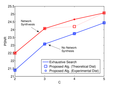
(a) Mansion

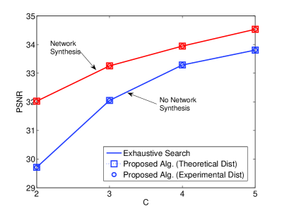
(b) Statue

Figure 5: Validation of the proposed optimization model with equally spaced cameras set $\mathcal{V}=\{0,1,2,\ldots,5,6\}$, and a navigation window $[0.75,5.25]$ for “Mansion” and “Statue” sequences.

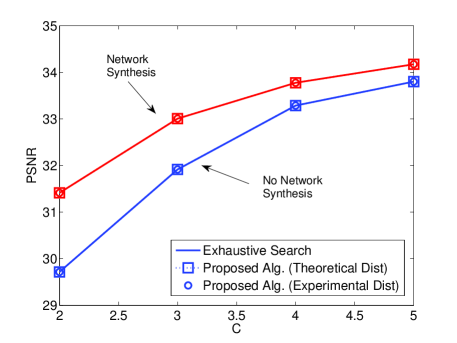
Figure 6: Validation of the proposed optimization model for “Statue” sequence with unequally spaced cameras $\mathcal{V}=\{0,1.5,2,2.75,4,5,6\}$ and a navigation window $[0.75,5.25]$.

We then compare in Fig. 6 the performance of the exhaustive search algorithm with our optimization method in the case of non-equally spaced cameras. The “Statue” sequence is considered with unequally spaced cameras set $\mathcal{V}=\{0,1.5,2,2.75,4,5,6\}$, and a navigation window $[0.75,5.25]$ at the client. Similarly to the equally spaced scenario, the performance of proposed optimization algorithm matches the one of the exhaustive search. This confirms the validity of our assumptions and the optimality of the DP optimization solution. Also in this case, a quality gain is offered by virtual view synthesis in the network, with a maximum gain achieved for $C=2$, with optimal reference views $\mathcal{T}_{s}=\{0.75,5.25\}$ and $\mathcal{T}_{ns}=\{0,6\}$.

VI-C Network synthesis gain

Now, we aim at studying the performance gain due to synthesis in the network for different scenarios. However, multiview video sequences (with both texture and depth maps) currently available as test sequences have a very limited number of views (e.g., $8$ views in the Ballet video sequences). Because of the lack of test sequences, we consider synthetic scenarios and we adopt the distortion model in (40) both for solving the optimization algorithm and evaluating the system performance. The following results are meaningful since we already validated our synthetic distortion model in the previous subsection.

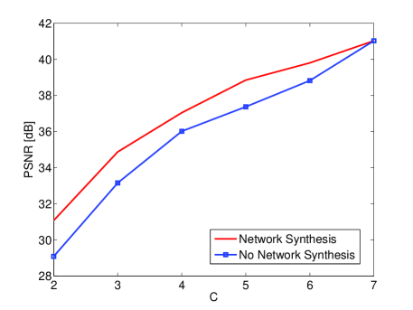
Figure 7: PSNR (in dB) as a function of the channel capacity $C$ for different channel capacity values $C$ for a regular spaced camera set with varying distance among cameras, $\gamma=0.3$, $D_{I}=300$, navigation window $[0.75,5.25]$, and camera set $\mathcal{V}=\{0,1,2,\ldots,5,6\}$ (equally spaced cameras).

TABLE II: Optimal subsets for the scenario of Fig. 7.

$C$	$\mathcal{T}_{s}$	$\mathcal{T}_{ns}$
$2$	$\{0.75,5.25\}$	$\{\boldsymbol{0},\boldsymbol{6}\}$
$3$	$\{0.75,\boldsymbol{3},5.25\}$	$\{\boldsymbol{0},\boldsymbol{3},\boldsymbol{6}\}$
$4$	$\{0.75,\boldsymbol{2},\boldsymbol{4},5.25\}$	$\{\boldsymbol{0},\boldsymbol{2},\boldsymbol{4},\boldsymbol{6}\}$
$5$	$\{0.75,\boldsymbol{2},\boldsymbol{3},\boldsymbol{4},5.25\}$	$\{\boldsymbol{0},\boldsymbol{2},\boldsymbol{3},\boldsymbol{4},\boldsymbol{6}\}$
$6$	$\{\boldsymbol{0},\boldsymbol{1},\boldsymbol{2},\boldsymbol{3},\boldsymbol{4},5.25\}$	$\{\boldsymbol{0},\boldsymbol{1},\boldsymbol{2},\boldsymbol{3},\boldsymbol{4},\boldsymbol{6}\}$
$7$	$\{\boldsymbol{0},\boldsymbol{1},\boldsymbol{2},\boldsymbol{3},\boldsymbol{4},\boldsymbol{5},\boldsymbol{6}\}$	$\{\boldsymbol{0},\boldsymbol{1},\boldsymbol{2},\boldsymbol{3},\boldsymbol{4},\boldsymbol{5},\boldsymbol{6}\}$

TABLE III: Selected subset of reference views and associated quality for scenarios with $[U_{L}^{0},U_{R}^{0}]=[0.75,7.25]$ , $d=25$ mm, $\gamma=0.2$, $D_{max}=200$.

$\mathcal{V}=\{0,1,3,5,7,8\}$, case $a)$					$\mathcal{V}=\{0,2,3,4,7,8\}$, case $b)$
$C$	$\mathcal{T}_{s}$	PSNR	$\mathcal{T}_{ns}$	PSNR	$C$	$\mathcal{T}_{s}$	PSNR	$\mathcal{T}_{ns}$	PSNR
$2$	$\{0.75,7.25\}$	29.39	$\{\boldsymbol{0},\boldsymbol{8}\}$	28.04	$2$	$\{0.75,7.25\}$	29.08	$\{\boldsymbol{0},\boldsymbol{8}\}$	28.04
$3$	$\{0.75,\boldsymbol{3},7.25\}$	32.35	$\{\boldsymbol{0},\boldsymbol{3},\boldsymbol{8}\}$	31.13	$3$	$\{0.75,\boldsymbol{4},7.25\}$	32.33	$\{\boldsymbol{0},\boldsymbol{4},\boldsymbol{8}\}$	31.49
$4$	$\{0.75,\boldsymbol{3},\boldsymbol{5},7.25\}$	35.24	$\{\boldsymbol{0},\boldsymbol{3},\boldsymbol{5},\boldsymbol{8}\}$	33.87	$4$	$\{\boldsymbol{0},\boldsymbol{2},\boldsymbol{4},7.25\}$	34.18	$\{\boldsymbol{0},\boldsymbol{2},\boldsymbol{4},\boldsymbol{8}\}$	33.21
$5$	$\{\boldsymbol{0},\boldsymbol{1},\boldsymbol{3},\boldsymbol{5},7.25\}$	35.85	$\{\boldsymbol{0},\boldsymbol{1},\boldsymbol{3},\boldsymbol{5},\boldsymbol{8}\}$	35.017	$5$	$\{\boldsymbol{0},\boldsymbol{2},\boldsymbol{4},\boldsymbol{7},\boldsymbol{8}\}$	34.92	$\{\boldsymbol{0},\boldsymbol{2},\boldsymbol{4},\boldsymbol{7},\boldsymbol{8}\}$	34.92
$6$	$\{\boldsymbol{0},\boldsymbol{1},\boldsymbol{3},\boldsymbol{5},\boldsymbol{7},\boldsymbol{8}\}$	36.56	$\{\boldsymbol{0},\boldsymbol{8}\}$	36.56	$6$	$\{\boldsymbol{0},\boldsymbol{2},\boldsymbol{3},\boldsymbol{4},\boldsymbol{7},\boldsymbol{8}\}$	35.60	$\{\boldsymbol{0},\boldsymbol{2},\boldsymbol{4},\boldsymbol{7},\boldsymbol{8}\}$	35.60

We consider the cases of equally spaced cameras $\left(\mathcal{V}=\{0,1,2,\ldots,5,6\}\right)$ and unequally spaced cameras $\left(\mathcal{V}=\{0,1,3,5,7,8\}\right.$ and $\left.\mathcal{V}=\{0,2,3,4,7,8\}\right)$ capturing the scene of interest. In Fig. 7, we show the mean PSNR as a function of the available channel capacity $C$ when the navigation window requested by the user is $[0.75,5.25]$ and cameras are equally spaced. The distortion of the synthesized viewpoints is evaluated with (40), with $\gamma=0.2$, $D_{I}=200$, and $d=25$. The case of synthesis in the network is compared with the one in which only camera views can be sent to clients. In Table II, we show the optimal subsets $\mathcal{T}_{s}$ and $\mathcal{T}_{ns}$ associated to each simulation point in Fig. 7, where camera views indexes are highlighted in bold. We observe that the case with synthesis in the network performs best in terms of quality over the navigation window. When $C=2$, $\mathcal{T}_{s}:\{0.75,5.25\}$ for the network synthesis case, and $\mathcal{T}_{ns}:\{0,6\}$, otherwise. However, the larger the channel capacity the less the need for sending virtual viewpoints. When $C=6$, for example, both camera views $0$ and $1$ can be sent, thus there is no gain in transmitting only view $0.75$. Finally, when $C=7$ and all camera views can be sent to clients, $\mathcal{T}_{s}=\mathcal{T}_{ns}=\mathcal{V}$, with $\mathcal{V}$ being the set of camera views. As expected, sending synthesized viewpoints as reference views leads to a quality gain only in constrained scenarios in which the channel capacity does not allow to send all views required for reconstructing the navigation window of interest.

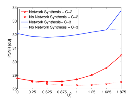
Figure 8: PSNR (in dB) vs. $U_{L}^{0}$ for a camera set $\mathcal{V}=\{0,2,3,4\}$, navigation window $[U_{L}^{0},4]$, with $d=50$, $\gamma=0.2$, and $D_{I}=200$.

We now study the gain in allowing network synthesis when camera views are not equally spaced. In Table III, we provide the optimal subsets of reference views for both sets of unequally spaced cameras $\left(\mathcal{V}=\{0,1,3,5,7,8\}\right.$ and $\left.\mathcal{V}=\{0,2,3,4,7,8\}\right)$. Similarly to the case of equally spaced cameras, we observe that virtual viewpoints are selected as reference views (i.e., they are in the best subset $\mathcal{T}_{s}$) when the bandwidth $C$ is limited. For the camera set $a)$ the virtual view $0.75$ is selected as reference view also for $C=4$, while the camera set $b)$ prefers to select the camera views $0$, $2$ at $C=4$. This is justified by the fact that in the latter scenario, the viewpoint $0.75$ is synthesized from $(V_{L},V_{R})=(0,2)$ thus at a larger distortion than the viewpoint $0.75$ in scenario $a)$, where the viewpoint is synthesized from $(V_{L},V_{R})=(0,1)$. This distortion penalty makes the synthesis worthy when the channel bandwidth is highly constrained ($C=2,3$), but not in the other cases.

In Fig. 8, the average quality of the client navigation is provided as a function of the left extreme view $U_{L}^{0}$ of the navigation window $[U_{L}^{0},4]$ with the camera set $\mathcal{V}=\{0,2,3,4\}$ with $d=50$, $\gamma=0.2$, and $D_{I}=200$ in (40). It is worth noting that $U_{L}^{0}$ ranges from $0$ to $1.875$ and only view $0$ is a camera view in this range. When $U_{L}^{0}=0$ and $C=2$, the reference views $0$ and $4$ perfectly cover the entire navigation window requested by the user, so there is no need for sending any virtual viewpoint as reference view. This is no more true for $U_{L}^{0}>0$. When the channel capacity is $C=2$, the gain in allowing synthesis at the cloudlets increases with $U_{L}^{0}$. This is justified by the fact that in a very challenging scenario (i.e., limited channel capacity), the larger $U_{L}^{0}$ the less efficient is it is to send the reference view $0$ to reconstruct images in $[U_{L}^{0},4]$. At the same time, sending $2$ and $4$ as reference views would not allow to reconstruct the viewpoints lower than $2$. This gain in allowing network synthesis is reflected in the PSNR curves of Fig. 8, where we can observe an increasing gap between the case of synthesis allowed and not allowed for $C=2$. This gap is however reduced for the scenario of $C=3$. This is expected since the navigation window is a limited one, at most ranging from $0$ to $4$ and $3$ reference views cover the navigation window pretty well.

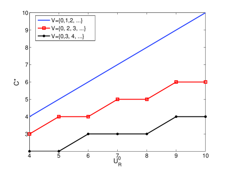
Figure 9: Thresholding $C$ vs. $U_{R}^{0}$ for a navigation window $[0.5,U_{R}^{0}]$, with $d=50$mm, $\gamma=0.2$, and $D_{I}=200$.

To better show this tradeoff between distortion of the virtual reference view and the bandwidth gain, we introduce the thresholding channel value, denoted by $C^{\star}$. The latter is defined as the value of channel bandwidth beyond which no gain is experienced in allowing synthesis in the network compared to a case of no synthesis. In Fig. 9, we provide the behavior of the thresholding channel value as a function the navigation window, for different cameras set. In particular, we consider $U_{L}^{0}=0.5$ and we let $U_{R}^{0}$ varies from $5$ to $10$. Also, we simulate three different scenarios that differ for the available camera set. In particular, we have $\mathcal{V}=\{0,1,2,3,\ldots\}$, $\mathcal{V}=\{0,2,3,4,\ldots\}$, and $\mathcal{V}=\{0,3,4,5,\ldots\}$. The main difference is then in the reference views that can be used to synthesize the virtual viewpoint $0.5$. In the first case, $0.5$ is reconstructed from camera views $(0,1)$ while in the last case from $(0,3)$ increasing then the distortion of the synthesis. Because of this increased distortion of $0.5$, the virtual viewpoint is not always sent as reference view. In particular, we can observe that the larger the distortion of the virtual viewpoint, the lower the thresholding channel value. This means that even in challenging scenarios, as for example in the case of $U_{R}^{0}=7$ and $C=3$, if $\mathcal{V}=\{0,3,4,5,\ldots\}$ then there is no gain in synthesize in the network, while we still have a gain if $\mathcal{V}=\{0,1,2,3,\ldots\}$.

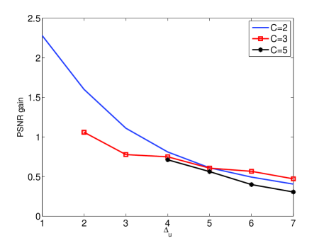
Figure 10: PSNR gain (in dB) vs. the navigation window size $\Delta_{u}$, for different channel capacity constraints $C$ when $d=50$mm, $\gamma=0.2$, and $D_{I}=200$.

In Fig. 10, we provide the mean PSNR as a function of the size of the navigation window, namely $\Delta_{u}$. More in details, for each value of $\Delta_{u}$, we define the navigation window as $[U_{L}^{0},U_{L}^{0}+\Delta_{u}]$. The starting viewpoint $U_{L}^{0}$ is randomly selected. For each realization of the navigation window, the best subset is evaluated (both when synthesis is allowed and when it is not) and the quality of the reconstructed viewpoint in the navigation window is evaluated. For each $\Delta_{u}$, we average the quality simulating all possible $U_{L}^{0}$ starting viewpoint within a total range of $[0,12]$. In the results we provide the PSNR gain, defined as the difference between the mean PSNR (in dB) when the synthesis is allowed and the mean PSNR (in dB) when only camera views are considered as reference views. Thus, the figure shows the gain in synthesizing for different sizes of the navigation window. As general trend, we observe that the quality gain decreases with $\Delta_{u}$. This is due to the fact that the gain mainly comes from the lateral reference views, that are usually virtual viewpoints if synthesis is allowed. This leads to a gain that is however reduced for large sizes of the navigation window. Finally, we also observe that the gain does not necessarily depends on the channel constraint $C$.

We now consider a scenario in which the camera views position is not a priori given. In Fig. 11, we provide the mean PSNR as a function of the variance $\sigma_{v}^{2}$, which defines the randomness of the camera views positions when acquiring the scene. More in details, we consider a navigation window $[U_{L}^{0},U_{R}^{0}]=[2,6]$. We then define a deterministic camera views set $\mathcal{V}_{D}=\{0,1,2,\ldots,6,7\}$, which is the best camera view set since it is aligned with the requested viewpoint navigation window. For each value of $\sigma_{v}^{2}$, we generate a random cameras set $\mathcal{V}$ as $\mathcal{V}=\mathcal{V}_{D}+[n_{0},n_{1},\ldots,n_{7}]$, where each $n_{i}$ is a gaussian random variable with zero mean and variance $\sigma_{v}^{2}$ with $n_{i}$ and $n_{j}$ mutually independent for $i\neq j$. Thus, the larger $\sigma_{v}^{2}$, the larger the probability for the camera view set to be not aligned with the navigation window. For each realization of $\mathcal{V}$, we run our optimization for both the cases of allowed and not allowed synthesis and we evaluate the experienced quality. For each $\sigma_{v}^{2}$ value we simulate $400$ runs and we provide in Fig. 11 the averaged quality. What it is interesting to observe is that even if camera views are not perfectly aligned with the navigation window of interest (i.e., even for large variance values) the quality degradation with respect to the case of $\sigma_{v}^{2}=0$ is limited, about $0.5$ dB for $C=3$, when network synthesis is allowed. On the contrary, when synthesis is not allowed in the cloudlet, the quality substantially decreases with $\sigma_{v}^{2}$, experiencing a PSNR loss of almost $1.5$dB. This means that network synthesis can compensate for cameras not ideally positioned in the 3D scene, as in the case of user generated content systems.

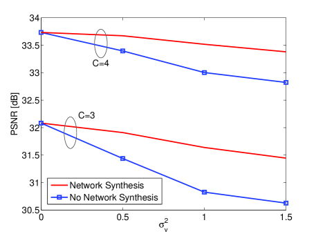
Figure 11: PSNR (in dB) vs. $\sigma_{v}^{2}$, for different channel capacity constraints $C$ when $d=50$, $\gamma=0.2$, and $D_{I}=200$.

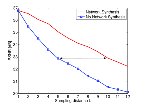
Figure 12: PSNR (in dB) vs. the sampling distance $L$, for $C=2$, $d=50$, $\gamma=0.2$, and $D_{I}=200$.

Finally, we study performance of the cloudlet-based view synthesis for a varying number of acquiring cameras. In particular, given the set of equally spaced viewpoints $\mathcal{U}$, we assume that one every $L$ viewpoints in $\mathcal{U}$ is a camera view, i.e., there are $L-1$ virtual viewpoints between consecutive camerasview. Being the viewpoints in $\mathcal{U}$ equally spaced, say at distance $d$, $Ld$ is the distance between consecutive cameras. In the following, we provide the quality behavior for $L$ ranging from $1$ to $12$. For each value of the sampling distance $L$, we simulate a navigation window spanning a range of $20d$. The navigation window is selected uniformly at random and the optimization algorithm evaluates the best subset of reference views. The experienced quality is averaged over $400$ runs and evaluated for different values of $L$. In Fig. 12, we show the mean quality for the navigation as a function of the sampling distance $L$, for the scenario with for $C=2$, $d=50$, $\gamma=0.2$, and $D_{I}=200$ in (40). It is worth noting that for a user to navigate at given quality, a much higher value of sampling distance $L$ can be used when network synthesis is allowed, with respect to the value of $L$ required with no network synthesis. For example, a mean quality in the navigation of $33$ dB is achieved with $L=5$ when network synthesis is not allowed as opposed to $L=10$ when allowing network synthesis. This means that when synthesis is allowed, half of the number of camera views can be used respect to the case in which no synthesis is allowed. Thus, view synthesis in the network allows to maintain a good navigation quality when reducing the number of cameras.

VII Conclusion

When interactive multiview video systems face limited bandwidth constraints, we argue that synthesizing reference views in the cloud improve the quality of navigation at the client side. In particular, we propose a synthesized reference view selection optimization problem aimed at finding the best subset of viewpoints to be transmitted to the decoder as reference views. This subset is not limited to captured camera views as in previous approaches but it can also include virtual viewpoints. The problem is formalized as a combinatorial optimization problem, which is shown to be NP-hard. However, we show that, under the general assumption that the distortion of synthesized viewpoints is well-behaved, the problem can be solved in polynomial time via a dynamic programming algorithm. Simulation results validate the performance gain of the proposed method and show that synthesizing reference views can improve image quality at the client by up to $2.1$dB in PSNR. We finally demonstrate that view synthesis in the network obviates to non optimal camera sampling and permits to increase the distance between camera views without affecting the quality of the navigation.

References

- [1] M. Tanimoto, M. P. Tehrani, T. Fujii, and T. Yendo, “Free-viewpoint TV,” in IEEE Signal Processing Magazine, January 2011, vol. 28, no.1.
- [2] C. Fehn, “Depth-image-based rendering (DIBR), compression and transmission for a new approach on 3D-TV,” Proc. SPIE, vol. 5291, pp. 93–104, 2004.
- [3] G. Cheung, A. Ortega, and N.-M. Cheung, “Interactive streaming of stored multiview video using redundant frame structures,” IEEE Trans. Image Processing, vol. 20, no. 3, pp. 744–761, March 2011.
- [4] Y. Liu, Q. Huang, S. Ma, D. Zhao, and W. Gao, “RD-optimized interactive streaming of multiview video with multiple encodings,” Journal of Visual Commun. and Image Representation, vol. 21, no. 5, pp. 523 – 532, March 2010.
- [5] J. Chakareski, V. Velisavljevic, and V. Stankovic, “User-action-driven view and rate scalable multiview video coding,” IEEE Trans. Image Processing, vol. 22, no. 9, pp. 3473–3484, Sept 2013.
- [6] L. Toni, T. Maugey, and P. Frossard, “Correlation-aware packet scheduling in multi-camera networks,” IEEE Trans. Multimedia, vol. 16, no. 2, pp. 496–509, Feb 2014.
- [7] T. Verbelen, P. Simoens, F. De Turck, and B. Dhoedt, “Cloudlets: Bringing the cloud to the mobile user,” in Proc. ACM Workshop on Mobile Cloud Computing and Services, 2012, pp. 29–36.
- [8] Mahadev S., P. Bahl, R Caceres, and N. Davies, “The case for vm-based cloudlets in mobile computing,” IEEE Pervasive Computing, vol. 8, no. 4, pp. 14–23, Oct 2009.
- [9] P. Merkle, A. Smolic, K. Muller, and T. Wiegand, “Efficient prediction structures for multiview video coding,” IEEE Trans. Circuits Syst. Video Technol., vol. 17, no. 11, pp. 1461–1473, Nov 2007.
- [10] J. Salvador and J.R. Casas, “Multi-view video representation based on fast monte carlo surface reconstruction,” IEEE Trans. Image Processing, vol. 22, no. 9, pp. 3342–3352, Sept 2013.
- [11] T. Maugey, A. Ortega, and P. Frossard, “Graph-based representation for multiview image geometry,” IEEE Trans. Image Processing, vol. 24, no. 5, pp. 1573–1586, May 2015.
- [12] T. Fujihashi, Ziyuan Pan, and T. Watanabe, “UMSM: A traffic reduction method on multi-view video streaming for multiple users,” IEEE Trans. Multimedia, vol. 16, no. 1, pp. 228–241, Jan 2014.
- [13] N.-M. Cheung, A. Ortega, and G. Cheung, “Distributed source coding techniques for interactive multiview video streaming,” in Proc. Picture Coding Symp., May 2009, pp. 1 –4.
- [14] X. Xiu, G. Cheung, and J. Liang, “Delay-cognizant interactive multiview video with free viewpoint synthesis,” in IEEE Transactions on Multimedia, August 2012, vol. 14, no.4, pp. 1109–1126.
- [15] A. De Abreu, P. Frossard, and F. Pereira, “Optimized mvc prediction structures for interactive multiview video streaming,” IEEE Signal Processing Lett., vol. 20, no. 6, pp. 603–606, June 2013.
- [16] Z. Pan, Y. Ikuta, M. Bandai, and T. Watanabe, “User dependent scheme for multi-view video transmission,” in Proc. IEEE Int. Conf. on Commun., June 2011, pp. 1 –5.
- [17] D. Ren, G. Chan, G. Cheung, V. Zhao, and P. Frossard, “Anchor view allocation for collaborative free viewpoint video streaming,” in IEEE Transactions on Multimedia, March 2015, vol. 17, no.3, pp. 307–322.
- [18] T. Maugey, G. Petrazzuoli, P. Frossard, M. Cagnazzo, and B. Pesquet-Popescu, “Key view selection in distributed multiview coding,” in Proc. IEEE Int. Conf. on Visual Communications and Image Processing, Dec 2014, pp. 486–489.
- [19] L. Toni, T. Maugey, and P. Frossard, “Optimized packet scheduling in multiview video navigation systems,” CoRR, vol. abs/1412.0954, 2014.
- [20] G. Cheung, V. Velisavljevic, and A. Ortega, “On dependent bit allocation for multiview image coding with depth-image-based rendering,” in IEEE Transactions on Image Processing, November 2011, vol. 20, no.11, pp. 3179–3194.
- [21] L. Toni, N. Thomos, and P. Frossard, “Interactive free viewpoint video streaming using prioritized network coding,” in Proc. IEEE Int. Workshop on Multimedia Signal Processing, Sept 2013.
- [22] A. De Abreu, L. Toni, N. Thomos, T. Maugey, F. Pereira, and P. Frossard, “Optimal layered representation for adaptive interactive multiview video streaming,” ArXiv, vol. abs/1506.07823, 2015.
- [23] C. De Vleeschouwer and P. Frossard, “Dependent packet transmission policies in rate-distortion optimized media scheduling,” IEEE Trans. Multimedia, vol. 9, no. 6, pp. 1241–1258, Oct 2007.
- [24] Zhenzhong Huang and Jun Zheng, “An entropy coding based hybrid routing algorithm for data aggregation in wireless sensor networks,” in Proc. IEEE Global Commun. Conf., Dec 2012.
- [25] S. Borst, V. Gupta, and A. Walid, “Distributed caching algorithms for content distribution networks,” in Proc. IEEE Int. Conf. on Computer Commun., March 2010.
- [26] M. Ji, G. Caire, and A. F. Molisch, “Wireless device-to-device caching networks: Basic principles and system performance,” ArXiv, vol. /1305.5216, 2013.
- [27] A.G. Dimakis, P.B. Godfrey, Y. Wu, M.J. Wainwright, and K. Ramchandran, “Network coding for distributed storage systems,” IEEE Trans. Inform. Theory, vol. 56, no. 9, pp. 4539–4551, Sept 2010.
- [28] E. Magli, Mea Wang, P. Frossard, and A. Markopoulou, “Network coding meets multimedia: A review,” IEEE Trans. Multimedia, vol. 15, no. 5, pp. 1195–1212, Aug 2013.
- [29] D. Vukobratovic, C. Khirallah, V. Stankovic, and J.S. Thompson, “Random network coding for multimedia delivery services in LTE/LTE-advanced,” IEEE Trans. Multimedia, vol. 16, no. 1, pp. 277–282, Jan 2014.
- [30] Jui-Chieh Wu, Polly Huang, J.J. Yao, and H.H. Chen, “A collaborative transcoding strategy for live broadcasting over peer-to-peer IPTV networks,” IEEE Trans. Circuits Syst. Video Technol., vol. 21, no. 2, pp. 220–224, Feb 2011.
- [31] Y. Wen, X. Zhu, J. Rodrigues, and C. W. Chen, “Cloud mobile media: Reflections and outlook,” IEEE Trans. Multimedia, vol. 16, no. 4, pp. 885–902, June 2014.
- [32] Zixia Huang, Chao Mei, Li Li, and T. Woo, “Cloudstream: Delivering high-quality streaming videos through a cloud-based SVC proxy,” in Proc. IEEE Int. Conf. on Computer Commun., April 2011.
- [33] H. Yue, X. Sun, J. Yang, and F. Wu, “Cloud-based image coding for mobile devices toward thousands to one compression,” IEEE Trans. Multimedia, vol. 15, no. 4, pp. 845–857, June 2013.
- [34] Youngbin Im, C. Joe-Wong, Sangtae Ha, Soumya Sen, T.T. Kwon, and Mung Chiang, “Amuse: Empowering users for cost-aware offloading with throughput-delay tradeoffs,” in Proc. IEEE Int. Conf. on Computer Commun., April 2013, pp. 435–439.
- [35] C. Tekin and M. van der Schaar, “An experts learning approach to mobile service offloading,” in Proc. Annual Allerton Conference on Commun., Control, and Computing, 2014.
- [36] M. Jia, J. Cao, and W. Liang, “Optimal cloudlet placement and user to cloudlet allocation in wireless metropolitan area networks,” IEEE Trans. Cloud Computing, vol. PP, no. 99, pp. 1–1, 2015.
- [37] W. Cai, Z. Hong, X. Wang, H.C.B. Chan, and V.C.M. Leung, “Quality of experience optimization for cloud gaming system with ad-hoc cloudlet assistance,” IEEE Trans. Circuits Syst. Video Technol., vol. PP, no. 99, pp. 1–1, 2015.
- [38] Z. Guan and T. Melodia, “Cloud-assisted smart camera networks for energy-efficient 3D video streaming,” Computer, vol. 47, no. 5, pp. 60–66, May 2014.
- [39] T. Xu, W.i Xiang, Q. Guo, and L. Mo, “Mining cloud 3D video data for interactive video services,” Mobile Networks and Applications, vol. 20, no. 3, pp. 320–327, June 2015.
- [40] D. Miao, W. Zhu, and C. W. Chen, “Low-delay cloud-based rendering of free viewpoint video for mobile devices,” Proc. SPIE, vol. 8856, 2013.
- [41] T. Wiegand, G. Sullivan, G. Bjontegaard, and A. Luthra, “Overview of the H.264/AVC video coding standard,” in IEEE Transactions on Circuits and Systems for Video Technology, July 2003, vol. 13, no.7, pp. 560–576.
- [42] G. J. Sullivan, J. Ohm, W.-J. Han, and T. Wiegand, “Overview of the high efficiency video coding (HEVC) standard,” in IEEE Transactions on Circuits and Systems for Video Technology, December 2012, vol. 22, no.12.
- [43] Y. Mori, N. Fukushima, T. Yendo, T. Fujii, and M. Tanimoto, “View generation with 3D warping using depth information for FTV,” Signal Processing: Image Communication, vol. 24, no. 1–2, pp. 65 – 72, 2009.
- [44] W. Li and B. Li, “Virtual view synthesis with heuristic spatial motion,” in IEEE International Conference on Image Processing, San Diego, CA, October 2008.
- [45] C. Zhang and D. Florencio, “Analyzing the optimality of predictive transform coding using graph-based models,” in IEEE Signal Processing Letters, January 2013, vol. 20, no.1, pp. 106–109.
- [46] H. Rue and L. Held, Eds., Gaussian Markov Random Fields: Theory and Applications, Chapmen & Hall / CRC, 2005.
- [47] S. Liu and C.-C. Jay Kuo, “Joint temporal-spatial bit allocation for video coding with dependency,” in IEEE Transactions on Circuits and Systems for Video Technology, January 2005, vol. 15, no.1, pp. 15–26.
- [48] L. Toni, G. Cheung, and P. Frossard, “In-networkview re-sampling for interactive free viewpoint video streaming,” in IEEE International Conference on Image Processing, Quebec City, Canada, September 2015.
- [49] T. Cormen, C. Leiserson, R. Rivest, and C. Stein, “Introduction to algorithms second edition,” The Knuth-Morris-Pratt Algorithm”, year, 2001.
- [50] C. Kim, H. Zimmer, Y. Pritch, A. Sorkine-Hornung, and M. Gross, “Scene reconstruction from high spatio-angular resolution light fields,” ACM Transactions on Graphics (Proceedings of ACM SIGGRAPH), vol. 32, no. 4, pp. 73:1–73:12, 2013.