Estimation of delta-contaminated density of the random intensity of Poisson data

Abstract

In the present paper, we constructed an estimator of a delta contaminated mixing density function $g(\lambda)$ of the intensity $\lambda$ of the Poisson distribution. The estimator is based on an expansion of the continuous portion $g_{0}(\lambda)$ of the unknown pdf over an overcomplete dictionary with the recovery of the coefficients obtained as solution of an optimization problem with Lasso penalty. In order to apply Lasso technique in the, so called, prediction setting where it requires virtually no assumptions on dictionary and, moreover, to ensure fast convergence of Lasso estimator, we use a novel formulation of the optimization problem based on inversion of the dictionary elements. The total estimator of the delta contaminated mixing pdf is obtained using a two-stage iterative procedure.

We formulate conditions on the dictionary and the unknown mixing density that yield a sharp oracle inequality for the norm of the difference between $g_{0}(\lambda)$ and its estimator and, thus, obtain a smaller error than in a minimax setting. Numerical simulations and comparisons with the Laguerre functions based estimator recently constructed by Comte and Genon-Catalot (2015) also show advantages of our procedure. At last, we apply the technique developed in the paper to estimation of a delta contaminated mixing density of the Poisson intensity of the Saturn’s rings data.
Keywords: Mixing density, Poisson distribution, empirical Bayes, Lasso penalty
AMS (2000) Subject Classification: Primary 62G07, 62C12. Secondary 62P35

1 Introduction

Poisson-distributed data appear in many contexts. In the last two decades a large amount of effort was spent on recovering the mean function in the Poisson regression model. In this set up, one observes independent Poisson variables $Y_{1},\cdots,Y_{n}$ where $Y_{i}$ with respective means $\lambda_{i}=f(i/n)$, $i=1,\cdots,n$. Here, $f$ is the function of interest which is assumed to exhibit some degree of smoothness. The difficulty in estimating $f$ on the basis of Poisson data stems from the fact that the variances of the Poisson random variables are equal to their means and, hence, do not remain constant as $f$ changes its values. Estimation techniques are either based on variance stabilizing transforms (Brown et al. (2010), Fryzlewicz and Nason (2004)), wavelets (Antoniadis and Sapatinas (2004), Besbeas et al. (2004), Harmany et al. (2012)), Haar frames (Hirakawa and Wolfe (2012)) or Bayesian methods (Kolaczyk (1999) and Timmermann and Nowak (1999)). The case of estimating Poisson intensity in the presence of missing data was studied in He et al. (2005).

The fact that the variance of a Poisson random variable is equal to its mean serves as a common and reliable test that data in question are indeed Poisson distributed. However, in many practical situations, although each of the data value $Y_{i}\sim Poisson(\lambda_{i})$, $i=1,\cdots,n$, the overall data do not have Poisson distribution. This is due to the fact that consecutive values of $\lambda_{i}$ are so different from each other that $f$ is not really a function. In this case, in order to account for the extra-variance, it is usually reasonable to assume that $\lambda$ itself is a random variable with an unknown probability density function $g$ which needs to be estimated.

In particular, below we consider the following problem. Let $\lambda_{i}$, $i=1,\cdots,n$, be independent random variables that are not observable and have an unknown pdf $g(\lambda)$. One observes variables $Y_{i}|\lambda_{i}\sim Poisson(\lambda_{i})$, $i=1,\cdots,n$, that, given $\lambda_{i}$, are independent. Our objective is to estimate $g(\lambda)$, the so called mixing density, on the basis of observations $Y_{1},\cdots,Y_{n}$. Here, $g$ can be viewed as the prior density of the parameter $\lambda$, so that the model above reduces to an empirical Bayes model where the prior has to be estimated from data.

Estimation of the prior density of the parameter of the Poisson distribution has been considered by several authors. For example, Lambert and Tierney (1984) suggested non-parametric maximum likelihood estimator, Walter (1985) and Walter and Hamedani (1991) studied estimators based on Laguerre polynomials, Zhang (1995) considered smoothing kernel estimators and Herngartner (1997) investigated Fourier series based estimators of $g$. All papers listed above provided the upper bounds for the mean integrated squared error (MISE); Zhang (1995) and Herngartner (1997) also presented the lower bounds for the MISE over smoothness classes. The common feature of all these estimators is that the convergence rates are very low. In particular, if $n\to\infty$, both Zhang (1995) and Herngartner (1997) obtained convergence rates of the form $(\ln n/\ln\ln n)^{-2\nu}$ where $\nu$ is the parameter of the smoothness class to which $g$ belongs. The latter seem to imply that there is no hope for accurate estimation of the mixing density $g$ unless the sample sizes are extremely high. On a more positive note, in a recent paper, Comte and Genon-Catalot (2015) considered an estimator of $g$ based on expansion of $g$ over the orthonormal Laguerre basis. They showed that if Laguerre coefficients of $g$ decrease exponentially, then the resulting estimator has convergence rates that are polynomial in $n$ and provided some examples where this happens. Moreover, they proposed a penalty for controlling the number of terms in the expansion and provided oracle inequalities for the estimators of $g$ under various scenarios.

The low convergence rates for the prior density of Poisson parameter are due to the fact that its recovery constitutes a particular case of an ill-posed linear inverse problem. Indeed, let $L^{2}[0,\infty)$ and $\ell^{2}$ be the Hilbert spaces of, respectively, square integrable functions on $[0,\infty)$ and square integrable sequences. Denote the probability that $Y=l$, $l=0,1,\cdots$, by $P(l)={\mathbb{P}}(Y=l)$. Then, introducing a linear operator $Q:L^{2}[0,\infty)\rightarrow\ell^{2}$, we can present $g(\lambda)$ as the solution of the following equation

$$(Qg)(l)=\int_{0}^{\infty}\frac{\lambda^{l}\,e^{-\lambda}}{l!}g(\lambda)\,d\lambda=P(l),\quad l=0,1,\cdots$$ (1.1)

Since exact values of the probabilities $P(l)$ are unknown, they can be estimated by relative frequencies $\nu_{l}$, so the problem of recovering $g$ appears as an ill-posed linear inverse problem with the right-hand side measured with error. Solution of equation (1.1) is particularly challenging since the $g$ is a function of a real argument while $P$ is the infinite-dimensional vector.

In the last decade, a great deal of effort was spent on recovery of an unknown function in regression setting from its noisy observations using overcomplete dictionaries. In particular, if the dictionary is large enough and the function of interest has a sparse representation in this dictionary, then it can be recovered with a much better precision than when it is expanded over an orthonormal basis. Lasso and its versions (see e.g. Bühlmann and van de Geer (2011) and references therein) allow one to identify the dictionary elements that guarantee efficient estimation of the unknown regression function. The advantage of this approach is that the estimation error is controlled by the, so called, oracle inequalities that provide upper bounds for the risk for the particular function that is estimated rather than convergence rates designed for the “worst case scenario” of the minimax setting. In addition, if the function of interest can be represented via a linear combination of just few dictionary elements, then one can prove that it can be estimated with nearly parametric error given certain assumptions on the dictionary hold.

In the present paper, we extend this idea to the case of estimating a mixing density $g$ on the basis of $Y_{1},\cdots,Y_{n}$. However, there is an intrinsic difficulty arising from the fact that the problem above is an ill-posed inverse problem. Currently, one can justify convergence of a Lasso estimator only if stringent assumptions on the dictionary, the, so called, compatibility conditions, are satisfied. In regression set up, as long as compatibility conditions hold, one can prove that Lasso estimator is nearly optimal. Regrettably, while compatibility conditions may be satisfied for the functions in the original dictionary, they usually do not hold for their images due to contraction imposed by the operator $Q$. In the present paper, we show how to circumvent this difficulty and apply Lasso methodology to estimation of $g$. We formulate conditions on the dictionary and the unknown mixing density that yield a sharp oracle inequality for the norm of the difference between $g(\lambda)$ and its estimator and, thus, result in a smaller error than in a minimax setting. Numerical simulations and comparisons with the Laguerre functions based estimator recently constructed by Comte and Genon-Catalot (2015) also show advantages of our procedure.

Our study is motivated by analysis of the astronomical data, in particular, the photon counts $Y_{i},i=1,\cdots,n$ that come from sets of observations of stellar occultations recorded by the Cassini UVIS high speed photometer at different radial points on the Saturn’s ring plane. It is well known that Saturn ring is comprised of particles of various sizes, each on its own orbit about Saturn. With no outside influences, these photon counts should follow the Poisson distribution, however, obstructions imposed by the particles in the ring cause photon counts distribution to deviate from Poisson. The latter is due to the fact that although, for each $i=1,\cdots,n$, the photon counts $Y_{i}\sim Poisson(\lambda_{i})$, the values of $\lambda_{i}$, $i=1,\cdots,n$, are extremely varied and, specifically, are best described as random variables with the unknown underlying pdf $g(\lambda)$.

In addition, if a ring region contains a significant proportion of large particles, those particles can completely block out the light leading to zero photon counts. For this reason, we assume that the unknown pdf $g$ is delta-contaminated, i.e., it is a combination of an unknown mass $\pi_{0}$ at zero and a continuous part, so that $g(\lambda)$ can be written as

$$g(\lambda)=\pi_{0}\delta(\lambda)+(1-\pi_{0})g_{0}(\lambda)$$ (1.2)

where $g_{0}(\lambda)$ is an unknown pdf and $\delta(\lambda)$ is the Dirac delta function such that, for any integrable function $f$ one has $\int f(x)\delta(x)dx=f(0)$. Models of the type (1.2) also appear in other applied settings (see, e.g., Lord et al. (2005)). However, to the best of our knowledge, we are the first ones to estimate the delta-contaminated density of the intensity parameter of the Poisson distribution. In this setting, we also obtain a sharp oracle inequality for the norm of the difference between $g_{0}(\lambda)$ and its estimator. We also derive convergence rates for the estimator $\widehat{\pi_{0}}$ of the mass $\pi_{0}$ at zero. The estimator has also been successfully applied to recovery of delta-contaminated densities of the intensities $\lambda$ for various sub-regions of the Saturn’s rings.

Finally, we should remark on several other advantages of the approach presented in the paper. First, although in the paper we are using the gamma dictionary, the technique can be applied with any type of dictionary functions since it is based on a numerical inversion of dictionary elements. Moreover, the method can be used even if the underlying conditional distribution is different from Poisson. The estimator exhibits no boundary effects and performs well in simulations delivering small errors. Moreover, since we apply Tikhonov regularization for recovering inverse images of the dictionary elements, our estimator can be viewed as a version of an elastic net estimator ([27]).

The rest of the paper is organized as follows. Sections 2 and 3 present, respectively, the method and the algorithm for construction of an estimator of the unknown density function, while Section 4 studies its convergence properties. Section 5 investigates precision of the estimators developed in the paper via numerical simulations with synthetic data. Section 6 provides application of the technique proposed in the paper to the occultation data for the Saturn’s rings. Finally, Section 7 contains the proofs of the statements presented in the paper.

2 The Lasso estimator of the mixing density

In what follows, we assume that $g_{0}(\lambda)$ in (1.2) can be well approximated by a dictionary that consists of gamma pdfs

$$\phi_{k}(\lambda)=\gamma(\lambda;a_{k},b_{k})=\frac{\lambda^{a_{k}-1}\exp(-\lambda/b_{k})}{b_{k}^{a_{k}}\Gamma(a_{k})},\quad k=1,\cdots,p.$$ (2.1)

This is a natural assumption since, for any fixed $b_{k}=b$ and $a_{k}=1,2,\cdots,$ the linear span of $\phi_{k},k=1,\cdots$, coincides with the space $L^{2}(0,\infty)$, so that a linear combination of $\phi_{k},k=1,\cdots,p$, with large $p$ approximates any square integrable function with a small error. Indeed, for a fixed $b_{k}=b$ and $a_{k}=1,2,3,\cdots$, this dictionary contains linear combinations of the Laguerre functions and, hence, its span approximates $L^{2}[0,\infty)$ space. On the other hand, using a variety of scales $b_{k}$ allows one to accurately represent a function of interest with many fewer terms.

Using this dictionary, we estimate $g$ by

$$\hat{g}(\lambda)=\hat{\pi}_{0}\delta(\lambda)+(1-\hat{\pi}_{0})\,\sum_{k=1}^{p}\widehat{c_{k}}\phi_{k}(\lambda),$$ (2.2)

applying a two-step procedure. If the estimator $\hat{\pi}_{0}$ were already constructed, coefficients $c_{k}$, $k=1,\cdots,p$, could be chosen, so to minimize the squared $L^{2}$-norm

$$\|g-\hat{g}\|^{2}_{2}=\|g-\hat{\pi}_{0}\delta\|^{2}_{2}+(1-\hat{\pi}_{0})^{2}\ \left\|\sum_{k=1}^{p}c_{k}\phi_{k}\right\|^{2}_{2}-2(1-\hat{\pi}_{0})\,\sum_{k=1}^{p}c_{k}\langle g-\hat{\pi}_{0}\delta,\phi_{k}\rangle.$$ (2.3)

The first term in formula (2.3) does not depend on coefficients $c_{k}$ while the second term is completely known. In order to estimate the last term, note that $\langle g-\hat{\pi}_{0}\delta,\phi_{k}\rangle=\langle g,\phi_{k}\rangle-\hat{\pi}_{0}\phi_{k}(0)$. Moreover, if we found functions $\chi_{k}\in\ell^{2}$ such that

$$(Q^{*}\chi_{k})(\lambda)=\sum_{i=0}^{\infty}\frac{e^{-\lambda}\lambda^{i}}{i!}\,\chi_{k}(i)=\phi_{k}(\lambda),\quad\forall\lambda\in(0,+\infty),$$ (2.4)

then, it is easy to check that

$$\langle g,\phi_{k}\rangle = \int_{0}^{+\infty}g(\lambda)\sum_{i=0}^{\infty}\frac{e^{-\lambda}\lambda^{i}}{i!}\,\chi_{k}(i)d\lambda=\sum_{i=0}^{\infty}\chi_{k}(i)\int_{0}^{+\infty}g(\lambda)\frac{e^{-\lambda}\lambda^{i}}{i!}d\lambda$$ (2.5)

$$= \sum_{i=0}^{\infty}\chi_{k}(i)P(i)={\mathbb{E}}\chi_{k}(Y).$$

Here, $P(l)$ is the marginal probability function

$$P(l)={\mathbb{P}}(Y=l)=\pi_{0}\,{\mathbb{I}}(l=0)+(1-\pi_{0})\sum_{k=1}^{p}c_{k}U_{k}(l),\quad l=0,1,2,\cdots$$ (2.6)

where ${\mathbb{I}}(l=0)$ is the indicator that $l=0$. Hence, $\langle g,\phi_{k}\rangle$ can be estimated by

$$\widehat{\langle g,\phi_{k}\rangle}=n^{-1}\sum_{i=1}^{n}\chi_{k}(Y_{i})=\sum_{l=0}^{\infty}\chi_{k}(l)\nu_{l}=\langle\chi_{k},\nu\rangle,\quad k=1,\ldots,p,$$ (2.7)

where

$$\nu_{l}=n^{-1}\,\sum_{i=1}^{n}{\mathbb{I}}(Y_{i}=l),\quad l=0,1,\cdots$$ (2.8)

are the relative frequencies of $Y=l$ and ${\mathbb{I}}(A)$ is the indicator function of a set $A$.

There is an obstacle to carrying out estimation above. Indeed, for some values of $a_{k}$ and $b_{k}$ in formula (2.1), solutions $\chi_{k}(Y)$ of equations (2.4) may not have finite variances or variances may be too high. In order to stabilize the variance we use Tikhonov regularization. In particular, we replace solution $\chi_{k}=(Q^{*})^{-1}\phi_{k}$ of equation (2.4) by solution $\widetilde{\psi}_{k,\zeta_{k}}$ of equation

$$(QQ^{*}+\zeta_{k}I)\widetilde{\psi}_{k,\zeta_{k}}=Q\phi_{k},\quad\zeta_{k}>0,$$ (2.9)

where operators $Q$ and $Q^{*}$ are defined in (1.1) and (2.4), respectively, and $I$ is the identity operator, so that, for any $f$,

$$(QQ^{*}f)(j)=\sum_{l=0}^{\infty}{j+l\choose l}2^{-(j+l+1)}f(l),\quad j=0,1,\ldots$$

Observe that $\mbox{Var}[\widetilde{\psi}_{k,\zeta_{k}}(Y)]$ is a decreasing function of $\zeta_{k}$ while the squared bias $({\mathbb{E}}\widetilde{\psi}_{k,\zeta_{k}}-\langle g,\phi_{k}\rangle)^{2}$ is an increasing function of $\zeta_{k}$. Denote $\widehat{\zeta_{k}}$ the unique solution of the following equation

$$\frac{1}{n}\mbox{Var}[\widetilde{\psi}_{k,\widehat{\zeta_{k}}}(Y)]=\left({\mathbb{E}}\widetilde{\psi}_{k,\widehat{\zeta_{k}}}-\langle g,\phi_{k}\rangle\right)^{2}$$ (2.10)

and replace $\chi_{k}(Y)$ in (2.7) by

$$\psi_{k}(Y)=\widetilde{\psi}_{k,\widehat{\zeta_{k}}}(Y)\quad\mbox{with}\quad\sigma^{2}_{k}=\mbox{Var}[\psi_{k}(Y)].$$ (2.11)

In order to identify the correct subset of dictionary functions $\phi_{k}$, we introduce a weighted Lasso penalty. In particular, the vector of coefficients $\hat{\mathbf{c}}$ with components $\hat{c}_{k},k=1,\cdots,p$, can be recovered as a solution of the following optimization problem

$$\hat{\mathbf{c}}=\underset{\mathbf{c}}{\operatorname{argmin}}~{}\left\{(1-\hat{\pi}_{0})^{2}\ \left\|\sum_{k=1}^{p}c_{k}\phi_{k}\right\|^{2}_{2}-2(1-\hat{\pi}_{0})\,\sum_{k=1}^{p}c_{k}\left[\langle\psi_{k},\nu\rangle-\hat{\pi}_{0}\,\phi_{k}(0)\right]+\alpha_{c}\sum_{k=1}^{p}\sigma_{k}|c_{k}|\right\}.$$ (2.12)

Here, $\sum_{k=1}^{p}\sigma_{k}|c_{k}|$ is the weighted Lasso penalty and $\alpha_{c}$ is the penalty parameter.

Now, consider the problem of estimating the weight $\pi_{0}$ when coefficients $c_{k}$, $k=1,\cdots,p$, are known. Denote

$$U_{k}(l)=\int_{0}^{+\infty}\frac{e^{-\lambda}\lambda^{l}}{l!}\,\phi_{k}(\lambda)d\lambda=\frac{\Gamma(l+a_{k})}{\Gamma(a_{k})\,l!}\ b_{k}^{l}(1+b_{k})^{-(l+a_{k})}$$ (2.13)

and recall that the marginal probability function is of the form (2.6). Hence, up to the term that does not depend on $\pi_{0}$, given the data vector $\mathbf{Y}$ and the vector of coefficients $\mathbf{c}$, the log-likelihood of $\pi_{0}$ can be written as

$$\log L(\pi_{0}|\mathbf{Y},\mathbf{c})=n\,\nu_{0}\,\log\left(\pi_{0}+(1-\pi_{0})\sum_{k=1}^{p}c_{k}U_{k}(0)\right)+n(1-\nu_{0})\log(1-\pi_{0}).$$ (2.14)

If $\mathbf{u}$ is a vector with components $u_{k}=U_{k}(0)$, then the expression (2.14) is maximized by

$$\hat{\pi}_{0}^{MLE}=\frac{{\nu}_{0}-\mathbf{c}^{T}\mathbf{u}}{1-\mathbf{c}^{T}\mathbf{u}},$$ (2.15)

In order to implement optimization procedure suggested above, consider matrix $\mbox{$\Phi$}\in{\mathbb{R}}^{p\times p}$ with elements $\Phi_{lk}=\langle\phi_{k},\phi_{l}\rangle$, $l,k=1,\cdots,p$, and define vectors $\mathbf{z}$ and $\xi$ in ${\mathbb{R}}^{p}$ with components

$$z_{k}=\phi_{k}(0),\quad\xi_{k}=\langle\psi_{k},\nu\rangle=\sum_{l=0}^{\infty}\psi_{k}(l)\,\nu_{l}=n^{-1}\ \sum_{i=1}^{n}\psi_{k}(Y_{i}).$$ (2.16)

Denote $\mbox{$\theta$}=(1-\hat{\pi}_{0})\mathbf{c}$ and re-write optimization problem (2.12) in terms of vector $\theta$ as

$$\widehat{\mbox{$\theta$}}=\underset{\mbox{$\theta$}}{\operatorname{argmin}}\left\{\mbox{$\theta$}^{T}\mbox{$\Phi$}\mbox{$\theta$}-2\mbox{$\theta$}^{T}(\mbox{$\xi$}-\hat{\pi}_{0}\mathbf{z})+\alpha\sum_{k=1}^{p}\sigma_{k}|\theta_{k}|\right\},$$

where the penalty parameter $\alpha$ is related to $\alpha_{c}$ in (2.12) as $\alpha_{c}=(1-\hat{\pi}_{0})\alpha$. Introduce matrix $\mathbf{W}$ such that $\mbox{$\Phi$}=\mathbf{W}^{T}\mathbf{W}$ and vector

$$\mbox{$\eta$}=(\mathbf{W}^{T})^{+}(\mbox{$\xi$}-\hat{\pi}_{0}\mathbf{z})=\mathbf{W}\,(\mathbf{W}^{T}\mathbf{W})^{-1}(\mbox{$\xi$}-\hat{\pi}_{0}\mathbf{z}),$$ (2.17)

where, for any matrix $\mathbf{A}$, matrix $\mathbf{A}^{+}$ is the Moore-Penrose inverse of $\mathbf{A}$. Then, for a given value of $\hat{\pi}_{0}$, optimization problem (2.12) appears as

$$\widehat{\mbox{$\theta$}}=\ \underset{\mbox{$\theta$}}{\operatorname{argmin}}\left\{\|\mathbf{W}\mbox{$\theta$}-\mbox{$\eta$}\|^{2}_{2}+\alpha\sum_{k=1}^{p}\sigma_{k}|\theta_{k}|\right\}.$$ (2.18)

Now, we need to re-write an estimator for $\pi_{0}$ in terms of vector $\theta$. For this purpose, replace $\mathbf{c}$ by $(1-\hat{\pi}_{0}^{MLE})^{-1}\,\mbox{$\theta$}$ and solve equation (2.15) for $\hat{\pi}_{0}^{MLE}$ obtaining

$$\hat{\pi}_{0}^{MLE}=\nu_{0}-\mbox{$\theta$}^{T}\mathbf{u}.$$

Since $\pi_{0}\geq 0$, we estimate $\pi_{0}$ by

$$\hat{\pi}_{0}=\max(0,\,\nu_{0}-\mbox{$\theta$}^{T}\mathbf{u}).$$ (2.19)

3 Implementation of the Lasso estimator

Formulae (2.18) and (2.19) suggest the following two-step optimization procedure.

Algorithm

1. Evaluate sample frequencies $\nu_{l}$, $l=0,1,...$, given by formula (2.8).

2. Choose initial value $\hat{\pi}_{0}^{(0)}=\nu_{0}$ and obtain the vector of coefficients $\widehat{\mbox{$\theta$}}^{(0)}$ minimizing (2.18)

3. Find new value of $\hat{\pi}_{0}$ using formula (2.19) as $\hat{\pi}_{0}^{(j)}=\max[0,\,\nu_{0}-(\widehat{\mbox{$\theta$}}^{(j-1)})^{T}\mathbf{u}]$. Then, obtain new estimator $\widehat{\mbox{$\theta$}}^{(j)}$ of coefficients $\theta$ by minimizing (2.18), with $\hat{\pi}_{0}=\hat{\pi}_{0}^{(j)}$. Repeat this step for $j=1,2,...$ until one of the following stopping criteria is met:

   $$(i)\ \hat{\pi}^{(j)}_{0}=0;\quad\quad(ii)\ \|W\widehat{\mbox{$\theta$}}^{(j)}-W\widehat{\mbox{$\theta$}}^{(j-1)}\|_{2}^{2}<tol;\quad\quad(iii)\ j>J_{\max}.$$

   Here $tol$ and $J_{\max}$ are, respectively, the tolerance level and the maximal number of steps defined in advance.

4. Obtain the estimator

   $$\hat{g}(\lambda)=\hat{\pi}_{0}\delta(\lambda)+\sum_{k=1}^{p}\hat{\theta}_{k}\phi_{k}(\lambda).$$ (3.1)

Note that the algorithm described above is significantly simplified if $\phi_{k}(0)=0$ for all $k=1,\ldots,p$. Indeed, in this case, vector $\mathbf{z}=0$, so that vector $\eta$ in (2.17) is independent of $\hat{\pi}_{0}$. In this case, one does not need iterative optimization. In particular, vector of coefficients $\widehat{\mbox{$\theta$}}$ is recovered as solution of optimization problem (2.18) and $\hat{\pi}_{0}$ is constructed according to formula (2.19). In the present version of the paper, we considered this option. Indeed, in addition to computational convenience, choosing $\phi_{k}(0)=0$ for all $k=1,\ldots,p$, guarantees convergence of the Lasso estimator (3.1).

In order to implement Lasso estimator, for any $\zeta_{k}$, we need to obtain a solution $\widetilde{\psi}_{k,\zeta_{k}}$ of equation (2.9). For his purpose, we introduce a matrix version $\mathbf{Q}$ of operator $Q$ in (1.1). The elements of matrix $\mathbf{Q}$ are Poisson probabilities $\mathbf{Q}_{li}=e^{-x_{i}}(x_{i})^{l}/(l!)$, where $x_{i}=ih$, $i=1,2...$, are the grid points at which we are going to recover $g(\lambda)$ and $h$ is the step size. Introduce vectors $\mbox{$\phi$}_{k}$ and $\mathbb{\widetilde{\psi}_{k,\zeta_{k}}}$, $k=1,\ldots,p$, with elements $\phi_{k}(x_{i})$, $i=1,2...$, and $\widetilde{\psi}_{k}(l)$, $l=0,1,...$, respectively. Then, for each $k=1,\ldots,p$, equation (2.9) can be re-written as

$$\mathbb{\widetilde{\psi}_{k}}=(\mathbf{Q}\mathbf{Q}^{T}+\zeta_{k}\mathbf{I})^{-1}\mathbf{Q}\mbox{$\phi$}_{k},$$ (3.2)

where $\mathbf{I}$ is the identity matrix. For the sake of finding $\widehat{\zeta_{k}}$ satisfying (2.10), we created a grid and chose $\widehat{\zeta_{k}}$ so that to minimize an absolute value of $\widehat{\mbox{Var}}[\widetilde{\psi}_{k,\zeta_{k}}(Y)]-\left({\mathbb{E}}\widetilde{\psi}_{k,\zeta_{k}}-\langle g,\phi_{k}\rangle\right)^{2}$ where $\widehat{\mbox{Var}}[\widetilde{\psi}_{k,\zeta_{k}}(Y)]$ is the sample variance of $\widetilde{\psi}_{k,\zeta_{k}}(Y)$. After that, we evaluated $\psi_{k}(Y)$ in (2.11) and replaced unknown variances $\sigma^{2}_{k}$ in (2.11) by their sample counterparts.

4 Convergence and estimation error

Let $\hat{g}(\lambda)$ be given by (3.1). In order to derive oracle inequalities for the error of $\hat{g}(\lambda)$, we introduce the following notations. Let

$$f(\lambda)=(1-\pi_{0})g_{0}(\lambda),\quad f_{\mathbf{t}}=\sum_{j=1}^{p}t_{j}\phi_{j}.$$ (4.1)

For any vector $\mathbf{t}\in{\mathbb{R}}^{p}$, denote its $\ell^{2}$, $\ell^{1}$, $\ell^{0}$ and $\ell^{\infty}$ norms by, respectively, $\|\mathbf{t}\|_{2}$, $\|\mathbf{t}\|_{1}$, $\|\mathbf{t}\|_{0}$ and $\|\mathbf{t}\|_{\infty}$. Similarly, for any function $f$, denote by $\|f\|_{2}$, $\|f\|_{1}$ and $\|f\|_{\infty}$ its $L^{2}$, $L^{1}$ and $L^{\infty}$ norms. Denote ${\mathcal{P}}=\{1,\cdots,p\}$. For any subset of indices $J\subseteq{\mathcal{P}}$, subset $J^{c}$ is its complement in ${\mathcal{P}}$ and $|J|$ is its cardinality, so that $|{\mathcal{P}}|=p$. Let ${\mathcal{L}}_{J}=\mbox{Span}\left\{\phi_{j},\ j\in J\right\}$. If $J\subset{\mathcal{P}}$ and $\mathbf{t}\in{\mathbb{R}}^{p}$, then $\mathbf{t}_{J}\in{\mathbb{R}}^{|J|}$ denotes reduction of vector $\mathbf{t}$ to subset of indices $J$. Let $\mbox{$\theta$}_{0}$ be coefficients of the projection of $f=(1-\pi_{0})g_{0}$ on the linear span of the dictionary ${\mathcal{L}}_{\mathcal{P}}$, i.e., $f_{\mbox{$\theta$}_{0}}=\mbox{proj}_{{\mathcal{L}}_{\mathcal{P}}}f$. Let $J_{0}=\mbox{supp}(\mbox{$\theta$}_{0})$. Denote by $\lambda_{\min}(m)$ and $\lambda_{\max}(m)$ the minimum and the maximum restricted eigenvalues of matrix $\Phi$

$$\lambda_{\min}(m)=\min_{\stackrel{{\scriptstyle\mathbf{t}\in{\mathbb{R}}^{p}}}{{\|\mathbf{t}\|_{0}\leq m}}}\ \frac{\mathbf{t}^{T}\mbox{$\Phi$}\mathbf{t}}{\|\mathbf{t}\|_{2}^{2}},\quad\lambda_{\max}(m)=\max_{\stackrel{{\scriptstyle\mathbf{t}\in{\mathbb{R}}^{p}}}{{\|\mathbf{t}\|_{0}\leq m}}}\ \frac{\mathbf{t}^{T}\mbox{$\Phi$}\mathbf{t}}{\|\mathbf{t}\|_{2}^{2}}.$$ (4.2)

Denote $\mbox{$\Upsilon$}=\mbox{diag}(\sigma_{1},\cdots,\sigma_{p})$,

$${\mathcal{D}}(\mu,J)=\left\{\mathbf{d}\in{\mathbb{R}}^{p}:\ \|(\mbox{$\Upsilon$}\mathbf{d})_{{J^{c}}}\|_{1}\leq\mu\|(\mbox{$\Upsilon$}\mathbf{d})_{J}\|_{1}\right\},\quad\mu>1,$$ (4.3)

and consider the set ${\mathcal{G}}(C_{\sigma})$ of subsets $J\subset{\mathcal{P}}$

$${\mathcal{G}}(C_{\sigma})=\left\{J\subset{\mathcal{P}}:\ \max_{j\in J,\,j^{\prime}\in{J^{c}}}\frac{\sigma_{j}}{\sigma_{j^{\prime}}}\leq C_{\sigma}\right\}.$$ (4.4)

It turns out that, as long as the sample size $n$ is large enough, estimator $f_{\widehat{\mbox{$\theta$}}}$ is close to $f$ with high probability, with no additional assumptions. Indeed, the following statement holds.

Theorem 1

Let $\phi_{k}(0)=0$, $k=1,\cdots,p$, and $n\geq N_{0}$ where

$$N_{0}=\frac{16}{9}(\tau+1)\log p\ \max_{1\leq k\leq p}\left[\frac{\|\psi_{k}\|_{\infty}^{2}}{\sigma_{k}^{2}}\right].$$ (4.5)

Then, for any $\tau>0$ and any $\alpha\geq\alpha_{0}$, with probability at least $1-2p^{-\tau}$, one has

$$\|f_{\widehat{\mbox{$\theta$}}}-f\|_{2}^{2}\leq\inf_{\mathbf{t}}\left[\|f_{\mathbf{t}}-f\|_{2}^{2}+4\alpha\sum_{j=1}^{p}\sigma_{j}|t_{j}|\right]$$ (4.6)

where $\widehat{\mbox{$\theta$}}$ is the solution of optimization problem (2.18) and

$$\alpha_{0}=(2\sqrt{(\tau+1)\log p}+1)\,n^{-1/2}.$$ (4.7)

Theorem 1 provides the, so called, slow Lasso rates. In order to obtain faster convergence rates and also to ensure that $\hat{\pi}_{0}$ is close to $\pi_{0}$ with high probability, we impose the following two conditions on the dictionary $\phi_{k},k=1,\cdots,p,$ and the true function $f$. The first condition needs to ensure that the dictionary $\left\{\phi_{j},\ j\in{\mathcal{P}}\right\}$ is incoherent and it can be warranted by the following assumption introduced in [3]:

(A1)    For some $s$, $1\leq s\leq p/2$, some $m\geq s$ such that $s+m\leq p$ and some constant $C_{0}$ one has

$$m\,\lambda_{\min}(s+m)>C_{0}^{2}\,s\,\lambda_{\max}(m),$$ (4.8)

where $\lambda_{\min}(s+m)$ and $\lambda_{\max}(m)$ are restricted eigenvalues of matrix $\Phi$ defined in (4.2).

Observe that, if $J\in{\mathcal{G}}(C_{\sigma})$, condition $\mathbf{d}\in{\mathcal{D}}(\mu,J)$ implies that $\|\mathbf{d}_{{J^{c}}}\|_{1}\leq\mu C_{\sigma}\|\mathbf{d}_{J}\|_{1}$, so that Lemma 4.1. of Bickel et al. (2009) yields that

$$\vartheta(s,m,\mu,C_{\sigma})=\min_{\stackrel{{\scriptstyle J\in{\mathcal{G}}(C_{\sigma})}}{{|J|\leq s}}}\,\min_{\stackrel{{\scriptstyle\mathbf{d}\in{\mathcal{D}}(\mu,J)}}{{\mathbf{d}\neq 0}}}\ \frac{\mathbf{d}^{T}\mbox{$\Phi$}\mathbf{d}}{\|\mathbf{d}_{J}\|_{2}^{2}}\geq\lambda_{\min}(s+m)\left(1-\frac{\mu C_{\sigma}\sqrt{s\lambda_{\max}(m)}}{\sqrt{m\lambda_{\min}(s+m)}}\right)^{2}>0$$ (4.9)

provided Assumption (A1) holds with $C_{0}=\mu C_{\sigma}$.

As a second condition, we assume that the true function $f$ in (4.1) is such that its “good” approximation can be achieved using $J\in{\mathcal{G}}(C_{\sigma})$.

(A2) For some $\mu>0$, $C_{\sigma}>0$ and some $H_{0}>0$ one has

$$\widehat{J}=\arg\min_{J\subseteq{\mathcal{P}}}\left[\|f-f_{{\mathcal{L}}_{J}}\|_{2}^{2}+\frac{H_{0}\log p}{\vartheta(s,m,\mu,C_{\sigma})}\ \sum_{j\in J}\frac{\sigma_{j}^{2}}{n}\right]\in{\mathcal{G}}(C_{\sigma}).$$ (4.10)

Note that Assumption A2 is natural and is similar to the usual assumptions that $f$ is smooth and does not have fast oscillating components. In the context of the ill-posed problems, Assumption A2 means that $f$ is not “too hard” to estimate. Under Assumptions A1 and A2, one can prove the “fast” convergevce rates for $\hat{f}$ as well as obtain the error bounds for $\hat{\pi}_{0}$.

Theorem 2

Let $\phi_{k}(0)=0$, $k=1,\cdots,p$, $n\geq N_{0}$ where $N_{0}$ is defined in (4.5). Let $\alpha=\varpi\alpha_{0}$ where $\alpha_{0}$ is defined in (4.7). Let Assumptions A1 and A2 hold with some $\mu$ and $C_{\sigma}$, $|\widehat{J}|\leq s$, $C_{0}=\mu C_{\sigma}$ and $H_{0}\geq 2(1+\varpi)^{2}(4\tau+5)$, where $\varpi\geq(\mu+1)/(\mu-1)$. Then, with probability at least $1-2p^{-\tau}$, one has

$$\|f_{\widehat{\mbox{$\theta$}}}-f\|_{2}^{2}\leq\inf_{J\subseteq{\mathcal{P}}}\left[\|f-f_{{\mathcal{L}}_{J}}\|_{2}^{2}+\frac{4\,H_{0}\log p}{\vartheta(s,m,\mu,C_{\sigma})}\ \sum_{j\in J}\frac{\sigma_{j}^{2}}{n}\right].$$ (4.11)

Moreover, if $J_{0}\in{\mathcal{G}}(C_{\sigma})$ and $|J_{0}|\leq s$, then, with probability at least $1-4p^{-\tau}$, one has

$$(\hat{\pi}_{0}-\pi_{0})^{2}\leq\frac{4H_{0}\,(1+\mu C_{\sigma})^{2}\,\|\mathbf{u}\|_{\infty}^{2}\ s\,\log p}{\vartheta^{2}(s,m,\mu,C_{\sigma})}\ \sum_{j\in J_{0}}\frac{\sigma_{j}^{2}}{n},$$ (4.12)

where $\mathbf{u}$ is a vector with components $u_{k}=U_{k}(0)$ defined in (2.13).

5 Numerical Simulations

In order to evaluate the accuracy of the proposed estimator we carried out a simulation study where we tested performance of the proposed estimator under various scenarios. In order to assess precision of the estimator, for each of the scenarios, we evaluated the relative integrated error of $\hat{g}$ defined as

$$\Delta_{g}=\|g-\hat{g}\|_{2}^{2}/\|g\|_{2}^{2}$$ (5.1)

where the norm was calculated over the grid $x_{i}=ih$ with $i=0,1,\ldots$, if $\hat{\pi}_{0}=\pi_{0}=0$ and $i=1,2,\ldots$, otherwise. In addition, we studied prediction properties of $\widehat{g}$. In particular, we constructed

$$\hat{\nu}_{l}=\int_{0}^{\infty}\frac{\lambda^{l}}{l!}\,e^{-\lambda}\ \widehat{g}(\lambda)d\lambda=\hat{\pi}_{0}{\mathbb{I}}(l=0)+(1-\hat{\pi}_{0})\sum_{k=1}^{p}\hat{\theta}_{k}U_{k}(l),$$

where $U_{k}(l)$ defined in equation (2.13), and then evaluated the weighted $\ell^{2}$-norm of the difference between the vectors $\hat{\mbox{$\nu$}}=(\hat{\nu}_{0},\hat{\nu}_{1},\ldots,)$ and $\mbox{$\nu$}=(\nu_{0},\nu_{1},\ldots)$ of, respectively, the predicted and the observed frequencies

$$\Delta_{\nu}=\|\mbox{$\nu$}-\hat{\mbox{$\nu$}}\|_{2}^{2}/\|\mbox{$\nu$}\|^{2}_{2}.$$ (5.2)

For the estimator proposed in this paper, we tested various computational schemes that differ by the strategies for selecting the penalty parameter $\alpha$ in expression (2.18). In addition, we compared our estimator with the estimator of Comte and Genon-Catalot (2015). In particular, we considered the following techniques for choosing $\alpha$.

• $OPT:$ This estimator is obtained using algorithm presented in Section 3. Parameter $\alpha$ is optimally chosen by minimizing the difference $\|g-\hat{g}\|^{2}_{2}$ between the true and estimated values of $g$. This estimator represents a benchmark for the proposed procedures but it is available only in simulation setting but not in practice.

• $DD_{l2}:$ This estimator is obtained using algorithm presented in Section 3 where parameter $\alpha$ in (2.18) is chosen by a data driven (DD) criterion. The general idea behind such kind of criterion is to measure, as a function of parameter $\alpha$, the ability of the estimator to “fit” the observed data, and then to choose $\alpha$ maximizing such kind of measure. Since we use $\Delta_{\nu}$ as a measure of goodness of fit, estimator $DD_{l2}$ uses the value of $\alpha$ that minimizes $\Delta_{\nu}$.

• $DD_{like}:$ This estimator is obtained using algorithm presented in Section 3 where parameter $\alpha$ is derived by maximizing the likelihood as suggested in [7]. In particular, one can check that the likelihood, given the data $Y_{1},...,Y_{n}$, turns out to be of the form $\prod_{l=0}^{M}\hat{\nu}_{l}^{\nu_{l}}$, where $M=\max_{i}Y_{i}$.

• $NDE:$ This is the Nonparametric Density Estimator presented in Comte and Genon-Catalot (2015). The authors kindly provided the code.

The set of test functions represents different situations inspired by the real data problem described in the next Section. In particular, we consider the following nine test functions:

1. a gamma density $g(\lambda)=\Gamma(\lambda;3,1)$

2. a mixed gamma density $g(\lambda)=0.3\Gamma(\lambda;3,0.25)+0.7\Gamma(\lambda;10,0.6)$

3. an exponential density $g(\lambda)=\Gamma(\lambda;1,2)$

4. a Weibull density $g(\lambda)=\theta p^{-\theta}x^{\theta-1}\exp{-(x/\theta)^{\theta}}1_{x>0}$, with $p=3$ and $\theta=2$

5. a Gaussian density $g(\lambda)=N(\lambda;80,1)$

6. a mixed gamma density $g(\lambda)=0.3\Gamma(\lambda;2,0.3)+0.7\Gamma(\lambda;40,1)$

7. a delta contaminated gamma density $g(\lambda)=0.3\delta(\lambda)+0.7\Gamma(\lambda;40,1)$

8. a delta contaminated Gaussian density $g(\lambda)=0.2\delta(\lambda)+0.8N(\lambda;80,8^{2})$

9. a delta contaminated Gaussian density $g(\lambda)=0.2\delta(\lambda)+0.8N(\lambda;20,4^{2})$

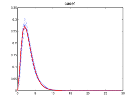
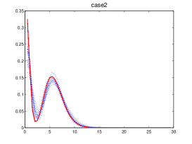
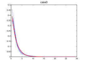
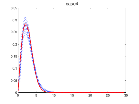
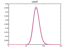
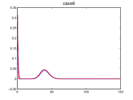
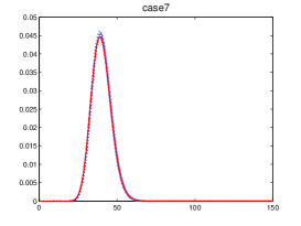
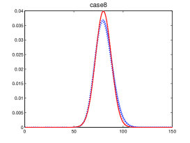
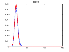
Figure 1: The true density (red) and $DD_{like}$ estimators (blue) obtained in the first 10 simulation runs with sample size $n=5000$

The first four test functions have been analyzed in Comte and Genon-Catalot (2015) and represent cases where most of the data is concentrated near zero. The 5-th test function corresponds to the situation where most of the data is concentrated away from zero. The last four test functions represent the mixtures of the two previous scenarios. All nine densities are showed in Figure 1.

Tables 1, 3 and 5 below display the average values of $\Delta_{g}$ defined in (5.1) while Tables 2, 4 and 6 report $\Delta_{\nu}$ given by (5.2) (with the standard deviations in parentheses) over 100 different realizations of data $Y_{i}\sim Poisson(\lambda_{i})$, $i=1,..,n$, where $n=10000$ for Tables 1 and 2, $n=5000$ for Tables 3 and 4 and $n=1000$ for Tables 5 and 6. The dictionary was constructed as a collection of the gamma pdfs (2.1) where parameters $(a_{k},b_{k})$ belong to the Cartesian product of vectors $a=[2,3,4,\cdots,150]$ and $b=[0.1,0.15,\cdots,0.9,0.95]$, so that $\phi_{k}(0)=0$. We chose the grid step $h=0.5$.

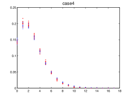
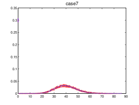
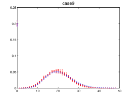
Figure 2: Sample frequencies (red) and estimated frequencies (blue) obtained in the first 10 simulation runs with sample size $n=5000$

As it is expected, performances of all estimators deteriorate when $n$ decreases, although not very significantly. For a fixed sample size, estimator $OPT$ is the most precise in terms of $\Delta_{g}$ as a direct consequence of its definition, however, estimator $DD_{like}$ is always comparable. Estimator $DD_{l2}$ has similar performance to $DD_{like}$ except for cases 2 and 6 where the underlying densities are bimodal and, hence, data can be explained by a variety of density mixtures. In conclusion, apart from $OPT$ which is not available in the case of real data, estimator $DD_{like}$ turns out to be the most accurate in terms of both $\Delta_{g}$ and $\Delta_{\nu}$. For completeness, Figures 1 and 2 exhibit some reconstructions obtained using estimator $DD_{like}$ in case of $n=5000$.

Finally, we should mention that $NDE$ is a projection estimator that uses only the first few Laguerre functions. For this reason, it fails to adequately represent a density function that corresponds to the situation where values $\lambda_{i}$, $i=1,\cdots,n$, are concentrated away from zero, as it happens in case 5 (where $NDE$ returns zero as an estimator) and case 6 (where $NDE$ succeeds in reconstructing only the first part of the density near zero). Also, note that $NDE$ errors are not displayed for cases 7, 8 and 9 since this estimator is not defined for delta contaminated densities.

6 Application to evaluation of the density of the Saturn ring

The Saturn’s rings system can be broadly grouped into two categories: dense rings (A, B, C) and tenuous rings (D, E, G) (see the first panel of Figure 3). The Cassini Division is a ring region that separates the A and B rings. The study of structure within Saturn’s rings originated with Campani, who observed in 1664 that the inner half of the disk was brighter than the outer half. Furthermore, in 1859, Maxwell proved that the rings could not be solid or liquid but were instead made up of an indefinite number of particles of various sizes, each on its own orbit about Saturn. Detailed ring structure was revealed for the first time, however, by the 1979 Pioneer and 1980-1981 Voyager encounters with Saturn. Images were taken at close range, by stellar occultation (observing the flickering of a star as it passes behind the rings), and by radio occultation (measuring the attenuation of the spacecraft’s radio signal as it passes behind the rings as seen from Earth) (see, e.g., Esposito et al, 2004). By analyzing the intensity of star light while it is passing through Saturn’s rings, astronomers can gain insight into properties telescopes cannot visually determine. Each sub-region in the rings has its own associated distinct distribution of of the density and sizes of the particles constituting the sub-region. This distribution uniquely determines the amount of light which is able to pass from a star (behind the rings) to the photometer.

Our data $Y_{i},\ i=1,\cdots,n,$ come from sets of observations of stellar occultations recorded by the Cassini UVIS high speed photometer and contains $n=7\,615\,754$ photon counts at different radial points, located at 0.01-0.1 kilometer increments, on the Saturn’s rings plane (see the second panel of Figure 3). With no outside influences, these photon counts should follow the Poisson distribution, however, obstructions imposed by the particles in the rings cause their distribution to deviate from Poisson. Indeed, if data were Poisson distributed, then its mean would be approximately equal to its variance for every sub-region. However, as the third panel of Figure 3 shows, observations $Y_{i}$ have significantly higher variances than means. The latter is due to the fact that, although for each $i=1,\cdots,n$, the photon counts $Y_{i}$ are $Poisson(\lambda_{i})$, the values of $\lambda_{i}$, $i=1,\cdots,n$, are extremely varied and, specifically, cannot be modeled as values of a continuous function. In fact, intensities $\lambda_{i}$, $i=1,\cdots,n$, are best described as random variables with an unknown underlying pdf $g(\lambda)$. In addition, if the ring region contains a significant proportion of large particle, those particles can completely block of the light leading to zero photon counts. For this reason, we allow $g(\lambda)$ to possibly contain a non-zero mass at $\lambda=0$, hence, being of the form (1.2). The shape of $g(\lambda)$ allows one to determine the density and distribution of the sizes of the particles of a respective sub-region of the Saturn rings. This information, in turn, should shed light on the question of the origin of the rings as well as how they reached their current configuration.

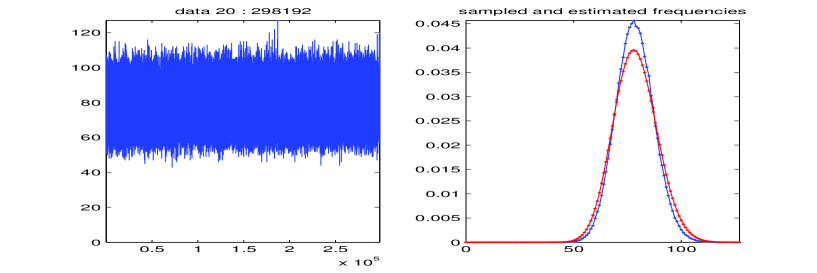
Figure 4: Left panels: segments of data. Right panels: sample frequencies (blue) and estimated frequencies with the penalty parameter obtained by $DD_{like}$ criterion (red). $\Delta_{\nu}=0.0128$ (top panel), $\Delta_{\nu}=0.0159$ (middle panel), $\Delta_{\nu}=0.0022$, $\hat{\pi}_{0}=0$ for all three cases. (bottom panel)

In order to identify sub-regions of the Saturn rings with distinct properties, we segmented the data using a method presented in [5] which is designed for partitioning of complicated signals with several non-isolated and oscillating singularities. In particular, we applied the Gabor Continuous Wavelet Transform (see, e.g. [21]) to the data and selected the highest scale where the number of wavelet modulus maxima takes minimum value. At this scale, we segmented the signal by the method proposed in [5]. We obtained a total of 1531 intervals of different sizes. Figures 4 and 5 refer to six distinct sub-regions of the rings. The left panels of both figures show raw data. The right panels exhibit the sample and the estimated frequencies, with the penalty parameter obtained by $DD_{like}$ criterion, for six different intervals that are representative of different portions of the data set.

Note that in Figure 4, for all three data segments, the estimated parameter $\hat{\pi}_{0}=0$. This is not true for the first and the second panels of Figure 5 where $\hat{\pi}_{0}=0.5059$ and $\hat{\pi}_{0}=0.2463$, respectively. The values of $\Delta_{\nu}$, defined in (5.2), obtained for the six data segments are, respectively, 0.0128, 0.0159, 0.0022, 0.0229, 0.003 and 0.0095, and are consistent with the values obtained in simulations. Both, the right panels in Figures 4 and 5 and the values of $\Delta_{\nu}$, confirm the ability of the estimator developed in the paper to accurately explain the Saturn’s rings data.

7 Proofs

Proofs of Theorems 1 and 2 are based on the following statement which is the trivial modification of Lemma 3 of Pensky (2015).

Lemma 1

(Pensky (2015)). Let $f$ be the true function and $f_{\mbox{$\theta$}}$ be its projection onto the linear span of the dictionary ${\mathcal{L}}_{{\mathcal{P}}}$. Let $\Upsilon$ be a diagonal matrix with components $\sigma_{j}$, $j=1,\cdots,p$. Consider solution of the weighted Lasso problem

$$\widehat{\mbox{$\theta$}}=\arg\min_{\mathbf{t}}\left\{\mathbf{t}^{T}\mathbf{W}\mathbf{W}^{T}\mathbf{t}-2\mathbf{t}^{T}\widehat{\mbox{$\beta$}}+\alpha\|\mbox{$\Upsilon$}\mathbf{t}\|_{1}\right\}.$$ (7.1)

with $\mbox{$\Phi$}=\mathbf{W}^{T}\mathbf{W}$, $\mbox{$\beta$}=\mbox{$\Phi$}\mbox{$\theta$}$ and

$$\widehat{\mbox{$\beta$}}=\mbox{$\beta$}+\sqrt{\varepsilon}\mbox{$\Upsilon$}\mbox{$\eta$}+\mathbf{h},\quad\mbox{$\eta$},\mathbf{h}\in{\mathbb{R}}^{p},$$ (7.2)

where $\mathbf{h}$ is a nonrandom vector, ${\mathbb{E}}\mbox{$\eta$}=0$ and components $\eta_{j}$ of vector $\eta$ are random variables such that, for some $K>0$ and any $\tau>0$, there is a set

$$\Omega=\left\{\omega:\max_{1\leq j\leq p}|\eta_{j}|\leq K\sqrt{(\tau+1)\log p}\right\}\quad\mbox{with}\quad{\mathbb{P}}(\Omega)\geq 1-2p^{-\tau}.$$ (7.3)

Denote

$$C_{h}=\max_{1\leq j\leq p}\left[\frac{|h_{j}|}{\sigma_{j}\,\sqrt{\varepsilon\,\log p}}\right],\quad\quad C_{\alpha}=K\sqrt{\tau+1}+C_{h}.$$ (7.4)

If $\alpha_{0}=C_{\alpha}\sqrt{\varepsilon\log p}$, then for any $\tau>0$ and any $\alpha\geq\alpha_{0}$, then, with probability at least $1-2p^{-\tau}$, one has

$$\|f_{\widehat{\mbox{$\theta$}}}-f\|_{2}^{2}\leq\inf_{\mathbf{t}}\left[\|f_{\mathbf{t}}-f\|_{2}^{2}+4\alpha\|\mbox{$\Upsilon$}\mathbf{t}\|_{1}\right].$$ (7.5)

Moreover, if matrices $\Phi$ and $\Upsilon$ are such that for some $\mu>1$ and any $J\subset{\mathcal{P}}$

$$\kappa^{2}(\mu,J)=\min\left\{\mathbf{d}\in{\mathcal{D}}(\mu,J),\,\|\mathbf{d}\|_{2}\neq 0:\quad\frac{\mathbf{d}^{T}\mbox{$\Phi$}\mathbf{d}\cdot\mbox{Tr}(\mbox{$\Upsilon$}_{J}^{2})}{\|(\mbox{$\Upsilon$}\mathbf{d})_{J}\|_{1}^{2}}\right\}>0,$$ (7.6)

and $\alpha=\varpi\alpha_{0}$ where $\varpi\geq(\mu+1)/(\mu-1)$, then for any $\tau>0$ with probability at least $1-2p^{-\tau}$, one has

$$\|f_{\widehat{\mbox{$\theta$}}}-f\|_{2}^{2}\leq\inf_{\mathbf{t},J\subseteq{\mathcal{P}}}\left[\|f_{\mathbf{t}}-f\|_{2}^{2}+4\alpha\|(\mbox{$\Upsilon$}\mathbf{t})_{{J^{c}}}\|_{1}+\frac{(1+\varpi)^{2}C_{\alpha}^{2}}{\kappa^{2}(\mu,J)}\varepsilon\log p\ \sum_{j\in J}\sigma_{j}^{2}\right].$$ (7.7)

Proof of Theorem 1.   Let vectors $\mathbf{b}$ and $\xi$, respectively, have components $b_{k}=\langle\phi_{k},f\rangle$ and $\xi_{k}$ defined in (2.16). It is easy to see that

$$\xi_{k}-b_{k}=\frac{1}{n}\sum_{i=1}^{n}[\psi_{k}(Y_{i})-{\mathbb{E}}\psi_{k}(Y_{i})]+H_{k}\quad\mbox{with}\quad H_{k}={\mathbb{E}}\widetilde{\psi}_{k,\widehat{\zeta_{k}}}-b_{k}$$ (7.8)

Applying Bernstein inequality, for any $x>0$, obtain

$${\mathbb{P}}\left(\left|n^{-1}\,\sum_{i=1}^{n}[\psi_{k}(Y_{i})-{\mathbb{E}}\psi_{k}(Y_{i})]\right|\geq\frac{x\sigma_{k}}{\sqrt{n}}\right)\leq 2\exp\left(-x^{2}\,\left[2+\frac{4x\sigma_{k}\|\psi_{k}\|_{\infty}}{3\sqrt{n}}\right]^{-1}\right).$$

Using the fact that $A/(B+C)\geq\min(A/(2B),A/(2C))$ for any $A,B,C>0$, under condition $n\geq N_{0}$, derive

$${\mathbb{P}}\left(\left|n^{-1}\,\sum_{i=1}^{n}[\psi_{k}(Y_{i})-{\mathbb{E}}\psi_{k}(Y_{i})]\right|\geq xn^{-1/2}\,\sigma_{k}\right)\leq 2\exp-(x^{2}/4).$$ (7.9)

Choosing $x=2\sqrt{(\tau+1)\log p}$ and recalling that, according to (2.10), $|H_{k}|=n^{-1/2}\sigma_{k}$, gather that ${\mathbb{P}}(|\xi_{k}-b_{k}|>n^{-1/2}\,\sigma_{k}[2\sqrt{(\tau+1)\log p}+1])\leq p^{-(\tau+1)}$, so that

$$\Omega_{1}=\left\{\omega:\ \max_{1\leq k\leq p}\,\left[\frac{|\xi_{k}-b_{k}|}{\sigma_{k}}\right]\leq\frac{2\sqrt{(\tau+1)\log p}+1}{\sqrt{n}}\right\}\quad\mbox{with}\quad{\mathbb{P}}(\Omega_{1})>1-2p^{-\tau}.$$ (7.10)

Then, validity of Theorem 1 follows directly from Lemma 1 with $\eta_{k}=\xi_{k}/\sigma_{k}$ and $K=2$.

Proof of Theorem 2. Validity of inequality (4.11) follows from (7.10) and Lemma 1 with $K=2$.

In order to establish upper bounds for $(\hat{\pi}_{0}-\pi_{0})^{2}$, note that ${\mathbb{P}}(Y=0)=\pi_{0}+\mbox{$\theta$}^{T}\mathbf{u}$, so that

$$\hat{\pi}_{0}-\pi_{0}=\left\{\begin{array}[]{ll}\nu_{0}-{\mathbb{P}}(Y=0)-\mathbf{d}^{T}\mathbf{u},&\mbox{if}\ \ \nu_{0}-\widehat{\mbox{$\theta$}}^{T}\mathbf{u}\geq 0,\\ -\pi_{0},&\mbox{if}\ \ \nu_{0}-\widehat{\mbox{$\theta$}}^{T}\mathbf{u}<0,\end{array}\right.$$ (7.11)

where $\mathbf{d}=\widehat{\mbox{$\theta$}}-\mbox{$\theta$}_{0}$. Then, by standard arguments (see, e.g. Dalalyan et al. (2014)), one has

$$\mathbf{d}^{T}\mbox{$\Phi$}\mathbf{d}\leq\mathbf{d}^{T}(\mbox{$\xi$}-\mathbf{b})+\alpha(\|\mbox{$\Upsilon$}\mbox{$\theta$}_{0}\|_{1}-\|\mbox{$\Upsilon$}\hat{\mbox{$\theta$}}\|_{1})$$

For $\omega\in\Omega_{1}$ where $\Omega_{1}$ is defined in (7.10), one has

$$\mathbf{d}^{T}\mbox{$\Phi$}\mathbf{d}+(\alpha-\alpha_{0})\|(\mbox{$\Upsilon$}\mathbf{d})_{J_{0}^{c}}\|_{1}\leq(\alpha+\alpha_{0})\|(\mbox{$\Upsilon$}\mathbf{d})_{J_{0}}\|_{1}.$$ (7.12)

Therefore, $\mathbf{d}\in{\mathcal{D}}(\mu,J_{0})$ where ${\mathcal{D}}(\mu,J)$ is defined in (4.3), and due to $J_{0}\in{\mathcal{G}}(C_{\sigma})$, the following inequality holds:

$$\|\mathbf{d}_{J_{0}^{c}}\|_{1}\leq\mu C_{\sigma}\|\mathbf{d}_{J_{0}}\|_{1}.$$ (7.13)

Hence, by (4.9), $\mathbf{d}^{T}\mbox{$\Phi$}\mathbf{d}\geq\vartheta(s,m,\mu,C_{\sigma})$. On the other hand, inequality (7.12) yields $\mathbf{d}^{T}\mbox{$\Phi$}\mathbf{d}\leq(\alpha+\alpha_{0})\|\mathbf{d}_{J_{0}}\|_{2}\sqrt{\mbox{Tr}(\mbox{$\Upsilon$}_{J_{0}}^{2})}$, so that

$$\|\mathbf{d}_{J_{0}}\|_{2}\leq\frac{(\alpha+\alpha_{0})}{\vartheta(s,m,\mu,C_{\sigma})}\ \sqrt{\mbox{Tr}(\mbox{$\Upsilon$}_{J_{0}}^{2})}.$$ (7.14)

Using (7.13) and (7.14), obtain that, for any $\omega\in\Omega_{1}$,

$$|\mathbf{d}^{T}\mathbf{u}| \leq \|\mathbf{d}_{J_{0}}\|_{1}\|\mathbf{u}_{J_{0}}\|_{\infty}+\|\mathbf{d}_{J_{0}^{c}}\|_{1}\|\mathbf{u}_{J_{0}^{c}}\|_{\infty}\leq\|\mathbf{d}_{J_{0}}\|_{1}\|\mathbf{u}\|_{\infty}(1+\mu C_{\sigma})$$

$$\leq \sqrt{s}\|\mathbf{d}_{J_{0}}\|_{2}\|\mathbf{u}\|_{\infty}(1+\mu C_{\sigma})\leq\sqrt{s}\,\alpha_{0}\,(1+\varpi)\|\mathbf{u}\|_{\infty}(1+\mu C_{\sigma})\ \sqrt{\mbox{Tr}(\mbox{$\Upsilon$}_{J_{0}}^{2})}/\vartheta(s,m,\mu,C_{\sigma}).$$

In addition, there exists a set $\Omega_{2}$ such that, for $\omega\in\Omega_{2}$, one has $|\nu_{0}-{\mathbb{P}}(Y=0)|\leq\sqrt{(\tau\log p)/n}$ and ${\mathbb{P}}(\Omega_{2})\geq 1-2p^{-\tau}$. Let $\Omega=\Omega_{1}\cap\Omega_{2}$. Then, ${\mathbb{P}}(\Omega)\geq 1-4p^{-\tau}$ and, for $\omega\in\Omega$,

$$|\nu_{0}-{\mathbb{P}}(Y=0)-\mathbf{d}^{T}\mathbf{u}|\leq\frac{\sqrt{s}\,\alpha_{0}\,\sqrt{\mbox{Tr}(\mbox{$\Upsilon$}^{2}_{J_{0}})}\,(1+\varpi)\,\|\mathbf{u}\|_{\infty}(1+\mu C_{\sigma})}{\vartheta(s,m,\mu,C_{\sigma})}\,+\frac{\sqrt{\tau\log p}}{\sqrt{n}}.$$ (7.15)

Inequality (7.15) provides an upper bound for the error if $\nu_{0}-\widehat{\mbox{$\theta$}}^{T}\mathbf{u}\geq 0$. If $\nu_{0}-\widehat{\mbox{$\theta$}}^{T}\mathbf{u}<0$, note that

$$0\leq\pi_{0}=({\mathbb{P}}(Y=0)-\nu_{0}-\mathbf{d}^{T}\mathbf{u})+(\nu_{0}-\widehat{\mbox{$\theta$}}^{T}\mathbf{u})\leq{\mathbb{P}}(Y=0)-\nu_{0}-\mathbf{d}^{T}\mathbf{u},$$

and again apply (7.15). Finally, plugging in the value of $\alpha_{0}$ and using inequality for $H_{0}$, derive that, for $\omega\in\Omega$, inequality (4.12) holds.

Table 1: Average values of $\Delta_{g}$ (with their standard deviations in parentheses) over 100 simulation runs with $n=10000$

test case	$OPT$	$DD_{l2}$	$DD_{like}$	$NDE$
case1	0.0007 (0.0010)	0.0023 (0.0028)	0.0022 (0.0030)	0.1183 (0.8307)
case2	0.0471 (0.0197)	0.2214 (0.0503)	0.0507 (0.0305)	0.0613 (0.0716)
case3	0.0142 (0.0398)	0.0191 (0.0127)	0.0138 (0.0087)	0.0190 (0.0399)
case4	0.0043 (0.0021)	0.0054 (0.0032)	0.0061 (0.0052)	0.0298 (0.0657)
case5	0.0042 (0.0033)	0.0023 (0.0029)	0.0014 (0.0021)	1.0000 (0.0000)
case6	0.0793 (0.0247)	0.4318 (0.0554)	0.0839 (0.0241)	0.3383 (0.0085)
case7	0.0067 (0.0012)	0.0009 (0.0008)	0.0008 (0.0008)	-
case8	0.0060 (0.0010)	0.0068 (0.0009)	0.0069 (0.0010)	-
case9	0.0085 (0.0013)	0.0099 (0.0014)	0.0111 (0.0026)	-

Table 2: Average values of $\Delta_{\nu}$ (with their standard deviations in parentheses) over 100 simulation runs with $n=10000$

test case	$OPT$	$DD_{l2}$	$DD_{like}$	$NDE$
case1	0.0011 (0.0009)	0.0006 (0.0005)	0.0007 (0.0005)	0.0675 (0.5470)
case2	0.0013 (0.0007)	0.0088 (0.0024)	0.0014 (0.0010)	0.0228 (0.0431)
case3	0.0002 (0.0001)	0.0006 (0.0005)	0.0003 (0.0003)	0.1130 (0.0653)
case4	0.0014 (0.0009)	0.0011 (0.0006)	0.0012 (0.0009)	0.0205 (0.0530)
case5	0.0045 (0.0010)	0.0043 (0.0010)	0.0044 (0.0009)	1.0000 (0.0000)
case6	0.0465 (0.1402)	0.0288 (0.0045)	0.0041 (0.0020)	0.4376 (0.0618)
case7	0.0013 (0.0002)	0.0006 (0.0002)	0.0006 (0.0002)	-
case8	0.0039 (0.0009)	0.0018 (0.0004)	0.0018 (0.0004)	-
case9	0.0035 (0.0006)	0.0019 (0.0007)	0.0020 (0.0006)	-

Table 3: Average values of $\Delta_{g}$ (with their standard deviations in parentheses) over 100 simulation runs with $n=5000$

test case	$OPT$	$DD_{l2}$	$DD_{like}$	$NDE$
case1	0.0006 (0.0008)	0.0038 (0.0049)	0.0030 (0.0046)	0.2424 (1.5002)
case2	0.0590 (0.0343)	0.2106 (0.0549)	0.0640 (0.0428)	0.2048 (0.2196)
case3	0.0148 (0.0097)	0.0251 (0.0310)	0.0178 (0.0119)	0.0309 (0.0650)
case4	0.0055 (0.0019)	0.0074 (0.0051)	0.0086 (0.0060)	0.0493 (0.1123)
case5	0.0069 (0.0052)	0.0044 (0.0048)	0.0024 (0.0036)	1.0000 (0.0000)
case6	0.0830 (0.0277)	0.4068 (0.0856)	0.0879 (0.0266)	0.3456 (0.0110)
case7	0.0077 (0.0035)	0.0023 (0.0030)	0.0023 (0.0030)	-
case8	0.0065 (0.0021)	0.0074 (0.0020)	0.0075 (0.0021)	-
case9	0.0096 (0.0023)	0.0114 (0.0023)	0.0128 (0.0029)	-

Table 4: Average values of $\Delta_{\nu}$ (with their standard deviations in parentheses) over 100 simulation runs with $n=5000$

test case	$OPT$	$DD_{L2}$	$DD_{like}$	$NDE$
case1	0.0017 (0.0016)	0.0010 (0.0007)	0.0012 (0.0007)	0.1393 (1.0084)
case2	0.0020 (0.0013)	0.0090 (0.0029)	0.0022 (0.0014)	0.1184 (0.1475)
case3	0.0004 (0.0002)	0.0009 (0.0013)	0.0006 (0.0004)	0.1131 (0.0948)
case4	0.0022 (0.0014)	0.0016 (0.0008)	0.0018 (0.0013)	0.0346 (0.0859)
case5	0.0087 (0.0019)	0.0084 (0.0018)	0.0085 (0.0018)	1.0000 (0.0000)
case6	0.0377 (0.1361)	0.0285 (0.0068)	0.0057 (0.0030)	0.4608 (0.0849)
case7	0.0020 (0.0003)	0.0013 (0.0003)	0.0013 (0.0003)	-
case8	0.0052 (0.0011)	0.0032 (0.0008)	0.0032 (0.0008)	-
case9	0.0044 (0.0010)	0.0031 (0.0010)	0.0031 (0.0009)	-

Table 5: Average values of $\Delta_{g}$ (with their standard deviations in parentheses) over 100 simulation runs with $n=1000$

test case	$OPT$	$DD_{l2}$	$DD_{like}$	$NDE$
case1	0.0040 (0.0097)	0.0221 (0.0258)	0.0176 (0.0207)	0.3004 (0.9331)
case2	0.0992 (0.0760)	0.1973 (0.0718)	0.1335 (0.0983)	0.5370 (0.0960)
case3	0.0533 (0.0889)	0.0753 (0.0838)	0.0662 (0.0894)	0.1127 (0.3912)
case4	0.0069 (0.0014)	0.0178 (0.0183)	0.0179 (0.0135)	0.1393 (0.3381)
case5	0.0170 (0.0108)	0.0217 (0.0253)	0.0152 (0.0223)	1.0000 (0.0000)
case6	0.1223 (0.0710)	0.3151 (0.1409)	0.1270 (0.0759)	0.4479 (0.2572)
case7	0.0133 (0.0115)	0.0102 (0.0118)	0.0098 (0.0118)	-
case8	0.0142 (0.0137)	0.0156 (0.0139)	0.0156 (0.0154)	-
case9	0.0121 (0.0073)	0.0163 (0.0110)	0.0160 (0.0101)	-

Table 6: Average values of $\Delta_{\nu}$ (with their standard deviations in parentheses) over 100 simulation runs with $n=1000$

test case	$OPT$	$DD_{l2}$	$DD_{like}$	$NDE$
case1	0.0063 (0.0042)	0.0043 (0.0026)	0.0047 (0.0027)	0.1458 (0.5377)
case2	0.0076 (0.0051)	0.0117 (0.0047)	0.0084 (0.0048)	0.3498 (0.0937)
case3	0.0021 (0.0022)	0.0031 (0.0033)	0.0027 (0.0037)	0.2149 (0.3773)
case4	0.0075 (0.0068)	0.0046 (0.0029)	0.0048 (0.0032)	0.0967 (0.3578)
case5	0.0427 (0.0091)	0.0411 (0.0090)	0.0416 (0.0090)	1.0000 (0.0000)
case6	0.0157 (0.0044)	0.0304 (0.0127)	0.0166 (0.0067)	0.5344 (0.1001)
case7	0.0072 (0.0018)	0.0067 (0.0018)	0.0067 (0.0018)	-
case8	0.0154 (0.0038)	0.0143 (0.0038)	0.0142 (0.0037)	-
case9	0.0120 (0.0034)	0.0111 (0.0032)	0.0111 (0.0032)	-

Figure 3: The first panel: Names of Saturn s rings, courtesy science.nasa.gov. The second panel: the means of the binned total data set (100 observations per bin). The third panel: the means (red) and the variances (blue) of the binned data

Figure 5: Left panels: segments of data. Right panels: sample frequencies (blue) and estimated frequencies with the penalty parameter obtained by $DD_{like}$ criterion (red). $\Delta_{\nu}=0.0229$ and $\hat{\pi}_{0}=0.5059$ (top panel), $\Delta_{\nu}=0.003$ and $\hat{\pi}_{0}=0.2463$ (middle panel), $\Delta_{\nu}=0.0095$ and $\hat{\pi}_{0}=0$ (bottom panel)

References

- [1] Antoniadis, A., Sapatinas, T. (2004) Wavelet shringkage for natural exponential families with quadratic variance functions. Biometrica, 88, 805-820.
- [2] Besbeas, P., De Feis, I., Sapatinas, T. (2004) A Comparative Simulation Study of Wavelet Shrinkage Estimators for Poisson Counts. International Statistical Review, 72, 209-237.
- [3] Bickel, P.J., Ritov, Y., Tsybakov, A. (2009) Simultaneous analysis of Lasso and Dantzig selector. Ann. Statist., 37, 1705-1732.
- [4] Brown, L. D., Cai, T. T., Zhou, H. (2010). Nonparametric regression in exponential families. Ann. Statist., 38, 2005-2046.
- [5] Bruni, V., De Canditiis, D., Vitulano, D. (2012) Time-scale energy based analysis of contours of real-world shapes. Mathematics and Computer in Simulation, 82, 2891-2907.
- [6] Bühlmann, P., van de Geer, S. (2011) Statistics for High-Dimensional Data: Methods, Theory and Applications, Springer.
- [7] Chow, Y.-S., Geman, S., Wu, L.-D. (1983) Consistent cross-validated density estimaton. Ann. Statist., 11, 25-38.
- [8] Colwell, J.E., Nicholson, P.D., Tiscareno, M.S., Murray, C.D., French, R.G., Marouf, E.A. (2009) The Structure of Saturn s Rings. In Saturn from Cassini-Huygens, Dougherty, M., Esposito, L., Krimigis, S. Eds., Springer.
- [9] Comte, F., Genon-Catalot, V. (2015) Adaptive Laguerre density estimation for mixed Poisson models. Electr. Journ. Statist., 9, 1113-1149.
- [10] Dalalyan, A.S., Hebiri, M., Lederer, J. (2014) On the prediction performance of the Lasso. arxiv: 1402.1700
- [11] Esposito, L. W., Barth, C. A. , Colwell, J. E., Lawrence, G. M., McClintock, W. E., Stewart, A. I. F., Keller, H. U., Korth, A., Lauche, H., Festou, M. C., Lane, A. L., Hansen, C. J., Maki, J. N., West, R. A., Jahn, H., Reulke, R., Warlich, K., Shemansky, D. E., Yung, Y. L. (2004) The Cassini Ultraviolet Imaging Spectrograph investigation. Space Sci. Rev., 115, 294-361.
- [12] Fryzlewicz, P., Nason G.P. (2004) A Haar-Fisz Algorithm for Poisson Intensity Estimation. Journ. Computat. Graph. Statis., 13, 621-638.
- [13] Harmany, Z., Marcia, R., Willett, R. (2012) This is SPIRAL-TAP: Sparse Poisson Intensity Reconstruction ALgorithms Theory and Practice. IEEE Trans. Image Processing, 21, 1084-1096.
- [14] He, S., Yang, G.L., Fang, K.T., Widmann, J.F. (2005) Estimation of Poisson Intensity in the Presence of Dead Time Journ. Amer. Statist. Assoc. 100, 669-679.
- [15] Herngartner, N.W. (1997) Adaptive demixing in Poisson mixture models. Ann. Stat., 25, 917-928.
- [16] Hirakawa, K., Wolfe, P.J. (2012) Skellam Shrinkage: Wavelet-Based Intensity Estimation for Inhomogeneous Poisson Data IEEE Trans. Inf. Theory, 58, 1080-1093.
- [17] Jansen, M. (2006) Multiscale Poisson data smoothing. J. R. Statist. Soc., Ser. B, 68, 27-48.
- [18] Kolaczyk, E.D. (1999) Bayesian Multiscale Models for Poisson Processes. Journ. Amer. Statist. Assoc., 94, 920-933.
- [19] Lambert, D., Tierney, L. (1984) Asymptotic properties of maximum likelihood estimates in the mixed Poisson model. Ann. Statist., 12, 1388-1399.
- [20] Lord, D., Washington, S.P., Ivan, J.N. (2005) Poisson, Poisson-gamma and zero-inflated regression models of motor vehicle crashes: balancing statistical fit and theory. Accid. Anal. Prevent., 37, 35-46.
- [21] Mallat, S. (2009) A Wavelet Tour of Signal Processing: The Sparse Way, 3rd ed. Elsevier.
- [22] Pensky, M. (2015) Solution of linear ill-posed problems using overcomplete dictionaries. ArXiv 1408.3386v2.
- [23] Timmermann, K.E., Nowak, R.D. (1999) Multiscale Modeling and Estimation of Poisson Processes with Application to Photon-Limited Imaging. IEEE Trans. Inf. Theory, 45, 846-862.
- [24] Walter, G. (1985) Orthogonal polynomials estimators of the prior distribution of a compound Poisson distribution. Sankhya, Ser. A, 47, 222-230.
- [25] Walter, G. and Hamedani, G. (1991) Bayes empirical Bayes estimation for natural exponential families with quadratic variance function. Ann. Statist., 19, 1191-1224.
- [26] Zhang, C.-H. (1995) On estimating mixing densities in discrete exponential family models. Ann. Statist., 23, 929-947.
- [27] Zou, H., Hastie, T. (2005) Regularization and variable selection via the elastic net. JRSS, Ser.B, 67, Part 2, 301-320.