Universal set of Dynamically Protected Gates for Bipartite Qubit Networks II:
Soft Pulse Implementation of the [[5,1,3]] Quantum Error Correcting Code.

Abstract

We model repetitive quantum error correction (QEC) with the single-error-correcting five-qubit code on a network of individually-controlled qubits with always-on Ising couplings, using our previously designed universal set of quantum gates based on sequences of shaped decoupling pulses. In addition to serving as accurate quantum gates, the sequences also provide dynamical decoupling (DD) of low-frequency phase noise. The simulation involves integrating unitary dynamics of six qubits over the duration of tens of thousands of control pulses, using classical stochastic phase noise as a source of decoherence. The combined DD/QEC protocol dramatically improves the coherence, with the QEC alone responsible for more than an order of magnitude infidelity reduction.

I INTRODUCTION

Quantum error correctionShor (1995); Gottesman (1997); Knill and Laflamme (1997); Terhal (2015) (QEC) makes it possible to perform large scale quantum computations with a finite error rate per qubitShor (1996); Steane (1997); Gottesman (1998); Dennis et al. (2002); Knill (2003); Knill et al. (1998); Steane (2003). Much like their classical counterparts, quantum error correcting codes (QECCs) rely on adding redundant qubits to control errors. However, unlike, e.g., in the classical information transmission problem, qubits remain subject to errors all the time, in particular, during the syndrome extraction. Thus, to achieve scalability, special fault-tolerant (FT) protocols must be used both for QEC and for any operation with the encoded qubits. This increases the overhead and is one of the reasons why the error probability thresholds to scalable quantum computation are so small—e.g., around $1\%$ per local gate in the case of the toric and related surface codesKitaev (2003); Dennis et al. (2002); Raussendorf and Harrington (2007). The number of qubits needed, measurement complexity, and stringent requirements for gate speed and fidelity are also among the reasons why an experimental demonstration of the repetitive quantum error correction with a universal quantum code so far remains an elusive goal.Cory et al. (1998); Chiaverini et al. (2004); Pittman et al. (2005); Schindler et al. (2011); Moussa et al. (2011); Reed et al. (2012); Barends et al. (2013); Zhong et al. (2014); Chow et al. (2014); Barends et al. (2014); Córcoles et al. (2015); Kelly et al. (2015)

A possible way to loosen these requirements is to combine active QEC with one of the passive error reduction techniques depending on the correlations in the dominant decoherence channelLidar et al. (1998); Viola et al. (1999a, b); Lidar et al. (1999); Bacon et al. (2000); Kempe et al. (2001); Viola (2002); Facchi et al. (2005); Lidar (2014). In particular, dynamical decoupling (DD) is most effectiveShiokawa and Lidar (2004); Faoro and Viola (2004); Sengupta and Pryadko (2005); Pryadko and Sengupta (2006); Kuopanportti et al. (2008); Cywiński et al. (2008); West et al. (2010) in suppressing the effects of low-frequency (e.g., $1/f$) noise which is often the leading mechanism for the loss of phase coherence. Moreover, DD can be used to achieve scalability in gate design, since pulses and sequences intended for a large system can be constructed to a given order in the Magnus seriesSlichter (1992) on small qubit clustersSengupta and Pryadko (2005); Pryadko and Sengupta (2006). DD is also excellent in producing accurate control for systems where not all interactions are known as one can decouple interactions with the given symmetryStollsteimer and Mahler (2001); Tomita et al. (2010), and it can be implemented to remain stable when environment has sharp spectral featuresPryadko and Quiroz (2007) or high-frequency modesPryadko and Quiroz (2009), or even with substantial pulse errorsPryadko and Sengupta (2008); Kabytayev et al. (2014). In short, at least in principle, using DD at the lowest level of coherence protection could substantially reduce the required repetition rate of the QEC cycle. In many instances, this could make a crucial difference, enabling the use of QEC.

Recently we made a substantial progress toward developing a combined DD/QEC coherence protection protocol by constructing a universal set of quantum gates based on soft-pulse DD sequences.De and Pryadko (2013a, 2014) The gates are designed to work on a network of qubits with always-on Ising couplings forming a sparse bipartite graph. In addition to providing accurate control, these gates also work as decoupling sequences, suppressing the effect of low-frequency phase noise to second order in the Magnus series. With these gates, we demonstratedDe and Pryadko (2013a) the effectiveness of repetitive QEC using single-error-detecting QECC $[[4,2,2]]$ encoding two qubits in four by simulating full unitary dynamics of five driven qubits in an Ising chain, using low-frequency classical noise as the source of decoherence.

We have also studiedDe and Pryadko (2014) the errors associated with the gates similar to those constructed in Ref. De and Pryadko, 2013a. In a system with always-on pairwise qubit couplings, for any gate constructed perturbatively to a given order $K$, only the errors forming clusters that involve up to $K+1$ qubits are suppressed. Large-weight clusters of correlated errors can be suppressed exponentially when gates are executed fast enough. However, such a choice can only be made with a sufficiently sparse coupling network. Increasing the maximum degree $z$ of the connectivity graph with pulse duration and other gates’ parameters fixed may lead to proliferation of large uncorrectable error clusters.

In our previous workDe and Pryadko (2013a), we simulated a linear Ising chain with $z=2$, an arrangement most favorable for controlling multi-qubit correlated errors. On the other hand, the optimal arrangement for surface codes is planar. The corresponding analytical bound on maximum gate duration needed for FT is smallDe and Pryadko (2014). Thus, it remains an open question whether perturbation-theory-based gates like those constructed in Ref. De and Pryadko, 2013a can be practical for use in repetitive QEC.

In this work we simulate numerically repetitive quantum error correction using our universal gate setDe and Pryadko (2013a, 2014) in a network with $z\geq 4$ as would be needed for the surface code. Specifically, we use a six-qubit star graph (see Fig. 1) of Ising couplings between the qubits with $z=5$, and simulate QEC with the $[[5,1,3]]$ code both in the traditional and in the error-detection (Zeno) modes. This code can actually be seen as a variant of a surface code with rotated periodicity vectors.Kovalev et al. (2011); Kovalev and Pryadko (2012) We simulate full unitary dynamics over several error correcting cycles (up to seventy thousand shaped pulses) with instantaneous ancilla-based projective measurements, and classical Gaussian correlated phase noise used as a source of decoherence. We consider the cases of low-frequency noise with Gaussian correlations, as well as a bimodal noise generated as a combination of a low-frequency and a high-frequency components. The constructed protocols show substantial improvement of coherence compared to the case of unprotected qubits, including over an order of magnitude average infidelity reduction attributable to error correction alone.

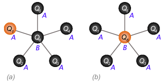
Figure 1: (Color online) Arrangement of qubits on a bipartite star graph for implementing the [[5,1,3]] code. This particular arrangement of the qubits was chosen to minimize the total number of gate operation during the stabilizer generator measurement cycle. (a) The qubit to be encoded, $Q_{6}$, is initially placed at the center. At the end of encoding, it is swapped with an ancilla qubit, initially $Q_{1}$. (b) During the stabilizer measurement cycle, the single ancilla qubit $Q_{6}$ at the center is used to sequentially measure all four stabilizer generators supported by the five qubits around it.

The structure of the paper is as follows. In Sec. II, we give a brief overview of dynamical decoupling, of the universal gate set used, and our implementation of the $[[5,1,3]]$ code on a star graph. In Sec. III, we present the results of numerical simulations. We give Conclusions in Sec. IV.

II Gate and code implementation

II.1 Dynamical control on an Ising network

The goal of dynamical control is to drive the desired unitary evolution of a quantum system over a given time interval. While the details of the dynamics during the interval may differ greatly, the net result of such an evolution can be, to some extent, insensitive to the details of system’s interactions. For example, in the simplest case of single-qubit dynamical decoupling, the qubit interactions are averaged out during the period of the controlled evolution.

We consider the following general Hamiltonian

$$H=H_{\mathrm{C}}+H_{0},\quad H_{0}=H_{\rm S}+H_{\rm B}+H_{\rm SB},$$ (1)

where $H_{\mathrm{C}}\equiv H_{\rm C}(t)$ is the time-dependent control Hamiltonian, and the remaining Hamiltonian $H_{0}$ is separated into the parts $H_{\mathrm{S}}$ and $H_{\rm B}$ acting on the qubit “system” and on the bath respectively, and the system-bath coupling Hamiltonian $H_{\rm SB}$.

In this work, following Refs. De and Pryadko, 2013a, 2014, we consider a sparse bipartite network of qubits with the Ising couplings between nearest neighbors,

$$H_{\rm S}\equiv{1\over 2}\sum_{\langle i,j\rangle}J_{ij}\sigma^{z}_{i}\sigma^{z}_{j},$$ (2)

and decoherence due to slow dephasing of individual qubits, generally described by the following bath and bath-coupling Hamiltonians:

$$H_{\rm B}=\sum_{i}B_{i},\quad H_{\rm SB}={1\over 2}\sum_{i}A_{i}\sigma_{i}^{z}.$$ (3)

Each qubit is assumed to have its own individual bath, i.e., the bath operators $B_{j}$ commute with each other, and the coupling operators $A_{i}$ commute with each other and all $B_{j}$, $j\neq i$.

The decoupling technique assumes that the control Hamiltonian $H_{\rm C}$ dominates the dynamics. We implicitly assume that any large energies have already been eliminated from the system $H_{\rm S}$ and system-bath coupling $H_{\rm SB}$ Hamiltonians by a rotating wave approximation (RWA). Then, the Hamiltonian (2) can be viewed as an effective Hamiltonian for any set of interactions as long as the transition frequencies of the neighboring qubits differ sufficiently. Similarly, the bath model (3) is an effective description of qubits operating well above the bath frequency cut-off to eliminate direct spin flip transitions, with dephasing caused, say, by phonon scattering.

We also assume the ability to control the qubits individually, with the control Hamiltonian

$$H_{\rm C}\equiv\sum_{j}H_{\rm C}^{(j)},\quad H_{\rm C}^{(j)}={1\over 2}\sum_{\mu=x,y,z}V_{j\mu}(t)\,\sigma_{j}^{\mu},$$ (4)

where the time dependent control signals $V_{j\mu}(t)$ are arbitrary, except for some implicit limits on their amplitude and spectrum. Our gatesDe and Pryadko (2013a, 2014) are designed as sequences of one-dimensional pulses, with the control fields on a given qubit applied along $x$, $y$, or $z$ axis exclusively, so that only one of $V_{x}(t)$, $V_{y}(t)$, or $V_{z}(t)$ can be non-zero at any given time. We also imposed a restriction that no pulses be applied simultaneously on any pair of neighboring qubits.

As a result of these assumptions, the multi-qubit unitary evolution operator with the complete Hamiltonian (1) over the duration of a single-pulse interval can be written as a product of mutually commuting terms, each of them involving the controlled qubit and various products of $\sigma^{z}$ Pauli operators for its uncontrolled neighbors.De and Pryadko (2014) Each of these operators can be computed order-by-order in the time-dependent perturbation theory; in Ref. De and Pryadko, 2014 we carried such an expansion up to third order. In each order of the series, the dependence on the pulse shape is encoded in terms of just a few coefficientsPryadko and Quiroz (2007); Pryadko and Sengupta (2008); Pryadko and Quiroz (2009); De and Pryadko (2014). For example, the first-order correction is expressed in terms of just two such coefficients, the time averages of $\cos\phi(t)$ and $\sin\phi(t)$ over the duration of the pulse, where $\phi(t)=\int_{0}^{t}dt^{\prime}V(t^{\prime})$ is the time-dependent rotation angle corresponding to the given pulse shape $V(t)$, $0\leq t\leq\tau_{p}$, and $\tau_{p}$ is the pulse duration. With generic pulse shapes, such as a Gaussian, this produces errors that scale linearly with $\tau_{p}$. Specially designed self-refocusing pulses can be constructed to suppress this effect, e.g., to linear or quadratic orders in powers of $\tau_{p}$, depending on the shapeSengupta and Pryadko (2005); Pryadko and Sengupta (2008). For example, to the linear order, this is done by choosing a functional form $V(t)$ which guarantees $\langle\cos\phi(t)\rangle=\langle\sin\phi(t)\rangle=0$. If the pulse shape is symmetric, $V(t)=V(\tau_{p}-t)$, this requires only one additional condition on the shapeWarren (1984); Sengupta and Pryadko (2005); Pryadko and Sengupta (2008).

While in a multi-qubit setting such special pulse shapes do not eliminate all first- or second-order errors over the pulse duration, the resulting series have fewer terms which can be subsequently dealt with easier by properly designing the pulse sequences.

II.2 Universal gate set

With generic set of inter-qubit couplings, increasing the number of qubits requires progressively longer sequences to decouple the inter-qubit couplingsStollsteimer and Mahler (2001). However, when the couplings form a bipartite graph, such a decoupling to an arbitrary (fixed) order can be done with a single sequence of a finite duration independent of the number of qubits in the systemDe and Pryadko (2013a). We constructed a gate set formed by an arbitrary single-qubit rotation and an entangling controlled-phase gate [more precisely, arbitrary-angle $ZZ$ rotation, $\exp(-i\alpha\sigma^{z}_{i}\sigma^{z}_{j})$ for a pair of neighboring qubits $i$ and $j$]. According to general theory, such a gate set is universalBarenco et al. (1995). These gates can be executed simultaneously on an arbitrary set of non-neighboring qubits (pairs of qubits), and in addition provide DD protection for every qubit. In particular, all the Hamiltonian terms not directly involved in the gate are averaged out.

Single-qubit gatesDe and Pryadko (2013a, 2014) are based on the leading-order dynamically corrected gatesKhodjasteh and Viola (2009a, b), in turn based on the Eulerian path constructionViola and Knill (2003). The original single-qubit DCG sequenceKhodjasteh and Viola (2009a, b) guarantees leading-order cancellation of an arbitrary bath coupling. This is achieved by executing a sequence of identically-shaped pulses driving the qubit through an (extended) Eulerian cycle on the Cayley graph corresponding to the decoupling group. Explicitly, the single-qubit DCG sequenceKhodjasteh and Viola (2009a, b) can be formally written as

$$(\mathbf{X})(I)(\mathbf{Y})(I)(\mathbf{X})(I)(\mathbf{Y})\;(\mathbf{Y})(\mathbf{X})(\mathbf{Y})(\mathbf{X})\;(P),$$ (5)

where $(\mathbf{X})$ and $(\mathbf{Y})$ represent finite-duration $\pi$ pulses in $X$ and $Y$ direction, $(P)$ the pulse nominally implementing the desired single-qubit rotation, and $I$ is the composite pulse implementing a unity operation by running a half-time double-amplitude version of $P$ followed by an identical pulse applied in the opposite direction. As written, the sequence works for pulses of arbitrary symmetric shapes, as long as these shapes remain the same during the sequence.

To build dynamically-protected single-qubit gates on a bipartite qubit network with always-on couplings, we separated the DCG sequence into a part to be executed on the sublattice $A$ [$X$ pulses in the original sequence (5)] and a part to be executed on the sublattice $B$ ($Y$ pulses in the original sequence replaced by $X$ pulses). Each of these are partial-group sequences as they go over Eulerian cycles corresponding to subgroups of the two-sublattice decoupling group, specifically chosen to control Ising bath coupling (3). As a result, the entire sequence is only effective against dephasing, and it requires self-refocusing pulses (see Sec. II.1) to achieve the leading-order cancellation.

The construction allows simultaneous rotations in any set of non-neighboring qubits (e.g., the entire sublattice $A$ or $B$ can be rotated at once), with $P$ representing the desired rotation or zero applied field on idle qubits. In actual implementation we used the stretched pulse $P$ of duration $2\tau_{p}$, so that the unity operation $I$ in Eq. (5) is composed of two pulses of duration $\tau_{p}$. Overall, the duration of such a single-qubit gate is $16\tau_{p}$. The Hadamard gate $H$ is implemented as a product of two rotations, with the net duration $32\tau_{p}$.

Same sequences used with second-order self-refocusing pulsesSengupta and Pryadko (2005); Pryadko and Sengupta (2008) (see the portion $t\leq 16\tau_{p}$ on Fig. 2) yields second-order cancellation of inter-qubit couplings and the bath terms in Eq. (3), except for terms proportional to the commutators $[B_{i},A_{i}]$. These terms are readily interpreted as the derivatives of time-dependent fields acting on the qubits. Such terms can also be canceledDe and Pryadko (2014), e.g., using symmetrized versions of our sequences (involving 32 pulses instead of 16), if one uses more complicated pulse shapes akin to those developed in Ref. Pasini et al., 2008. While sequences achieving higher cancellation orders can be readily designed using the same general approachKhodjasteh and Viola (2009a, b); Khodjasteh et al. (2010), the advantage of the particular sequences we use in this work is that they are shorter.

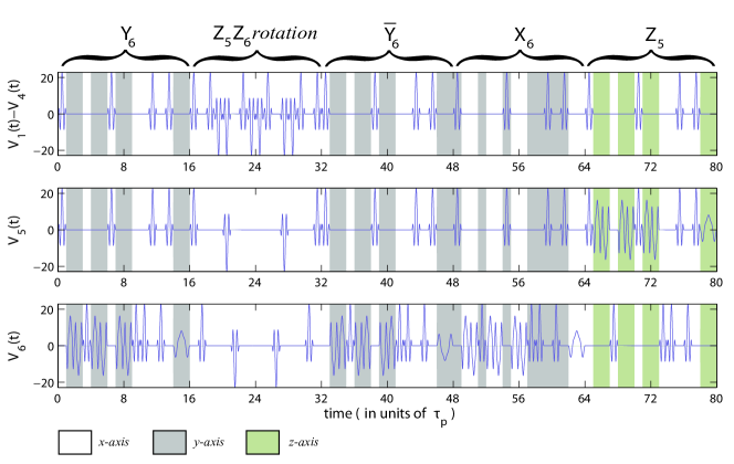
Figure 2: (Color online) Pulse sequences used to implement the CNOT gate between qubits $\mathcal{Q}_{5}$ and $\mathcal{Q}_{6}$ on a star graph. It is a combination of four single-qubit gates ($0<t\leq 16\tau_{p}$, $32\tau_{p}<t\leq 48\tau_{p}$, $48\tau_{p}<t\leq 64\tau_{p}$, and $64\tau_{p}<t\leq 80\tau_{p}$) and a single instance of the $ZZ$-coupling sequence, $16\tau_{p}<t\leq 32\tau_{p}$. For better accuracy this latter sequence has to be repeated several times, we used $N_{\mathrm{rep}}=5$ repetitions, see Ref. De and Pryadko, 2014 for detailed discussion of the associated errors. Second-order self-refocusing pulse shapes $Q_{1}(\pi)$ and $Q_{1}(\pi/2)$ from Refs. Sengupta and Pryadko, 2005; Pryadko and Sengupta, 2008 are used. The shading shows the direction of the applied pulses as indicated.

Two-qubit $ZZ$-rotation gatesDe and Pryadko (2013a, 2014) are designed using a different approach, see Fig. 2. The idea is to selectively decouple some of the inter-qubit interactions, with the needed rotations generated by the residual interactions when the sequence is repeated over some specified amount of time. This only requires conventional decoupling sequences which are, generally, easier to design.

The qubits are divided into four sets: idle qubits on sublattices $A$ and $B$ (depending on the chosen graph), and the sets $A^{\prime}\subseteq A$ and $B^{\prime}\subseteq B$ which together make up all of the pairs of neighboring qubits where we want to preserve the couplings. The corresponding sequences are denoted $V_{A}$, $V_{B}$, $V_{A^{\prime}}$, and $V_{B^{\prime}}$. The universal idle-qubits sequences $V_{A}$ and $V_{B}$ must decouple both the system (2) and the bath (3) Hamiltonians, and have sufficient flexibility so that the coupling with a neighboring opposite-sublattice qubit driven by the sequence $V_{B^{\prime}}$ and $V_{A^{\prime}}$ respectively could also be decoupled. On the other hand, the sequences $V_{A^{\prime}}$ and $V_{B^{\prime}}$ executed on the pairs of qubits to remain coupled must average out the bath Hamiltonians (3), but leave some fraction $f$ of the original coupling (2) between these qubits.

We designed the global sequences $V_{A}$ and $V_{B}$ to allow for construction of local versions of the sequences $V_{B^{\prime}}(f)$ and $V_{A^{\prime}}(f)$, with some range of allowed fractions $f$. This makes the fraction $f$ locally adjustableDe and Pryadko (2014), to accommodate for possible local variations of the couplings $J_{ij}$. In this work we assume all couplings equal (non-zero $J_{ij}=J$ iff the sites $i$ and $j$ are connected), and use the fastest version of these sequences of duration $\tau_{\mathrm{seq}}=16\tau_{p}$ with a fixed fraction $f=1/2$, as used originally in Ref. De and Pryadko, 2013a. Over the duration of the sequence, for each pair of qubits designated to be coupled, the original coupling $J_{ij}\equiv J$ in Eq. (2) is reduced to $fJ=J/2$, which gives the rotation angle $\alpha=fJ\tau_{\mathrm{sec}}/2$.

We constructed a cnot gate using the identityGaliautdinov (2007); Geller et al. (2010)

$$U_{jk}^{(\text{C-}X)} = Y_{j}X_{k}\bar{X}_{j}\bar{Y}_{j}\bar{Y}_{k}\exp\Bigl{(}-i\frac{\pi}{4}\sigma^{z}_{j}\sigma^{z}_{k}\Bigr{)}Y_{k}$$ (6)

$$= Z_{j}X_{k}\bar{Y}_{k}\exp\Bigl{(}-i\frac{\pi}{4}\sigma^{z}_{j}\sigma^{z}_{k}\Bigr{)}Y_{k},$$ (7)

where, e.g., $X_{k}\equiv-i\sigma_{k}^{x}$ and $\bar{X}_{k}\equiv i\sigma_{k}^{x}$ respectively are the unitaries corresponding to $\pm\pi$ rotations of the $k$-th qubit around the $X$ axis. Eq. (7) requires a $ZZ$ rotation with the rotation angle $\alpha=\pi/4$. Thus, the pulse duration $\tau_{p}$ and the number of repetition $N_{\mathrm{rep}}$ must satisfy the design equationDe and Pryadko (2013a)

$$N_{\mathrm{rep}}\,J\tau_{p}=\frac{\pi}{16}.$$ (8)

Larger values of $N_{\rm rep}$ correspond to smaller values of the perturbation-theory parameter $J\tau_{p}$ which improves the fidelity as it provides better decoupling. On the other hand, this also increases the cost in terms of the number of pulses. The actual set of driving fields used to implement the cnot gate with $N_{\rm rep}=1$ are shown in Fig.2. For our calculations we used $N_{\rm rep}=5$.

We also implemented two other controlled two-qubit gates using the identities

$$U_{jk}^{(\text{C-}Y)} = e^{-i\pi/4}\bar{X}_{2}\bar{Z}_{j}\bar{Z}_{k}\exp\Bigl{(}-i\frac{\pi}{4}\sigma^{z}_{j}\sigma^{z}_{k}\Bigr{)}X_{k},$$ (9)

$$U_{jk}^{(\text{C-}Z)} = e^{-i\pi/4}\bar{Z}_{j}\bar{Z}_{k}\exp\Bigl{(}-i\frac{\pi}{4}\sigma^{z}_{j}\sigma^{z}_{k}\Bigr{)},$$ (10)

as well as the swap gate as a sequence of three cnot gates.Barenco et al. (1995)

II.3 Five-qubit code on a star graph

We use the smallest single-error-correcting code Bennett et al. (1996); Calderbank et al. (1997); Laflamme et al. (1996) formally denoted as $[[5,1,3]]$. This distance-three code encodes a single qubit in a two-dimensional subspace $\mathcal{Q}$ of the $2^{5}$-dimensional Hilbert space of $n=5$ qubits. It is a stabilizer codeGottesman (1997): the subspace

$$\mathcal{Q}=\{\left|\psi\right\rangle:\,G_{i}\left|\psi\right\rangle=\left|\psi\right\rangle,\;i=1,2,\ldots r\}$$

is a common $+1$ eigenspace of the $r=4$ independent commuting stabilizer generators,

$$G_{1}=XZZXI\equiv\sigma_{1}^{x}\sigma_{2}^{z}\sigma_{3}^{z}\sigma_{4}^{x},$$ (11)

$$G_{2}=IXZZX\equiv\sigma_{2}^{x}\sigma_{3}^{z}\sigma_{4}^{z}\sigma_{5}^{x},$$

$$G_{3}=XIXZZ\equiv\sigma_{1}^{x}\sigma_{3}^{x}\sigma_{4}^{z}\sigma_{5}^{z},$$

$$G_{4}=ZXIXZ\equiv\sigma_{1}^{z}\sigma_{2}^{x}\sigma_{4}^{x}\sigma_{5}^{z},$$

expressed as Kronecker products of single-qubit Pauli operators $\sigma_{i}^{\mu}$, $\mu=x,y,z$. Notice that to reduce the confusion with the pulse unitaries in Sec. II.2, here we quote both the commonly used positional and the traditional notations for multi-qubit Pauli operators.

As for any stabilizer code, encoding of the five-qubit code can be done efficientlyGottesman (1997). We have used the conceptual encoding circuit in Fig. 3(a), which produces the code in the basis with the logical operators $\bar{X}=-XXXXX$ and $\bar{Z}=ZZZZZ$. This circuit is based on a representation of the five-qubit code as a code word stabilized (CWS) codeCross et al. (2009), and was constructed as a simplification of the circuit containing the Hadamard gate on the information qubit, encoder for the classical five-qubit repetition code, and the graph state encoderRaussendorf et al. (2003). Explicitly, the resulting basis wavefunctions corresponding to the eigenvalues $\lambda_{\bar{Z}}=(-1)^{m}$, $m=0,1$, are (up to a normalization)

$$\left|\Psi_{m}\right\rangle = \left|0000m\right\rangle-\left|0110m\right\rangle+\left|1001m\right\rangle-\left|1111m\right\rangle$$

$$+ \left|0010\bar{m}\right\rangle+\left|0100\bar{m}\right\rangle-\left|1101\bar{m}\right\rangle-\left|1011\bar{m}\right\rangle$$

$$-(-)^{m} \!\times \!\!\bigl{(}\left|0001\bar{m}\right\rangle+\left|1110\bar{m}\right\rangle+\left|0111\bar{m}\right\rangle+\left|1000\bar{m}\right\rangle$$ (12)

$$+ \left|0011m\right\rangle-\left|0101m\right\rangle-\left|1010m\right\rangle+\left|1100m\right\rangle\bigr{)}.\qquad$$

(a)              
(b)

Figure 3: (a) Conceptual encoding circuit for the [[5,1,3]] code using the Hadamard, cnot, and controlled-phase gates. On the input, the first four qubits are initialized in $\left|0\right\rangle$ states and the last qubit contains the state $\left|\psi\right\rangle\equiv\alpha\left|0\right\rangle+\beta\left|1\right\rangle$ to be encoded. On the output, the corresponding logical state $\alpha\left|\bar{0}\right\rangle+\beta\left|\bar{1}\right\rangle$ of the five-qubit code is produced. The decoding is done by inverting the encoding circuit. (b) Actual encoding circuit implemented on a six-qubit star graph. Two swap operations are required since qubits on the leaves can only interact with the qubit $6$ in the center. In addition, the ancilla qubit is swapped to the center at the end to prepare for the measurement cycle, see Fig. 4.

To implement the same circuit on the star graph, we used two more swap operations, plus an additional swap at the end to place the ancilla at the center, see Fig. 3(b). This initializes for the stabilizer generator measurement cycle shown in Fig. 4.

Figure 4: The circuit for a single cycle of measuring the stabilizer generators (11) for the five-qubit code on a star graph. On the input and the output, the first five qubits contain an encoded state. The same ancilla qubit $6$ at the center is used for each measurement; $M$ stands for measurement and resetting to $\left|0\right\rangle$ if needed. We implemented this circuit which uses 16 cnot gates (duration $144\tau_{p}$ each) and 8 rounds of Hadamard gates (duration $32\tau_{p}$ each) applied in parallel, with the total measurement cycle duration of $2560\tau_{p}$ ($640\tau_{p}$ per stabilizer generator). In our simulations, the entire cycle is repeated several times for repetitive QEC.

III Simulations

We implemented the described encoding/decoding and the measurement circuits at the Hamiltonian level, using pulse sequences described in Sec. II.2, and classical zero-mean Gaussian phase noise with Gaussian correlations,

$$\langle A_{i}(t)\rangle=0,\quad\langle A_{i}(t)A_{j}(t^{\prime})\rangle=\sigma^{2}\delta_{ij}e^{-(t-t^{\prime})^{2}/\tau_{n}^{2}},$$ (13)

as a source of decoherence, cf. Eq. (3). Notice that for a single uncontrolled qubit, such a field would produce asymptotic dephasing rate $1/T_{2}=(\sqrt{\pi}/2)\,\sigma^{2}\tau_{n}$.

The corresponding many-body unitary dynamics has been simulated with a C++ program using the Eigen3 libraryGuennebaud et al. (2010) for matrix algebra. The program uses a custom-built algorithm to schedule the pulse sequences and measurement events, and the fourth-order Runge-Kutta algorithm for explicitly integrating the time dependent Schrödinger equation for the unitary time evolution of clusters of multiple qubits. In all simulations shown we used 1024 time steps per nominal pulse duration $\tau_{p}$, resulting in relative integration errors better than $10^{-9}$, comparable to numerical precision.

III.1 Quantum error detection mode

We first consider the working of the [[5,1,3]] code in the error detection mode (quantum Zeno cycleFacchi and Pascazio (2002); Facchi et al. (2002)). In an actual experiment, one is supposed to measure the stabilizer generators repeatedly, with the experiment terminated once an error is detected as indicated by a non-zero syndrome bit. In our simulations, instead, each syndrome measurement was replaced by an instantaneous projection

$$P_{0}\equiv(\openone+\sigma_{6}^{z})/2,$$ (14)

which selects the many-body sector with the ancilla qubit $Q_{6}$ at the center in the state $\left|0\right\rangle$. The success probability averaged over the initial state $\left|\psi\right\rangle$ was calculated according to the expression

$$p_{0}\equiv\mathop{\rm Tr}(U\rho_{0}U^{\dagger}P_{0}),$$ (15)

where $U$ is the $N\times N$ unitary evolution matrix up to the moment of measurement, $\rho_{0}=M^{-1}P_{M}$ is the density matrix describing the uniform distribution of the initial wavefunctions in a subspace of dimensionality $M$, and $P_{M}$ is the corresponding projector. In our simulations, $N=64$ is the dimensionality of the six-qubit Hilbert space, and we compute a reduced $N\times M$ evolution matrix $V$ which include only $M=2$ columns corresponding to the number of basis states of the initial qubit, see the encoding circuit in Fig. 3. Respectively, we used Eq. (15) in the form

$$p_{0}={1\over 2}\mathop{\rm Tr}(V^{\dagger}P_{0}V).$$ (16)

Given the reduced evolution matrix $V\equiv V(t)$ at a given time moment $t$, and the corresponding ideal evolution matrix $V_{0}$, the overall fidelity averaged over the initial state can be calculated using the expression

$$F\equiv F(V,V_{0})={\mathop{\rm Tr}(V_{0}^{\dagger}VV^{\dagger}V_{0})+|\mathop{\rm Tr}(V_{0}^{\dagger}V)|^{2}\over M(M+1)}.$$ (17)

The derivation is similar to that given in the Appendix of Ref. Pryadko and Sengupta, 2008 for the case of $M=N$.

Results of simulations for several sets of parameters of the Gaussian noise, the r.m.s. amplitude $\sigma$ and the correlation time $\tau_{n}$, are shown in Fig. 5. Each plot is an average over 20 instances of the stochastic noise, with the time axis starting at the first measurement after the end of the encoding. Having in mind an experiment where the success probability and the state fidelity would be measured separately, and to match the quantities computed in Ref. De and Pryadko, 2013a, we plot the success probability (SP), and the fidelity “with measurements” (WM) conditioned on the error-free syndrome measurements, $F_{\mathrm{succ}}=F/p_{0}$, where $p_{0}$ is given by Eq. (16). Notice that this expression is an approximation which ignores possible correlations between $p_{0}$ and $F_{\mathrm{succ}}$. These correlations would be absent with ideal syndrome measurements; we expect them to be small in our case since the measurement fidelity is high. The effect of such correlations is additionally suppressed since $F_{\mathrm{succ}}$ is numerically close to one.

To compare the contributions of the DD protection and of the projective measurements (Zeno cycle) to the overall fidelity, in Fig. 5 we also show the average fidelity (17) calculated when decoupling pulses are applied but “no measurements” are done (NM), and when no projective measurements and “no pulses” are applied (NP). Since they involve no projective measurements, these quantities are independent of the success probability (15). For each version of the cycle, filled symbols show the infidelities $1-F$ after each syndrome measurement, while open symbols show the corresponding infidelities to the end of the final decoding. Notice that thus computed fidelities involve all six qubits; final infidelities could be additionally reduced by tracing out all but one information qubit, see Sec. III.2.

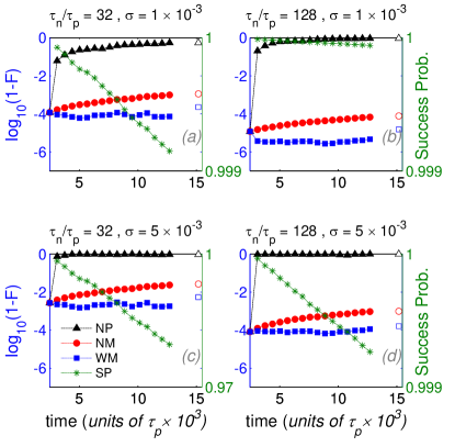
Figure 5: (color online) Infidelities during the Zeno cycle for different noise correlation times and noise amplitudes as indicated. The time axis starts after the completion of the encoding circuit, at the instance of the first measurement, see Figs. 3(b) and 4. The different curves correspond to cases where no pulses are applied (NP), DD pulses are applied but no measurements are done (NM), and with the syndrome measurements (WM). Closed and open symbols respectively represent the infidelities at the end of each syndrome measurement and at the end of the final decoding. Note that the axis for the cumulative success probability (SP) is on the right.

These plots show about an order of magnitude infidelity reduction due to QEC during the cycle. The code can detect any one- and two-qubit error, and a small fraction of higher-weight errors. The fact that the Zeno cycle works, indicates that errors seen by the code are not dominated by multi-qubit correlations. In addition, the infidelities increase sharply with shorter noise correlation times, as expected due to the asymmetry of the single-qubit gates, see Sec. II.2.

Two of the plots shown have exactly the same noise parameters and use the same pulse shapes as in our earlier workDe and Pryadko (2013a) where Zeno cycle was simulated with the $[[4,2,2]]$ error-detecting code, with five qubits arranged in a chain. The corresponding success probabilities and state fidelities are similar in magnitude. We believe this to be a combined result of an improvement due to more efficient code and faster syndrome measurements in the present case, negated by increased errors due to larger connectivity of the star graph, as discussed in detail in Ref. De and Pryadko, 2014.

III.2 QEC mode

In this mode we simulated projective measurements of the ancilla by applying instantaneous projection operators $P_{0}$ [Eq. (14)] or $P_{1}\equiv\openone-P_{0}$. These are six-qubit projectors selecting the sector with the ancilla qubit $Q_{6}$ at the center in the state $\left|0\right\rangle$ or $\left|1\right\rangle$, respectively. Given the normalized wavefunction $\Psi$ of the system, the projectors should be chosen with the probabilities $p_{0}\equiv\left\langle\Psi\right|P_{0}\left|\Psi\right\rangle$ and $p_{1}\equiv\left\langle\Psi\right|P_{1}\left|\Psi\right\rangle=1-p_{0}$, respectively. This implies a separate simulation would be needed for every state $\psi$ of the initial qubit (see the encoding circuit in Fig. 3). Instead, to speed up the simulations, we calculated the reduced unitary evolution matrix $V$ and used the probability (16) averaged over the initial state of the qubit. The normalization of $V$ was corrected after each projection. This approximation is similar to that used in the previous section to define the fidelity $F_{\mathrm{succ}}$ conditioned on the string of zero-syndrome measurements in each previous cycle. Here, we also expect the effect of any potential unaccounted correlations to be suppressed due to the smallness of $p_{1}=1-p_{0}$.

As in the previous section, we simulated decoherence with classical phase noise applied on all six qubits involved in the simulations. The noise was uncorrelated between different qubits. For each qubit, the noise was generated as a stationary zero-mean Gaussian stochastic process with Gaussian time correlations. Individual traces of such simulations for three realizations of the Gaussian stochastic noise with identical correlation time $\tau_{n}=32\tau_{p}$ and different r.m.s. amplitudes as indicated are shown in Fig. 6. Each panel shows four different infidelity measures $1-F$ computed during a single simulation run. The fidelities $F_{\mathrm{b}}$ and $F_{\mathrm{a}}$ are computed according to Eq. (17), respectively, just before and right after each projective measurement. The fidelities $F_{\mathrm{b}}^{\prime}$ and $F_{\mathrm{a}}^{\prime}$ computed at the same time moments include idealized recovery channel, see Eq. (18) and the discussion below.

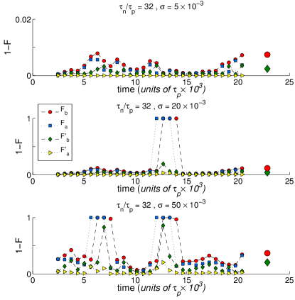
Figure 6: Sample error correction traces for $[[5,1,3]]$ code in the presence of the stochastic phase noise on all six qubits. The noise correlation time is $\tau_{n}=32\tau_{p}$ and noise amplitudes $\sigma$ are as indicated (in units $\tau_{p}^{-1}$). Plots show different infidelity measures $1-F$ during the stabilizer measurement cycle and at the end of the decoding. Here $F_{\mathrm{b}}$ and $F_{\mathrm{a}}$ are the regular fidelities [Eq. (17)], respectively, computed just before and right after each projective measurement. $F^{\prime}_{\mathrm{b}}$ and $F^{\prime}_{\mathrm{a}}$ are the corresponding fidelities which include idealized recovery for single qubit errors, see Eq. (18). Larger symbols indicate the infidelities at the end of the decoding circuit, where the circle corresponds to the full-system fidelity (17), and the diamond to the single-qubit fidelity after tracing out the qubits away from the center.

The five-qubit code is a “perfect” single-error-correcting code, since the fifteen ($2^{4}-1$) non-zero syndromes corresponding to four stabilizer generators (11) are in a one-to-one correspondence with the fifteen single-qubit errors. We used this idealized map for decoding. Notice, however, that in our simulations the stabilizer generators are measured sequentially, with the entire measurement cycle typically repeated just a few times. To increase the syndrome measurement fidelity, we did not adhere to a fixed measurement cycle and instead triggered the beginning of a cycle by a syndrome measurement returning a non-zero bit. After the fourth measurement, the correction would be computed and applied immediately. Typically, the infidelities $1-F_{\mathrm{b}}$ computed right before a trigger event were small, whereas right after the infidelity $1-F_{\mathrm{a}}$ jumps to near one, as the wavefunction is projected outside of the code. The infidelities $1-F_{\mathrm{b}}$ remain large right before the subsequent three measurements, creating an easy to spot four-dot pedestal in the combined trace. For example, no trigger events happened in the top trace in Fig. 6 ($\sigma=5\times 10^{-3}/\tau_{p}$), one happened in the middle trace ($\sigma=20\times 10^{-3}/\tau_{p}$), and two in the bottom trace ($\sigma=50\times 10^{-3}/\tau_{p}$).

To look beyond the simple system fidelity (17), we also calculated the fidelity including the idealized recovery map,

$$F^{\prime}(V,V_{0})=F(V,V_{0})+\sum_{i=1}^{15}F(V,E_{i}V_{0}),$$ (18)

where $E_{i}$, $i=1,\ldots,15$, are all single-qubit errors on the peripheral qubits, and $F(V,V_{0})$ is the usual fidelity (17). This expression corresponds to idealized error correction, with the summation over all single-qubit errors corresponding to that over all possible syndromes.

We should mention that in our calculations both fidelity expressions include the ancilla qubit which has not been traced out. However, since the ancilla is reset to $\left|0\right\rangle$ state after each projective measurement, it is effectively excluded for the fidelities $F_{\mathrm{a}}$ and $F_{\mathrm{a}}^{\prime}$ computed right after the measurement. The ancilla is also included in the full-system fidelity $F$ computed at the end of the decoding circuit, but not in the final fidelity $F^{\prime}$ which only looks at the state of the single qubit in the center. In our plots these fidelities are shown with bigger symbols.

The plots in Fig. 6 show the simulated infidelities for one simulation run each, they are strongly affected by the details of the particular noise realization and the measurement results simulated probabilistically. In Fig. 7 we show (in the logarithmic scale) infidelities averaged over 25 different realizations of the stochastic noise. To reduce the unphysical fluctuations, large infidelities after the trigger events have been excluded from the averages.

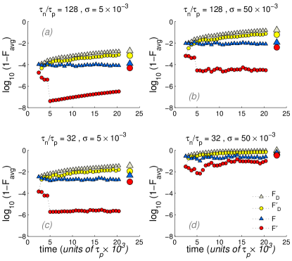
Figure 7: Infidelities $1-F$ for the $[[5,1,3]]$ code averaged over 25 realizations of the stochastic Gaussian noise, with the noise correlation times $\tau_{n}$ and amplitudes $\sigma$ as indicated. Large infidelities after trigger events have been excluded from the averages. $F$ are the regular fidelities [Eq. (17)] computed right after each projective measurement, $F^{\prime}$ are the corresponding fidelities which include idealized recovery for single qubit errors, see Eq. (18). In addition $F_{D}$ and $F^{\prime}_{D}$, respectively, are the fidelities (17) and (18) for DD-only simulations with the same pulse sequences run but error correction turned off (no projective measurements). Larger symbols indicate the respective quantities at the end of the decoding circuits, with $F^{\prime}$ and $F_{D}^{\prime}$ replaced by the average single-qubit decoded fidelities, with the qubits away from the center traced out.

The data in Fig. 7 also include average infidelities $1-F_{D}$ and $1-F_{D}^{\prime}$ [Eqs. (17) and (18)] produced in identical simulations but with error correction turned off (the same pulse sequences but no projective measurement). Except for the plots in Fig. 7(d), where QEC becomes relatively ineffective due to strong noise with shorter correlation time, the DD-only infidelities show a substantially steeper growth than those where both DD and QEC was active. The overall QEC effectiveness can be quantified by comparing the final single-qubit infidelities $1-F_{D}^{\prime}$ and $1-F^{\prime}$ at the end of the decoding (two larger circles). The corresponding ratios of average infidelities for different panels in Fig. 7 are: (a) $14.3$, (b) $15.0$, (c) $9.73$, and (d) $1.36$. Except for the data in Fig. 7(d), QEC in these plots gives average infidelity reduction by an order of magnitude or better. Notice that for this data, trigger events are rare; here QEC fidelity is similar to that for the Zeno cycle, see Sec. III.1.

In the three plots where QEC works well, Fig. 7(a)–(c), the data for $1-F^{\prime}$ is some two orders of magnitude below that for $1-F$, indicating that in the present setup single-qubit errors strongly dominate. This is in an apparent contrast with the results of our Ref. De and Pryadko, 2014, where we concluded that multi-qubit errors are an unavoidable feature of the perturbatively designed gates. We notice, however, that due to asymmetry of single-qubit gates, in the presence of time-dependent noise, the leading-order error terms are single-qubit Pauli operatorsDe and Pryadko (2014), with the coefficients scaling as a derivative of the classical fields $A_{i}(t)$. Further correlated errors are formed in higher orders of the Magnus series, they can be represented as connected clusters on the connectivity graph. On the star graph, these include a single bond joining the ancilla at the center to one of the code qubits, and, in the next order, two bonds, which could result in a correlated error involving the ancilla and two qubits of the code. Thus, after the ancilla is projected during the measurement, the remaining errors on the qubits forming the code are expected to have smaller weight than they would with a different connectivity graph. The applicability of these arguments is improved by our choice $N_{\mathrm{rep}}=5$, which gives the perturbation theory parameter $J\tau_{\mathrm{sec}}=\pi/5$, where $\tau_{\mathrm{sec}}=16\tau_{p}$ is the typical sequence duration, see Eq. (8).

This analysis is confirmed by the plots in Fig. 8, which show infidelity traces for different amplitudes of the noise with the correlation time $\tau_{n}=128\tau_{p}$. The two top panels, with noise amplitudes $\sigma=0$ and $\sigma=5\times 10^{-3}/\tau_{p}$, show near identical plots for $F^{\prime}$, indicating that with the noise parameters as in Fig. 8(b), multi-qubit errors are strongly dominated by the systematic errors due to the couplings $J$. At the same time, single-qubit errors are dominated by the stochastic noise, since at $\sigma=0$, the plots for $F$ and $F^{\prime}$ fall nearly on top of each other.

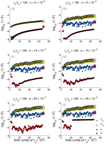
Figure 8: As in Fig. 6 but with longer noise correlation time, $\tau_{n}=128\tau_{p}$. Different infidelities are labeled as in Fig. 7.

Similar conclusions can be also drawn from the data in Fig. 9, which shows the effect of a much faster noise, with the correlation time $\tau_{n}=\tau_{p}$. Namely, the infidelities in Fig. 9(a) were generated by averaging the results of 25 simulations with different realizations of Gaussian noise with the correlation time $\tau_{n}=128\tau_{p}$, while the noise for infidelities in Fig. 9(b), in addition, also included weaker but faster-varying noise components with $\tau_{n}=\tau_{p}$. Dynamical decoupling has nearly no effect on such a fast noise. Respectively, the usual infidelity $1-F$ increased by an order of magnitude, while the infidelity $1-F^{\prime}$ including idealized recovery map [see Eq. (18)] increased by more than two orders of magnitude. Such a different scaling of the two infidelities dominated by one- and multi-qubit errors, respectively, is consistent with the expectation of the absence of DD protection against the faster noise. Quantitatively, the ratios of the final average single-qubit infidelities at the end of the decoding in runs with and without error correction are 15.7 in Fig. 8(a) and 8.0 in Fig. 8(b).

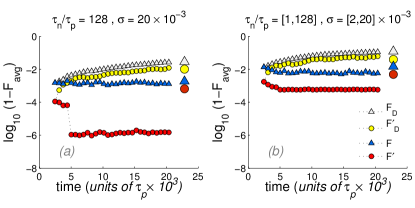
Figure 9: As in Fig. 7, comparing the effect of fast dephasing noise. The plots at the left show infidelities averaged over 25 realizations of a Gaussian stochastic noise with r.m.s. amplitude $\sigma=20\times 10^{-3}/\tau_{p}$ and $\tau_{n}=128\tau_{p}$. For the data on the right, in addition, there was also a weak noise with $\sigma=2\times 10^{-3}/\tau_{p}$ and a much shorter correlation time $\tau_{n}=\tau_{p}$. Such a noise is not affected by the DD. With the addition of the fast noise, the infidelity $1-F$ increased by about an order of magnitude, while the infidelity $1-F^{\prime}$ accounting by multi-qubit errors increased by two orders of magnitude, consistent with the expected absence of DD protection against the fast noise component.

IV Discussion

For many years, the road to building a quantum computer appeared to be straightforward: one just had to manufacture a sufficient number of quality qubits and implement a universal set of quantum gates of sufficiently high fidelity. Now that we are there, or nearly there, it turns out that fidelity is not the ultimate measure of performance in large qubit systems. As the number of qubits in a quantum computer grows, exponentially so does the number of ways it can go wrong. To understand what is going on in a particular implementation of a quantum computer would require detailed numerical simulations, including as many qubits and as much physical detail as possible.

In this work we presented one such simulation, implementing repetitive QEC with the $[[5,1,3]]$ code on a six-qubit network with always-on Ising couplings and classical correlated phase noise as a source of decoherence. The one- and two-qubit gates were implemented via carefully designed sequences of shaped pulses. Realistically simulating such gates and associated errors requires integrating the corresponding multi-qubit unitary dynamics. Such simulations, like current experiments, are limited to very small system sizes. As a result, one can use only simplest weak codes, with very few ancillary qubits, which puts additional constraints on the accuracy of the implemented gates.

As in any case where gates are designed perturbatively, up to some fixed order in the perturbation (interaction) Hamiltonian, the systematic errors associated with our gates are correlated multi-qubit errors, which worsen with the increased connectivity of the qubit network. On the other hand, the $[[5,1,3]]$ code we used is able to correct only single-qubit errors. To make QEC possible, we had to tune the couplings down and make the two-qubit gates longer, increasing the intrinsic fidelities of our gates to six nines or more. As a result, just a few rounds of repetitive QEC required tens of thousands of pulses, with the fidelity noticeably suffering, e.g., from relatively modest integration errors (not shown). In this weakly coupled regime, our simulations show that single-qubit errors due to phase noise do not propagate excessively.

Overall, we demonstrated repetitive quantum error correction in a fully quantum-mechanical simulation, with the error correction responsible for the average infidelity reduction by an order of magnitude or more. We have also presented a combined protocol integrating dynamical decoupling and quantum error correction. Dynamical decoupling is particularly effective against low-frequency noise which in our simulations had an asymptotic dephasing time $T_{2}$ as short as few nominal pulse lengths $\tau_{p}$. We also saw that our combined DD/QEC protocol remains effective in the presence of a weak high-frequency phase noise.

While dephasing-only model appear to be too simplistic, we notice that as a result of controlled dynamics, some of the dephasing propagates to the longitudinal channelPryadko and Quiroz (2009). In particular, our original simulations which involved similar gates with the three-qubit code protecting against single-qubit phase errors, produced a much smaller fidelity improvement due to QECDe and Pryadko (2013b).

Our model excludes many physical effects which may be relevant for engineering a quantum computer based on a specific qubits implementation, such as couplings between nominally disconnected qubits, multi-level structure of the solid-state qubits and corresponding leakage errors, violations of the rotating wave approximation, realistic decoherence which may produce additional correlations between the qubits, etc. Even when the corresponding effects are small, they can result in errors correlated in time or between qubits, and thus strongly affect the overall coherent multi-qubit dynamics. Designing coherence protection schemes with improved stability against such effects is also possible, if one knows which decoherence mechanisms are dominant. Each additional improvement would require more finely tuned pulse shapes, longer gates, or a longer code, increasing the requirements on the dynamical range of the qubit system used in the experiment. Thus, in our opinion, careful studies of realistic models which incorporate such effects are absolutely necessary in order to construct a scalable quantum computer.