The $Caterpillar$ Project: A Large Suite of Milky Way Sized Halos

Abstract

We present the largest number of Milky Way sized dark matter halos simulated at very high mass ($\sim$ $10^{4}$ $\mathrm{M_{\sun}}$/particle) and temporal resolution (5 Myrs/snapshot) done to date, quadrupling what is currently available in the literature. This initial suite consists of the first 24 halos of the Caterpillar Project whose project goal of 60 – 70 halos will be made public when complete. We do not bias our halo selection by the size of the Lagrangian volume. We resolve $\sim$20,000 gravitationally bound subhalos within the virial radius of each host halo. Improvements were made upon current state-of-the-art halo finders to better identify substructure at such high resolutions, and on average we recover $\sim$4 subhalos in each host halo above 10⁸ $\mathrm{M_{\sun}}$ which would have otherwise not been found. The density profiles of relaxed host halos are reasonably fit by Einasto profiles ($\alpha$ = 0.169 $\pm$ 0.023) with dependence on the assembly history of a given halo. Averaging over all halos, the substructure mass fraction is $f_{m,subs}=0.121\pm 0.041$, and mass function slope is d$N$/d$M\propto M^{-1.88\pm 0.10}$. We find concentration-dependent scatter in the normalizations at fixed halo mass. Our detailed contamination study of 264 low-resolution halos has resulted in unprecedentedly large high-resolution regions around our host halos for our fiducial resolution (sphere of radius $\sim 1.4\pm 0.4$ Mpc). This suite will allow detailed studies of low mass dwarf galaxies out to large galactocentric radii and the very first stellar systems at high redshift ($z$ $\geq$ 15).

1. Introduction

Under the current paradigm of structure formation (White & Rees, 1978) stellar halos of large galaxies such as the Milky Way are believed to be primarily formed as a result of the accumulation of tidal debris associated with ancient as well as recent and ongoing accretion events (Helmi 2008, Pillepich et al. 2015). In principle, the entire merger and star formation history of our Galaxy and its satellites can be probed with their stellar contents (i.e., the “fossil record”; Freeman & Bland-Hawthorn 2002) because this information is not only encoded in the dynamical distribution of the different Galactic components, but also in the stellar chemical abundance patterns (e.g., Font et al. 2006; Gómez et al. 2010).

To further map out the structure and composition of the various components of the Milky Way, large scale observational efforts are now underway. Several surveys such as rave (Steinmetz et al., 2006), segue (Yanny et al., 2009), apogee (Majewski et al., 2010), lamost (Deng et al., 2012) and galah (Freeman, 2012) have collected medium-resolution spectroscopic data on some four million stars primarily in the Galactic disk and stellar halo. There are also ongoing large-scale photometric surveys such as Pan-STARRS (Kaiser et al., 2010) and SkyMapper Southern Sky Survey (Keller et al., 2013) mapping nearly the entire sky. Soon, the gaia satellite (Perryman et al., 2001) will provide precise photometry and astrometry for another one billion stars.

Studies of individual metal-poor halo stars have long been used to establish properties of the Galactic halo, such as the metallicity distribution function, to learn about its history and evolution. More recently, the discoveries of the ultra-faint dwarf galaxies (with $L_{\rm tot}\leq 10^{5}\,L_{\odot}$) in the northern Sloan Digital Sky Survey (SDSS) and the southern Dark Energy Survey (DES) have shown them to be extremely metal-deficient systems which lack metal-rich stars with ${\rm[Fe/H]\gtrsim-1.0}$. To some extent they can be considered counterparts to the most metal-poor halo stars. They extend the metallicity-luminosity relationship of the classical dwarf spheroidal galaxies down to $L_{\rm tot}\sim 10^{3}\,L_{\odot}$ (Kirby et al., 2008), and due to their relatively simple nature, they retain signatures of the earliest stages of chemical enrichment in their stellar population(s). Indeed, the chemical abundances of individual stars in the faintest galaxies suggest a close connection to metal-poor halo stars in the Galaxy (Frebel & Norris, 2015).

This comes at a time when there is still uncertainty over what role dwarf galaxies play in the assembly of old stellar halos because the true nature of the building blocks of large galaxies (e.g., Helmi & de Zeeuw 2000, Johnston et al. 2008, Gómez et al. 2010) are not yet fully understood. Nevertheless, observations of the, e.g., the Segue 1 ultra-faint dwarf suggest that these faintest satellites could be some of the the universe’s first galaxies (presumably the building blocks) that survived until today (Frebel & Bromm, 2012; Frebel et al., 2014). They would thus be responsible for the Milky Way’s oldest and most metal-poor stars.

This wealth of observational results offers unique opportunities to study galaxy assembly and evolution and will thus strongly inform our understanding of the formation of the Milky Way. Along with it, the current dark energy plus cold dark matter paradigm ($\Lambda$CDM) can be tested at the scales of the Milky Way and within the Local Group. But to fully unravel the Galaxy’s past and properties, theoretical and statistical tools need to be in place to make efficient use of data.

For over three decades now, numerical simulations of structure formation have consistently increased in precision and physical realism (see Somerville & Davé 2014 for a review). Originally, they began as a way to study the evolution of simple N-body systems (e.g., merging galaxies; Aarseth 1963, Toomre & Toomre 1972, White 1978 and globular clusters; Hénon 1961) but with the advent of better processing power and more sophisticated codes (e.g., Springel 2010, Hopkins 2015, Bryan et al. 2014), N-body solvers are now fully coupled to hydrodynamic solvers allowing for a comprehensive treatment of the evolution of the visible Universe (e.g., Vogelsberger et al. 2014, Schaye et al. 2015).

The most efficient method of studying volumes comparable to the Local Group whilst maintaining accurate large scale, low-frequency cosmological modes is via the zoom-in technique (Katz et al. 1994, Navarro & White 1994). This technique allows one to efficiently model a limited volume of the Universe at an extremely high resolution. Owing to the extreme dynamic range offered by such simulations, both the inside of extremely low mass, gravitationally bound satellite systems can be studied along side the hierarchical assembly of their host galaxy (e.g., Stadel et al. 2009). Gravity solvers which use hybrid tree-particle-mesh techniques (e.g., Gadget-2, Springel 2005) are ideally suited to carrying out such calculations on these scales. In addition to tailored codes for studying Milky Way sized halos, halo finders used for identifying substructure contained within them have also drastically improved over the past 30 years. Simple friends-of-friends (FoF) algorithms (e.g., Davis et al. 1985) have now evolved into parallel, fully hierarchical FoFs algorithms adopting six phase-space dimensions and one time dimension allowing shape-independent, and noise-reduced identification of substructure (Behroozi et al. 2013). These tools are very robust methods for accurately identifying bound substructures (e.g., Onions et al. 2012), though Behroozi et al. (2015) has recently highlighted the difficulty in connecting halos during merger events. These efforts demonstrate that only algorithms that combine phase-space and temporal information should be used.

Two primary groups have performed zoom-in N-body simulations of the growth of Milky Way sized halos in extremely high resolution – the Aquarius project of Springel et al. (2008) and the Via Lactea simulations of Diemand et al. (2008). Whilst these works have been thoroughly successful and made it possible to quantify the formation of the stellar halo, for example, both the Aquarius and Via Lactea projects are limited in a number of respects.

The first of these is that they adopted the now observationally disfavored Wilkinson Microwave Anisotropy Probe’s first set of cosmological parameters (WMAP-1, Spergel et al. 2003). The advent of the Planck satellite (Planck Planck Collaboration et al. 2014) with three times higher resolution and better treatment of the astrophysical foreground (owing in large part to using nine frequency bands instead of five with WMAP) has allowed even more precise estimates of key cosmological parameters. In particular, the most crucial of these for accurate cosmological simulations are the baryon density ($\Omega_{b}$), the matter density ($\Omega_{c}$), the dark energy density ($\Omega_{\Lambda}$), the density fluctuations at 8 $h^{-1}$ Mpc ($\sigma_{8}$) and the scalar spectral index ($n_{s}$). Dooley et al. (2014) showed through a systematic studies of structure formation using different cosmologies that the maximum circular velocities, formation and accretion times of a given host’s substructure are noticeably different between cosmologies. $\sigma_{8}$ in WMAP-1 for example is much higher ($\sigma_{8,WMAP1}$ = 0.9 vs. $\sigma_{8,Planck}$ = 0.83) which shifts the peak in cosmic star formation rate to lower redshift, resulting in slightly bluer galaxies at z = 0 (Jarosik et al. 2011, Guo et al. 2013, Larson et al. 2015).

The second major drawback and perhaps more significant is that the Aquarius and Via Lactea simulations were simply limited in number. The Aquarius project consists of six well-resolved Milky Way mass halos, while the Via Lactea study focused on only one such halo.

There exists significant halo-to-halo scatter in, e.g., the substructure shape and abundance owing to variations in accretion history and environment, (Springel et al. 2008, Cooper et al. 2010, Boylan-Kolchin et al. 2010), with the dispersion appearing significant (a factor $>3$, Lunnan et al. 2012). But based on such a small sample, the extent cannot be well-quantified, although determining the distributions of substructure properties of galaxy halos is critical for interpreting the various observations of dwarf galaxy populations of all large galaxies, including the Milky Way and Andromeda.

More recently, Garrison-Kimmel et al. (2014b) have produced a suite of 36 Milky Way halos (24 isolated analogues, 12 Local Group analogues; ELVIS suite) at a resolution of $\sim$$10^{5}$ $M_{\sun}$ per particle ($\sim$Aquarius level-3). Studies using this suite have again highlighted the case for the too big to fail problem (Boylan-Kolchin et al. 2011) by showing that the so called “massive failures” (i.e. halos with $V_{\mathrm{max}}$ $\geq$ 25 km s^-1 that became massive enough to have formed stars in the presence of an ionizing background, $V_{\mathrm{peak}}$ $\geq$ 30 km s^-1) do not disappear when larger numbers of halos across a range of host masses are simulated (Garrison-Kimmel et al., 2014b). Despite the ELVIS suite’s utility, it unfortunately lacks the extra mass resolution required to study the formation of minihalos and very small dwarf galaxies ($\sim 10^{6}$ M_⊙), both at the present day and their evolution since the epoch of reionization. Also, ELVIS is not suitable for using the particle tagging technique whereby a few per cent of the central dark matter particles of accreting systems are assigned stellar properties to study the assembly of the stellar halo (e.g., Cooper et al. 2015). If we are to understand the origin of the first stellar systems (including their chemical constituents) and to locate their descendants at the present day, higher resolution as well as particle tagging is of critical importance.

Whilst previous simulations all have their own merits and drawbacks, one issue prevalent across nearly all previous studies is that they introduced bias in selecting their halos. Usually halo candidates studied using the zoom-in technique meet three criteria: isolation, merger history and Lagrangian volume. From a computational standpoint, if one can obtain a compact Lagrangian region, a quiet merger history and keep the halo relatively isolated, the savings in CPU-hours can be immense. Ultimately, however this three-pronged approach introduces a selection bias. Whilst constructing a simulation with these three key criteria in place will generate an approximate Milky Way analogue, one will not gain an understanding of how the results from studying this halo will compare to halos more generally selected from a pool in the desired mass range (e.g., 1 – 2 $\times$ $10^{12}$ $\mathrm{M_{\sun}}$).

The first requirement is that the halos have a quiescent merger history, which is usually defined by the host having no major merger since a given redshift, e.g., z = 1 (e.g., Springel et al. 2008). Constraining the merger history of a simulation suite severely limits the capabilities of reconstructing the formation history of the Milky Way. Indeed, by statistically contrasting observational data sets to mock data extracted from a set of Milky Way-like dark matter halos, coupled to a semi-analytical model of Galaxy formation (Tumlinson, 2009), Gómez et al. (2012) showed the best-fitting input parameter selection strongly depends on the underlying merger history of the Milky Way-like galaxy. For example, even though for every dark matter halo it is always possible to find a best-fitting model that tightly reproduces the Milky Way satellite luminosity function, these best-fitting models generally fail to reproduce a second and independent set of observables (see Gómez et al. 2014). It is thus critical to sample a wide range of evolutionary histories. The second requirement that the Lagrangian volume of the halo’s particles be compact also in part biases the merger history of the halo. For a fixed z = 0 virial mass, the smaller the Lagrangian volume of a halo, the less likely that halo will have a late major-merger event. This bias further compounds the aforementioned issues of selecting halos with quiet merger histories. Lastly, the isolation criteria preferentially selects halos in low density environments, resulting in decreased substructure (Ragone-Figueroa & Plionis, 2007) and higher angular momentum (Avila-Reese et al. 2005, Lee 2006).

In light of all of these issues, we are motivated to create a comprehensive dataset consisting of 60–70 dark matter halos of approximately Milky Way mass in extremely high spatial and temporal resolution with a more relaxed selection criteria to not just understand the origin and evolution of the Milky Way, but additionally how it differs to other galaxies of similar mass in general. Moreover, this new simulation set (unlike the $Aquarius$ and $Via$ $Lactea$ which were very specific in nature) lends itself well to studying the substructure and stellar halos of $\sim$10¹² $\mathrm{M_{\sun}}$ galaxies such as those being studied in the recently completed ghosts survey (de Jong et al., 2007; Monachesi et al., 2013, 2015).

We call this simulation suite The Caterpillar Project owing to the similarity between each of the individual halos and how they work together towards a common purpose. Due to the extreme computational requirement for a project of this size ($\sim$14M CPU hours and $\sim$700TB of storage), we are staggering our release. For this first paper, we focus on the general $z$ = 0 properties of the first 24 halos of the Caterpillar suite in order to clearly demonstrate data integrity and utility. In Section 2, we outline the simulation suite parameters, numerical techniques, and halo properties. In Section 3 we present a variety of initial results drawn from the suite. In Section 4, we present our primary conclusions from our initial subset of halos. Lastly, we present an Appendix with details of our convergence study and parameters used in the construction of our initial conditions.

2. The Caterpillar Suite

2.1. Simulation $\&$ Numerical Techniques

The Caterpillar suite was run using P-Gadget3 and Gadget4, tree-based $N$-body codes based on Gadget2 (Springel 2005). For the underlying cosmological model we adopt the $\Lambda$CDM parameter set characterised by a Planck cosmology given by, $\Omega_{m}=0.32$, $\Omega_{\Lambda}=0.68$, $\Omega_{b}=0.05$, $n_{s}=0.96$, $\sigma_{8}=0.83$ and Hubble constant, H = 100 $h$ km s^-1 Mpc^-1 = 67.11 km s^-1 Mpc^-1 (Planck Collaboration et al. 2014). All initial conditions were constructed using music (Hahn & Abel 2011). We identify dark matter halos via rockstar (Behroozi et al. 2013) and construct merger trees using Consistent-Trees (Behroozi et al. 2012). rockstar assigns virial masses to halos, $M_{\mathrm{vir}}$, using the evolution of the virial relation from Bryan & Norman (1998) for our particular cosmology. At z = 0, this definition corresponds to an over-density of 104 $\times$ the critical density of the Universe. We have modified rockstar to output all particles belonging to each halo so we can reconstruct any halo property in post-processing if required. We have also improved the code to include iterative unbinding (see Section 2.5). In this work, we restrict our definition of virial mass to include only those particles which are bound to the halo.

2.2. Parent Simulation, Zoom-ins $\&$ Contamination

Initially a parent simulation box (see Fig. 1) of width 100 $h^{-1}$ Mpc was run at $N_{p}\ =\ 1024^{3}$ ($m_{p}=8.72\times 10^{7}\ h^{-1}$ M_☉) effective resolution (see music/P-Gadget3 parameter files on project website) to select viable candidate halos for re-simulation (i.e., $\sim$10,000 particles per host). The candidates for re-simulation were selected via the following mass and isolation criteria:

• Halos were selected between 0.7 $\times$ 10¹² M_☉ $\leq$ $M_{\mathrm{vir}}$ $\leq$ 3 $\times$ 10¹² M_☉ (Smith et al. 2007, Xue et al. 2008, Tollerud et al. 2012, Boylan-Kolchin et al. 2013, Sohn et al. 2013, Piffl et al. 2014, Guo et al. 2015, Penarrubia et al. 2015, see Wang et al. 2015 for review).

• No halos with $M_{\mathrm{vir}}$ $\geq$ 7 $\times\ 10^{13}$ M_☉ within 7 Mpc (Li & White 2008. van der Marel et al. 2012). We avoid halos near large clusters which would greatly enhance our Lagrangian volumes, making our ability to run simulations at our desired resolution impossible.

• No halos with $M_{\mathrm{vir}}$ $\geq$ 0.5 $\times$ $M_{host}$ within 2.8 Mpc (Karachentsev et al. 2004, Tikhonov & Klypin 2009). We currently avoid pairs in our sample owing to the difficulty of running them at our desired resolution at the present time. We have nevertheless selected equivalent pairs of our current isolated sample but will be examining those in future work.

This results in 2122 candidates being found (from an original sample of 6564 within the specified mass range). We use an extremely weak selection over merger history such that we require no halo to have had a major merger (1:3 mass ratio) since $z$ = 0.05 ($<$5$\%$). Our overall aim is to construct a representative sample of 10¹² $\mathrm{M_{\sun}}$ halos and not specifically require Milky Way analogues a priori as has been done in previous studies (Diemand et al. 2007, Stadel et al. 2009, Springel et al. 2008, Garrison-Kimmel et al. 2014b, Sawala et al. 2014). This also allows us to apply statistical tools to constrain semi-analytic models in future work (e.g., Gómez et al. 2014). We place our halos into three mass bins with the largest number of halos centered on the most likely mass for the Milky Way ($M_{200}$ = $1.6^{+0.5}_{-0.4}\times 10^{12}$ $\mathrm{M_{\sun}}$, Piffl et al. 2014);

$$M_{i}=\left\{\begin{array}[]{ll}0.7\--1.0\times 10^{12}\ \mathrm{M_{\sun}}:7\ \mathrm{halos}\\ 1.0\--2.0\times 10^{12}\ \mathrm{M_{\sun}}:46\ \mathrm{halos}\\ 2.0\--3.0\times 10^{12}\ \mathrm{M_{\sun}}:7\ \mathrm{halos}\end{array}\right.$$

For this paper we are only considering a subset of the total sample in preparation, specifically 21 halos within the 1 – 2 $\times$ 10¹² $\mathrm{M_{\sun}}$ mass range and 3 halos within the $0.7\--1.0\times 10^{12}$ $\mathrm{M_{\sun}}$ mass range.

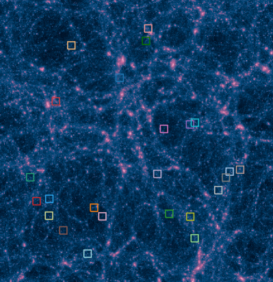
Figure 1.— Projected dark matter density at $z$ = 0 of the parent simulation, from which the 70 Caterpillar halos were selected. The box width is 100 $h^{-1}$ Mpc and the color represents the logarithm of the dark matter density. The colored circles correspond to the location of the first 24 $Caterpillar$ halos. The color for a given halo is kept identical for all figures throughout this work.

2.3. Contamination Study

As has been highlighted by Onorbe et al. (2014), a great deal of care has to be taken when carrying out re-simulations of this kind so as to avoid contamination of the main halo of interest by low-resolution particles at $z$ = 0. If mass from low resolution particles contributes more than $\sim$$2\%$ of the total host mass there can be offsets to estimates of the halo profile, shape, spin, and especially gas properties in hydrodynamic runs. To avoid contamination in our sample we custom built a Python GUI (using TraitsUI), Caterpillar Made Easy (cme), for running and analyzing cosmological simulations (for both single and multi-mass simulations). This tool allowed us to carry out an extensive contamination study (i.e., using $\sim$264 low resolution test halos with a particle mass of $\sim 10^{7}$ $\mathrm{M_{\sun}}$) specifically for the halos to be re-simulated. We have $automated$ the monotony of constructing hundreds of qualitatively similar $but$ quantitatively distinct cosmological simulations with the added benefit of being able to interactively select over initial condition parameters, cosmologies, halo finders and merger trees. This procedure was carried out self-consistently across all runs allowing for a systematic study of which simulation parameters produce the most computationally inexpensive to run, uncontaminated halos.

Using cme we tested eleven Lagrangian geometries (e.g., convex hull, ellipsoid, expanded ellipsoids, cuboids and expanded cuboids) so as to ensure a sphere of radius $\sim$1 $h^{-1}$ Mpc exists of purely uncontaminated (high-resolution) particles centered on the host halo at $z=0$. Our need to run eleven different Lagrangian geometries for each halo is motivated by the fact that the geometries vary substantially from halo to halo (due partially to their varied merger histories) and we wished to minimize the computation cost whilst achieving our contamination goals. It must also be highlighted that unlike many other studies, we did not select one Lagrangian geometry for all halos but used a specific geometry for a given halo depending on the needs of its simulation.

In Table 1 we show the various geometries we used for constructing our initial conditions. We modified music to be able to produce expanded Lagrangian volumes rather than the bounded volumes with which it was originally published. In Figure 2 we show four examples of Lagrangian geometries for halos selected for re-simulation. In some cases the geometries are reasonably compact allowing for the traditional minimum cuboid enclosing to be used. Some larger regions however are extremely non-spherical (e.g., bottom right of Fig. 2) and so a minimum ellipsoid was used. For each geometry we take the enclosed volume at $z$ = 0 denoted by either $4\times R_{{\rm vir}}(z=0)$ and $5\times R_{{\rm vir}}(z=0)$. We run each of these halos to $z$ = 0, run our modified rockstar and determine at what distance the closest low resolution or contamination particle (type = 2) resides in each case. With the knowledge that the high-resolution volume distance decreases at higher levels of refinement (Onorbe et al., 2014), we ensure a minimum contamination distance of $\sim$1 $h^{-1}$ Mpc at $z$ = 0 at our lowest resolution re-simulation with the desire to have uncontaminated spheres of radius, $\sim$1 Mpc at our highest resolution re-simulation. In cases where four times the virial radius enclosure created contaminated halos but five times the virial radius created too large a simulation to run, we opted for an expanded ellipsoid of the minimum enclosing ellipsoid. In some cases there were a handful of offending particles far away from the primary Lagrangian volume (e.g.,  Figure 2 top right and bottom left) making no standard geometry enclosure feasible, expanded or otherwise. Here we trimmed the Lagrangian volume by hand and simulated the new geometry to $z$ = 0 to ensure it had no contamination. Traditionally these types of halos are avoided but since we do not want to bias our sample, we dealt with complicated geometries in this specialized manner and have included them in our sample. Using this tailored approach, our highest resolution runs obtain very large, high-resolution regions with spheres of radius $\sim$$1.4\pm 0.4$ Mpc of solely high-resolution particles.

In Figure 3 we show box plots of the median contamination distance and respective quartiles for all 264 of our test halos using each of our selected geometries. Typically, the best performing geometry (i.e., the largest uncontaminated volume with the cheapest computational expense) was the expanded ellipsoid which enclosed all particles within 4 or 5 times the virial radius of the host in the parent simulation at $z=0$.

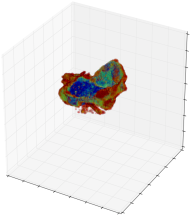
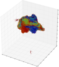
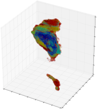
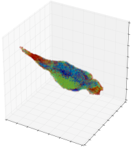
Figure 2.— Sample Lagrangian volumes (at $z$ = 127) of halos from the parent simulation. Some geometries are easily bounded by a minimum cuboid (e.g., top left) but others require an ellipsoid (e.g., bottom right). In some cases, there reside particles well away from the primary Lagrangian volume (e.g., top right and bottom left). For these difficult situations, we carefully trimmed the Lagrangian geometry to ensure no contamination of low resolution particles within 1 $h^{-1}$ Mpc of the host at $z$ = 0. Particles are color coded by distance from the host at $z$ = 0 where red particles are 5$\times$$R_{\mathrm{vir}}$ and blue particles are within the virial radius.

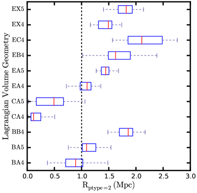
Figure 3.— Box plot of the distances to the first low resolution particle (particle type 2) for each of the prospective initial condition geometries (i.e., all run at levelmax = 11 in music, one level above our parent simulation). Table 1 contains the key for each geometry. The red lines indicate the median, edges of the box represent 25$\%$ and 75$\%$ quartiles and the outer tick marks represent the maximum and minimum distance. The dashed line represents the threshold we used to determine if a geometry was viable for a higher level re-simulation, though this was balanced against computational cost. We select the geometry which used the fewest CPU hours but maintained the largest uncontaminated volume.

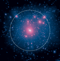
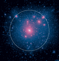
Figure 4.— Projected dark matter density at $z$ = 0 of Cat-1 at successively higher resolutions (increasing by a factor of 8 in mass resolution each time) from left to right. The left panel is lx = 11 ($m_{p}=1.53\times 10^{8}M_{\odot}$) and the right most panel is lx = 14 ($m_{p}=2.99\times 10^{4}M_{\odot}$). The white circle represents the virial radius, $R_{\mathrm{vir}}$. The image brightness is proportional to the logarithm of the dark matter density squared (i.e., log($\rho^{2}$).

Table 1The contamination suite used on the first refinement level (i.e., levelmax = 11) for every halo in the $Caterpillar$ suite.

Name	$nR_{vir}(z=0)^{a}$	Geometry	Factorb
CA4	4	Convex Hull	–
CA5	5	Convex Hull	–
EA4	4	Bounded Ellipsoid	–
EA5	5	Bounded Ellipsoid	–
EX4	4	Expanded Ellipsoid	1.05
EX5	5	Expanded Ellipsoid	1.05
EB4	4	Expanded Ellipsoid	1.1
EC4	4	Expanded Ellipsoid	1.2
BA4	4	Minimum Cuboid	–
BA5	5	Minimum Cuboid	–
BB4	4	Expanded Cuboid	1.1

2.4. Zoom-in Simulations

Starting from our parent simulation resolution, we re-simulated each halo at iteratively higher resolutions (a factor of 8x increase in particle number for each level) to ensure we did not obtain contaminated particles within the host halo (the uncontaminated volume shrinks with an increase in the ratio of the zoom-in resolution to that of the parent simulation resolution). In Figure 4, we show the dark matter distributions for iteratively higher resolutions of the same halo. One can clearly identify the same subhalos across all resolutions indicating the qualitative success of our numerical techniques. Regarding computational resources, each halo at our highest resolution took between 150 – 300K hours on TACC/Stampede and occupy $\sim$5 – 10 TB of storage for both the raw hdf5 snapshots and halo catalogue. Table 2 shows the mass and spatial resolution for each of our refinement levels. Our softening length is $\epsilon\sim$ 76 $h^{-1}$ pc for our fiducial resolution.

Table 2The resolution levels of the Caterpillar suite.

lx	$N_{p}$	$m_{p}$	$\epsilon$
		($\mathrm{M_{\sun}}$)	($h^{-1}$ pc)
15	327683	$3.7317\times 10^{3}$	38
14	163843	$2.9854\times 10^{4}$	76
13	80963	$2.3883\times 10^{5}$	152
12	40963	$1.9106\times 10^{6}$	228
11	20483	$1.5285\times 10^{7}$	452
10	10243	$1.2228\times 10^{8}$	904

Note. — lx represents represents the effective resolution ($N_{p}=(2^{X})^{3}$) of the high resolution region given by parameter, levelmax in music. $m_{p}$ is the particle mass and $\epsilon$ is the Plummer equivalent gravitational softening length. The parent simulation parameters are also shown in the last row. Only a select sample of halos are run at resolution level lx15. These runs will be presented in future works.

We space our snapshots (320 per simulation) in the logarithm of the expansion factor until $z$ = 6 ($\sim$5 Myrs/snapshot) and then linear in expansion factor down to $z$ = 0 ($\sim$50 Myrs/snapshot). The motivation for this piecewise stitching of the two temporal schemes is two-fold. At $z$ $>$ 6, we enter the era of mini-halo formation and the reionization epoch. If we wish to model the transport of Lyman-Werner (LW) radiation semi-analytically from the first mini-halos (e.g., Agarwal et al. 2012), we require a temporal resolution on par with the mean free path of LW photons in the intergalactic medium and the lifetime of a massive Population III star ($\leq$ 10 Myrs). Secondly, we also wish to resolve the disruption of low mass dwarf galaxies at low redshift, which requires a temporal resolution of order $\sim$ 50 Myrs (e.g., Segue I has a disruption time scale of $\sim$ 50 Myrs). These time scales are also required if one is attempting to determine subhalo orbital pericenters which can be input into semi-analytic models of tidal disruption (e.g., Baumgardt & Makino 2003). While we intend to use the capabilities offered by finely sampled snapshots in future work, this initial paper primarily focuses on the $z$ = 0 halo properties.

2.5. Iterative Unbinding In rockstar

rockstar is able to find any overdensity in 6D phase space including both halos and streams. To distinguish gravitationally bound halos from other phase space structures, rockstar performs a single-pass energy calculation to determine which particles are gravitationally bound to the halo. Over-densities where at least 50$\%$ of the mass is gravitationally bound are considered halos, with the exact fraction a tuneable parameter (unbound_threshold) of the algorithm (Behroozi et al., 2013).

This definition is generally very effective at identifying halos and subhalos – but it fails in two important situations. First, if a subhalo is experiencing significant tidal stripping, the 50$\%$ cutoff can remove a subhalo from the catalog that should actually exist. We have found that changing the cutoff can recover the missing subhalos, but the best value of the cutoff is not easily determined. Second, rockstar is occasionally too effective at finding substructure in our high resolution simulations. In particular, it often finds velocity substructures in the cores of our halos that are clearly spurious based on their mass accretion histories and density profiles. Importantly, these two issues do not just affect low mass subhalos, but they can also add or remove halos with $V_{\mathrm{max}}$ $>25$ km s^-1.

Both of these problems can be alleviated by applying an iterative unbinding procedure. We have implemented such an iterative unbinding procedure within rockstar. At each iteration, we remove particles whose kinetic energy exceeds the potential energy from other particles in that iteration. The potential is computed with the rockstar Barnes-Hut method (see Appendix B of Behroozi et al. 2013). We iterate the unbinding until we obtain a self-bound set of particles. Halos are only considered resolved if they contain at least 20 self-bound particles. All halo properties are then computed as usual, but with the self-bound particles instead of the one-pass bound particles. The iterative unbinding recovers the missing subhalos and removes most but not all of the spurious subhalos. Across 13 of our $Caterpillar$ halos, we recover 52 halos with subhalo masses above 10⁸ $\mathrm{M_{\sun}}$ which would have otherwise been lost using the conventional rockstar. Figure 5 demonstrates how these large haloes can be recovered when our iterative unbinding procedure is used.

To remove the remaining spurious subhalos, we also remove halos if $R_{\mathrm{max}}$ (i.e., the radius at which the velocity profile reaches its maximum) of the subhalo is larger than the distance between the subhalo and host halo centers. The downside to adding iterative unbinding is that it increases the run time for rockstar by $\sim$50$\%$. In the rest of this paper, we only consider subhalos with at least 20 self-bound particles passing the $R_{\mathrm{max}}$ cut. We define the subhalo mass, $M_{\mathrm{sub}}$, as the total gravitational bound mass of a subhalo which is obtained after the complete iterative unbinding procedure has been carried out.

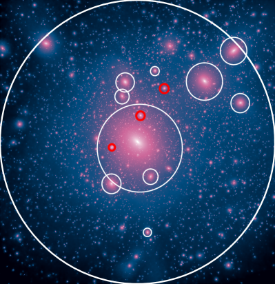
Figure 5.— Density projection of the Cat-1 halo with subhalos with $V_{\mathrm{max}}$ $>$ 30 km s^-1 highlighted by circles. The size of the circles corresponds to 3$\times$$R_{\mathrm{max}}$ (i.e., the radius at which the velocity profile reaches its maximum). The white circles indicate subhalos found by the default parameters of the halo finding algorithm rockstar (i.e., without iterative unbinding). The three red circles indicate halos which are recovered when complete iterative unbinding is used. The largest outer white circle indicates the virial radius of the host halo.

3. Results

3.1. Host Halo Properties

In Table 3, we provide the basic properties of our first 24 re-simulated halos. This includes the simulation name, the halo virial mass, the halo virial radius, concentration, maximum circular velocity, the radius at which the maximum circular velocity occurs, the formation time (defined as when the halo reaches half its present day mass), the redshift of the last major merger (1:3 mass ratio), the fraction of the host mass contained within subhalos, the axis ratios defining the halo shape, and the distance to the closest contamination particle from the host. We adopt a simple naming convention based on when the halos were post processed (1 – ${\rm N_{halos}}$). Where required, we use a shorthand reference to the resolution of the simulation. These refer to the parameter levelmax inside the IC generation code music (e.g., levelmax = 14 is simply lx14). This means lx14 represents an effective resolution of $N_{p}=(2^{14})^{3}$ ($\sim Aquarius$ level-2), lx13 $\rightarrow$ $N_{p}=(2^{13})^{3}$ ($\sim Aquarius$ level-3 or $\sim$$ELVIS$ resolution), lx12 $\rightarrow$ $N_{p}=(2^{12})^{3}$ and lx11 $\rightarrow$ $N_{p}=(2^{11})^{3}$. Unless otherwise stated, all halos in the analysis of this paper are the lx14 halos (i.e., our flagship resolution). All halos have similar $z$ = 0 properties except Cat-7 whose properties can be tied to the fact that it has recently undergone a massive merger (1:3 mass ratio at $z$ = 0.03). We obtain extremely large uncontaminated volumes ($\sim$1.4 Mpc) in all but one of our halos (Cat-18 is $\sim$$3\%$ contaminated by mass). The fraction of mass held in subhalos across our sample is $f_{m,subs}=0.121\pm 0.041$ (1$\sigma$), though this excludes Cat-7.

Table 3The halo properties of the first 24 $Caterpillar$ halos.

Halo	$M_{\mathrm{vir}}$	$R_{\mathrm{vir}}$	c	$V_{\mathrm{max}}$	$R_{\mathrm{max}}$	$z_{form}$	$z_{lmm}$	$f_{\mathrm{m,subs}}$	$c/a$	$b/a$	$R_{\mathrm{hires}}$
Name	($\times 10^{12}$ $\mathrm{M_{\sun}}$)	(kpc)		(km s-1)	(kpc)						(Mpc)
Cat-1	1.559	306.378	7.492	169.756	34.083	0.894	2.157	0.207	0.841	0.869	0.998
Cat-2	1.791	320.907	8.374	178.851	55.268	0.742	0.731	0.148	0.636	0.719	1.463
Cat-3	1.354	292.300	10.170	172.440	31.701	0.802	0.802	0.136	0.865	0.927	1.894
Cat-4	1.424	297.295	8.573	164.344	53.466	0.936	0.922	0.175	0.671	0.739	1.531
Cat-5	1.309	289.079	12.108	176.399	32.103	0.564	0.510	0.069	0.552	0.815	1.608
Cat-6	1.363	292.946	10.196	171.647	33.632	1.161	1.295	0.153	0.508	0.528	1.295
Cat-7	1.092	272.099	1.757	134.148	157.438	0.070	0.032	0.735	0.151	0.207	1.477
Cat-8	1.702	315.466	13.507	198.564	40.819	1.516	2.235	0.078	0.605	0.787	1.540
Cat-9	1.322	289.987	12.401	177.414	30.336	1.255	1.236	0.094	0.513	0.762	2.080
Cat-10	1.323	290.119	11.714	174.989	39.721	1.644	2.010	0.103	0.559	0.703	1.775
Cat-11	1.179	279.187	12.522	172.723	53.187	1.059	4.368	0.215	0.597	0.867	1.135
Cat-12	1.763	319.209	11.402	191.259	52.717	1.336	9.616	0.073	0.584	0.645	1.162
Cat-13	1.164	277.938	12.850	171.222	33.757	1.161	11.092	0.090	0.578	0.645	1.566
Cat-14	0.750	240.119	9.135	137.437	26.660	1.144	4.258	0.113	0.705	0.859	2.178
Cat-15	1.505	302.787	8.983	174.124	37.043	1.144	3.165	0.126	0.849	0.877	1.119
Cat-16	0.982	262.608	11.737	155.362	28.768	1.315	3.165	0.106	0.618	0.792	0.671
Cat-17	1.319	289.800	12.765	179.056	38.329	1.846	1.976	0.093	0.664	0.881	1.299
Cat-18	1.407	296.099	7.887	163.920	57.217	0.493	0.435	0.159	0.676	0.816	0.397
Cat-19	1.174	278.770	10.468	164.726	29.112	1.541	2.118	0.169	0.664	0.937	1.712
Cat-20	0.763	241.484	13.324	149.672	30.417	1.492	5.427	0.099	0.601	0.733	1.311
Cat-21	1.881	326.206	10.618	190.683	50.954	1.126	1.198	0.118	0.482	0.611	1.453
Cat-22	1.495	302.116	10.666	180.647	35.860	0.841	29.488	0.080	0.512	0.694	1.744
Cat-23	1.607	309.524	12.489	190.705	32.421	1.161	9.616	0.094	0.607	0.784	1.207
Cat-24	1.334	290.866	11.378	176.911	36.800	1.144	3.608	0.090	0.689	0.734	1.102
Mean*	1.368	291.791	10.903	173.167	38.886	1.144	4.410	0.121	0.634	0.771	1.402
$\pm$1$\sigma$	0.285	21.610	1.761	13.441	9.530	0.329	6.112	0.041	0.103	0.102	0.409

In Figure 6 we plot the concentration-mass (c-M) relation of the parent simulation for similarly sized halos (${\rm 11.5<log_{10}\ M_{\odot}<12.5}$, grey band indicating the 1$\sigma$ dispersion) and overlay the concentration ($R_{\mathrm{vir}}$/$R_{\mathrm{s}}$) and host mass of the high resolution halos. This shows that for nearly all of the halos, we are sampling within 68$\%$ of the average c-M relation at a fix halo mass. Again, Cat-7 is an outlier with an extremely low concentration because it recently underwent a major merger and has an extremely large substructure mass fraction so its concentration is not meaningful. For this reason we do not include it in the quantitative analysis in terms of determining average halo profile shapes or the mass function slopes. Its properties are still shown and plotted in the various tables and figures, however. Recently, Buck et al. (2015) found that the thickness of planes of satellites depends on the concentration of the host halo. Specifically, they found the thinnest planes are only found in the most concentrated, and hence earliest formed halos. The fact that we sample relatively average concentrations for halos of this mass range means that it is less likely that these hosts will contain planes of satellites, or if they do, their thicknesses will be quite large (Ji et al., in prep.). As the $Caterpillar$ sample grows, we will eventually sample overly concentrated halos, enabling us to see in better detail how this concentration-plane relation holds.

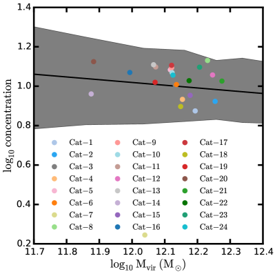
Figure 6.— Concentration-mass relation for the 24 $Caterpillar$ halos relative to those found in the parent simulation of similar mass. The concentration is defined as $r_{vir}/r_{s}$. Solid circles are the zoom-in simulations and the black line represents the concentration-mass relation drawn from the parent simulation for relaxed halos. The grey band is the 1$\sigma$ dispersion in the c–M relation for halos in the parent simulation between ${\rm 11.5<log_{10}\ M_{\odot}<12.5}$.

3.2. Visualizing The Halos $\&$ Their Assembly Histories

In Figures 7 and 8 we show images of the dark matter distribution in each of our 24 high-resolution halos at redshift $z=0$. The brightness of each pixel is proportional to the logarithm of the dark matter density squared (i.e. log($\rho^{2}$)projected along the line of sight. To enhance the density contrast, each panel has a different maximum density. We note that similarly colored pixel in one panel does not necessarily mean the density is the same for another panel. The panel width is 1 Mpc and the local dark matter density of the particles in each pixel is estimated with an SPH kernel interpolation scheme based on the 64 nearest neighbor particles. Upon first inspection it is clear that each halo is littered with an abundance of dark matter substructures of varied shapes and sizes. In some cases, there are reasonably large neighbors (e.g., Cat–4, 7, 11, 24). By virtue of our selection criteria these neighbors are no larger than 0.5$\times$$M_{\mathrm{vir}}$ of the central host. In any case, in under a Gyr, these SMC/LMC sized systems (M${}_{peak}>10^{11}$ $\mathrm{M_{\sun}}$) will likely undergo a major merger with the host galaxy.

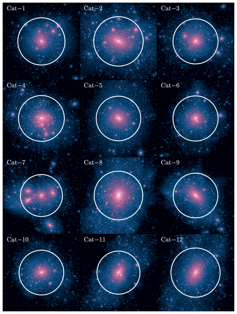
Figure 7.— Projected dark matter density at $z$ = 0 of the first 12 $Caterpillar$ halos with a box width of 1 Mpc. The image brightness is proportional to the logarithm of the dark matter density squared. Higher resolution images and animations are available at www.caterpillarproject.org.

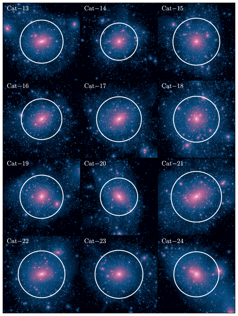
Figure 8.— Projected dark matter density at $z$ = 0 of each of the second set of 12 $Caterpilar$ halos with a box width of 1 Mpc. The image brightness is proportional to the logarithm of the dark matter density squared. Higher resolution images and animations are available at www.caterpillarproject.org.

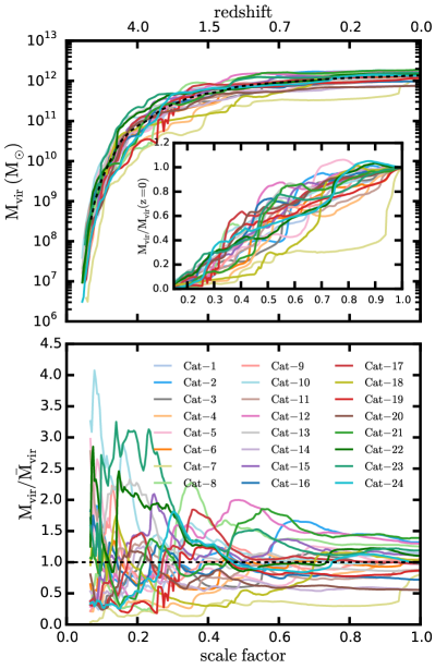
Figure 9.— Mass evolution of the first 24 Caterpillar halos. The top panel shows each halo evolution along with the mean (black dashed) evolution for each of the halos. The inset panel shows the mass evolution normalized to the halo mass at $z=0$. In the lower panel we show the mass evolution divided by the mean evolution to enhance individual features for each halo. We sample a diverse assembly history, from extremely quiet through to extremely violent (redshift of last major merger, $z$ $\sim$ 0.07).

In Figure 9 we show the mass evolution of each of the halos. As highlighted by the inset which shows the normalized mass evolution, there is a wide variety of formation histories. In our initial catalogue of 24 halos, six halos (Cat–2, 3, 4, 5, 7, 18) have had major mergers since $z=1$. The halos going above a normalized mass ratio of 1.0 have had a halo pass through them relatively recently which momentarily gives them extra mass such that it is larger than their $z$ = 0 mass (e.g, Cat–2). This indicates that many of the halos are yet to reach an equilibrium state.

Adopting the same criteria as Neto et al. (2007) we assess whether the host halos are relaxed. If their substructure mass fraction is below 0.1, their normalized offset between the center of mass of the halo (i.e., computed using all particles within $R_{\mathrm{vir}}$) and the potential center ($\mathrm{x_{off}\equiv|r_{c}-r_{cm}|/R_{vir}}$, ${\rm r_{c}\ \equiv}$ center of the potential well, ${\rm r_{cm}\ \equiv}$ center of mass) is below 0.07 and their virial ratio ($2T/|U|$) is below 1.35, then the host is considered relaxed. In Table 4 we provide the relaxed state of the halo. Many of the halos are in fact unrelaxed under this definition which is by design – we are sampling a wide range of assembly histories and so halos with recent merger events that prevent the halos from being fully virialized naturally make up part of our sample.

3.3. Host Halo Profiles

In Figure 10 we plot the spherically averaged halo profiles for each of our 24 simulated halos. We draw the measured density profile as a thick line of a given color and continue the fit beyond the smallest radius possible set by Power et al. (2003) as a vertical black dashed line. We truncate each fit at this radius. There is a clear diversity in the profile shapes owing in part to the assembly histories of each halo. Halos which have undergone a recent major merger whose substructure mass fractions are higher than average are primarily dominated by a single subhalo (e.g, Cat–7 has a large subhalo at 200 kpc). The fitting formula we have used to describe the mass profile of our simulated halos follow the method of Navarro et al. (2010) and is given by the following Einasto form (over all particles within the virial radius):

$${\rm log[\rho(r)/\rho_{-2}]=(-2/\alpha)\left[(r/r_{-2})^{\alpha}-1\right]}.$$ (1)

The $r_{-2}$ is the scale length of the halo which can be obtained without resorting to a particular fitting formula. We compute the logarithm of the slope profile and identify where a low-order polynomial fit to it intersects the isothermal value ($\gamma=2$). Unlike the Navarro-Frenk-White profile (NFW) the peak parameter in the Einasto profile, $\alpha$, is allowed to vary and thus provides a third parameter for the fitting formula. The best fitting parameters are found by minimizing the deviation between model and simulation at each bin. Specifically we minimize the function $Q^{2}$, defined as:

$${\rm Q^{2}=\frac{1}{N_{bins}}\sum\limits_{i=1}^{N_{bins}}(ln(\rho_{i})-ln(\rho^{model}_{i}))^{2}.}$$ (2)

In this manner we find a function which clearly illustrates the deviation of the simulated and model profiles. In Table 4 we show our minimum $Q^{2}$ parameter ($Q_{min}$), characteristic scale radius $r_{-2}$, and their corresponding densities for each halo. For our relaxed halos, $Q_{min}$ for our Einasto fits are 0.027 $\pm$ 0.010 indicating reasonable agreement between the simulated and model Einasto profiles. This is better than our NFW profile fits for which we obtain $Q_{min}=0.055\pm 0.020$. The peak parameters for our Einasto fits are 0.169 $\pm$ 0.023 which is comparable to those of the $Aquarius$ halos ($\alpha$ = 0.145 – 0.173) studied in Navarro et al. (2010). For halos which significantly deviate from the mean, it is important to note that those halos are not relaxed and so by definition will not provide meaningful Einasto/NFW fits. A more detailed study of the halo density profiles are reserved for future work.

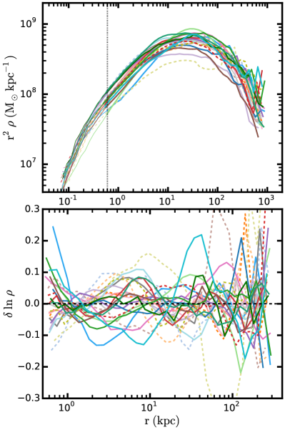
Figure 10.— Upper panel: Normalized halo profiles for each of the host halos. Relaxed (solid lines) halos are better fit by Einasto profiles ($\alpha\sim 0.16$) over NFW profiles though for halos that are unrelaxed (dashed lines), they are unable to be properly fit by NFW or Einasto profiles which is in agreement with Neto et al. (2007) and Navarro et al. (2010). This inability stems purely from their definition, which a priori assumes that the halos are in virial equilibrium which is clearly not the case for halos which have undergone a recent merger. The dashed black line indicates the Power et al. (2003) resolution limit as set by our softening length (also represented by a thinner density profile line). Lower panel: The log of the ratio between each of the Einasto fits and the data between the Power et al. (2003) radius and the virial radius.

Table 4The relaxed nature and Einasto profile parameters for the first 24 $Caterpillar$ halos. For comparison, $Q_{min}$ fits for NFW halo profiles are also listed.

Halo	Relaxed	$\rho_{-2}$	$r_{-2}$	$\alpha$	$Q_{min}$	$Q_{min}$
Name			($\times 10^{5}$)		Ein.	NFW
Cat-1	✗	9.929	27.182	0.128	0.039	0.103
Cat-2	✓	3.531	46.846	0.185	0.040	0.033
Cat-3	✓	11.604	25.309	0.151	0.028	0.067
Cat-4	✗	5.504	34.962	0.154	0.039	0.080
Cat-5	✓	13.305	24.152	0.167	0.018	0.050
Cat-6	✗	9.254	28.299	0.164	0.027	0.058
Cat-7	✗	0.482	90.528	0.075	0.082	0.162
Cat-8	✓	8.027	34.555	0.236	0.033	0.036
Cat-9	✓	12.159	25.543	0.186	0.011	0.034
Cat-10	✓	14.482	23.492	0.168	0.029	0.049
Cat-11	✗	10.617	25.450	0.173	0.049	0.071
Cat-12	✓	8.897	31.157	0.160	0.030	0.062
Cat-13	✓	11.842	25.010	0.187	0.009	0.036
Cat-14	✓	10.455	21.347	0.139	0.018	0.078
Cat-15	✓	8.905	28.744	0.139	0.025	0.078
Cat-16	✓	10.445	24.162	0.166	0.026	0.056
Cat-17	✓	11.283	26.799	0.195	0.019	0.026
Cat-18	✗	6.998	31.012	0.150	0.023	0.082
Cat-19	✗	9.079	26.881	0.164	0.032	0.054
Cat-20	✓	11.415	22.158	0.199	0.018	0.020
Cat-21	✓	6.682	36.486	0.175	0.025	0.043
Cat-22	✓	10.857	26.957	0.156	0.017	0.063
Cat-23	✓	13.486	26.024	0.172	0.018	0.039
Cat-24	✓	7.040	31.734	0.181	0.044	0.050
Mean*	-	9.817	28.446	0.169	0.027	0.055
$\pm$1$\sigma$	-	2.6106	5.5677	0.023	0.010	0.020

3.4. Subhalo Properties

In Figure 11a we show the cumulative abundance of subhalos as a function of their maximum circular velocity for each $Caterpillar$ halo. Since we achieve excellent convergence (see Appendix A), we reliably resolve halos with circular velocities of $\sim$4 km s^-1, which is crucial for identifying the sites of first star formation. At the high $V_{\mathrm{max}}$ end we find a variety of different sized subhalos for each host. Some hosts have only one 10 km s^-1 subhalo whereas another host halo has a large 70 km s^-1 subhalo within the virial radius. Between 5-20 km s^-1 all halos are very similar in their $V_{\mathrm{max}}$ function slopes within a slight offset owing to normalization stemming from the differences in host halo mass. At low $V_{\mathrm{max}}$ values ($\sim$$3$ km s^-1) we begin to lose completeness of our host subhalo sample due to lack of resolution. We additionally include in this Figure the $V_{\mathrm{max}}$ function for subhalos at infall (i.e., when a subhalo first crosses the virial radius of the host). Since dynamical friction affects the highest mass subhalos the fastest, the biggest difference in the functions occurs at the high-mass end whereby several LMC sized systems ($M_{\mathrm{peak}}$ $>$ $10^{11}\ M_{\odot}$) have been destroyed (over a time scale of 1 – 2 Gyrs) between infall and $z$ = 0. These large LMC sized-systems at infall can host anywhere from 4 – 30$\%$ of the Milky Way sized halo’s subhalos at $z=0$ depending on their orbit and infall time (Griffen et al. in prep.). In solid black we also plot the $Aquarius$ Aq-A2 halo from Springel et al. (2008) (using the same version of rockstar that we used for the $Caterpillar$ halos). We find the differences in the cosmology ($\sigma_{8}=0.9$) and the slightly higher resolution of $Aquarius$ leads to systematic differences in subhalo abundance.

In Figure 11b, we show the subhalo mass functions for each of the halos. Our results are best fit by the power law d$N$/d$M\propto M^{-1.88\pm 0.10}$, which is less steep than that found in the $Aquarius$ halos of Springel et al. (2008). This slope is the best fit over the ranges $10^{5}\--10^{8}$ $\mathrm{M_{\sun}}$. We do observe a scatter in the subhalo abundances. This can be explained by the subtle concentration-subhalo-abundance relation whereby for fixed halo mass, there are more (less) subhalos belonging to hosts which are less (more) concentrated (e.g, Zentner et al. 2005, Watson et al. 2011, Mao et al. 2015). Indeed, we find halos which are more concentrated (see Figure 6) have lower normalizations than those less concentrated at fixed $V_{\mathrm{max}}$. This is simply because halos which are more concentrated have formed earlier and so subhalos have spent substantially longer undergoing dynamical disruption within the host compared to similar sized subhalos orbiting less concentrated hosts.

In Figure 11c we show the subhalo radial mass fraction which indicates high variability in the contribution to the total halo mass from substructure as a function of galactocentric distance. For example, at 0.1$R_{\mathrm{vir}}$, the total mass contributing to the host halo mass from substructure varies by a factor of 10 or more when normalized by mass. At $R_{\mathrm{vir}}$ our substructure mass fraction varies by $\sim 10\%$ (see Table 3 for exact fractions). Cat-7 has a large component of the halo mass in substructure at low radii because it has recently undergone a major merger (z = 0.03). Those halos with a large substructure mass fraction generally have had a recent major merger and are in the process of disrupting the recently accreted systems. On average, for a fixed fraction of the virial radius, the $Caterpillar$ halos have less mass in substructure than that found in the Aq-A $Aquarius$ halo (see solid black line, calculated using the exact same code). In Figure 11d we plot the normalized number of subhalos as a function of radius scaled by the virial radius of the host. We find the scatter in the number of subhalos as a function of galactocentric distance is a factor of 3 across all halos except within the inner 10$\%$ of the host halo where we are subject to noise in the halo finding produced by rockstar. Again, in solid black we also plot the $Aquarius$ Aq-A2 halo from Springel et al. (2008). We find the differences in the cosmology ($\sigma_{8}=0.9$) and in particular the slightly higher resolution of $Aquarius$ leads to this systematic difference in the subhalo number density.

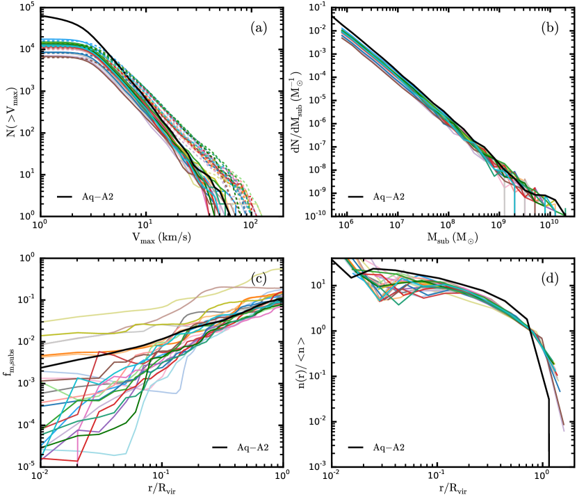
Figure 11.— (a) The cumulative abundance of subhalos as a function of their maximum circular velocity ($V_{\mathrm{max}}$) for each of the $Caterpillar$ halos. The solid lines represent subhalos at $z=0$ and the dashed lines represent halos at infall (i.e., when they first cross the virial radius of the host). Many of the SMC/LMC sized systems ($M_{\mathrm{peak}}$ $>10^{11}$ $\mathrm{M_{\sun}}$) are destroyed by $z$ = 0, though some large subhalos do survive. The $Caterpillar$ suite is complete down to $\sim$4 km s^-1. See our convergence study in the Appendix A. The solid black line is that of the Aquarius-A halo at a similar resolution (level-2, Springel et al. 2008). (b) The subhalo mass functions for each of the host halos. When normalized by mass, the range $10^{-6}\--10^{-4}$ $\mathrm{M_{\sun}}$ there is small scatter in the subhalo abundances as all of our hosts are very similar in mass. Over the ranges 10^6-8 $\mathrm{M_{\sun}}$ we obtain a median mass function slope of -1.88 $\pm$ 0.1, slightly shallower than Aquarius ($\alpha\sim 1.90$). As we move to higher and lower mass regimes, there are differing abundances of large and small subhalos for each host. There are a number of systems with $\sim 10^{9\--10}$ $\mathrm{M_{\sun}}$ halos within the virial radius of the host making them possible Large/Small Magellanic Cloud analogues. Again, the solid black line is that of the Aquarius-A. (c) The subhalo mass fraction as a function of radius scaled by the virial radius of the host. The substructure mass is distributed similarly in nearly all halos with the exception of Cat–7 which has undergone a major merger. There is more variability in the substructure mass fraction at low radii owing to the on-going disruption most prevalent in the inner most dense regions of each host. (d) The normalized number of subhalos as function of radius scaled by the virial radius of the host. The number of subhalos as a function of distance is extremely self-similar across all halos except within the inner 10$\%$ of the virial radius of each host. This is in agreement with the findings of Springel et al. (2008) when factoring in their slightly higher resolution of the $Aquarius$ suite and use of the observationally disfavoured high value of $\sigma_{8}$ ($\sigma_{8}$ = 0.9).

3.5. Too Big To Fail

We also examine halos which are massive enough to form stars but have no luminous counterpart in the nearby Universe (i.e., the too big to fail problem, hereafter TBTF, Boylan-Kolchin et al. 2011). To do this we select halos with $V_{\mathrm{peak}}$ $>$ 30 km s^-1 which are subhalos large enough to retain substantial gas in the presence of an ionizing background and therefore theoretically should form stars. We follow the same definition as in Garrison-Kimmel et al. (2014a) to count two classes of halos. Strong massive failures are too dense to host any of the currently known bright MW classical dwarf spherioidals (dSph) galaxies. Massive failures (MFs) include all strong massive failures (SMFs) as well as all massive subhalos which have densities consistent with the high-density dSphs (i.e., Draco and Ursa Minor) but can not be associated with them without allowing a single dwarf galaxy to be hosted by multiple halos (i.e., assuming every observable dSph galaxy is hosted by exactly one halo). Most subhalos in the range of $V_{\mathrm{max}}$ = 25 – 30 km s^-1 could host a low-density dwarf and as such are not defined as massive failures.

In Figure 12, we plot a sample of the rotation curves for three different $Caterpillar$ halos (Cat-19, Cat-13 and Cat-18). We adopt the Boylan-Kolchin et al. (2012) Einasto correction for $R<291$ pc, which differ from the $ELVIS$ profile fits in that they extrapolate their entire profile from $R_{\mathrm{max}}$ with various density profile shapes. Black squares depict circular velocities of the classical dwarf galaxies (with luminosities above $2\times 10^{5}$ L_⊙,V), as measured by Wolf et al. (2010). Dashed-dot cyan lines are LMC analogues (i.e., $V_{\mathrm{max}}$ $>$ 60 km s^-1 which are excluded from our failure analysis), blue dashed lines are massive failures and red solid lines are strong massive failures. Thin black solid lines are subhalos which pass the test of having at least one observed dwarf with a comparable circular velocity, i.e., a circular profile goes through one of the observed dwarf galaxy data points. The cumulative number of profiles above and below the observed classical dwarfs for Cat-19 are 10 MFs, 5 SMFs and one LMC analogue. Similarly we find Cat-13 has 11 MFs and 8 SMFs. Cat-18 has the most failures of any halo with 21 MFs and 14 SMFs with one LMC analogue.

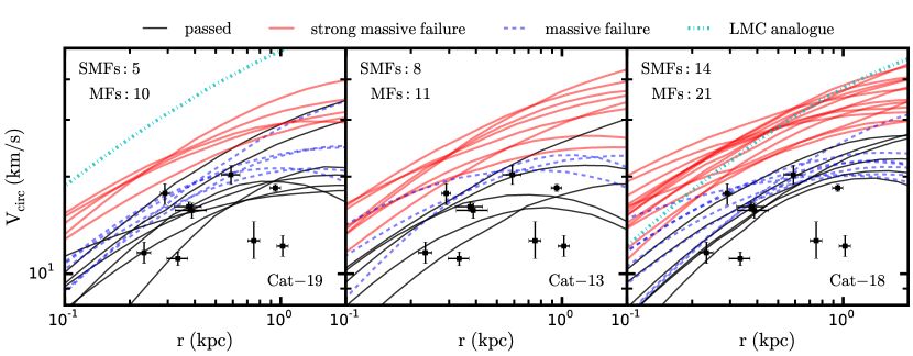
Figure 12.— The rotation curves for all subhalos identified with a peak maximum circular velocity $V_{\mathrm{peak}}$, above 30 km s^-1 within 300 kpc of three different $Caterpillar$ hosts. The black squares indicate observational constraints from dwarf galaxies from Wolf et al. (2010). We only include those observed systems whose luminosities are above $2\times 10^{5}$ L_⊙,V (i.e., showing only classical dwarfs and excluding ultra-faint dwarf galaxies). Dashed-dot cyan lines are LMC analogues (i.e., $V_{\mathrm{max}}$ $>$ 60 km s^-1), blue dashed lines are massive failures (MFs) and red solid lines are strong massive failures (SMFs). Thin black solid lines are subhalos pass the check and have at least one observed dwarf with a comparable circular velocity (i.e., one halo passes through the circular velocity of a known classical dwarf determined by Wolf et al. 2010).

In Figure 13 we plot the number of strong and massive failures across all Caterpillar halos. Specifically we plot the fraction of hosts with fewer than N MFs and N SMFs within 300 kpc of each host as a function of N (black lines). Averaging over the entire Caterpillar sample (excluding Cat-7 as it has recently had a massive major merger), we predict 8 $\pm$ 3 (1$\sigma$) SMFs and 16 $\pm$ 5 (1$\sigma$) MFs within 300 kpc. If the Milky Way were well described by such an average we would expect to have these failures.

For comparison, we plot the $ELVIS$ MF and SMF counts (red lines). The lower resolution in these simulations requires an extrapolation of the velocity profile from $V_{\mathrm{max}}$ and $R_{\mathrm{max}}$ using an analytic Einasto profile. Qualitatively, both simulation suites agree that there are a significant number of both MFs and SMFs. Quantitatively, there are several differences, which we now describe. The $Caterpillar$ suite has many more MFs. This is due to our ability to better resolve high $V_{\mathrm{peak}}$ subhalos that have been tidally stripped. In particular, the iterative unbinding procedure described in Section 2.5 removes the need for the rockstar unbound_threshold parameter (Behroozi et al., 2013). We can simulate the effect of the standard unbound_threshold = 0.5 cut by removing halos whose bound mass is less than 50$\%$ of their mass prior to unbinding. The MF counts with this cut are shown in Figure 13 by the blue lines, which are very similar to the $ELVIS$ MF counts.

The $Caterpillar$ suite also has significantly fewer SMFs compared to $ELVIS$. This discrepancy is likely due to the fact that we have measured rather than extrapolated the subhalo density profiles. Variations in the Einasto shape parameter ($\alpha$) greatly affect the massive failure count (see Figure 4 of Garrison-Kimmel et al. 2014a). The Einasto fits to our density profiles have $\alpha$ typically closer to 0.2, which is less discrepant.

Whilst TBTF is a prevalent problem in pure $N$-body simulations, many authors have indicated the tension between the circular velocities of observed classical dwarfs and simulated subhalos can be alleviated with the addition of supernovae feedback and ram pressure stripping (e.g., Pontzen & Governato 2012, Zolotov et al. 2012, Arraki et al. 2014, Brooks et al. 2013, Del Popolo et al. 2014, Gritschneder & Lin 2013, Elbert et al. 2015, Maxwell et al. 2015) or by making dark matter self-interacting (e.g., Vogelsberger et al. 2012, Zavala et al. 2013). Our results are within 1$\sigma$ of the number of failures found by Garrison-Kimmel et al. (2014a) (i.e., 12 massive failures within 300 kpc), even when using a better density profile estimation.

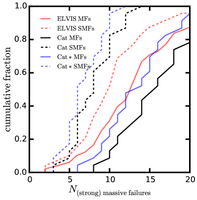
Figure 13.— Cumulative fraction of massive failures (MFs) and strong massive failures (SMFs) across all $Caterpillar$ halos (excluding Cat-7 which has undergone a recent massive major merger). We predict 8 $\pm$ 3 (1$\sigma$) strong massive failures and 16 $\pm$ 5 (1$\sigma$) massive failures within 300 kpc of the Milky Way. We also include the result from Garrison-Kimmel et al. (2014a) (i.e, using $\alpha=0.15$ Einasto profiles) as a reference. The black lines are all failures which are detected by our version of rockstar which includes iterative unbinding. The blue lines are all failures found using a cut which mimics rockstar without iterative unbinding (see Section 3.5 text for details). This indicates a fraction of failures are undergoing tidal disruption which may have been unaccounted for in the $ELVIS$ subhalo catalogues.

4. Conclusion

In this work we have presented the first results of the $Caterpillar$ simulation project, whose goal is to better understand the formation of Milky Way-sized galaxies and their satellite companions at both high and low redshift. We have carried out 24 initial simulations in a $Planck$ based $\Lambda$CDM cosmology. Although the total halo number will increase to 60 – 70 shortly, these first 24 halos provide us with an exquisite initial set of data to achieve our first set of science goals. In our approach, we have taken exceptional care to validate our numerical techniques. We quadruple the current number of halos available in the literature at this extremely high mass and temporal resolution, allowing for detailed statistical studies of the assembly of Milky Way-sized galaxies. We additionally have adjusted our simulation parameters to be more inclusive of potential scientific questions not yet studied in simulations of this size (i.e., decreasing the temporal resolution to $\sim$5 Myrs/snapshot and increasing the volume resolved by high-resolution particles to 1–2 Mpc). The results presented above demonstrate our data quality and give initial clues at how halo properties vary across large numbers of realizations. Our initial key results can be summarized as follows:

1. Key halo properties such as the halo profile, mass functions and substructure fractions are intimately connected to each halo’s overall assembly history. Halos which have undergone recent major mergers have profiles which are poorly fit by either the NFW or Einasto profile. For those halos which are well fit by Einasto profiles, they have peak $\alpha$ values of 0.169 $\pm$ 0.023. Excluding the Cat-7 halo, we find a $Q_{min}=0.027\pm 0.010$ indicating reasonable agreement with Einasto fits of the $Aquarius$ halos.

2. The abundance of dark matter subhalos remains relatively similar across our sample when normalized to host halo. As such, our halo mass functions are best fit by a simple power law, d$N$/d$M\propto M^{-1.88\pm 0.10}$. The scatter in the normalizations of the mass functions is due to the concentration-subhalo abundance relation for fixed halo mass (i.e., our more concentrated halos exhibit lower normalizations for fixed $\mathrm{M}_{host}$).

3. Regarding TBTF, dividing halos into two categories of massive failures and strong massive failures we predict 8 $\pm$ 3 (1$\sigma$) strong massive failures and 16 $\pm$ 5 (1$\sigma$) massive failures within 300 kpc of the Milky Way.

4. Iterative unbinding in rockstar must be included to properly recover all bound subhalos this resolution. We recover 52 halos above 10⁸ $\mathrm{M_{\sun}}$ across a sample of 13 $Caterpillar$ halos ($\sim$4 per host halo) using iterative unbinding which would have otherwise been unaccounted for using traditional rockstar. This means that a small fraction of massive subhalos undergoing heavy tidal disruption may be unaccounted for in studies using traditional rockstar (e.g., the $ELVIS$ halo catalogues).

This paper outlines the data products of the $Caterpillar$ simulations and sets the foundation of many upcoming in-depth studies of the Local Group. Through our statistical approach to the assembly of Milky Way-sized halos we will gain a more fundamental insight into the origin and formation of the Galaxy, its similar sized cousins and their respective satellites.

Appendix A: Convergence Study

In Figure 14 we plot the halo profiles (Cat-2) and maximum circular velocity functions (Cat-9) at all our resolutions. We find our halos are well converged down to $\sim$0.2$\%$ of $R_{\mathrm{vir}}$. In the case of the $V_{\mathrm{max}}$ functions, we find we are converged down to $\sim$4 km s^-1 at our highest resolution. When normalized to the host halo virial velocity, the halos are in excellent agreement with one another. Halos were re-simulated at successively higher and higher mass and spatial resolution from the initial parent volume. In each instance, care was taken to ensure all halo properties were numerically converged (provided that quantity was not resolution limited, e.g. halo shape). In Table 5 and 6 we show the same quantities as in Table 3 from the text but this time include the lower resolution halo properties. A full resolution study will be provided at the website, http://www.caterpillarproject.org when the LX15 runs have been completed.

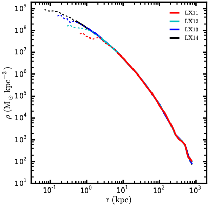
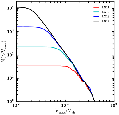
Figure 14.— Convergence test for the Cat-2 and Cat-9 halos illustrating convergent halo profiles and $V_{\mathrm{max}}$ functions respectively. Panel (a) normalized halo profiles where the thick line represents the density profile above the radius defined by Power et al. (2003). The thin dashed line of the same color is the profile extrapolated down to the softening length. Panel (b) the cumulative abundance of subhalos as a function of their maximum circular velocity ($V_{\mathrm{max}}$) . These halos are representative of the convergence we achieve for all $relaxed$ $Caterpillar$ halos.

Table 5Halo properties for the first set of 12 $Caterpillar$ halos at each resolution.

Name	Geometry	$n$$R_{\mathrm{vir}}$	lx	$M_{\mathrm{vir}}$	$R_{\mathrm{vir}}$	c	$V_{\mathrm{max}}$	$R_{\mathrm{max}}$	$z_{0.5}$	$z_{lmm}$	$f_{\mathrm{m,subs}}$	b/c	c/a	$R_{\mathrm{res}}$
				($10^{12}$ $\mathrm{M_{\sun}}$)	(kpc)		(km s-1)	(kpc)						(Mpc)
Cat-1	EA	5	11	1.579	307.690	7.762	172.293	35.049	0.881	2.118	0.161	0.810	0.828	1.391
			12	1.560	306.491	7.494	171.060	34.292	0.894	2.118	0.171	0.824	0.869	1.248
			13	1.560	306.458	7.647	170.707	36.451	0.894	2.157	0.197	0.842	0.883	1.138
			14	1.559	306.378	7.492	169.756	34.083	0.894	2.157	0.207	0.841	0.869	0.998
Cat-2	EB	4	11	1.807	321.876	7.621	176.924	64.931	0.742	0.719	0.092	0.596	0.724	1.577
			12	1.782	320.357	8.575	179.069	53.856	0.742	0.719	0.112	0.607	0.716	1.522
			13	1.792	320.970	8.382	178.753	54.360	0.742	0.731	0.137	0.643	0.731	1.480
			14	1.791	320.907	8.374	178.851	55.268	0.742	0.731	0.148	0.636	0.719	1.463
Cat-3	EB	4	11	1.343	291.538	10.763	175.066	26.554	0.802	0.790	0.079	0.961	0.971	1.966
			12	1.355	292.387	10.489	175.142	29.083	0.802	0.790	0.100	0.868	0.915	1.926
			13	1.355	292.400	10.523	172.946	31.565	0.802	0.802	0.117	0.850	0.905	1.906
			14	1.354	292.300	10.170	172.440	31.701	0.802	0.802	0.136	0.865	0.927	1.894
Cat-4	EB	4	11	1.503	302.676	8.308	169.309	91.132	0.894	0.908	0.128	0.749	0.825	1.791
			12	1.415	296.632	9.208	168.170	85.989	0.922	0.922	0.120	0.681	0.762	1.594
			13	1.434	298.009	8.434	164.999	59.225	0.936	0.922	0.156	0.673	0.743	1.561
			14	1.424	297.295	8.573	164.344	53.466	0.936	0.922	0.175	0.671	0.739	1.531
Cat-5	EB	4	11	1.306	288.846	11.897	173.913	33.844	0.584	0.519	0.025	0.551	0.835	1.676
			12	1.318	289.714	11.896	174.223	36.356	0.574	0.519	0.041	0.547	0.765	1.657
			13	1.314	289.450	12.324	176.818	29.346	0.574	0.519	0.055	0.556	0.825	1.617
			14	1.309	289.079	12.108	176.399	32.103	0.564	0.510	0.069	0.552	0.815	1.608
Cat-6	EB	4	11	1.371	293.516	10.373	172.100	32.944	1.144	1.275	0.094	0.495	0.534	1.708
			12	1.347	291.848	10.522	172.873	30.622	1.161	1.275	0.116	0.496	0.525	1.495
			13	1.366	293.186	10.086	170.858	32.794	1.161	1.295	0.138	0.510	0.529	1.300
			14	1.363	292.946	10.196	171.647	33.632	1.161	1.295	0.153	0.508	0.528	1.295
Cat-7	EB	4	11	1.142	276.168	2.513	139.055	140.859	0.065	0.057	0.693	0.191	0.301	1.756
			12	1.111	273.686	2.487	136.803	145.085	0.074	0.057	0.615	0.170	0.288	1.520
			13	1.091	272.009	1.674	133.574	162.291	0.065	0.036	0.693	0.168	0.235	1.510
			14	1.092	272.099	1.757	134.148	157.438	0.070	0.032	0.735	0.151	0.207	1.477
Cat-8	EB	4	11	1.729	317.150	13.081	198.577	46.800	1.541	2.195	0.032	0.602	0.768	1.690
			12	1.716	316.337	13.154	198.229	39.671	1.315	2.195	0.053	0.594	0.775	1.597
			13	1.701	315.450	13.340	197.637	39.810	1.516	2.235	0.066	0.599	0.791	1.550
			14	1.702	315.466	13.507	198.564	40.819	1.516	2.235	0.078	0.605	0.787	1.540
Cat-9	EB	4	11	1.330	290.616	12.568	177.522	32.309	1.236	1.217	0.050	0.493	0.762	2.383
			12	1.331	290.654	11.616	175.047	27.903	1.236	1.236	0.070	0.486	0.754	2.101
			13	1.329	290.538	12.132	176.808	30.297	1.255	1.236	0.085	0.500	0.754	1.833
			14	1.322	289.987	12.401	177.414	30.336	1.255	1.236	0.094	0.513	0.762	2.080
Cat-10	EB	4	11	1.319	289.809	11.902	175.553	41.894	1.699	2.010	0.052	0.561	0.709	1.983
			12	1.332	290.764	11.439	174.479	29.806	1.516	2.010	0.069	0.551	0.679	1.870
			13	1.328	290.477	11.714	175.124	25.839	1.644	2.010	0.088	0.559	0.703	1.740
			14	1.323	290.119	11.714	174.989	39.721	1.644	2.010	0.103	0.559	0.703	1.775
Cat-11	EB	4	11	1.194	280.361	10.551	165.980	62.881	1.059	4.368	0.175	0.527	0.719	1.490
			12	1.196	280.471	10.044	163.290	70.202	1.043	4.368	0.200	0.525	0.703	1.408
			13	1.190	280.043	12.272	173.893	45.727	1.059	1.644	0.199	0.590	0.868	1.192
			14	1.179	279.187	12.522	172.723	53.187	1.059	4.368	0.215	0.597	0.867	1.135
Cat-12	EA	5	11	1.786	320.627	11.723	191.564	59.256	1.336	2.542	0.034	0.592	0.724	1.664
			12	1.749	318.388	11.824	192.085	56.859	1.336	2.542	0.042	0.572	0.686	1.342
			13	1.767	319.441	11.663	191.320	49.435	1.336	2.542	0.062	0.571	0.703	1.239
			14	1.763	319.209	11.402	191.259	52.717	1.336	9.616	0.073	0.584	0.645	1.162

Notes: The resolution details for each refinement level (i.e. 11, 12, 13, 14) can be found in Table 2 and the geometry definitions in Table 1.

Table 6Halo properties for the second set of 12 $Caterpillar$ halos at each resolution.

Name	Geometry	$n$$R_{\mathrm{vir}}$	lx	$M_{\mathrm{vir}}$	$R_{\mathrm{vir}}$	c	$V_{\mathrm{max}}$	$R_{\mathrm{max}}$	$z_{0.5}$	$z_{lmm}$	$f_{\mathrm{m,subs}}$	b/c	c/a	$R_{\mathrm{res}}$
				($10^{12}$$\mathrm{M_{\sun}}$)	(kpc)		(km/s)	(kpc)						(Mpc)
Cat-13	EB	4	11	1.168	278.303	12.664	169.603	31.214	1.180	11.092	0.042	0.595	0.652	2.069
			12	1.171	278.509	12.979	170.750	31.408	1.161	14.748	0.063	0.575	0.634	1.742
			13	1.163	277.896	13.052	171.892	34.163	1.161	15.750	0.073	0.580	0.655	1.634
			14	1.164	277.938	12.850	171.222	33.757	1.161	11.092	0.090	0.578	0.645	1.566
Cat-14	EC	4	11	0.744	239.430	9.526	137.580	42.772	1.180	4.155	0.060	0.714	0.851	2.516
			12	0.757	240.865	8.854	136.512	27.875	1.144	4.258	0.086	0.709	0.849	2.301
			13	0.754	240.529	9.148	137.266	44.395	1.144	4.258	0.097	0.694	0.842	2.234
			14	0.750	240.119	9.135	137.437	26.660	1.144	4.258	0.113	0.705	0.859	2.178
Cat-15	EX	5	11	1.501	302.562	8.950	173.834	31.210	1.144	3.165	0.072	0.897	0.912	1.669
			12	1.497	302.281	9.223	174.792	33.832	1.144	3.165	0.089	0.897	0.926	1.630
			13	1.504	302.755	9.077	174.431	36.520	1.144	3.165	0.111	0.837	0.861	1.597
			14	1.505	302.787	8.983	174.124	37.043	1.144	3.165	0.126	0.849	0.877	1.119
Cat-16	EB	4	11	0.993	263.614	10.997	154.748	42.280	1.315	3.165	0.053	0.567	0.765	1.406
			12	0.976	262.082	12.099	156.589	28.820	1.315	3.165	0.072	0.593	0.791	1.393
			13	0.980	262.447	11.888	156.193	29.498	1.315	3.165	0.088	0.597	0.766	1.384
			14	0.982	262.608	11.737	155.362	28.768	1.315	3.165	0.106	0.618	0.792	0.671
Cat-17	EX	4	11	1.311	289.204	13.216	178.671	38.818	1.846	1.943	0.038	0.646	0.794	1.525
			12	1.314	289.456	12.906	178.676	39.713	1.846	1.943	0.057	0.680	0.875	1.427
			13	1.329	290.487	12.505	178.763	38.717	1.846	1.976	0.084	0.657	0.863	1.333
			14	1.319	289.800	12.765	179.056	38.329	1.846	1.976	0.093	0.664	0.881	1.299
Cat-18	EX	4	11	1.428	297.536	7.909	167.184	32.058	0.451	0.427	0.100	0.677	0.847	1.491
			12	1.414	296.559	7.861	164.702	48.041	0.459	0.412	0.123	0.720	0.840	1.397
			13	1.400	295.596	7.823	165.164	40.766	0.493	0.435	0.141	0.622	0.712	1.228
			14	1.407	296.099	7.887	163.920	57.217	0.493	0.435	0.159	0.676	0.816	0.397
Cat-19	EX	5	11	1.179	279.143	10.467	164.816	34.292	1.566	2.693	0.113	0.640	0.857	1.933
			12	1.174	278.788	10.158	163.679	34.514	1.566	2.693	0.132	0.668	0.919	1.861
			13	1.177	279.002	10.139	163.868	30.433	1.541	2.118	0.149	0.672	0.933	1.800
			14	1.174	278.770	10.468	164.726	29.112	1.541	2.118	0.169	0.664	0.937	1.712
Cat-20	BB	4	11	0.765	241.720	13.409	150.030	25.189	1.516	5.588	0.045	0.608	0.743	1.677
			12	0.756	240.683	13.443	148.881	27.312	1.541	5.588	0.053	0.634	0.775	1.521
			13	0.761	241.208	13.456	149.682	29.340	1.516	5.761	0.084	0.613	0.752	1.377
			14	0.763	241.484	13.324	149.672	30.417	1.492	5.427	0.099	0.601	0.733	1.311
Cat-21	EX	4	11	1.865	325.250	11.820	193.253	42.842	1.144	1.198	0.042	0.456	0.584	1.551
			12	1.876	325.890	10.950	191.015	54.116	1.109	1.161	0.075	0.475	0.637	1.426
			13	1.889	326.663	10.465	189.607	57.507	1.126	1.198	0.103	0.472	0.590	1.342
			14	1.881	326.206	10.618	190.683	50.954	1.126	1.198	0.118	0.482	0.611	1.453
Cat-22	EX	5	11	1.560	306.489	9.356	177.811	33.807	0.828	5.940	0.044	0.496	0.643	2.003
			12	1.594	308.677	9.799	181.703	44.919	0.790	5.940	0.052	0.461	0.637	1.903
			13	1.497	302.257	10.655	180.773	37.743	0.854	5.940	0.068	0.518	0.695	1.837
			14	1.495	302.116	10.666	180.647	35.860	0.841	29.488	0.080	0.512	0.694	1.744
Cat-23	EX	4	11	1.608	309.596	11.989	189.267	33.023	1.180	10.062	0.051	0.635	0.845	1.623
			12	1.604	309.328	12.865	191.457	32.232	1.180	9.616	0.071	0.589	0.729	1.236
			13	1.613	309.926	12.135	190.191	31.524	1.161	9.616	0.080	0.602	0.763	1.245
			14	1.607	309.524	12.489	190.705	32.421	1.161	9.616	0.094	0.607	0.784	1.207
Cat-24	EB	4	11	1.329	290.537	11.152	174.259	43.136	1.217	2.801	0.038	0.651	0.705	1.260
			12	1.323	290.054	11.326	175.088	48.435	1.217	2.801	0.052	0.645	0.674	1.396
			13	1.335	290.969	11.490	177.313	34.438	1.144	2.801	0.077	0.675	0.721	1.190
			14	1.334	290.866	11.378	176.911	36.800	1.144	3.608	0.090	0.689	0.734	1.102

Notes: The resolution details for each refinement level (i.e. 11, 12, 13, 14) can be found in Table 2 and the geometry definitions in Table 1.

References

- Aarseth (1963) Aarseth, S. J. 1963, MNRAS, 126, 223
- Agarwal et al. (2012) Agarwal, B., Khochfar, S., Johnson, J. L., et al. 2012, MNRAS, 425, 2854
- Arraki et al. (2014) Arraki, K. S., Klypin, A., More, S., & Trujillo-Gomez, S. 2014, MNRAS, 438, 1466
- Avila-Reese et al. (2005) Avila-Reese, V., Colin, P., Gottlöber, S., Firmani, C., & Maulbetsch, C. 2005, ApJ, 634, 51
- Baumgardt & Makino (2003) Baumgardt, H., & Makino, J. 2003, MNRAS, 340, 227
- Behroozi et al. (2015) Behroozi, P., Knebe, A., Pearce, F. R., et al. 2015, arXiv, 1506.01405
- Behroozi et al. (2013) Behroozi, P. S., Wechsler, R. H., & Wu, H.-Y. 2013, ApJ, 762, 109
- Behroozi et al. (2012) Behroozi, P. S., Wechsler, R. H., Wu, H.-Y., et al. 2012, ApJ, 763, 18
- Boylan-Kolchin et al. (2011) Boylan-Kolchin, M., Bullock, J. S., & Kaplinghat, M. 2011, MNRAS, 415, L40
- Boylan-Kolchin et al. (2012) —. 2012, MNRAS, 422, 1203
- Boylan-Kolchin et al. (2013) Boylan-Kolchin, M., Bullock, J. S., Sohn, S. T., Besla, G., & van der Marel, R. P. 2013, ApJ, 768, 140
- Boylan-Kolchin et al. (2010) Boylan-Kolchin, M., Springel, V., White, S. D. M., & Jenkins, A. 2010, MNRAS, 406, 896
- Brooks et al. (2013) Brooks, A. M., Kuhlen, M., Zolotov, A., & Hooper, D. 2013, ApJ, 765, 22
- Bryan & Norman (1998) Bryan, G. L., & Norman, M. L. 1998, ApJ, 495, 80
- Bryan et al. (2014) Bryan, G. L., Norman, M. L., O’Shea, B. W., et al. 2014, ApJS, 211, 19
- Buck et al. (2015) Buck, T., Maccio, A. V., & Dutton, A. A. 2015, ApJ, 809, 49
- Cooper et al. (2015) Cooper, A. P., Parry, O. H., Lowing, B., Cole, S., & Frenk, C. 2015, arXiv, 1501.04630
- Cooper et al. (2010) Cooper, A. P., Cole, S., Frenk, C. S., et al. 2010, MNRAS, 406, 744
- Davis et al. (1985) Davis, M., Efstathiou, G., Frenk, C. S., & White, S. D. M. 1985, ApJ, 292, 371
- de Jong et al. (2007) de Jong, R. S., Seth, A. C., Bell, E. F., et al. 2007, IAU, 241, 503
- Del Popolo et al. (2014) Del Popolo, A., Lima, J. A. S., Fabris, J. C., & Rodrigues, D. C. 2014, J. Cosmol. Astropart. Phys., 4, 021
- Deng et al. (2012) Deng, L.-C., Newberg, H. J., Liu, C., et al. 2012, RAA, 12, 735
- Diemand et al. (2007) Diemand, J., Kuhlen, M., & Madau, P. 2007, ApJ, 657, 262
- Diemand et al. (2008) Diemand, J., Kuhlen, M., Madau, P., et al. 2008, Nature, 454, 735
- Dooley et al. (2014) Dooley, G. A., Griffen, B. F., Zukin, P., et al. 2014, ApJ, 786, 50
- Elbert et al. (2015) Elbert, O. D., Bullock, J. S., Garrison-Kimmel, S., et al. 2015, MNRAS, 453, 29
- Font et al. (2006) Font, A. S., Johnston, K. V., Bullock, J. S., & Robertson, B. E. 2006, ApJ, 646, 886
- Frebel & Bromm (2012) Frebel, A., & Bromm, V. 2012, ApJ, 759, 115
- Frebel & Norris (2015) Frebel, A., & Norris, J. E. 2015, ARA&A, 53, 631
- Frebel et al. (2014) Frebel, A., Simon, J. D., & Kirby, E. N. 2014, ApJ, 786, 74
- Freeman & Bland-Hawthorn (2002) Freeman, K., & Bland-Hawthorn, J. 2002, ARA&A, 40, 487
- Freeman (2012) Freeman, K. C. 2012, Satellites and Tidal Streams, 458, 393
- Garrison-Kimmel et al. (2014a) Garrison-Kimmel, S., Boylan-Kolchin, M., Bullock, J. S., & Kirby, E. N. 2014a, MNRAS, 444, 222
- Garrison-Kimmel et al. (2014b) Garrison-Kimmel, S., Boylan-Kolchin, M., Bullock, J. S., & Lee, K. 2014b, MNRAS, 438, 2578
- Gómez et al. (2012) Gómez, F. A., Coleman-Smith, C. E., O’Shea, B. W., Tumlinson, J., & Wolpert, R. L. 2012, ApJ, 760, 112
- Gómez et al. (2014) —. 2014, ApJ, 787, 20
- Gómez et al. (2010) Gómez, F. A., Helmi, A., Brown, A. G. A., & Li, Y.-S. 2010, MNRAS, 408, 935
- Gritschneder & Lin (2013) Gritschneder, M., & Lin, D. N. C. 2013, ApJ, 765, 38
- Guo et al. (2015) Guo, Q., Cooper, A., Frenk, C., Helly, J., & Hellwing, W. 2015, arXiv, 1503.08508
- Guo et al. (2013) Guo, Q., White, S., Angulo, R. E., et al. 2013, MNRAS, 428, 1351
- Hahn & Abel (2011) Hahn, O., & Abel, T. 2011, MNRAS, 415, 2101
- Helmi (2008) Helmi, A. 2008, AAPR, 15, 145
- Helmi & de Zeeuw (2000) Helmi, A., & de Zeeuw, P. T. 2000, MNRAS, 319, 657
- Hénon (1961) Hénon, M. 1961, Annales d’Astrophysique, 24, 369
- Hopkins (2015) Hopkins, P. F. 2015, 1505.02783
- Jarosik et al. (2011) Jarosik, N., Bennett, C. L., Dunkley, J., et al. 2011, ApJS, 192, 14
- Johnston et al. (2008) Johnston, K. V., Bullock, J. S., Sharma, S., et al. 2008, ApJ, 689, 936
- Kaiser et al. (2010) Kaiser, N., Burgett, W., Chambers, K., et al. 2010, in SPIE Astronomical Telescopes and Instrumentation: Observational Frontiers of Astronomy for the New Decade, ed. L. M. Stepp, R. Gilmozzi, & H. J. Hall (SPIE), 77330E–77330E–14
- Karachentsev et al. (2004) Karachentsev, I. D., Karachentseva, V. E., Huchtmeier, W. K., & Makarov, D. I. 2004, AJ, 127, 2031
- Katz et al. (1994) Katz, N., Quinn, T., Bertschinger, E., & Gelb, J. M. 1994, MNRAS, 270, L71
- Keller et al. (2013) Keller, S. C., Schmidt, B. P., Bessell, M. S., et al. 2013, Publications of the Astronomical Society of Australia, 24, 1
- Kirby et al. (2008) Kirby, E. N., Simon, J. D., Geha, M., Guhathakurta, P., & Frebel, A. 2008, ApJ, 685, L43
- Larson et al. (2015) Larson, D., Weiland, J. L., Hinshaw, G., & Bennett, C. L. 2015, ApJ, 801, 9
- Lee (2006) Lee, J. 2006, ApJ, 644, L5
- Li & White (2008) Li, Y.-S., & White, S. D. M. 2008, MNRAS, 384, 1459
- Lunnan et al. (2012) Lunnan, R., Vogelsberger, M., Frebel, A., et al. 2012, ApJ, 746, 109
- Majewski et al. (2010) Majewski, S. R., Wilson, J. C., Hearty, F., Schiavon, R. R., & Skrutskie, M. F. 2010, IAU, 265, 480
- Mao et al. (2015) Mao, Y.-Y., Williamson, M., & Wechsler, R. H. 2015, arXiv, 1503.02637
- Maxwell et al. (2015) Maxwell, A. J., Wadsley, J., & Couchman, H. M. P. 2015, ApJ, 806, 229
- Monachesi et al. (2015) Monachesi, A., Bell, E. F., Radburn-Smith, D., et al. 2015, arXiv, 1507.06657
- Monachesi et al. (2013) Monachesi, A., Bell, E. F., Radburn-Smith, D. J., et al. 2013, ApJ, 766, 106
- Navarro & White (1994) Navarro, J. F., & White, S. D. M. 1994, MNRAS, 267, 401
- Navarro et al. (2010) Navarro, J. F., Ludlow, A., Springel, V., et al. 2010, MNRAS, 402, 21
- Neto et al. (2007) Neto, A. F., Gao, L., Bett, P., et al. 2007, MNRAS, 381, 1450
- Onions et al. (2012) Onions, J., Knebe, A., Pearce, F. R., et al. 2012, MNRAS, 423, 1200
- Onorbe et al. (2014) Onorbe, J., Garrison-Kimmel, S., Maller, A. H., et al. 2014, MNRAS, 437, 1894
- Penarrubia et al. (2015) Penarrubia, J., Gómez, F. A., Besla, G., Erkal, D., & Ma, Y.-Z. 2015, arXiv, 1507.03594
- Perryman et al. (2001) Perryman, M. A. C., de Boer, K. S., Gilmore, G., et al. 2001, A&A, 369, 339
- Piffl et al. (2014) Piffl, T., Scannapieco, C., Binney, J., et al. 2014, A&A, 562, A91
- Pillepich et al. (2015) Pillepich, A., Madau, P., & Mayer, L. 2015, ApJ, 799, 184
- Planck Collaboration et al. (2014) Planck Collaboration, Ade, P. A. R., Aghanim, N., et al. 2014, A&A, 571, 16
- Pontzen & Governato (2012) Pontzen, A., & Governato, F. 2012, MNRAS, 421, 3464
- Power et al. (2003) Power, C., Navarro, J. F., Jenkins, A., et al. 2003, MNRAS, 338, 14
- Ragone-Figueroa & Plionis (2007) Ragone-Figueroa, C., & Plionis, M. 2007, MNRAS, 377, 1785
- Sawala et al. (2014) Sawala, T., Frenk, C. S., Fattahi, A., et al. 2014, arXiv, 1412.2748
- Schaye et al. (2015) Schaye, J., Crain, R. A., Bower, R. G., et al. 2015, MNRAS, 446, 521
- Smith et al. (2007) Smith, M. C., Ruchti, G. R., Helmi, A., et al. 2007, MNRAS, 379, 755
- Sohn et al. (2013) Sohn, S. T., Besla, G., van der Marel, R. P., et al. 2013, ApJ, 768, 139
- Somerville & Davé (2014) Somerville, R. S., & Davé, R. 2014, arXiv, 1412.2712
- Spergel et al. (2003) Spergel, D. N., Verde, L., Peiris, H. V., et al. 2003, ApJS, 148, 175
- Springel (2005) Springel, V. 2005, MNRAS, 364, 1105
- Springel (2010) —. 2010, MNRAS, 401, 791
- Springel et al. (2008) Springel, V., Wang, J., Vogelsberger, M., et al. 2008, MNRAS, 391, 1685
- Stadel et al. (2009) Stadel, J., Potter, D., Moore, B., et al. 2009, MNRAS, 398, L21
- Steinmetz et al. (2006) Steinmetz, M., Zwitter, T., Siebert, A., et al. 2006, AJ, 132, 1645
- Tikhonov & Klypin (2009) Tikhonov, A. V., & Klypin, A. 2009, MNRAS, 395, 1915
- Tollerud et al. (2012) Tollerud, E. J., Beaton, R. L., Geha, M. C., et al. 2012, ApJ, 752, 45
- Toomre & Toomre (1972) Toomre, A., & Toomre, J. 1972, ApJ, 178, 623
- Tumlinson (2009) Tumlinson, J. 2009, ApJ, 708, 1398
- van der Marel et al. (2012) van der Marel, R. P., Fardal, M., Besla, G., et al. 2012, ApJ, 753, 8
- Vogelsberger et al. (2012) Vogelsberger, M., Zavala, J., & Loeb, A. 2012, MNRAS, 423, 3740
- Vogelsberger et al. (2014) Vogelsberger, M., Genel, S., Springel, V., et al. 2014, MNRAS, 444, 1518
- Wang et al. (2015) Wang, W., Han, J., Cooper, A. P., et al. 2015, MNRAS, 453, 377
- Watson et al. (2011) Watson, D. F., Berlind, A. A., & Zentner, A. R. 2011, ApJ, 738, 22
- White (1978) White, S. D. M. 1978, MNRAS, 184, 185
- White & Rees (1978) White, S. D. M., & Rees, M. J. 1978, MNRAS, 183, 341
- Wolf et al. (2010) Wolf, J., Martinez, G. D., Bullock, J. S., et al. 2010, MNRAS, 406, 1220
- Xue et al. (2008) Xue, X. X., Rix, H. W., Zhao, G., et al. 2008, ApJ, 684, 1143
- Yanny et al. (2009) Yanny, B., Rockosi, C., Newberg, H. J., et al. 2009, AJ, 137, 4377
- Zavala et al. (2013) Zavala, J., Vogelsberger, M., & Walker, M. G. 2013, MNRAS, 431, L20
- Zentner et al. (2005) Zentner, A. R., Kravtsov, A. V., Gnedin, O. Y., & Klypin, A. A. 2005, ApJ, 629, 219
- Zolotov et al. (2012) Zolotov, A., Brooks, A. M., Willman, B., et al. 2012, ApJ, 761, 71