On a novel 3D hypercomplex number system

Abstract

This manuscript introduces $J_{3}$-numbers, a seemingly missing three-dimensional intermediate between complex numbers related to points in the Cartesian coordinate plane and Hamilton’s quaternions in the 4D space. The current development is based on a rotoreflection operator $\,\boldsymbol{j}\,$ in $\mathbb{\mathbf{\mathbb{R}}}^{3}$ that induces a novel $\circledast$-multiplication of triples which turns out to be associative, distributive and commutative.
This allows one to regard a point in $\mathbb{\mathbf{\mathbb{R}}}^{3}$ as the three-component $J_{3}$-number rather than a triple of real numbers. Being equipped with the $\circledast$-product, the commutative algebra $\mathbb{\mathbf{\mathbb{R}}}_{\circledast}^{3}$ is isomorphic to $\mathbb{\mathbf{\mathbb{R}}}\oplus\boldsymbol{\mathbb{C}}$. Some geometric and algebraic properties of the $J_{3}$-numbers are discussed.

Introduction

It is well-known that any point $\boldsymbol{P}=(u,\,v)\,$ in the standard Cartesian coordinate system $\{e_{1},\,e_{2}\}\,$ might be described by a vector $(u,\,v)\,$ or be represented in the form of a two-term complex number $z=u+\mathbf{i}v$, a scalar. A point $\mathbf{\mathit{\boldsymbol{P}}}=(u,\,v,\,w)\,$ in the standard 3D Cartesian system $\{e_{1},\,e_{2},\,e_{3}\}\,$ is naturally associated with a vector. The question arises: is it possible to represent the point $\mathbf{\mathit{\boldsymbol{P}}}$ by a “hypercomplex” number with three terms while keeping the basic properties of complex numbers, including the commutativity of addition and multiplication?

Sir William R. Hamilton, the famous Irish mathematician, for many years had been trying to extend the algebra of complex numbers to 3D but failed to define the proper multiplication of triples. In 1853 he had published “Lectures on Quaternions” where four-terms “numbers” were introduced instead (they were discovered by Hamilton earlier, in 1843, though many believe that Olinde Rodrigues actually arrived at quaternions without naming as early as in 1840). Although the quaternions may describe a point in 4D space and form an associative division algebra over real numbers, they are not commutative under multiplication, and hence cannot be really regarded as numbers.

In spite of all failing attempts by Hamilton, we do have an intuitive conviction that if a point in a plane can be described by a two-term (complex) number, then "there should exist” a three-term-number to represent a point in the Euclidean vector space $\mathbb{\mathbf{\mathbb{R}}}^{3}\,$. Thus what we are looking for is a "scalar" that fulfills all associative, distributive and commutative laws that we normally require from numbers. In this paper we present such "scalars", coined $J_{3}$-numbers, with an appropriate multiplication rule. They would imitate complex numbers by keeping a similar pattern with three components instead of two and having many similar properties. To describe the $J_{3}$-numbers and their multiplication, a geometric operator $\boldsymbol{j}$ acting in $\mathbb{\mathbf{\mathbb{R}}}^{3}\,$ should be introduced first.

1 The $\mathbf{\boldsymbol{j}}$ Operator and  $J_{3}$-Numbers

1.1 Initial definitions

Let $\{\boldsymbol{e_{1},\,e_{2},\,e_{3}}\}\,$ be a standard basis of the real Euclidean vector space $\mathbb{\mathbf{\mathbb{R}}}^{3}$. Motivated by the action of the imaginary unit  $\mathbf{i}$ (regarded as a rotation operator in the complex plane) we introduce $\boldsymbol{j}$, a geometric operator acting in $\mathbb{\mathbf{\mathbb{R}}}^{3}$. It is completely defined by the following transformation of the basis:

$$\boldsymbol{e_{1}\overset{j}{\rightarrow}e_{2}\overset{j}{\rightarrow}e_{3}\overset{j}{\rightarrow}-e_{1}.}\$$

Let us explain the nature of this linear operator $\boldsymbol{j}$. First, being linear it transforms the origin $\boldsymbol{O}=(0,0,0)$  of the coordinate system into itself. Second, given a real number $r\text{$\neq$}0$ that describes a distance of $r$ units along the $\boldsymbol{e}_{1}$ axis, the quantity $\boldsymbol{j}r$ would represent the same distance along the $\boldsymbol{e}_{2}$ axis, while $\boldsymbol{j}\boldsymbol{j}r$ is the distance $r$ on the $\boldsymbol{e_{3}}$ axis. Finally, $\,\boldsymbol{j}\boldsymbol{j}\boldsymbol{j}r\,$ will be the same distance on the $\boldsymbol{e}_{1}$ axis but in the negative direction, i.e., $\boldsymbol{j}\boldsymbol{j}\boldsymbol{j}r=-r.\$ Formally one can conclude that

$$\boldsymbol{j}^{3}\overset{def}{=}\boldsymbol{j}\boldsymbol{j}\boldsymbol{j}=-1\$$

which reminds the famous formula for the imaginary unit: $\,\mathbf{i}^{2}=-1$.

Now we are ready to introduce the concept of a $\boldsymbol{J_{3}}$-number.

Definition 1. We will refer to $\boldsymbol{\boldsymbol{S}}$ of the form

$$\boldsymbol{\boldsymbol{S}}=u+\boldsymbol{j}v+\boldsymbol{j}\boldsymbol{j}w,\quad u,\,v,\,w\in\mathbb{\mathbf{\mathbb{R}}}\$$

as a $\boldsymbol{J_{3}}$-number with components $\,u,\,v,\,w$.

The following two special $J_{3}$-numbers: $\mathbf{0}$ and $\mathbf{1}$ are given by formulas

$$\mathbf{0}=0\,+\boldsymbol{j}0\,+\boldsymbol{j}\boldsymbol{j}0,\$$

$$\mathbf{1}=1\,+\boldsymbol{j}0\,+\boldsymbol{j}\boldsymbol{j}0.\$$

The operator $\boldsymbol{j}\,$ itself could be also represented by the $J_{3}$-number:

$$\boldsymbol{\boldsymbol{J}}=\,0\,+\boldsymbol{j}1\,+\boldsymbol{j}\boldsymbol{j}0.\$$

We will regard two $J_{3}$-numbers as equal if their corresponding components match and define the operations of addition, subtraction and multiplication by a real scalar component-wise. The relevant commutative, associative, and distributive laws all follow from the corresponding laws for the reals. The multiplication of two $J_{3}$-numbers would be introduced and investigated later.

Since there is a one-to-one correspondence between $J_{3}$-numbers of the form (1.3), points $\boldsymbol{\boldsymbol{P}}=(u,\,v,\,w)$  and vectors $\overrightarrow{\boldsymbol{\boldsymbol{P}}}$ (oriented segments connecting the origin $\,\boldsymbol{\boldsymbol{O}}\,$ and $\,\boldsymbol{\boldsymbol{P}}$), from now on we will often use interchangeably words "a point", "a vector", "a $J_{3}$-number" when dealing with a triple of real numbers $(u,\,v,\,w)$ and use equalities like $(u,\,v,\,w)=u+\boldsymbol{j}v+\boldsymbol{j}\boldsymbol{j}w$ to emphasize the identity of points/vectors in $\mathbb{\mathbf{\mathbb{R}}}^{3}\,$ and $J_{3}$-numbers.

Definition 2. The modulus of a $J_{3}$-number of the form (1.3) is defined to be the Euclidean distance from the origin $\boldsymbol{O}\,$ to $\boldsymbol{P}=(u,v,w)$:

$$|\boldsymbol{\boldsymbol{S}}|=\sqrt{u^{2}+v^{2}+w^{2}}.\$$

1.2 Basic properties of the operator $\boldsymbol{j}$

Let us list some basic properties of the$\,\boldsymbol{j}\,$ operator and  $J_{3}$-numbers. It is easily seen from (1.2) and linearity of the operator $\,\boldsymbol{j}\,$ that

$$\boldsymbol{j}\boldsymbol{j}\boldsymbol{j}\boldsymbol{\boldsymbol{S}}=-u-\boldsymbol{j}v-\boldsymbol{j}\boldsymbol{j}w.\$$

for an arbitrary $J_{3}$-number $\,\boldsymbol{\boldsymbol{S}}.$ Moreover:

$$\boldsymbol{j}\boldsymbol{\boldsymbol{S}}=\boldsymbol{j}(u+\boldsymbol{j}v+\boldsymbol{j}\boldsymbol{j}w)=-w+\boldsymbol{j}u+\boldsymbol{j}\boldsymbol{j}v.\$$

Much in the same way one can see that

$$\boldsymbol{j}\boldsymbol{j}\boldsymbol{\boldsymbol{S}}=-v-\boldsymbol{j}w+\boldsymbol{j}\boldsymbol{j}u.\$$

Now the following properties of the operator $\,\boldsymbol{j}\,$ are easy to prove:

Lemma 1. The straight line

$$L=\{(x,\,y,\,z):\;x=-y=z\},\$$

is an invariant 1D subspace of $\mathbb{\mathbf{\mathbb{R}}}^{3}\,$ under the action of the operator $\,\boldsymbol{j}.\,$ Moreover, for any $J_{3}$-number $\,\mathbf{\mathbf{\boldsymbol{\mathbf{\mathit{\boldsymbol{S}}}}}\,}$ on the line $L$ :

$$\mathbf{\mathit{\boldsymbol{j}}\boldsymbol{\boldsymbol{S}}=}\boldsymbol{-}\mathbf{\boldsymbol{\boldsymbol{S}}.\ }$$

Proof. Let $\,\boldsymbol{\boldsymbol{S}}=(s,\,-s,\,s)=s+\boldsymbol{j}(-s)+\boldsymbol{j}\boldsymbol{j}s$, for some $s$  in $\mathbb{\mathbf{\mathbb{R}}}$. Then

$$\mathbf{\mathit{\boldsymbol{j}\boldsymbol{\boldsymbol{S}}}=}-s+\boldsymbol{j}s+\boldsymbol{j}\boldsymbol{j}(-s)=-(s+\boldsymbol{j}(-s)+\boldsymbol{j}\boldsymbol{j}s)=-\boldsymbol{\boldsymbol{S}},$$

as is easily seen from (1.6). □

Lemma 2. The plane

$$M=\{(x,\,y,\,z):\;x-y+z=0\},\$$

is an invariant 2D subspace of $\mathbb{\mathbf{\mathbb{R}}}^{3}\,$ under the action of the operator $\,\boldsymbol{j}.\,$ Moreover, the operator $\,\boldsymbol{j}\,$ rotates any nonzero vector in $M\,$ by $\frac{\pi}{3}$ radians.

Proof. Let $\boldsymbol{\mathbf{\mathit{P}}}=p+\boldsymbol{j}(p+q)+\boldsymbol{j}\boldsymbol{j}q\>$ be any $J_{3}$-number that belongs to $M\,$ for some real $p$  and $q$  and let us denote $\mathbf{\mathit{\boldsymbol{Q}}}=\mathbf{\mathit{\boldsymbol{j}}\mathbf{\boldsymbol{\mathbf{\mathit{\boldsymbol{P}}}}}}$. Then

$$\boldsymbol{\mathbf{\mathit{\boldsymbol{Q}}}}\overset{(1.6)}{=}-q+\boldsymbol{j}p+\boldsymbol{j}\boldsymbol{j}(p+q)=(-q,\,p,\,p+q)\!\in\!M$$

as $\,(-q)-p+(p+q)=0$. To complete the proof it is enough to observe that the triangle $\boldsymbol{\mathbf{\boldsymbol{\mathbf{\mathit{P}}}}\boldsymbol{O}}\mathbf{\mathit{\boldsymbol{Q}}\,}$ is equilateral since both $|\mathbf{\boldsymbol{\mathbf{\mathit{P}}}}|$  and $|\mathbf{\mathit{\boldsymbol{Q\,}}}|$$\,,$ as well as the distance between $\mathbf{\boldsymbol{\mathbf{\mathit{\boldsymbol{P}}}}}$ and $\mathbf{\boldsymbol{\mathit{\boldsymbol{Q}}}}$, are all equal to $\sqrt{(p+q)^{2}+q^{2}+p^{2}}$ (see Fig.1 below). Hence the angle $\angle\boldsymbol{\mathbf{\boldsymbol{\mathbf{\mathit{P}}}}\boldsymbol{O}}\mathbf{\mathit{\boldsymbol{Q}}=\frac{\pi}{3}}$ . □

From now on the above subspaces $L$ and $M$ will be called $\boldsymbol{j}$-invariant in $\mathbb{\mathbf{\mathbb{R}}}^{3}.$

Let us observe that the line $L\,$ is perpendicular to the plane $M\,$ and that they meet each other at the origin $\boldsymbol{O.}$ This enables us to interpret the above results as follows: the operator $\,\boldsymbol{j}\,$ reflects any point on $L\,$ with respect to $M\,$ and rotates any point in $M\,$ by $\frac{\pi}{3}$ radians around the axis $L$. In the general case of an arbitrary point in $\mathbb{\mathbf{\mathbb{R}}}^{3}$ the operator $\,\boldsymbol{j}\,$ acts as a rotoreflection.

Theorem 1.1. The operator $\,\boldsymbol{j}\,$ reflects any point in $\mathbb{\mathbf{\mathbb{R}}}^{3}\,$ with respect to $M\,$ and subsequently rotates its image by $\frac{\pi}{3}$ radians around the axis $L\,$.

Proof. Let $\boldsymbol{X}=(x,\,y,\,z)\,$ be any $J_{3}$-number.

Let us put $\>l=\frac{x-y+z}{3},\;m=\frac{2x+y-z}{3},\;n=\frac{-x+y+2z}{3}\>$ and consider

$$\boldsymbol{X}_{L}=(l,-l,\,l),\;\boldsymbol{X}_{M}=(m,\,m+n,\,n).$$

One could easily check that $\boldsymbol{X}_{L}\!\in\!L$, $\boldsymbol{X}_{M}\!\in\!M$, and $\boldsymbol{X}_{L}+\boldsymbol{X}_{M}=\boldsymbol{X}.$ By linearity of the operator $\,\boldsymbol{j}\,$ one can write:

$$\boldsymbol{Y}=\boldsymbol{j}\boldsymbol{X}=\boldsymbol{j}\boldsymbol{X}_{L}+\boldsymbol{j}\boldsymbol{X}_{M}=\boldsymbol{Y}_{L}+\boldsymbol{Y}_{M},$$

where points $\boldsymbol{Y}_{L},\,\boldsymbol{Y}_{M}\,$ also belong to $L\,$ and $M$, respectively, by $\boldsymbol{j}$-invariance. To complete the proof it is enough to invoke two previous lemmas (see also Fig.1 below) . □

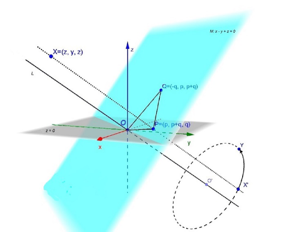
Figure 1: The operator $\boldsymbol{j}$ rotates plane $M$ by $\frac{\pi}{3}$ radians since $\boldsymbol{\mathbf{\boldsymbol{\mathbf{\mathit{P}}}}\boldsymbol{O}}\mathbf{\mathit{\boldsymbol{Q}}\,}$ is an equilateral triangle

1.3 Definition and properties of the $\circledast$-product

We are ready to define the novel multiplication of $J_{3}$-numbers. Bearing in mind the multiplication rule for complex numbers and using (1.2), (1.6), and (1.7) we suggest the following

Definition 3. The $\circledast$-product of $J_{3}$-numbers

$$\boldsymbol{\boldsymbol{T}}=a+\boldsymbol{j}b+\boldsymbol{j}\boldsymbol{j}c,\>\boldsymbol{\boldsymbol{S}}=u+\boldsymbol{j}v+\boldsymbol{j}\boldsymbol{j}w\$$

is defined as

$$\begin{matrix}\boldsymbol{\boldsymbol{T}}\circledast\,\boldsymbol{\boldsymbol{S}}=&(au-bw-cv)+\boldsymbol{j}(av+bu-cw)+\boldsymbol{j}\boldsymbol{j}(aw+bv+cu).\end{matrix}\$$

The right hand side of (1.13) is in the form of a $J_{3}$-number, thus $\circledast$-multiplication is a closed operation. Moreover, it is easily checked to be commutative:

$$\begin{matrix}\boldsymbol{\boldsymbol{S}}\circledast\mathit{\boldsymbol{\boldsymbol{T}}}=\boldsymbol{T}\circledast\boldsymbol{\boldsymbol{S}},\end{matrix}\$$

and associative:

$$(\boldsymbol{\boldsymbol{S}}\circledast\mathit{\boldsymbol{\boldsymbol{T}}})\circledast\boldsymbol{U}=\boldsymbol{\boldsymbol{S}}\circledast\,(\mathit{\boldsymbol{\boldsymbol{T}}}\circledast\boldsymbol{U}).\$$

It is also straightforward to check that all the axioms of the commutative unital associative algebra over $\mathbb{\mathbf{\mathbb{R}}}$ hold true for the $\circledast$-multiplication and component-wise addition of $J_{3}$-numbers, with zero $\mathbf{0}$ and $\circledast$-multiplicative unity $\mathbf{1}$ given by formulas (1.3.0) and (1.3.1), respectively. In particular, for any $\boldsymbol{\boldsymbol{S}}\in\mathbb{\mathbf{\mathbb{R}}}^{3}$:

$$\boldsymbol{\boldsymbol{S}}+\mathbf{0}=\mathbf{0}+\boldsymbol{\boldsymbol{S}}=\boldsymbol{\boldsymbol{S}},\quad\boldsymbol{\boldsymbol{S}}+(-\boldsymbol{\boldsymbol{S}})=\boldsymbol{0}$$

$$\boldsymbol{\boldsymbol{S}}\circledast\mathbf{\mathbf{1}}=\mathbf{\mathbf{1}}\circledast\,\mathit{\boldsymbol{\boldsymbol{S}}=\boldsymbol{\boldsymbol{S}}},\$$

$$\boldsymbol{\boldsymbol{S}}\circledast\mathbf{\mathbf{0}}=\mathbf{\mathbf{0}}\circledast\,\mathit{\boldsymbol{\boldsymbol{S}}=\mathbf{\mathbf{0}.}}$$

We will denote this commutative unital associative algebra over $\mathbb{\mathbf{\mathbb{R}}}$ equipped with the $\circledast$-product by $\mathbb{\mathbf{\mathbb{R}}}_{\circledast}^{3}$ or simply by $\mathbb{\mathbf{\mathbb{R}}}^{3}$.

Let us also note that any real number $r$ could be uniquely represented as a $J_{3}$-number with second and third components being equal to zero:

$$r\rightarrow\mathbf{r}=(r,\,0,\,0)=r\,+\boldsymbol{j}0\,+\boldsymbol{j}\boldsymbol{j}0,$$

and that the $\circledast$-product of such $J_{3}$-numbers by (1.13) reduces to the usual multiplication of real numbers: $\mathbf{r_{1}\circledast r_{2}}=r_{1}\,r_{2}.$ In view of (1.3.1) this means that $\mathbb{\mathbf{\mathbb{R}}}$ is a unital subalgebra of $\mathbb{\mathbf{\mathbb{R}}}^{3}$ and the above $r\rightarrow\mathbf{r}$ mapping is a unital algebra homomorphism.

The $\circledast$-multiplication table for the standard basis $\{\boldsymbol{e_{1},\,e_{2},\,e_{3}}\}\,$ of the above algebra $\mathbb{\mathbf{\mathbb{R}}}^{3}$ looks as follows:

$\boldsymbol{\circledast}$	$\boldsymbol{e_{1}}$	$\boldsymbol{e_{2}}$	$\boldsymbol{e_{3}}$
$\boldsymbol{e_{1}}$	$\boldsymbol{e_{1}}$	$\boldsymbol{e_{2}}$	$\boldsymbol{e_{3}}$
$\boldsymbol{e_{2}}$	$\boldsymbol{e_{2}}$	$\boldsymbol{e_{3}}$	-$\boldsymbol{e_{1}}$
$\boldsymbol{e_{3}}$	$\boldsymbol{e_{3}}$	-$\boldsymbol{e_{1}}$	-$\boldsymbol{e_{3}}$

$$\mathbf{\mathbf{Table}\>1}$$

The major property of the $\circledast$-multiplication is given by the following

Lemma 3. The $\boldsymbol{j}$-invariant subspaces $L\,$ and $M$ are mutually $\circledast$-orthogonal.

Proof. Let us take arbitrary $J_{3}$-numbers $\boldsymbol{\boldsymbol{L=}}(l,-l,\,l),\;\boldsymbol{\boldsymbol{M=}}(m,\,m+n,\,n)\,$ that belong to $L\,$ and $M,$ respectively. One can see that $L\,$ and $M$ might be represented as follows:

$$\boldsymbol{\boldsymbol{L=}}l\,(1-\boldsymbol{j}+\boldsymbol{j}\boldsymbol{j}),\,\boldsymbol{M}=(1+\boldsymbol{j})\circledast(m+\boldsymbol{j}n).$$

The direct calculations show that

$$\boldsymbol{\boldsymbol{L}\circledast}\,\boldsymbol{\boldsymbol{M}}=l\,(1-\boldsymbol{j}+\boldsymbol{j}\boldsymbol{j})\circledast(1+\boldsymbol{j})\circledast(m+\boldsymbol{j}n)=l\,(1+\boldsymbol{j}^{3})\circledast(m+\boldsymbol{j}n)=\boldsymbol{0},$$

where the last equality is justified by (1.2). □

1.4 Ideals in $\mathbb{\mathbf{\mathbb{R}}}^{3}$

The above results imply that both $L\,$ and $M$ are closed under the addition, subtraction and $\circledast$-multiplication of $J_{3}$-numbers, i.e., both are subalgebras of $\mathbb{\mathbf{\mathbb{R}}}^{3}$. Moreover, they turn out to be ideals of the real algebra $\mathbb{\mathbf{\mathbb{R}}}^{3}$ due to their absorbing (or ideal) property:

$$\forall\boldsymbol{\boldsymbol{S}}\!\in\!\mathbb{\mathbf{\mathbb{R}}}^{3},\>\forall\!\boldsymbol{M\!\in\!}M,\>\forall\!\boldsymbol{L\!\in\!}L:\;\boldsymbol{\boldsymbol{S}}\circledast\boldsymbol{M\!\in\!}M,\>\boldsymbol{\boldsymbol{S}}\circledast\boldsymbol{L\!\in\!}L,$$

which is obvious in view of Lemma 3. The above inclusions might be written down in a compact form as follows:

$$\mathbb{\mathbf{\mathbb{R}}}^{3}\circledast M\subset M,\;\mathbb{\mathbf{\mathbb{R}}}^{3}\circledast L\subset L.$$

1.5 Zero divisors and $\circledast$-invertibility

Definition 4. $J_{3}$-number $\boldsymbol{\boldsymbol{S}}$ is called $\circledast$-invertible in $\mathbb{\mathbf{\mathbb{R}}}^{3}$ if there exists another $J_{3}$-number called $\circledast$-inverse of $\boldsymbol{\boldsymbol{S}}$ and denoted by $\boldsymbol{\boldsymbol{S}}^{\boldsymbol{\mathrm{-1}}}$ such that

$$\boldsymbol{\boldsymbol{S}}^{-1}\circledast\,\boldsymbol{\boldsymbol{S}}=\boldsymbol{\boldsymbol{S}}\circledast\,\boldsymbol{\boldsymbol{S}{}^{\mathrm{-1}}}=\boldsymbol{1}.\$$

Lemma 4. Let $u,\,v,\,w\,$ be real numbers such that $\Delta=u^{3}-v^{3}+w^{3}+3uvw\neq 0$.

Then $\>\mathbf{\mathbf{\mathit{\boldsymbol{\boldsymbol{S}}}=}}u+\boldsymbol{j}v+\boldsymbol{j}\boldsymbol{j}w\;$ is $\,\circledast$-invertible and its $\,\circledast$-inverse $\boldsymbol{\boldsymbol{S}}^{-1}$ is given by

$$\boldsymbol{\boldsymbol{S}}^{-1}=\frac{u^{2}+vw}{\Delta}+\boldsymbol{j}\frac{-w^{2}-uv}{\Delta}+\boldsymbol{j}\boldsymbol{j}\frac{v^{2}-uw}{\Delta}.\$$

Proof. Let us rewrite the linear equation $\mathit{\boldsymbol{\boldsymbol{S}}\circledast\boldsymbol{\!X=}}\boldsymbol{1}$ for an unknown $J_{3}$-number $\boldsymbol{X}\mathbf{\mathbf{=}}\,x+\boldsymbol{j}y+\boldsymbol{j}\boldsymbol{j}z$ in the following form:

$$(ux-wy-vz)+\boldsymbol{j}(vx+uy-wz)+\boldsymbol{j}\boldsymbol{j}(wx+vy+uz)=1\,+\boldsymbol{j}0\,+\boldsymbol{j}\boldsymbol{j}0.$$

By matching the corresponding components this might be rewritten as

$$\left(\begin{matrix}u&-w&-v\\ v&u&-w\\ w&v&u\end{matrix}\right)\;\left(\begin{matrix}x\\ y\\ z\end{matrix}\right)=\left(\begin{matrix}1\\ 0\\ 0\end{matrix}\right).$$

To complete the proof it is enough to check that the expression $\Delta=\Delta(u,v,w)$ is a determinant of the Toeplitz matrix

$$T=\left(\begin{matrix}u&-w&-v\\ v&u&-w\\ w&v&u\end{matrix}\right)\$$

and to invoke the Cramer’s rule. □

Remark. An intimate connection between $J_{3}$-numbers and Toeplitz matrices of the form (1.19) will be established below, in Subsection 2.2.

Definition 5. A nonzero $J_{3}$-number $\boldsymbol{\boldsymbol{S}}\neq\mathbf{0}$ is called a zero divisor if there exists $\boldsymbol{\boldsymbol{T}}\neq\mathbf{0}$ in $\mathbb{\mathbf{\mathbb{R}}}^{3}$ such that

$$\boldsymbol{\boldsymbol{S}}\boldsymbol{\circledast}\boldsymbol{\boldsymbol{T}=}\mathbf{0.}\$$

We will refer to a pair of non-zero $J_{3}$-numbers that satisfy (1.20) as the dual zero divisors. The full characterization of zero divisors in $\mathbb{\mathbf{\mathbb{R}}}^{3}$ and $\circledast$-invertible $J_{3}$-numbers is given below.

Theorem 1.2. Let $\,\mathbf{\mathbf{\mathit{\boldsymbol{\boldsymbol{S}}}=}}u+\boldsymbol{j}v+\boldsymbol{j}\boldsymbol{j}w\neq\boldsymbol{0,}\,$ be a $J_{3}$-number. The following statements are equivalent:

1. The components of $\mathbf{\mathbf{\mathit{\boldsymbol{\boldsymbol{S}}}}}$ satisfy the equation:

   $$u^{3}-v^{3}+w^{3}+3uvw=0.\$$

2. $\mathbf{\mathbf{\mathit{\boldsymbol{\boldsymbol{S}}}}}$ belongs to either one of the $\boldsymbol{j}$-invariant subspaces $L\,$ and $M$.

3. $\mathbf{\mathbf{\mathit{\boldsymbol{\boldsymbol{S}}}}}$ is a zero divisor.

4. $\mathbf{\mathbf{\mathit{\boldsymbol{\boldsymbol{S}}}}}$ is not $\circledast$-invertible.

Proof. We are going to show that 1$\Rightarrow$ 2$\Rightarrow$ 3 $\Rightarrow$ 4 $\Rightarrow$1.

1 $\Rightarrow$2  The following easy-to-check identity

$$u^{3}-v^{3}+w^{3}+3uvw=\frac{1}{2}(u-v+w)\,\cdot((u+v)^{2}+(u-w)^{2}+(v+w)^{2})$$

implies that under (1.21) either $u-v+w=0,$ or $\;(u+v)^{2}+(u-w)^{2}+(v+w)^{2}=0,$ which means that $\,\boldsymbol{\boldsymbol{S}}$ belongs to either $M$ or $L$ as defined by (1.10) or (1.8), respectively.

2 $\Rightarrow$ 3  It follows from Lemma 3 that each point of the $\boldsymbol{j}$-invariant subspaces $L\,$ and $M\,$ ($\,\mathbf{0}$ excluded) is a zero divisor.

3 $\Rightarrow$4  Let us suppose that $\,\boldsymbol{\boldsymbol{S}}$ is both a zero divisor and $\circledast$-invertible in $\mathbb{\mathbf{\mathbb{R}}}^{3}\,$ and take an arbitrary $J_{3}$-number $\boldsymbol{\boldsymbol{T}}$ such that $\boldsymbol{\boldsymbol{S}}\boldsymbol{\circledast}\,\boldsymbol{\boldsymbol{\boldsymbol{T}}=}\mathbf{0}$. Then, in view of (1.15), (1.16), and (1.17), $\boldsymbol{\boldsymbol{T}}$ would also satisfy:

$$\boldsymbol{\boldsymbol{\boldsymbol{T}}=(\boldsymbol{\boldsymbol{S}}{}^{\boldsymbol{\mathrm{-1}}}\circledast\,\boldsymbol{\boldsymbol{S}})}\circledast\mathit{\boldsymbol{\boldsymbol{T}}}=\boldsymbol{\boldsymbol{\boldsymbol{S}}{}^{\boldsymbol{\mathrm{-1}}}\circledast\>(\boldsymbol{\boldsymbol{S}}}\circledast\mathit{\boldsymbol{\boldsymbol{T}})=\boldsymbol{\boldsymbol{S}}{}^{\boldsymbol{\mathrm{-1}}}\circledast\,}\boldsymbol{0=0.}$$

Thus, $\boldsymbol{\boldsymbol{T}}=0$ which contradicts the assumption that $\,\mathbf{\mathbf{\mathit{\boldsymbol{\boldsymbol{S}}}}}$ is a zero divisor.

4 $\Rightarrow$1  Suppose that (1.21) does not hold. Then Lemma 4 implies that $\mathbf{\mathbf{\mathit{\boldsymbol{\boldsymbol{S}}}}}$ is $\circledast$-invertible which contradicts the assumption 4.

This completes the proof of the theorem. □

Lemma 5. The modulus of the $\circledast$-product of $\boldsymbol{\boldsymbol{S}}$ and $\boldsymbol{\boldsymbol{T}}$ satisfies the following important inequality:

$$|\boldsymbol{\boldsymbol{S}}\circledast\mathit{\boldsymbol{\boldsymbol{T}}}|\leq\sqrt{3}\cdot|\boldsymbol{\boldsymbol{S}}|\,|\mathit{\boldsymbol{\boldsymbol{T}}}|.\$$

Proof. Let us observe that by direct calculations using (1.4) and (1.13) one has:

$$|\boldsymbol{\boldsymbol{S}}\circledast\mathit{\boldsymbol{\boldsymbol{T}}}|^{2}=|\boldsymbol{\boldsymbol{S}}|^{2}\,|\mathit{\boldsymbol{\boldsymbol{T}}}|^{2}+2\left\{\boldsymbol{\boldsymbol{S}}\right\}\left\{\boldsymbol{\boldsymbol{T}}\right\},$$

where $\left\{\mathbf{\mathbf{\mathit{\boldsymbol{\boldsymbol{S}}}}}\right\}=uv-uw+vw,\;\left\{\boldsymbol{\boldsymbol{T}}\right\}=ab-ac+bc.$ On the other hand, an obvious inequality

$$(u+v)^{2}+(u-w)^{2}+(v+w)^{2}\geq 0$$

is equivalent to $uv-uw+vw\leq u^{2}+v^{2}+w^{2}$and, therefore, $\left\{\mathbf{\mathbf{\mathit{\boldsymbol{\boldsymbol{S}}}}}\right\}\leq\,|\boldsymbol{\boldsymbol{S}}|^{2}$, $\left\{\boldsymbol{\boldsymbol{T}}\right\}\leq\,|\boldsymbol{\boldsymbol{T}}|^{2}$. Thus, $|\boldsymbol{\boldsymbol{S}}\circledast\mathit{\boldsymbol{\boldsymbol{T}}}|^{2}\leq 3|\boldsymbol{\boldsymbol{S}}|^{2}\,|\mathit{\boldsymbol{\boldsymbol{T}}}|^{2}$ and the rest is plain. □

Remark. It follows from Lemma 5 that the Hamilton’s law of moduli $|\boldsymbol{\boldsymbol{S}}\circledast\mathit{\boldsymbol{\boldsymbol{T}}}|=|\boldsymbol{\boldsymbol{S}}|\,|\mathit{\boldsymbol{\boldsymbol{T}}}|$ holds true if and only if at least one of $\boldsymbol{\boldsymbol{S}}$ or $\boldsymbol{\boldsymbol{T}}$ belongs to the infinite elliptic cone $xy-xz+yz=0$.

Lemma 6. Dual zero divisors belong to different $\boldsymbol{j}$-invariant subspaces.

Proof. First, suppose that the dual zero divisors $\boldsymbol{\boldsymbol{L_{1}}}$ and $\boldsymbol{\boldsymbol{L_{2}}}$ belong to the same $\boldsymbol{j}$-invariant subspace $L\,$, i.e. $\boldsymbol{\boldsymbol{L_{1}}}=l_{1}(1-\boldsymbol{j}+\boldsymbol{j}\boldsymbol{j})$ and $\boldsymbol{\boldsymbol{L_{2}}}=l_{2}(1-\boldsymbol{j}+\boldsymbol{j}\boldsymbol{j})$ for some non-zero real $l_{1},\,l_{2}.$ It is easy to see that

$$\boldsymbol{\boldsymbol{L_{1}}}\circledast\boldsymbol{\boldsymbol{L_{2}}}=3\,l_{1}\,l_{2}(1-\boldsymbol{j}+\boldsymbol{j}\boldsymbol{j})=\boldsymbol{0}\$$

implies that at least one of $l_{1}\,.$ or $l_{2}$ vanishes, which contradicts the assumption that both $\boldsymbol{\boldsymbol{L_{1}}}$ and $\boldsymbol{\boldsymbol{L_{2}}}$ are zero divisors.

Now let us take two arbitrary non-zero $J_{3}$-numbers $\boldsymbol{\boldsymbol{M_{1}}}=(m_{1},\,m_{1}+n_{1},\,n_{1})$ and $\boldsymbol{\boldsymbol{M_{2}}}=(m_{2},\,m_{2}+n_{2},\,n_{2})$ from the same $\boldsymbol{j}$-invariant subspace $M$.

By Lemma 5 the squared modulus of their $\circledast$-product is equal to:

$$\boldsymbol{|\boldsymbol{M_{1}}}\circledast\boldsymbol{\boldsymbol{M_{2}}}|^{2}=\boldsymbol{|\boldsymbol{M_{1}}}|^{2}|\boldsymbol{\boldsymbol{M_{2}}}|^{2}+\boldsymbol{2}\,\left\{\boldsymbol{\boldsymbol{M_{1}}}\right\}\,\left\{\boldsymbol{\boldsymbol{M_{2}}}\right\}=\frac{3}{2}\boldsymbol{|\boldsymbol{M_{1}}}|^{2}|\boldsymbol{\boldsymbol{M_{2}}}|^{2},$$

where the last equality holds true since

$$\left\{\boldsymbol{\boldsymbol{M}_{i}}\right\}=m_{i}(m_{i}+n_{i})-m_{i}n_{i}+(m_{i}+n_{i})n_{i}=m_{i}^{2}+m_{i}n_{i}+n_{i}^{2}=\frac{1}{2}\boldsymbol{|\boldsymbol{M}_{i}}|^{2}.$$

As $\boldsymbol{\boldsymbol{M_{1}}}$ and $\boldsymbol{\boldsymbol{M_{2}}}$ are assumed to be non-zero their moduli $|\boldsymbol{M_{1}}|$ and $|\boldsymbol{M_{2}}|$ are both positive. Thus, one has $|\boldsymbol{\boldsymbol{M_{1}}}\circledast\boldsymbol{\boldsymbol{M_{2}}}|>0$ and consequently $\boldsymbol{\boldsymbol{M}_{1}}\circledast\boldsymbol{\boldsymbol{M_{2}}}\neq\boldsymbol{0}$, i.e., $\boldsymbol{\boldsymbol{M_{1}}}$ and $\boldsymbol{\boldsymbol{M_{2}}}$ are not dual zero divisors. □

1.6 Linear equations in $\mathbb{\mathbf{\mathbb{R}}}^{3}$

The existence of zero divisors implies that $\mathbb{\mathbf{\mathbb{R}}}^{3}$ is not a field, i.e., the division is not always possible. Still, when $\boldsymbol{\boldsymbol{S}}$ is $\circledast$-invertible and $\boldsymbol{\boldsymbol{T}}$ is an arbitrary $J_{3}$-number then there exists $\boldsymbol{X}=\boldsymbol{\boldsymbol{S}}{}^{\boldsymbol{\mathrm{-1}}}\circledast\,\boldsymbol{\boldsymbol{T}}$ such that:

$$\boldsymbol{\boldsymbol{\boldsymbol{S}}\circledast X=\boldsymbol{\boldsymbol{T}}.}\$$

We have already characterized in Theorem 1.2 all the $\circledast$-invertible $J_{3}$-numbers. Now we are going to investigate under what conditions the linear equation (1.24) is solvable in $\mathbb{\mathbf{\mathbb{R}}}^{3}.$

Lemma 7. Let both $\boldsymbol{\boldsymbol{T}}=t-\boldsymbol{j}t+\boldsymbol{j}\boldsymbol{j}t\,$ and $\>\boldsymbol{\boldsymbol{S}}=s-\boldsymbol{j}s+\boldsymbol{j}\boldsymbol{j}s\neq\boldsymbol{0\,}$ belong to the $\boldsymbol{j}$-invariant subspace $L.$ Then the equation (1.24) has a unique solution in $L$:

$$\boldsymbol{X}_{L}=\frac{t}{3s}\,(1-\boldsymbol{j}+\boldsymbol{j}\boldsymbol{j})$$

and infinitely many solutions in $\mathbb{\mathbf{\mathbb{R}}}^{3}:$

$$\boldsymbol{X}=\boldsymbol{X}_{L}+\boldsymbol{X}_{M},$$

where $\boldsymbol{X}_{M}$ is an arbitrary $J_{3}$-number from the $\boldsymbol{j}$-invariant subspace $M.$

Proof. The uniqueness and the formula for $\boldsymbol{X}_{L}$ follows directly from (1.23). The rest is easy due to Lemmas 3 and 6. □

Lemma 8. Let both $\boldsymbol{\boldsymbol{S}}=u+\boldsymbol{j}(u+v)+\boldsymbol{j}\boldsymbol{j}v\neq\boldsymbol{0}\,$ and $\boldsymbol{\boldsymbol{T}}=a+\boldsymbol{j}(a+b)+\boldsymbol{j}\boldsymbol{j}b$ belong to the $\boldsymbol{j}$-invariant subspace $M.$ Then the equation (1.24) has a unique solution in the plane $M$:

$$\boldsymbol{X}_{M}=c+\boldsymbol{j}(c+d)+\boldsymbol{j}\boldsymbol{j}d,$$

$$c=\frac{u\,(2a+b)+v\,(a+2b)}{3(u^{2}+uv+v^{2})},\,d=\frac{u\,(a-b)+v\,(2a+b)}{3(u^{2}+uv+v^{2})}$$

and infinitely many solutions in $\mathbb{\mathbf{\mathbb{R}}}^{3}:$

$$\boldsymbol{X}=\boldsymbol{X}_{L}+\boldsymbol{X}_{M},$$

where $\boldsymbol{X}_{L}$ is an arbitrary $J_{3}$-number from the $\boldsymbol{j}$-invariant subspace $L.$

Proof. Let us $\circledast$-multiply $\boldsymbol{\boldsymbol{S}}=u+\boldsymbol{j}(u+v)+\boldsymbol{j}\boldsymbol{j}v$ by $\boldsymbol{X}_{M}=c+\boldsymbol{j}(c+d)+\boldsymbol{j}\boldsymbol{j}d$ and compare the product to $\boldsymbol{\boldsymbol{T}}=a+\boldsymbol{j}(a+b)+\boldsymbol{j}\boldsymbol{j}b.$ By matching the corresponding coefficients we get a real linear system of 3 equations with 2 real unknown variables where one equation is a linear combination of two others. After reducing this system to 2-by-2 case its determinant happens to be proportional to $u^{2}+uv+v^{2}\neq 0.$ Then the formula for the solution in the plane $M$ is a consequence of Cramer’s rule. Now it is enough to invoke Lemmas 3 and 6 in order to complete the proof. □

We are going to summarize the above discussion in the following

Theorem 1.3. Let $\boldsymbol{\boldsymbol{S}}\neq\boldsymbol{0}$ and $\boldsymbol{\boldsymbol{T}}$ be $J_{3}$-numbers. Then the linear equation

$$\boldsymbol{\boldsymbol{\boldsymbol{S}}\circledast X=\boldsymbol{\boldsymbol{T}}.}\$$

1) has a unique solution in $\mathbb{\mathbf{\mathbb{R}}}^{3}$ if $\boldsymbol{\boldsymbol{S}}\,$ is $\circledast$-invertible;

2) has no solution in $\mathbb{\mathbf{\mathbb{R}}}^{3}$ if

(a) $\boldsymbol{\boldsymbol{T}}$ is $\circledast$-invertible while $\boldsymbol{\boldsymbol{S}}\,$ is a zero divisor, or

(b) $\boldsymbol{\boldsymbol{S}}\,$ and $\boldsymbol{\boldsymbol{T}}$ are dual zero divisors;

3) has infinitely many solutions in $\mathbb{\mathbf{\mathbb{R}}}^{3}$ if

(a) both $\boldsymbol{\boldsymbol{S}}\,$ and $\boldsymbol{\boldsymbol{T}}$ are (non-dual) zero divisors, such that $\boldsymbol{\boldsymbol{S}}\circledast\mathit{\boldsymbol{\boldsymbol{T}}}\neq\boldsymbol{0}$, or

(b) $\boldsymbol{\boldsymbol{S}}\,$ is a zero divisor while $\boldsymbol{\boldsymbol{T}}=\boldsymbol{0}$.

Proof. 1) Given $\boldsymbol{\boldsymbol{S}}\,$ is $\circledast$-invertible, let us take a $J_{3}$-number $\boldsymbol{X}=\boldsymbol{\boldsymbol{S}}{}^{\boldsymbol{\mathrm{-1}}}\circledast\,\boldsymbol{\boldsymbol{T}}.$

It follows from (1.16), (1.17), and the associativity of the $\circledast$-multiplication that $\boldsymbol{X}$ is a solution of (1.24). If $\boldsymbol{Y}\in\mathbb{\mathbf{\mathbb{R}}}^{3}$ is also a solution, i.e., $\boldsymbol{\boldsymbol{S}}\circledast\boldsymbol{Y}=\boldsymbol{\boldsymbol{T}}$ then

$$\boldsymbol{Y}=(\boldsymbol{\boldsymbol{S}}{}^{\boldsymbol{\mathrm{-1}}}\circledast\boldsymbol{\boldsymbol{S}})\circledast\boldsymbol{Y}=\boldsymbol{\boldsymbol{S}}{}^{\boldsymbol{\mathrm{-1}}}\circledast(\boldsymbol{\boldsymbol{S}}\circledast\boldsymbol{Y})=\boldsymbol{\boldsymbol{S}}{}^{\boldsymbol{\mathrm{-1}}}\circledast\boldsymbol{\boldsymbol{T}}=\boldsymbol{X}.$$

2a) Assume there exists a solution $\boldsymbol{X}$ of the linear equation $\boldsymbol{\boldsymbol{\boldsymbol{S}}\circledast X=\boldsymbol{\boldsymbol{T}}}$ where $\boldsymbol{\boldsymbol{T}}$ is $\circledast$-invertible and $\boldsymbol{\boldsymbol{S}}\,$ is a zero divisor. By setting $\mathit{\boldsymbol{X}}_{1}=\boldsymbol{X}\circledast\boldsymbol{\boldsymbol{T}}^{-1}$one has:

$$\boldsymbol{\boldsymbol{S}}\circledast\boldsymbol{X}_{1}=\boldsymbol{\boldsymbol{S}}\circledast(\boldsymbol{X}\circledast\boldsymbol{\boldsymbol{T}}^{-1})=(\boldsymbol{\boldsymbol{S}}\circledast\boldsymbol{X})\circledast\boldsymbol{\boldsymbol{T}}^{-1}=\boldsymbol{1},$$

i.e., $\boldsymbol{\boldsymbol{S}}$ turns out to be $\circledast$-invertible which contradicts Theorem 1.2.

2b) Now assume that for some $J_{3}$-number $\boldsymbol{X}$ the equation (1.24) holds true with $\boldsymbol{\boldsymbol{S}}\,$ and $\boldsymbol{\boldsymbol{T}}$ being dual zero divisors.

Let us observe that by Lemma 6 the $J_{3}$-numbers $\boldsymbol{\boldsymbol{S}}\,$ and $\boldsymbol{\boldsymbol{T}}$ belong to different $\boldsymbol{j}$-invariant subspaces. Since $L\,$ and $M$ are ideals in $\mathbb{\mathbf{\mathbb{R}}}^{3}$ (see Subsection 1.4), the left hand side $\boldsymbol{\boldsymbol{\boldsymbol{S}}\circledast X}$ belongs to the same $\boldsymbol{j}$-invariant subspace as $\boldsymbol{\boldsymbol{S}}\,$ and could meet the right hand side $\boldsymbol{\boldsymbol{T}}$ of (1.24) only at $\boldsymbol{0}$. This contradicts the assumption that, as a zero divisor, $\boldsymbol{\boldsymbol{T}}\neq\boldsymbol{0}$.

3) This claim is plain from Lemmas 6, 7 and 8. □

1.7 Square roots of unity and idempotents in $\mathbb{\mathbf{\mathbb{R}}}^{3}$

Since the $\circledast$-multiplication is a closed operation in $\mathbb{\mathbf{\mathbb{R}}}^{3}$ we could define the square of a $J_{3}$-number as the $\circledast$-product of $\boldsymbol{\boldsymbol{S}}=u+\boldsymbol{j}v+\boldsymbol{j}\boldsymbol{j}w\,$ with itself:

$$\boldsymbol{\boldsymbol{S}^{2}}\overset{def}{=}\boldsymbol{\boldsymbol{S}}\circledast\mathit{\boldsymbol{\boldsymbol{S}}.}$$

Theorem 1.4. Let $r$ be a real number. Then the quadratic equation in $\mathbb{\mathbf{\mathbb{R}}}^{3}$:

$$\boldsymbol{X^{2}=}r\$$

1) has no solution if $r<0$ ,

2) has a unique solution $\boldsymbol{X}=\mathbf{0\,}$ if $\,r=0$,

3) has exactly $4$ distinct solutions if $\,r>0$.

Proof. It is easy to check by direct calculations based on (1.12), (1.13) that

$$\boldsymbol{\boldsymbol{S}^{2}}=(u^{2}-2vw)+\boldsymbol{j}(2uv-w^{2})+\boldsymbol{j}\boldsymbol{j}(v^{2}+2uw).\$$

Let us assume that $\boldsymbol{\boldsymbol{S}}\,$ is a solution of (1.25), i.e, $\boldsymbol{\boldsymbol{S}^{2}}=r+\boldsymbol{j}0+\boldsymbol{j}\boldsymbol{j}0$:

$$u^{2}-2vw=r,\;2uv-w^{2}=0,\;v^{2}+2uw=0.\$$

It follows that:

$$r=(u^{2}-2vw)-(2uv-w^{2})+(v^{2}+2uw)=(u-v+w)^{2}\geq 0.\$$

This means that the $\circledast$-square of a $J_{3}$-number cannot be equal to a negative real number which proves claim 1).

If $r=0$ the existence of a trivial solution $\boldsymbol{\boldsymbol{X}}=\mathbf{0\,}$ is easy. To prove its uniqueness let us assume that there exists an additional solution $\boldsymbol{\boldsymbol{S}}\neq\boldsymbol{0}$ of (1.25):

$$\boldsymbol{\boldsymbol{S}}\circledast\mathit{\boldsymbol{\boldsymbol{S}}}=\mathbf{0.}$$

By Lemma 6 this implies $\boldsymbol{\boldsymbol{S}}=\boldsymbol{0}$, as it should belong to both $\boldsymbol{j}$-invariant subspaces $L\,$ and $M$. The contradiction proves 2).

Finally, let us consider the remaining case when $\,r>0.$ It is easy to see from (1.27) that $\,v\,$ and $\,w\,$ are either both $0,$ or both non-zero. If $v=w=0$ one has $u^{2}=r,\;$ which gives us two expected real roots: $\pm(\sqrt{r},\;0,\;0).$ If both $\,v\,$ and $\,w\,$ are non-zero then it follows from (1.27) that $v^{2}w^{2}=-4u^{2}vw\Longleftrightarrow vw=-4u^{2}$ while (1.28) shows that $(u-v+w)^{2}=r,$ and the following system of equations with a positive parameter $r$ emerges:

$$9u^{2}=u^{2}-2vw=r,\;vw=-4u^{2}=-\frac{4r}{9},\;v-w=u\pm\sqrt{r}.\$$

By solving this system one obtains two additional solutions of (1.25) :

$$u=\epsilon\,\frac{\sqrt{r}}{3},\;v=\epsilon\,\frac{2\sqrt{r}}{3},\;w=-\epsilon\,\frac{2\sqrt{r}}{3},\;\epsilon=\pm 1,\$$

which completes the proof. □

Corollary 1. There are exactly 4 square roots of unity in $\mathbb{\mathbf{\mathbb{R}}}^{3}$:

$$\boldsymbol{1},\boldsymbol{-1},\,\frac{1}{3}(1+2\boldsymbol{j}-2\boldsymbol{j}\boldsymbol{j}),\,-\frac{1}{3}(1+2\boldsymbol{j}-2\boldsymbol{j}\boldsymbol{j}).\$$

Proof. The roots $\boldsymbol{1},\boldsymbol{-1}$ are trivial, the other two are obtained from (1.30) by setting $\,r=1$. □

Corollary 2. There are exactly 4 idempotents of algebra $\mathbb{\mathbf{\mathbb{R}}}^{3}$:

$$\boldsymbol{0},\,\boldsymbol{1},\,\frac{1}{3}(1-\boldsymbol{j}+\boldsymbol{j}\boldsymbol{j}),\,\frac{1}{3}(2+\boldsymbol{j}-\boldsymbol{j}\boldsymbol{j})\$$

Proof. Let us use the substitution $\boldsymbol{\boldsymbol{X}}=\boldsymbol{\boldsymbol{Y}}+\dfrac{1}{2}$ to rewrite the idempotence equation

$$\boldsymbol{\boldsymbol{X}\circledast\boldsymbol{X}=}\boldsymbol{\boldsymbol{X}}\$$

in the form of (1.25):

$$\boldsymbol{\boldsymbol{Y}}^{2}=\frac{1}{4}.$$

Then it is easily seen that its real roots $\boldsymbol{\boldsymbol{Y}}=\pm\dfrac{1}{2}$ lead to trivial solutions of (1.33): $\boldsymbol{0}$ and $\boldsymbol{1}$, while the roots given by (1.30) produce

$$\boldsymbol{\boldsymbol{\alpha}=}\dfrac{1}{3}(1,\,-1,\,1),\;\boldsymbol{\boldsymbol{\beta}=}\dfrac{1}{3}(2,\,1,\,-1),\$$

the two remaining solutions. □

Let us note that $\boldsymbol{\alpha}$ and $\boldsymbol{\beta}$ sum up to $\boldsymbol{1}$, belong to the $\boldsymbol{j}$-invariant subspaces $L\,$ and $M$, respectively, and their $\circledast$-product is equal to $\mathbf{0}$:

$$\boldsymbol{\boldsymbol{\alpha}=}\dfrac{1}{3}(1-\boldsymbol{j}+\boldsymbol{j}\boldsymbol{j})\in L,\$$

$$\boldsymbol{\boldsymbol{\beta}}=\dfrac{1}{3}(2+\boldsymbol{j}-\boldsymbol{j}\boldsymbol{j})\in M.\$$

$$\boldsymbol{\alpha}\circledast\boldsymbol{\boldsymbol{\beta}=0,\>\boldsymbol{\alpha}+\boldsymbol{\beta}=1.\ }$$

In particular, this leads to two different factorizations of the quadratic

polynomial $P(\boldsymbol{X})=\boldsymbol{X^{2}-}\boldsymbol{X}$ into linear factors:

$$P(\boldsymbol{X})=\boldsymbol{X}\circledast(\boldsymbol{X}-\boldsymbol{1})=(\boldsymbol{X}-\boldsymbol{\alpha})\circledast(\boldsymbol{X}-\boldsymbol{\beta}).\$$

1.8 New basis in $\mathbb{\mathbf{\mathbb{R}}}^{3}$ and the $\circledast$-multiplication table

Let us introduce now the following $J_{3}$-number

$$\boldsymbol{\boldsymbol{\gamma}}=\frac{\sqrt{3}}{3}(\boldsymbol{j}+\boldsymbol{j}\boldsymbol{j})\in M\$$

which is orthogonal, as a vector, to both $\boldsymbol{\alpha}$ and $\boldsymbol{\beta}$ and is $\circledast$-orthogonal to $\boldsymbol{\alpha}$ only. It is easy to check that

$$\boldsymbol{\beta}\circledast\boldsymbol{\boldsymbol{\gamma}}=\boldsymbol{\boldsymbol{\gamma}},\>\boldsymbol{\boldsymbol{\gamma}}\circledast\boldsymbol{\boldsymbol{\gamma}}=-\boldsymbol{\beta}\$$

The triple $\{\boldsymbol{\boldsymbol{\alpha}},\,\boldsymbol{\boldsymbol{\beta}},\,\boldsymbol{\boldsymbol{\boldsymbol{\gamma}}}\}$ is a new orthogonal (but not $\circledast$-orthogonal!) basis of $\mathbb{\mathbf{\mathbb{R}}}^{3}$ and the corresponding $\circledast$-multiplication table has a particularly neat form:

$\boldsymbol{\circledast}$	$\boldsymbol{\alpha}$	$\boldsymbol{\beta}$	$\boldsymbol{\boldsymbol{\gamma}}$
$\boldsymbol{\alpha}$	$\boldsymbol{\alpha}$	$\boldsymbol{0}$	$\boldsymbol{0}$
$\boldsymbol{\beta}$	$\boldsymbol{0}$	$\boldsymbol{\beta}$	$\boldsymbol{\boldsymbol{\gamma}}$
$\boldsymbol{\boldsymbol{\gamma}}$	$\boldsymbol{0}$	$\boldsymbol{\boldsymbol{\gamma}}$	-$\boldsymbol{\beta}$

$$\mathbf{\mathbf{Table}\>2}$$

A $J_{3}$-number $\mathbf{\mathbf{\mathit{\boldsymbol{\boldsymbol{S}}}=\,}}u+\boldsymbol{j}v+\boldsymbol{j}\boldsymbol{j}w$ in this basis would be represented as follows:

$$\boldsymbol{\boldsymbol{S}}=(u-v+w)\,\boldsymbol{\alpha}+\frac{1}{2}(2u+v-w)\,\boldsymbol{\beta}+\frac{\sqrt{3}}{2}(v+w)\,\boldsymbol{\boldsymbol{\gamma}},\$$

while a $J_{3}$-number $\mathbf{\mathbf{\mathit{\boldsymbol{\boldsymbol{T}}}=\,}}a\cdot\boldsymbol{\alpha}+b\cdot\boldsymbol{\beta}+c\cdot\boldsymbol{\boldsymbol{\gamma}}$ in the standard basis $\{\boldsymbol{e_{1},\,e_{2},\,e_{3}}\}$ has the following form:

$$\mathit{\boldsymbol{\boldsymbol{T}}}=\frac{a+2b}{3}+\boldsymbol{j}\frac{-a+b+c\cdot\sqrt{3}}{3}+\boldsymbol{j}\boldsymbol{j}\frac{a-b+c\cdot\sqrt{3}}{3}.\$$

It follows from (1.4) and (1.42) that the modulus of $\mathbf{\mathbf{\mathit{\boldsymbol{\boldsymbol{T}}}}}$ is equal to

$$|\boldsymbol{\boldsymbol{T}}|=|a\cdot\boldsymbol{\alpha}+b\cdot\boldsymbol{\beta}+c\cdot\boldsymbol{\boldsymbol{\gamma}}|=\sqrt{\frac{a^{2}+2b^{2}+2c^{2}}{3}}.\$$

1.9 Algebraic connection between $\mathbb{\mathbf{\mathbb{R}}}^{3}$ and $\mathbb{C}$

Our next objective is to establish an intimate algebraic connection between $J_{3}$-numbers and classical real and complex numbers. The block structure of the Table 2 hints that we should consider the direct sum of $\mathbb{\mathbf{\mathbb{R}}}$ and $\boldsymbol{\mathbb{C}}:$

$$\mathbf{\mathbf{\mathit{\boldsymbol{D}}}}=\mathbb{\mathbf{\mathbb{R}}}\oplus\boldsymbol{\mathbb{C}}=\{(r,\>\boldsymbol{z})\,|\,r\in\mathbb{\mathbf{\mathbb{R}}},\>\boldsymbol{z}\in\boldsymbol{\mathbb{C}}\}.\$$

Obviously, it would be a real 3D Euclidean space with addition and multiplication by a real scalar $k$ defined as

$$(r_{1},\,\boldsymbol{z}_{1})+(r_{2},\,\boldsymbol{z}_{2})=(r_{1}+r_{2},\,\boldsymbol{z}_{1}+\boldsymbol{z}_{2}),\quad k\,(r,\>\boldsymbol{z})=(k\,r,\>k\,\boldsymbol{z}).\$$

Let us introduce the product of the above pairs by the following rule:

$$(r_{1},\,\boldsymbol{z}_{1})\otimes(r_{2},\,\boldsymbol{z}_{2})=(r_{1}\,r_{2},\,\boldsymbol{z}_{1}\,\boldsymbol{z}_{2})\$$

with $\boldsymbol{z}_{1}\,\boldsymbol{z}_{2}=(x_{1}+\mathbf{i}\,y_{1})\,(x_{2}+\mathbf{i}\,y_{2})\,=(x_{1}x_{2}-y_{1}y_{2})+\mathbf{i}\,(x_{1}y_{2}+x_{2}y_{1})$ being the usual complex number multiplication. It is easily seen that the product (1.46) is bilinear and thus $\boldsymbol{D}$ becomes a unital commutative associative algebra over $\mathbb{\mathbf{\mathbb{R}}}$ with $\boldsymbol{1_{\boldsymbol{D}}=}(1,\,1+\mathbf{i}\,0)$ and $\boldsymbol{0_{\boldsymbol{D}}=}(0,\,0+\mathbf{i}\,0)$ being its unity and zero, respectively. Note that similarly to $\mathbb{\mathbf{\mathbb{R}}}^{3}$ the algebra $\boldsymbol{D}$ also has zero divisors: $(r,\,0)\otimes(0,\boldsymbol{\,z})=\boldsymbol{0}_{\boldsymbol{D}}\;\forall r\in\mathbb{\mathbf{\mathbb{R}}},\>\boldsymbol{\forall z}\in\boldsymbol{\mathbb{C}}.$

Now we are ready to establish the isomorphism between $\mathbb{\mathbf{\mathbb{R}}}^{3}$ and $\boldsymbol{D}$, all regarded as algebras over $\mathbb{\mathbf{\mathbb{R}}}$.

Theorem 1.5. $\mathbb{\mathbf{\mathbb{R}}}^{3}$ is isomorphic to the direct sum of $\mathbb{\mathbf{\mathbb{R}}}$ and $\boldsymbol{\mathbb{C}}$:

$$\mathbb{\mathbf{\mathbb{R}}}^{3}\cong\mathbb{\mathbf{\mathbb{R}}}\oplus\boldsymbol{\mathbb{C}.}\$$

Proof. Let us consider the following mapping $\Phi:\mathbb{\mathbf{\mathbb{R}}}^{3}\longmapsto\mathbb{\mathbf{\mathbb{R}}}\oplus\boldsymbol{\mathbb{C}}$ :

$$\boldsymbol{\boldsymbol{S}}=u+\boldsymbol{j}v+\boldsymbol{j}\boldsymbol{j}w=r\,\boldsymbol{\alpha}+x\,\boldsymbol{\beta}+y\,\boldsymbol{\boldsymbol{\gamma}}\longmapsto(r,\,x+\mathbf{i}\,y)=\Phi(\boldsymbol{\boldsymbol{S}}),\$$

where the real numbers $r,\,x,\,y$ are the components of $\boldsymbol{\boldsymbol{S}}$ in the basis $\{\boldsymbol{\boldsymbol{\alpha}},\,\boldsymbol{\boldsymbol{\beta}},\,\boldsymbol{\boldsymbol{\boldsymbol{\gamma}}}\}$:

$$r=u-v+w,\,x=\frac{1}{2}(2u+v-w),\,y=\frac{\sqrt{3}}{2}(v+w).\$$

First of all, formulas (1.41)-(1.42) show that this mapping is a bijection between $\mathbb{\mathbf{\mathbb{R}}}^{3}$ and $\boldsymbol{\mathbf{\mathbf{\mathit{\boldsymbol{D}}}}=\mathbb{\mathbf{\mathbb{R}}}\oplus\boldsymbol{\mathbb{C}}}$. Secondly, by using (1.48), (1.49) one can see that

$$\Phi(k_{1}\boldsymbol{\boldsymbol{S}}+k_{2}\boldsymbol{\boldsymbol{T}})=k_{1}\Phi(\boldsymbol{\boldsymbol{S}})+k_{2}\Phi(\boldsymbol{\boldsymbol{T}}),\;\forall k_{1},\,k_{2}\in\mathbb{\mathbf{\mathbb{R}}},\;\forall\boldsymbol{\boldsymbol{S}},\,\boldsymbol{\boldsymbol{T}}\in\mathbb{\mathbf{\mathbb{R}}}^{3},\$$

and that $\Phi$ maps the unity $\boldsymbol{1}$ of $\mathbb{\mathbf{\mathbb{R}}}^{3}$ into the unity of $\boldsymbol{D}$: $\Phi(\boldsymbol{1})=(1,1+\mathbf{i}0)=1_{\boldsymbol{D}}.$

Let us observe that by the very definition (1.48):

$$\Phi(\boldsymbol{\alpha})=\Phi(1\boldsymbol{\alpha}+0\boldsymbol{\beta}+0\boldsymbol{\boldsymbol{\gamma}})=(1,0),\,\Phi(\boldsymbol{\beta})=(0,1),\,\Phi(\boldsymbol{\boldsymbol{\gamma}})=(0,\mathbf{i}).\$$

It is an easy exercise now to show that the $\circledast$-multiplication Table 2 of Subsection 1.8 ensures

$$\Phi(\boldsymbol{\boldsymbol{S}}\circledast\boldsymbol{\boldsymbol{T}})=\Phi(\boldsymbol{\boldsymbol{S}})\otimes\Phi(\boldsymbol{\boldsymbol{T}}),\;\forall\boldsymbol{\boldsymbol{S}},\,\boldsymbol{\boldsymbol{T}}\in\mathbb{\mathbf{\mathbb{R}}}^{3},\$$

which completes the proof. □

The complex plane $\mathbb{C}$, as an algebra over $\mathbb{\mathbf{\mathbb{R}}}$, is isomorphic to the real subalgebra $M$ of $\mathbb{\mathbf{\mathbb{R}}}^{3}$. This could be seen from (1.48) where $r$ should be set to $0$ which induces an isomorphism

$$\Phi_{0}:\>M\longmapsto\mathbb{C}.\$$

Given $\boldsymbol{\boldsymbol{M=}}m+\boldsymbol{j}(m+n)+\boldsymbol{j}\boldsymbol{j}n\in M$, the corresponding complex number is $\Phi_{0}(\boldsymbol{M})=a+\mathbf{i}b$ with $a=\frac{3}{2}m$ and $b=(\frac{1}{2}m+n)\,\sqrt{3}$.

Given an arbitrary complex number $\boldsymbol{z=x+\mathbf{i}}y$, the corresponding $J_{3}$-number in $M$ could be computed by (1.42):

$$\Phi_{0}^{-1}(x+\mathbf{i}y)=0\,\boldsymbol{\alpha}+x\,\boldsymbol{\beta}+y\,\boldsymbol{\boldsymbol{\gamma}}=\frac{2x}{3}+\boldsymbol{j}\frac{x+y\cdot\sqrt{3}}{3}+\boldsymbol{j}\boldsymbol{j}\frac{-x+y\cdot\sqrt{3}}{3}.\$$

In particular, the complex unity $1_{\mathbb{C}}=(1,0)$ corresponds to the $J_{3}$-number $\boldsymbol{\beta}$ which is a unity of the real algebra $M$, while the imaginary unit $\mathbf{i}=(0,1)$ corresponds to $\boldsymbol{\boldsymbol{\gamma}}\!\in\!\mathbb{\mathbf{\mathbb{R}}}^{3}$.

We have observed earlier (see Subsection 1.3) that the algebra $\mathbb{\mathbf{\mathbb{R}}}^{3}$ contains $\mathbb{\mathbf{\mathbb{R}}}$ as a unital subalgebra. Does it similarly contains the real algebra of complex numbers? The answer is given by the following theorem.

Theorem 1.6. $\mathbb{C}$ is not a unital subalgebra of $\mathbb{\mathbf{\mathbb{R}}}^{3}.$

Proof. Let us assume that there exists a homomorphism $\Psi:\boldsymbol{\mathbb{C}}\longmapsto\mathbb{\mathbf{\mathbb{R}}}^{3}$ which maps the complex unity $1_{\mathbb{C}}$ into the unity $\boldsymbol{1}$ of $\mathbb{\mathbf{\mathbb{R}}}^{3}:$

$$\Psi(1+\mathbf{i}0)=\boldsymbol{1}.\$$

Let $\boldsymbol{\boldsymbol{S}}=\Psi(\mathbf{i})$ be the $\mathbb{\mathbf{\mathbb{R}}}^{3}$ image of $\mathbf{i}\in\mathbb{C}$. Then one has:

$$\Psi(1_{\mathbb{C}})=\Psi(-\mathbf{i}^{2})=-\Psi(\mathbf{i})\circledast\Psi(\mathbf{i})=-\boldsymbol{\boldsymbol{S}}\circledast\boldsymbol{\boldsymbol{S}}.\$$

On the other hand, it follows from Theorem 1.4 that

$$\boldsymbol{\boldsymbol{S}}^{2}\neq\boldsymbol{-1},\;\forall\boldsymbol{\boldsymbol{S}}\!\in\!\mathbb{\mathbf{\mathbb{R}}}^{3}.\$$

Therefore, $\Psi(1_{\mathbb{C}})$ is not equal to $\boldsymbol{1}$ which contradicts our assumption (1.54). □

1.10 Quadratic equations in $\mathbb{\mathbf{\mathbb{R}}}^{3}$

We are ready now to investigate the general quadratic equation with $J_{3}$-coefficients

$$\boldsymbol{\mathbf{\mathit{A}}}\circledast\boldsymbol{X}^{2}+\boldsymbol{\mathit{B}}\circledast\boldsymbol{X}+\boldsymbol{C}=\boldsymbol{0}.\$$

In what follows we are going to use the notion of the $J_{3}$-discriminant which is constructed similarly to the classical case:

Definition 6. The $J_{3}$-discriminant of the equation (1.57) is defined as

$$\boldsymbol{D}=\boldsymbol{B}^{2}-4\cdot\boldsymbol{A}\circledast\boldsymbol{C}.\$$

The following notion would also prove useful:

Definition 7. The altitude $|||\boldsymbol{\boldsymbol{S}}|||$ of the $J_{3}$-number $\boldsymbol{\boldsymbol{S}}=u+\boldsymbol{j}v+\boldsymbol{j}\boldsymbol{j}w$ is a real number defined as

$$|||\boldsymbol{\boldsymbol{S}}|||=u-v+w.\$$

Remark. Note that the mapping $\boldsymbol{\boldsymbol{S}}\rightarrow|||\boldsymbol{\boldsymbol{S}}|||$ is a real linear functional on $\mathbb{\mathbf{\mathbb{R}}}^{3}$. Besides, if $\boldsymbol{\boldsymbol{S}}=a\cdot\boldsymbol{\alpha}+b\cdot\boldsymbol{\beta}+c\cdot\boldsymbol{\boldsymbol{\gamma}}$ then by formula (1.49):

$$|||\boldsymbol{\boldsymbol{S}}|||=a.\$$

Let us also note that since the modulus $|\boldsymbol{\alpha}|=\frac{\sqrt{3}}{3}$, the altitude $|||\boldsymbol{\boldsymbol{S}}|||=a$ is equal to $\sqrt{3}$ times the oriented distance from the point $\boldsymbol{\boldsymbol{S}}\,$ to the $\boldsymbol{j}$-invariant plane $M$. Obviously, a $J_{3}$-number $\boldsymbol{\boldsymbol{S}}$ has a zero altitude if and only if $\boldsymbol{\boldsymbol{S}}\in M$.

Lemma 9. The altitude of the $\circledast$-product is equal to the product of altitudes:

$$|||\boldsymbol{\boldsymbol{S}}\circledast\boldsymbol{\boldsymbol{T}}|||=|||\boldsymbol{\boldsymbol{S}}|||\cdot|||\boldsymbol{\boldsymbol{T}}|||,\$$

In particular, the altitude of the $\circledast$-square is equal to the square of the altitude:

$$|||\boldsymbol{\boldsymbol{S}^{2}}|||\,=|||\boldsymbol{\boldsymbol{S}}|||^{2}.\$$

Proof. Since by (1.12), (1.13) one has

$$\boldsymbol{\boldsymbol{T}}\circledast\,\boldsymbol{\boldsymbol{S}}=(au-bw-cv)+\boldsymbol{j}(av+bu-cw)+\boldsymbol{j}\boldsymbol{j}(aw+bv+cu)$$

it is easy to see that

$$|||\boldsymbol{\boldsymbol{S}}\circledast\boldsymbol{\boldsymbol{T}}|||=(a-b+c)(u-v+w)=|||\boldsymbol{\boldsymbol{S}}|||\cdot|||\boldsymbol{\boldsymbol{T}}|||,$$

which proves (1.61) and consequently (1.62). □

Theorem 1.7. The monic equation with $J_{3}$-coefficients $\boldsymbol{\boldsymbol{P}}$ and $\boldsymbol{\boldsymbol{Q}}$ :

$$\boldsymbol{X}^{2}+\mathit{\boldsymbol{\boldsymbol{P}}}\circledast\boldsymbol{X}+\boldsymbol{\boldsymbol{Q}}=\boldsymbol{0}\$$

is solvable in $\mathbb{\mathbf{\mathbb{R}}}^{3}$ if and only if the altitude of its $J_{3}$-discriminant $\boldsymbol{D}=\boldsymbol{\boldsymbol{P}}^{2}-4\cdot\boldsymbol{\boldsymbol{Q}}$ is non-negative. More precisely,

1) it has a unique solution $\boldsymbol{X}=-\dfrac{1}{2}\boldsymbol{\boldsymbol{P}}$ if $\boldsymbol{D}=\boldsymbol{0}$;

2) it has exactly $2$ distinct solutions if $\boldsymbol{D}$ is a zero divisor in $\mathbb{\mathbf{\mathbb{R}}}^{3}$ and $\,|||\boldsymbol{D}|||\geq 0$;

3) it has no solutions if $\,|||\boldsymbol{D}|||<0$;

4) it has exactly $4$ distinct solutions if $\boldsymbol{D}$ is $\circledast$-invertible and $\;|||\boldsymbol{D}|||>0$.

Proof. Let us rewrite (1.63) in the form

$$\boldsymbol{X}^{2}+2\,(\dfrac{1}{2}\,\boldsymbol{\boldsymbol{P}})\circledast\boldsymbol{X}+(\dfrac{1}{2}\,\boldsymbol{\boldsymbol{P}})^{2}=(\dfrac{1}{2}\,\boldsymbol{\boldsymbol{P}})^{2}-\boldsymbol{\boldsymbol{Q}}\boldsymbol{,}\$$

or, equivalently, after multiplying both sides by $4$:

$$(2\boldsymbol{X}+\boldsymbol{\boldsymbol{P}})^{2}=\boldsymbol{D}.\$$

If (1.63) is solvable and $\boldsymbol{X}$ is a root, then in view of Lemma 9 one has:

$$|||\boldsymbol{D}|||=|||(2\boldsymbol{X}+\boldsymbol{\boldsymbol{P}})^{2}|||=|||2\boldsymbol{X}+\boldsymbol{\boldsymbol{P}}|||^{2}\geq\boldsymbol{0}\$$

which proves the necessary condition and, equivalently, the claim 3).

To prove the sufficiency it is enough to justify the remaining three claims.

1) If $\boldsymbol{\boldsymbol{P}}$ and $\boldsymbol{\boldsymbol{Q}}$ are such that $\boldsymbol{D}=\boldsymbol{0}$ then in view of Theorem 1.4 one has $2\boldsymbol{X}+\boldsymbol{\boldsymbol{P}}=\boldsymbol{0}$ , i.e., $\boldsymbol{X}=-\dfrac{1}{2}\boldsymbol{\boldsymbol{P}}$ is a unique solution of (1.63).

2) Assume now that $\boldsymbol{D}=d_{1}\boldsymbol{\alpha}+d_{2}\boldsymbol{\beta}+d_{3}\boldsymbol{\boldsymbol{\gamma}}\neq\boldsymbol{0,}\>|||\boldsymbol{D}|||\geq 0$ and let us write down the unknown $J_{3}$-number $2\boldsymbol{X}+\boldsymbol{\boldsymbol{P}}$ in the basis $\{\boldsymbol{\boldsymbol{\alpha}},\,\boldsymbol{\boldsymbol{\beta}},\,\boldsymbol{\boldsymbol{\boldsymbol{\gamma}}}\}$:

$$2\boldsymbol{X}+\boldsymbol{P}=a\cdot\boldsymbol{\alpha}+b\cdot\boldsymbol{\beta}+c\cdot\boldsymbol{\boldsymbol{\gamma}},\$$

where $a,\,b,\,c$ are real unknowns. By plugging $\boldsymbol{D}$ and $2\boldsymbol{X}+\boldsymbol{\boldsymbol{P}}$ into the equation (1.65) one gets:

$$(a\cdot\boldsymbol{\alpha}+b\cdot\boldsymbol{\beta}+c\cdot\boldsymbol{\boldsymbol{\gamma}})^{2}=d_{1}\boldsymbol{\alpha}+d_{2}\boldsymbol{\beta}+d_{3}\boldsymbol{\boldsymbol{\gamma}},\$$

and after invoking the $\circledast$-multiplication Table 2 the following equation emerges:

$$a^{2}\boldsymbol{\alpha}+(b^{2}-c^{2})\boldsymbol{\beta}+2bc\boldsymbol{\boldsymbol{\gamma}}=d_{1}\boldsymbol{\alpha}+d_{2}\boldsymbol{\beta}+d_{3}\boldsymbol{\boldsymbol{\gamma}}.\$$

If $\boldsymbol{D}$ is a zero divisor then by Theorem 1.2 it belongs either to the $\boldsymbol{j}$-invariant subspace $M$ or to $L$.

We will consider each case separately:

a) Assume that $\boldsymbol{D\!\in\!}M$, then one has $d_{1}=|||\boldsymbol{D}|||=0$ which implies $a=0$ and the equation (1.69) could be rewritten as:

$$(b\cdot\boldsymbol{\beta}+c\cdot\boldsymbol{\boldsymbol{\gamma}})^{2}=d_{2}\boldsymbol{\beta}+d_{3}\boldsymbol{\boldsymbol{\gamma}}.\$$

Let us denote $\boldsymbol{z}=\Phi_{0}(b\cdot\boldsymbol{\beta}+c\cdot\boldsymbol{\boldsymbol{\gamma}})=b+\mathbf{i}c\in\!\mathbb{C}$ and apply the isomorphism (1.48.0) to both sides of (1.70). Then we get the following simple equation in complex numbers:

$$z^{2}=d_{2}+\mathbf{i}d_{3},\$$

where at least one of the components $d_{2},\,d_{3}$ is nonzero since $\boldsymbol{D}\neq\boldsymbol{0}.$ Of course, this equation has 2 distinct complex roots $z_{1},\,z_{2}$ and consequently (1.63) also has exactly 2 distinct solutions:

$$\boldsymbol{Z}_{i}=\frac{1}{2}(-\boldsymbol{P}+\Phi_{0}^{-1}(z_{i}))\!\in\!M,\>i=1,2.\$$

b) Assume that $\boldsymbol{D\!\in\!}L$ and $|||\boldsymbol{D}|||>0$. In this case $d_{1}>0$ while $d_{2}=d_{3}=0$ and the equation (1.69) could be rewritten as:

$$a^{2}\boldsymbol{\alpha}+(b^{2}-c^{2})\boldsymbol{\beta}+2bc\boldsymbol{\boldsymbol{\gamma}}=d_{1}\boldsymbol{\alpha}+0\boldsymbol{\beta}+0\boldsymbol{\boldsymbol{\gamma}},\$$

which obviously has 2 distinct solutions: $\pm\sqrt{d_{1}}\boldsymbol{\alpha}+0\boldsymbol{\beta}+0\boldsymbol{\boldsymbol{\gamma}}.$

This proves the claim 2).

To prove 4) it is enough to observe that if $d_{1}=|||\boldsymbol{D}|||>0$ and $\boldsymbol{D}$ is $\circledast$-invertible then at least one of the components $d_{2},\,d_{3}$ is nonzero, and the equation (1.69) breaks down into two independent equations

$$a^{2}\boldsymbol{\alpha}=d_{1}\boldsymbol{\alpha},\;(b\cdot\boldsymbol{\beta}+c\cdot\boldsymbol{\boldsymbol{\gamma}})^{2}=d_{2}\boldsymbol{\beta}+d_{3}\boldsymbol{\boldsymbol{\gamma}}\$$

each one with exactly two distinct solutions. Consequently, there are exactly four distinct solutions of the equation (1.69), namely:

$$\boldsymbol{X}_{1}=-\sqrt{d_{1}}\boldsymbol{\alpha}+\boldsymbol{Z}_{1},\,\boldsymbol{X}_{2}=\sqrt{d_{1}}\boldsymbol{\alpha}+\boldsymbol{Z}_{1},$$

$$\boldsymbol{X}_{3}=-\sqrt{d_{1}}\boldsymbol{\alpha}+\boldsymbol{Z}_{2},\,\boldsymbol{X}_{4}=\sqrt{d_{1}}\boldsymbol{\alpha}+\boldsymbol{Z}_{2},\$$

where $\boldsymbol{Z}_{1},\,\boldsymbol{Z}_{2}$ are given by (1.72). □

Let us discuss the general quadratic equation (1.57). First, we will note that when its leading coefficient $\boldsymbol{A}$ is $\,\circledast$-invertible one can write down the equivalent monic equation:

$$\boldsymbol{X}^{2}+\mathit{\boldsymbol{\boldsymbol{P}}^{\prime}}\circledast\boldsymbol{X}+\boldsymbol{\boldsymbol{Q}}^{\prime}=\boldsymbol{0,}\$$

where $\boldsymbol{\boldsymbol{P}}^{\prime}=\boldsymbol{A}^{-1}\circledast\boldsymbol{B},\>\boldsymbol{\boldsymbol{Q}}^{\prime}=\boldsymbol{A}^{-1}\circledast\mathbf{C}$ and apply the Theorem 1.7.

If $\boldsymbol{A}$ is a zero divisor, however, the investigation of the root structure of (1.57) becomes more involved.

We will outline the possible research direction in the particular case when both $\boldsymbol{A}$ as well as $\boldsymbol{B}$ belong to the subalgebra $M\!\in\!\mathbb{\mathbf{\mathbb{R}}}^{3}$. Under these conditions our equation (1.57) could be written in the following form:

$$(\boldsymbol{A\circledast}\boldsymbol{X}+\boldsymbol{B})\circledast\boldsymbol{X}=-\boldsymbol{C},\$$

where by the ideal property of $M$ one has $(\boldsymbol{A\circledast}\boldsymbol{X}+\boldsymbol{B})\!\in\!M,\;\forall\boldsymbol{X}\!\in\!\mathbb{\mathbf{\mathbb{R}}}^{3}$.

The following three cases are to be considered:

1) If $\boldsymbol{C}\!\notin\!M$ then there is no solution since $(\boldsymbol{A\circledast}\boldsymbol{X}+\boldsymbol{B})\circledast\boldsymbol{X}\!\in\!M,\;\forall\boldsymbol{X}\!\in\!\mathbb{\mathbf{\mathbb{R}}}^{3}$.

2) If $\,\boldsymbol{C}=\boldsymbol{0\>}$ then the above equation becomes:

$$(\boldsymbol{A\circledast}\boldsymbol{X}+\boldsymbol{B})\circledast\boldsymbol{X}=\boldsymbol{0}.\$$

By Lemma 8 the linear equation $\boldsymbol{A\circledast}\boldsymbol{X}=-\boldsymbol{B}$ has infinitely many solutions that fill the straight line

$$\boldsymbol{X}_{0}+L=\left\{\boldsymbol{X}_{0}+\boldsymbol{L}\,|\;\boldsymbol{L}=l\,(1-\boldsymbol{j}+\boldsymbol{j}\boldsymbol{j}),\>l\!\in\!\mathbb{\mathbf{\mathbb{R}}}\right\}$$

where $\boldsymbol{X}_{0}$ is its unique solution that belongs to $M$.

In addition, since $(\boldsymbol{A\circledast}\boldsymbol{X}+\boldsymbol{B})\!\in\!M$ the whole line $L$ consists of solutions of (1.77.0) due to Lemma 3. These two solution lines coincide if $\boldsymbol{X}_{0}=\boldsymbol{0}$, which is the case when $\boldsymbol{B}=\boldsymbol{0}$.

3) If $\boldsymbol{C}\!\in\!M$ and $\,\boldsymbol{C}\neq\boldsymbol{0}$, the coefficients of (1.57) are factorized as follows:

$$\boldsymbol{A=}(1+\boldsymbol{j})\circledast(a_{1}+\boldsymbol{j}a_{2}),\>\boldsymbol{B=}(1+\boldsymbol{j})\circledast(b_{1}+\boldsymbol{j}b_{2}),\,\boldsymbol{C=}(1+\boldsymbol{j})\circledast(c_{1}+\boldsymbol{j}c_{2}),\$$

and our equation (1.57) becomes:

$$(1+\boldsymbol{j})\circledast(\boldsymbol{\mathbf{\mathit{A}}}^{\prime}\circledast\boldsymbol{X}^{2}+\boldsymbol{\mathit{B}}^{\prime}\circledast\boldsymbol{X}+\boldsymbol{C}^{\prime})=\boldsymbol{0},\$$

where $\boldsymbol{\mathbf{\mathit{A}}}^{\prime}=a_{1}+\boldsymbol{j}a_{2},\,\boldsymbol{\mathit{B}}^{\prime}=b_{1}+\boldsymbol{j}b_{2},$ and $C^{\prime}=c_{1}+\boldsymbol{j}c_{2}\neq\boldsymbol{0}$. The equality (1.79) tells us that for any fixed $\boldsymbol{X}\!\in\!\mathbb{\mathbf{\mathbb{R}}}^{3}$ the $J_{3}$-number $F(\boldsymbol{X})=\boldsymbol{\mathbf{\mathit{A}}}^{\prime}\circledast\boldsymbol{X}^{2}+\boldsymbol{\mathit{B}}^{\prime}\circledast\boldsymbol{X}+\boldsymbol{C}^{\prime}$ is $\,\circledast$-orthogonal to $\boldsymbol{I=}1+\boldsymbol{j}\in\!M$ and thus, by Lemma 6, it should necessarily belong to $L$. Therefore the above equation (1.79) turns out to be equivalent to

$$\boldsymbol{\mathbf{\mathit{A}}}^{\prime}\circledast\boldsymbol{X}^{2}+\boldsymbol{\mathit{B}}^{\prime}\circledast\boldsymbol{X}+\boldsymbol{C}^{\prime}=\boldsymbol{L},\$$

where $\boldsymbol{L}=l\,(1-\boldsymbol{j}+\boldsymbol{j}\boldsymbol{j})$ is an arbitrary $J_{3}$-number in $L$.

There are two cases to work out:

a) When $a_{1}\neq a_{2}$ the leading coefficient $\boldsymbol{\mathbf{\mathit{A}}}^{\prime}=a_{1}+\boldsymbol{j}a_{2}\!$ is clearly $\,\circledast$-invertible, and one could reduce (1.80) to the monic equation

$$\boldsymbol{X}^{2}+\mathit{\boldsymbol{\boldsymbol{P}}}^{\prime\prime}\circledast\boldsymbol{X}+\boldsymbol{\boldsymbol{Q}}^{\prime\prime}=\boldsymbol{0},\$$

with $\boldsymbol{\boldsymbol{P}}^{\prime\prime}=\boldsymbol{A}^{\prime-1}\circledast\boldsymbol{B}^{\prime},\>\boldsymbol{\boldsymbol{Q}}^{\prime\prime}=\boldsymbol{A}^{\prime-1}\circledast(\mathbf{C}^{\prime}-\boldsymbol{L})$ where $\boldsymbol{L\!\in\!}L$ is a free parameter, and apply the Theorem 1.7.

b) The remaining case when $a_{1}=a_{2}$, i.e., $\boldsymbol{\mathbf{\mathit{A}}}^{\prime}\!\in\!M$ could be treated after writing down the coefficients in the basis $\{\boldsymbol{\alpha},\,\boldsymbol{\beta},\>\boldsymbol{\boldsymbol{\gamma}}\}$ similarly to the proof of the Theorem 1.7. The details are left to the reader.

2 Matrix Representation and Conjugates.

We will start this subsection by reminding few basic facts from the theory of the complex numbers.

2.1 Basic facts on complex numbers

A complex number $z=a+b\mathbf{i}$ can be represented by the following $2\times 2$ matrix:

$$Z=\left(\begin{array}[]{cc}a&-b\\ b&a\end{array}\right),\$$

while the conjugate $\bar{z}=a-b\mathbf{i}$ corresponds to the transpose of the above matrix:

$$Z^{t}=\left(\begin{array}[]{cc}a&b\\ -b&a\end{array}\right)\$$

and is a reflection of the point $z$ across the real axis in the complex plane.

Let us also remind the following important property of the complex numbers:

$$z\bar{z}=|z|^{2}=det\,(Z)\>\in\mathbb{\mathbf{\mathbb{R}}},\$$

where $|z|=\sqrt{a^{2}+b^{2}}$ is an absolute value of $z$ and $det$ stands for the determinant of a matrix.

2.2 Matrix representation in $\mathbb{\mathbf{\mathbb{R}}}^{3}$

Now we are going to introduce a similar matrix representation of $J_{3}$-numbers.

We argue that the Toeplitz matrices of the following special structure

$$T=\left(\begin{matrix}u&-w&-v\\ v&u&-w\\ w&v&u\end{matrix}\right),\$$

which appeared in the proof of Lemma 4 (see Subsection 1.5), correspond to the $J_{3}$-numbers very much like the matrices of the form (2.1) are related to complex numbers.

First of all, it is easy to prove that the set of real Toeplitz matrices of the form (2.3) contains an identity matrix ($u=1,\,v=w=0$) and is closed under the standard matrix addition and multiplication. Thus it is a subalgebra of the algebra of real matrices $\mathbb{\mathbf{\mathbb{R}}}^{3\times 3}$. Secondly, the bijective map

$$\mathbb{\mathbf{\mathbb{R}}}^{3}\ni\boldsymbol{\boldsymbol{T}}=u+v\boldsymbol{j}+w\boldsymbol{j}\boldsymbol{j}\leftrightsquigarrow T=\left(\begin{matrix}u&-w&-v\\ v&u&-w\\ w&v&u\end{matrix}\right)\in\mathbb{\mathbf{\mathbb{R}}}^{3\times 3}\$$

is a unital algebra isomorphism since the matrix $Q\,$ related to the $J_{3}$-number $\boldsymbol{\boldsymbol{Q=T}}\circledast\,\mathit{\boldsymbol{\boldsymbol{S}}}\,$ is equal to the product of matrices $T\,$ and $S\,$ of the form (2.3) as can be easily checked. In particular, the multiplication of the Toeplitz matrices of the form (2.3) turns out to be commutative and any integer power of $\boldsymbol{\boldsymbol{T}}$ corresponds to the same power of the matrix $T$:

$$\boldsymbol{\boldsymbol{T}}^{n}\leftrightsquigarrow T^{n},\,n=1,\,2,\ldots\$$

Most of the facts established in Section 1 for the $J_{3}$-numbers could be now reformulated in terms of the above Toeplitz matrices. For example, Lemma 1 means that the matrix

$$J=\left(\begin{matrix}0&0&-1\\ 1&0&0\\ 0&1&0\end{matrix}\right)\$$

which is related to our basic operator $\boldsymbol{j}$, has an eigenvalue $-1$ corresponding to the eigenvector $\boldsymbol{\alpha}=\frac{1}{3}(1,-1,1)$. In addition, the absorbing property of the $\boldsymbol{j}$-invariant subspace $L$ (see Subsection 1.4) simply means that $\boldsymbol{\alpha}$ is an eigenvector of any Toeplitz matrix $T$ of the form (2.3) with an eigenvalue equal to $u-v+w$, the altitude of $\boldsymbol{\boldsymbol{T}}$: $\boldsymbol{\alpha}\,T=(u-v+w)\,\boldsymbol{\alpha}.$

On the other hand, the matrix theory might help to treat the $J_{3}$-numbers. It seems natural to define the conjugate of a $J_{3}$-number $\boldsymbol{\boldsymbol{T}}$ via the transpose of the corresponding Toeplitz matrix $T$:

$$T^{t}=\left(\begin{matrix}u&v&w\\ -w&u&v\\ -v&-w&u\end{matrix}\right).\$$

2.3 Conjugation in $\mathbb{\mathbf{\mathbb{R}}}^{3}$ and its geometric meaning

Definition 2.1. The $J_{3}$-conjugate of $\,\boldsymbol{\boldsymbol{T}}=u+\boldsymbol{j}v+\boldsymbol{j}\boldsymbol{j}w\>\in\mathbb{\mathbf{\mathbb{R}}}^{3}$ is defined as:

$$\boldsymbol{\boldsymbol{T}}^{*}=u-\boldsymbol{j}w-\boldsymbol{j}\boldsymbol{j}v.\$$

Let us observe that in view of (1.42) the $J_{3}$-numbers $\boldsymbol{\boldsymbol{\alpha}},\,\boldsymbol{\boldsymbol{\beta}},\,\boldsymbol{\boldsymbol{\boldsymbol{\gamma}}}$ which constitute the basis $\{\boldsymbol{\boldsymbol{\alpha}},\,\boldsymbol{\boldsymbol{\beta}},\,\boldsymbol{\boldsymbol{\boldsymbol{\gamma}}}\}$ have simple $J_{3}$-conjugates:

$$\boldsymbol{\alpha}^{*}=\boldsymbol{\alpha},\,\boldsymbol{\beta}^{*}=\boldsymbol{\beta},\,\boldsymbol{\boldsymbol{\gamma}}^{*}=-\boldsymbol{\boldsymbol{\gamma}}.\$$

Thus, the $J_{3}$-conjugate of $\boldsymbol{\boldsymbol{S}}=a\cdot\boldsymbol{\alpha}+b\cdot\boldsymbol{\beta}+c\cdot\boldsymbol{\boldsymbol{\gamma}}$ has the following form:

$$\boldsymbol{\boldsymbol{S}}^{*}=a\cdot\boldsymbol{\alpha}+b\cdot\boldsymbol{\beta}-c\cdot\boldsymbol{\boldsymbol{\gamma}},\$$

and obviously the $J_{3}$-conjugation is an involution, i.e., the $J_{3}$-conjugate of $\boldsymbol{\boldsymbol{S}}^{*}$ is equal to $\boldsymbol{\boldsymbol{S}}$, which resembles the classical case: $\bar{\bar{z}}=z$ for $z\in\mathbb{C}$ and allows us to talk about $J_{3}$-conjugate pairs.

The geometric meaning of the $J_{3}$-conjugates is becoming clear. Namely, since $\{\boldsymbol{\boldsymbol{\alpha}},\,\boldsymbol{\boldsymbol{\beta}},\,\boldsymbol{\boldsymbol{\boldsymbol{\gamma}}}\}$ is an orthogonal basis in $\mathbb{\mathbf{\mathbb{R}}}^{3}$ the $J_{3}$-conjugation leads to a reflection through the plane $R$ which spans vectors $\boldsymbol{\boldsymbol{\alpha}},$$\,\boldsymbol{\beta}$ (and $\boldsymbol{e_{1}}=\boldsymbol{\alpha}+\boldsymbol{\beta}=\boldsymbol{1}$). Having $\boldsymbol{\boldsymbol{\gamma}}=\dfrac{1}{\sqrt{3}}(0,\,1,\,1)$ as a normal vector, the plane $R$ could be described in the original 3D Cartesian coordinate system $Oxyz$ by the following equation:

$$y+z=0.\$$

We will refer to this plane $R$ as the conjugate plane.

Note that due to well-known properties of matrix transposes the $J_{3}$-conjugation distributes over the addition and $\circledast$-multiplication:

$$(\boldsymbol{\boldsymbol{S}}\pm\boldsymbol{\boldsymbol{T}})^{*}=\boldsymbol{\boldsymbol{S}}^{*}\pm\boldsymbol{\boldsymbol{T}}^{*},\,(\boldsymbol{\boldsymbol{S}}\circledast\boldsymbol{\boldsymbol{T}})^{*}=\boldsymbol{\boldsymbol{S}}^{*}\circledast\boldsymbol{\boldsymbol{T}}^{*}.\$$

Moreover, it follows from (2.9) that $\boldsymbol{\boldsymbol{S}}=\boldsymbol{\boldsymbol{S}}^{*}$ if and only if $\boldsymbol{\boldsymbol{S}}\!\in\!R$.

In addition, let us observe that

$$\boldsymbol{\boldsymbol{T}}\circledast\boldsymbol{\boldsymbol{T}}^{*}=(u^{2}+v^{2}+w^{2})+(\boldsymbol{j}-\boldsymbol{j}\boldsymbol{j})(uv-uw+vw)=|\boldsymbol{\boldsymbol{T}}|^{2}+(\boldsymbol{j}-\boldsymbol{j}\boldsymbol{j})\{\boldsymbol{\boldsymbol{T}}\}.\$$

Due to (2.11) this means that the $\circledast$-product of any $J_{3}$-conjugate pair belongs to the conjugate plane $R$.

Alternative way to see that is to consider $\boldsymbol{\boldsymbol{S}}=a\cdot\boldsymbol{\alpha}+b\cdot\boldsymbol{\beta}+c\cdot\boldsymbol{\boldsymbol{\gamma}},\>\boldsymbol{\boldsymbol{S}}^{*}=a\cdot\boldsymbol{\alpha}+b\cdot\boldsymbol{\beta}-c\cdot\boldsymbol{\boldsymbol{\gamma}}$ and to invoke the multiplication Table 2:

$$\boldsymbol{\boldsymbol{S}}\circledast\boldsymbol{\boldsymbol{S}}^{*}=a^{2}\boldsymbol{\alpha}+(b^{2}+c^{2})\boldsymbol{\beta}\in R.\$$

Remark 1. By comparing (2.2) and (2.14), one can regard the plane $R\!\in\!\mathbb{\mathbf{\mathbb{R}}}^{3}$ given by (2.11) as a counterpart of the real axis in $\mathbb{C}$.

Remark 2. The following equality holds true:

$$|\boldsymbol{\mathbf{\mathit{\boldsymbol{\boldsymbol{T}}}}}|^{2}=\boldsymbol{\boldsymbol{\boldsymbol{T}}}\circledast\,\boldsymbol{\boldsymbol{T}}^{*},\$$

if and only if $\boldsymbol{\boldsymbol{T}}$ belongs to the elliptic cone

$$xy-xz+yz=0.\$$

Remark 3. The altitude of the $\circledast$-product of any $J_{3}$-conjugate pair $\boldsymbol{\boldsymbol{S}},\>\boldsymbol{\boldsymbol{S}}^{*}$ is non-negative: $|||\boldsymbol{\boldsymbol{S}}\circledast\boldsymbol{\boldsymbol{S}}^{*}|||\geq 0$ as easily seen from (1.60) and (2.14).

2.4 Determinant of $J_{3}$-numbers

In addition to the notions of the modulus and the altitude of a $J_{3}$-number let us also introduce the determinant $||\cdot||$.

Definition 2.2. The determinant $||\boldsymbol{\boldsymbol{T}}||$ of a $J_{3}$-number $\boldsymbol{\boldsymbol{T}}=u+v\boldsymbol{j}+w\boldsymbol{j}\boldsymbol{j}$ is defined to be a determinant of the corresponding Toeplitz matrix:

$$||\boldsymbol{\boldsymbol{T}}||=det\,(T).\$$

Note that $||\boldsymbol{\boldsymbol{T}}||\neq 0$ if and only if $\boldsymbol{\boldsymbol{T}}$ is an invertible $J_{3}$-number (see Theorem 1.2). Besides, due to the well-known property of the matrix determinants one has:

$$||\boldsymbol{\boldsymbol{T}}\circledast\boldsymbol{\boldsymbol{S}}||=det\,(T\,S)=det(T)\,det(S)=||\boldsymbol{\boldsymbol{T}}||\cdot||\boldsymbol{\boldsymbol{S}}||\ .$$

Our next objective is to express the above determinant in terms of the components $u,\,v,\,w$ of a $J_{3}$-number or, alternatively, in terms of its coefficients $a,\,b,\,c$ in the basis $\{\boldsymbol{\boldsymbol{\alpha}},\,\boldsymbol{\boldsymbol{\beta}},\,\boldsymbol{\boldsymbol{\boldsymbol{\gamma}}}\}$.

Lemma 10. Let $\boldsymbol{\boldsymbol{T}}=u+v\boldsymbol{j}+w\boldsymbol{j}\boldsymbol{j}=a\cdot\boldsymbol{\alpha}+b\cdot\boldsymbol{\beta}+c\cdot\boldsymbol{\boldsymbol{\gamma}}$ be a $J_{3}$-number. Then its determinant can be computed as follows:

$$||\boldsymbol{\boldsymbol{T}}||=u^{3}-v^{3}+w^{3}+3uvw,\$$

$$||\boldsymbol{\boldsymbol{T}}||=a\cdot(b^{2}+c^{2}).\$$

Proof. The corresponding Toeplitz matrix $T$ of the form (2.3) has a determinant which is equal to the right hand side of (2.19) and so does $||\boldsymbol{\boldsymbol{T}}||$. In order to prove (2.20) it is enough to express $a,\,b,\,c\;$ in terms of $u,\,v,\,w\;$ according to (1.41) and simplify . □

Note that it is more instructive to prove (2.20) by figuring out the following simple structure of an image $D$ of the above Toeplitz $T$ :

$$D=\left(\begin{matrix}a&0&0\\ 0&b&-c\\ 0&c&b\end{matrix}\right)\$$

under the determinant-preserving linear transformation which takes the standard basis into $\{\boldsymbol{\boldsymbol{\alpha}},\,\boldsymbol{\boldsymbol{\beta}},\,\boldsymbol{\boldsymbol{\boldsymbol{\gamma}}}\}$.

3 Polar Decomposition

One can try to mimic the classical polar representation of complex numbers in the current 3D situation as follows.

Let $t=|\boldsymbol{\mathbf{\mathit{\boldsymbol{T}}}}|$ be the modulus of $\boldsymbol{\mathbf{\mathit{\boldsymbol{T}}}}=u+\boldsymbol{j}v+\boldsymbol{j}\boldsymbol{j}w\!\in\!\mathbb{\mathbf{\mathbb{R}}}^{3}$, and let $\alpha,\beta,\gamma$ be angles between the corresponding vector $\overrightarrow{T}$ and the positive direction of coordinate axes $e_{1},e_{2}$ and $e_{3}$, respectively. Then

$$cos\,\alpha=\frac{u}{t},\,cos\,\beta=\frac{v}{t},\,cos\,\gamma=\frac{w}{t},\$$

and we may write down $\boldsymbol{\mathbf{\mathit{\boldsymbol{T}}}}\,$ in the form:

$$\boldsymbol{\mathbf{\mathit{\boldsymbol{T}}}}=t\cdot(cos\,\alpha+\boldsymbol{j}cos\,\beta+\boldsymbol{j}\boldsymbol{j}cos\,\gamma),\$$

where $\cdot\,$ stands for the multiplication of a real scalar by a $J_{3}$-number and angles $\alpha$, $\beta$ and $\gamma$ are related by

$$cos\text{\texttwosuperior$\alpha$}+cos{{}^{2}}\beta+cos\text{\texttwosuperior$\gamma$}=1.\$$

By putting $t=1$ in (3.2) one gets the operator:

$$\boldsymbol{\boldsymbol{T}}_{1}=cos(\alpha)+\boldsymbol{j}cos(\beta)+\boldsymbol{j}\boldsymbol{j}cos(\gamma),\$$

which acts on a $J_{3}$-number $\boldsymbol{\boldsymbol{S}}=x+y+\boldsymbol{j}\boldsymbol{j}z$ by the following rule:

$$\begin{matrix}\boldsymbol{\boldsymbol{S}}\circledast\boldsymbol{\boldsymbol{T}}_{1}=&x\cdot cos(\text{$\alpha$})-z\cdot cos(\text{$\beta$})-y\cdot cos(\text{$\gamma$})+\\ &\boldsymbol{j}(y\cdot cos(\text{$\alpha$})+x\cdot cos(\text{$\beta$})-z\cdot cos(\text{$\gamma$}))+\\ &\boldsymbol{j}\boldsymbol{j}(z\cdot cos(\alpha)+y\cdot cos(\beta)+x\cdot cos(\gamma))\end{matrix}\$$

Notice the resemblance with the rotation operation in the complex plane:

$$z\cdot t_{1}=(x\cdot cos(\text{$\theta$})-y\cdot sin(\text{$\theta$}))+\mathbf{i}\,(y\cdot cos(\text{$\theta$})+x\cdot sin(\text{$\theta$})),\$$

where $z=x+\mathbf{i}\,y$ is an arbitrary complex number and $t_{1}=cos(\theta)+\mathbf{i}\,sin(\theta)$ is an operator which rotates $z$ by $\theta$ radians counterclockwise about origin.

Definition 3.1. We will call the $J_{3}$-number $t_{1}$ the direction of $\boldsymbol{\mathbf{\mathit{\boldsymbol{T}}}}$ and denote it by $dir^{J_{3}}(\boldsymbol{\mathbf{\mathit{\boldsymbol{T}}}})$:

$$dir^{J_{3}}(\boldsymbol{\mathbf{\mathit{\boldsymbol{T}}}})=cos\,\alpha+\boldsymbol{j}cos\,\beta+\boldsymbol{j}\boldsymbol{j}cos\,\gamma\$$

By recollecting (1.4) and (3.1) one can write down the representation of $\mathbf{\mathit{\boldsymbol{\boldsymbol{T}}}}$ in the following polar form:

$$\boldsymbol{\mathbf{\mathit{\boldsymbol{T}}}}=|\boldsymbol{\mathbf{\mathit{\boldsymbol{T}}}}|\cdot dir^{J_{3}}(\boldsymbol{\mathbf{\mathit{\boldsymbol{T}}}}).\$$

Note that though (3.2) or (3.8) formally resemble the polar representation (a trigonometric form) of a complex number, some basic properties of the latter fail to survive in 3D. For example, the modulus of the $\circledast$-product of $J_{3}$-numbers is not always equal to the product of moduli, see Lemma 5.

We are going to present another polar form of any $J_{3}$-number $\boldsymbol{\boldsymbol{T}}$:

$$\boldsymbol{\boldsymbol{T}}=\boldsymbol{\boldsymbol{P}}\circledast\boldsymbol{U},\$$

where $\boldsymbol{\boldsymbol{P}},\>\boldsymbol{U\,\in\mathbb{\mathbf{\mathbb{R}}}^{3}}$ are such that $\boldsymbol{\boldsymbol{P}}^{2}=\boldsymbol{\boldsymbol{T}}\boldsymbol{\boldsymbol{T}}^{\boldsymbol{*}}$ ($\boldsymbol{\boldsymbol{P}}$ plays a role of the modulus) and $\boldsymbol{UU^{*}}=\boldsymbol{1}$ ($\boldsymbol{U}$ plays a role of the direction).

To this end, let us take a $J_{3}$-number $\boldsymbol{\boldsymbol{S}}=a\cdot\boldsymbol{\alpha}+b\cdot\boldsymbol{\beta}+c\cdot\boldsymbol{\boldsymbol{\gamma}}$ and denote the left hand side of the formula (2.14) by $\boldsymbol{\boldsymbol{Q}}$:

$$\boldsymbol{\boldsymbol{Q}}=\boldsymbol{\boldsymbol{S}}\circledast\boldsymbol{\boldsymbol{S}}^{*}=a^{2}\boldsymbol{\alpha}+(b^{2}+c^{2})\boldsymbol{\beta}.\$$

Since by Remark 2 of Subsection 2.3 the altitude $|||\boldsymbol{\boldsymbol{Q}}|||=a^{2}$ is non-negative, the monic equation

$$\boldsymbol{X}^{2}=\boldsymbol{\boldsymbol{Q}}\$$

is solvable by Theorem 1.7. Among its possible solutions

$$\boldsymbol{X}=\pm|a|\boldsymbol{\alpha}+(\pm\sqrt{b^{2}+c^{2}})\boldsymbol{\beta}\$$

we will choose as a $\boldsymbol{\boldsymbol{P}}$ the one with the non-negative coefficients:

$$\boldsymbol{P}=|a|\boldsymbol{\alpha}+\sqrt{b^{2}+c^{2}}\boldsymbol{\beta}.\$$

If $\boldsymbol{\boldsymbol{S}}$ is $\circledast$-invertible then by Theorem 1.2 one has

$$||\boldsymbol{\boldsymbol{S}}||=a(b^{2}+c^{2})\neq 0,$$

i.e., both $a\neq 0$ and $\,b^{2}+c^{2}\neq 0$ in which case $\boldsymbol{\boldsymbol{P}}$ is also $\circledast$-invertible with its $\circledast$-inverse:

$$\boldsymbol{P}^{-1}=\frac{1}{|a|}\boldsymbol{\alpha}+\frac{1}{\sqrt{b^{2}+c^{2}}}\boldsymbol{\beta}.\$$

Indeed, by invoking the multiplication Table 2 and the equality (1.37) one can easily check that $\boldsymbol{P}^{-1}\circledast\boldsymbol{\boldsymbol{P}}=\boldsymbol{\alpha}+\boldsymbol{\beta}=\boldsymbol{1}$. This enables us to divide $\boldsymbol{\boldsymbol{S}}$ by $\boldsymbol{\boldsymbol{P}}$ to obtain the following $J_{3}$-number:

$$\boldsymbol{U=\boldsymbol{\boldsymbol{S}}\circledast\boldsymbol{\boldsymbol{P}}^{-1}=}a^{\prime}\boldsymbol{\alpha}+b^{\prime}\boldsymbol{\beta}+c^{\prime}\boldsymbol{\boldsymbol{\gamma}},\$$

where $a^{\prime}=\frac{a}{|a|},\,b^{\prime}=\frac{b}{\sqrt{b^{2}+c^{2}}},\,c^{\prime}=\frac{c}{\sqrt{b^{2}+c^{2}}}$. Since $a^{\prime 2}=1$ and $b^{\prime 2}+c^{\prime 2}=1$ it immediately follows from (2.14) and (1.37) that

$$\boldsymbol{U^{*}\circledast}\,\boldsymbol{U}=\boldsymbol{\alpha}+\boldsymbol{\beta}=\boldsymbol{1}.\$$

Thus, any $\circledast$-invertible $J_{3}$-number $\boldsymbol{\boldsymbol{S}}=a\cdot\boldsymbol{\alpha}+b\cdot\boldsymbol{\beta}+c\cdot\boldsymbol{\boldsymbol{\gamma}}$ could be expressed as the following $J_{3}$-product:

$$\boldsymbol{\boldsymbol{S}}=(|a|\boldsymbol{\alpha}+r\boldsymbol{\beta})\circledast(\frac{a}{|a|}\boldsymbol{\alpha}+cos(\theta)\boldsymbol{\beta}+sin(\theta)\boldsymbol{\boldsymbol{\gamma}}),\$$

where $r=\sqrt{b^{2}+c^{2}}$ and $\theta=arcsin(\nicefrac{{c}}{{r}}$) if $c\geq 0$, or $\theta=\pi-arcsin(\nicefrac{{c}}{{r}}$) if $c<0$ (note that both $a\neq 0$ as well as $r>0$ do not vanish due to the $\circledast$-invertibility of $\boldsymbol{\boldsymbol{S}}$).

Let us observe that the first factor $\boldsymbol{\boldsymbol{P}}=|a|\boldsymbol{\alpha}+r\boldsymbol{\beta}$ which would be referred to as the $J_{3}$-modulus belongs to the positive quadrant of the conjugate plane $R$ while the second one $\boldsymbol{U}=\frac{a}{|a|}\boldsymbol{\alpha}+cos(\theta)\boldsymbol{\beta}+sin(\theta)\boldsymbol{\boldsymbol{\gamma}}$ belongs to one of two circles parallel to $M$ and thus $\boldsymbol{U}$ defines some rotation around the $L$ axis.

One can rewrite (3.17) in the following form for an arbitrary $\boldsymbol{\boldsymbol{S}}\in\mathbb{\mathbf{\mathbb{R}}}^{3},$ including zero divisors:

$$\boldsymbol{\boldsymbol{S}}=(a\boldsymbol{\alpha}+r\boldsymbol{\beta})\circledast(\boldsymbol{\alpha}+cos(\theta)\boldsymbol{\beta}+sin(\theta)\boldsymbol{\boldsymbol{\gamma}}),\,a\in\mathbb{\mathbf{\mathbb{R}}},\,r\geq 0,\,-\pi<\theta\leq\pi.\$$

This representation has an important property. Namely, if

$$\boldsymbol{\boldsymbol{S}}_{i}=(a_{i}\boldsymbol{\alpha}+r_{i}\boldsymbol{\beta})\circledast(\boldsymbol{\alpha}+cos(\theta_{i})\boldsymbol{\beta}+sin(\theta_{i})\boldsymbol{\boldsymbol{\gamma}}),\,i=1,2,$$

then due to commutativity of the $\circledast$-product, and by invoking the multiplication Table 2 and elementary trigonometric identities one has

$$\boldsymbol{\boldsymbol{S}}_{1}\circledast\boldsymbol{\boldsymbol{S}}_{2}=(a_{1}a_{2}\boldsymbol{\alpha}+r_{1}r_{2}\boldsymbol{\beta})\circledast(\boldsymbol{\alpha}+cos(\theta_{1}+\theta_{2})\boldsymbol{\beta}+sin(\theta_{1}+\theta_{2})\boldsymbol{\boldsymbol{\gamma}}).\$$

Moreover, the formula (3.18) represents the entire 3D space as the $\circledast$-product of a half-plane and a circle:

$$\mathbb{\mathbf{\mathbb{R}}}^{3}=R_{+}\circledast C_{\boldsymbol{\alpha}},\$$

where $R_{+}$ is a half-plane of the conjugate plane $R$ and $C_{\boldsymbol{\alpha}}$ is an $\boldsymbol{\alpha}$-centered circle which is parallel to the $\boldsymbol{j}$-invariant plane $M$.

Remark. Note that in view of (3.18) one can parametrize any $J_{3}$-number

$$\boldsymbol{\mathbf{\mathit{\boldsymbol{T}}}}=u+\boldsymbol{j}v+\boldsymbol{j}\boldsymbol{j}w=a\cdot\boldsymbol{\alpha}+b\cdot\boldsymbol{\beta}+c\cdot\boldsymbol{\boldsymbol{\gamma}}$$

by a triple $(r,\,\theta,\,a)$ which could be interpreted as the cylindrical coordinates with respect to the reference $L$ axis and $M$ plane. Here

$$r=\sqrt{b^{2}+c^{2}}=\sqrt{|\mathit{\boldsymbol{\boldsymbol{T}}}|^{2}+\left\{\boldsymbol{\boldsymbol{T}}\right\}},\>a=u-v+w=|||\boldsymbol{\boldsymbol{T}}|||\$$

are linear parameters (radius and altitude, respectively), while azimuth $\theta$ is an angle between the polar axis $\boldsymbol{\beta}$ and an orthogonal projection $O\boldsymbol{\boldsymbol{T}}^{\prime}$ of the vector $\overrightarrow{\boldsymbol{\boldsymbol{T}}}$ on the reference plane $M$ (see Fig. 3 below).

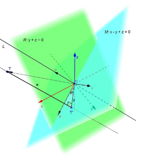
Figure 2: Cylindrical coordinates (r, $\theta,\,a)$ of $\boldsymbol{\boldsymbol{T}}=a\cdot\boldsymbol{\alpha}+b\cdot\boldsymbol{\beta}+c\cdot\boldsymbol{\boldsymbol{\gamma}}$ with respect to $L$ and $M$

4 Some Elementary Functions in $\mathbb{\mathbf{\mathbb{R}}}^{3}$

In what follows we are going to demonstrate the use of $J_{3}$-numbers as arguments of higher-order polynomials and some elementary functions, in particular the exponential function.

4.1 Polynomials of $J_{3}$-numbers and power series

Since the $\circledast$-multiplication of $J_{3}$-numbers is a closed operation in $\mathbb{\mathbf{\mathbb{R}}}^{3}$, one can recursively define the integer powers of a $J_{3}$-number as follows:

$$\boldsymbol{X}^{n}=\boldsymbol{X}^{n-1}\circledast\boldsymbol{X},\>\boldsymbol{X}^{0}=\boldsymbol{1},\>\boldsymbol{X}^{1}=\boldsymbol{X},\;n=1,2,...\$$

and consider polynomials in higher powers with coefficients $\boldsymbol{A}_{k}$ being $J_{3}$-numbers like it was done before for the quadratic in Subsection 1.10:

$$P(\boldsymbol{X})=\sum_{k=0}^{n}\boldsymbol{A}_{k}\circledast\boldsymbol{X}^{k}.\$$

Obviously, all the familiar algebraic manipulations with the real or complex polynomials remain unchanged for polynomials in $\mathbb{\mathbf{\mathbb{R}}}^{3}$. Similarly to the classical case we could also introduce formal infinite power series:

$$s(\boldsymbol{X})=\sum_{k=0}^{\infty}\boldsymbol{A}_{k}\circledast\boldsymbol{X}^{k},\;\boldsymbol{X}\in\mathbb{\mathbf{\mathbb{R}}}^{3}.\$$

4.2 $J_{3}$-trigonometric functions

Let us remind that the classical trigonometric functions $sin$ and $cos$ have the following power series representation

$$cos(x)=\sum_{n=0}^{\infty}\frac{(-1)^{n}x^{2n}}{(2n)!},\;sin(x)=\sum_{n=0}^{\infty}\frac{(-1)^{n}x^{2n+1}}{(2n+1)!}.\$$

Motivated by Euler’s formula that gives a connection between complex numbers, exponents and trigonometry

$$e^{\mathbf{i}x}=cos\,x+\mathbf{i}\,sin\,x,\;x\in\mathbb{\mathbf{\mathbb{R}}}\$$

we define three $J_{3}$-trigonometric functions of a real variable $x$:

$$cos_{0}(x)=\sum_{n=0}^{\infty}\frac{(-1)^{n}x^{3n}}{(3n)!},\ sin_{1}(x)=\sum_{n=0}^{\infty}\frac{(-1)^{n}x^{3n+1}}{(3n+1)!},\ sin_{2}(x)=\sum_{n=0}^{\infty}\frac{(-1)^{n}x^{3n+2}}{(3n+2)!}.\$$

It is easy to see that these power series are uniformly convergent and that $cos_{0},\,sin_{1}$, and $sin_{2}$ are all smooth functions that satisfy the following differential equations:

$$\frac{d}{dx}sin_{2}(x)=sin_{1}(x),\,\frac{d}{dx}sin_{1}(x)=cos_{0}(x),\,\frac{d}{dx}cos_{0}(x)=-sin_{2}(x).\$$

Moreover, similarly to the classical $sin$ and $cos$ functions that are solutions of a simple harmonic oscillator equation $y^{\prime\prime}(x)+y(x)=0$ each of the three $J_{3}$-trigonometric functions satisfy the following third order linear differential equation:

$$y^{\prime\prime\prime}(x)+y(x)=0.\$$

By solving (4.8) and taking into account (4.7) the $J_{3}$-trigonometric functions (4.6) can be expressed in terms of the standard elementary functions as follows:

$$\begin{array}[]{c}cos_{0}(x)=\frac{1}{3}e^{-x}(1+e^{\frac{3}{2}x}cos(\frac{\sqrt{3}}{2}x)),\\ \\ sin_{1}(x)=\frac{1}{3}e^{-x}(-1+e^{\frac{3}{2}x}(cos(\frac{\sqrt{3}}{2}x)+\sqrt{3}sin(\frac{\sqrt{3}}{2}x))),\\ \\ sin_{2}(x)=\frac{1}{3}e^{-x}(1-e^{\frac{3}{2}x}(cos(\frac{\sqrt{3}}{2}x)+\sqrt{3}sin(\frac{\sqrt{3}}{2}x))).\end{array}\$$

4.3 Exponential form of a $J_{3}$-number and Euler’s identity in $\mathbb{\mathbf{\mathbb{R}}}^{3}$

Definition 4.1. The exponent of a $J_{3}$-number $\boldsymbol{X}$ is defined as follows:

$$Exp(\boldsymbol{X})=\sum_{k=0}^{\infty}\frac{\boldsymbol{X}^{k}}{k!},\;\boldsymbol{X}\in\mathbb{\mathbf{\mathbb{R}}}^{3}.\$$

Due to the isomorphism (2.4) between $J_{3}$-numbers and Toeplitz matrices of the form (2.3) the above series converges absolutely and, moreover, in view of the commutativity:

$$Exp(\boldsymbol{X}+\boldsymbol{Y})=Exp(\boldsymbol{X})\circledast Exp(\boldsymbol{Y}),\;\forall\boldsymbol{X},\,\forall\boldsymbol{Y}\in\mathbb{\mathbf{\mathbb{R}}}^{3}.\$$

Remark. Note that $Exp(\boldsymbol{0})=\boldsymbol{1}$ and that $Exp(\boldsymbol{X})$ is always $\circledast$-invertible with the inverse

$$Exp(\boldsymbol{X}){}^{-1}=Exp(-\boldsymbol{X}),\;\forall\boldsymbol{X}\in\mathbb{\mathbf{\mathbb{R}}}^{3}.\$$

By inserting $\boldsymbol{X}=u+\boldsymbol{j}v+\boldsymbol{j}\boldsymbol{j}w$ into (4.10) and using (4.11) one could get the following factorization:

$$Exp(u+\boldsymbol{j}v+\boldsymbol{j}\boldsymbol{j}w)=Exp(u)\circledast Exp(\boldsymbol{j}v)\circledast Exp(\boldsymbol{j}\boldsymbol{j}w),\$$

where the first factor $Exp(u)=e^{u}$ is real while the remaining factors could be expressed due to $\boldsymbol{j}^{3}=-\boldsymbol{1}$ as follows:

$$Exp(\boldsymbol{j}\,v)=\sum_{k=0}^{\infty}\frac{(\boldsymbol{j}v)^{k}}{k!}=cos_{0}(v)+\boldsymbol{j}\,sin_{1}(v)+\boldsymbol{j}\boldsymbol{j}\,sin_{2}(v),\$$

$$Exp(\boldsymbol{j}\boldsymbol{j}\,w)=\sum_{k=0}^{\infty}\frac{(\boldsymbol{j}\boldsymbol{j}w)^{k}}{k!}=cos_{0}(-w)-\boldsymbol{j}\,sin_{2}(-w)-\boldsymbol{j}\boldsymbol{j}\,sin_{1}(-w).\$$

By combining (4.13)-(4.15) one gets

$$Exp(u+\boldsymbol{j}v+\boldsymbol{j}\boldsymbol{j}w)=f(u,v,w)+\boldsymbol{j}\,g(u,v,w)+\boldsymbol{j}\boldsymbol{j}\,h(u,v,w),\$$

where $f,\,g,\,h$ are as follows:

$$f=e^{u}(cos_{0}(v)\cdot cos_{0}(-w)+sin_{1}(v)\cdot sin_{1}(-w)+sin_{2}(v)\cdot sin_{2}(-w)),\$$

$$g=e^{u}(sin_{1}(v)\cdot cos_{0}(-w)+sin_{2}(v)\cdot sin_{1}(-w)-cos_{0}(v)\cdot sin_{2}(-w)),\$$

$$h=e^{u}(sin_{2}(v)\cdot cos_{0}(-w)+sin_{1}(v)\cdot sin_{2}(-w)-cos_{0}(v)\cdot sin_{1}(-w)).\$$

If one writes down $f,\,g,\,h$ in terms of standard elementary functions by (4.9) then the following outstanding formula would emerge after simplifications:

$$\begin{array}[]{cc}Exp(u+\boldsymbol{j}v+\boldsymbol{j}\boldsymbol{j}w)=&\frac{1}{3}e^{u-v+w}((1+2e^{3\varphi}\cos\theta)\ \ \ \ \ \ \,\ \ +\\ &\boldsymbol{j}(-1+e^{3\varphi}(\cos\theta+\sqrt{3}\sin\theta))\ \ \ +\\ &\boldsymbol{j}\boldsymbol{j}(1-e^{3\varphi}(\cos\theta-\sqrt{3}\cos\theta))\end{array}\$$

where $\varphi=\frac{1}{2}(v-w),\,\theta=\frac{\sqrt{3}}{2}(v+w)$.

In order to verify the above formula let us express:

$$\boldsymbol{X}=u+\boldsymbol{j}v+\boldsymbol{j}\boldsymbol{j}wi=s\cdot\boldsymbol{\alpha}+t\cdot\boldsymbol{\beta}+\theta\cdot\boldsymbol{\boldsymbol{\gamma}},\$$

where the orthogonal basis $\{\boldsymbol{\boldsymbol{\alpha}},\,\boldsymbol{\boldsymbol{\beta}},\,\boldsymbol{\boldsymbol{\boldsymbol{\gamma}}}\}$ is as in Subsection 1.8 and the coefficients $s,\,t,\,\theta$ are given by (1.41):

$$s=u-v+w,\,t=\frac{1}{2}(2u+v-w),\,\theta=\frac{\sqrt{3}}{2}(v+w).\$$

Lemma 11. For any real numbers $s$ and $t$ the following identity holds true:

$$Exp(s\,\boldsymbol{\alpha})\circledast Exp(t\,\boldsymbol{\beta})=e^{s}\boldsymbol{\alpha}+e^{t}\boldsymbol{\beta}.\$$

Proof.

By using $\boldsymbol{\alpha}+\boldsymbol{\beta}=\boldsymbol{1}$ and the idempotent property of $\boldsymbol{\alpha}$ and $\boldsymbol{\beta}$ let us evaluate each factor separately:

$$Exp(s\,\boldsymbol{\alpha})=\boldsymbol{1}+\sum_{n=1}^{\infty}\frac{(s\boldsymbol{\alpha})^{n}}{n!}=\boldsymbol{\alpha}+\boldsymbol{\beta}+\boldsymbol{\alpha}\cdot\sum_{n=1}^{\infty}\frac{s^{n}}{n!}=\boldsymbol{\beta}+\boldsymbol{\alpha}+\boldsymbol{\alpha}(e^{s}-1)=e^{s}\boldsymbol{\alpha}+\boldsymbol{\beta},\$$

$$Exp(t\,\boldsymbol{\beta})=\boldsymbol{1}+\sum_{n=1}^{\infty}\frac{(t\boldsymbol{\beta})^{n}}{n!}=\boldsymbol{\alpha}+\boldsymbol{\beta}+\boldsymbol{\beta}\cdot\sum_{n=1}^{\infty}\frac{t^{n}}{n!}=\boldsymbol{\alpha}+\boldsymbol{\beta}+\boldsymbol{\beta}(e^{t}-1)=\boldsymbol{\alpha}+e^{t}\boldsymbol{\beta},\$$

Finally, due to the $\circledast$-orthogonality of $\boldsymbol{\alpha}$ and $\boldsymbol{\beta}$ one can see:

$$Exp(s\,\boldsymbol{\alpha})\circledast Exp(t\,\boldsymbol{\beta})=(e^{s}\boldsymbol{\alpha}+\boldsymbol{\beta})\circledast(\boldsymbol{\alpha}+e^{t}\boldsymbol{\beta})=e^{s}\boldsymbol{\alpha}+e^{t}\boldsymbol{\beta},\$$

which completes the proof.□

Note that in view of (4.11) the above lemma immediately implies:

$$Exp(s\,\boldsymbol{\alpha}+t\,\boldsymbol{\beta})=e^{s}\boldsymbol{\alpha}+e^{t}\boldsymbol{\beta}.\$$

Lemma 12. For any real number $\theta$ the following identity holds true:

$$Exp(\theta\,\boldsymbol{\boldsymbol{\gamma}})=\boldsymbol{\alpha}+cos\,(\theta)\,\boldsymbol{\beta}+sin\,(\theta)\,\boldsymbol{\boldsymbol{\gamma}}.\$$

Proof.

By invoking (1.40) it is easy to check that $\boldsymbol{\boldsymbol{\gamma}}^{2k}=(-1)^{k}\!\boldsymbol{\beta}$ and $\boldsymbol{\boldsymbol{\gamma}}^{2k+1}=(-1)^{k}\boldsymbol{\beta}\circledast\!\boldsymbol{\boldsymbol{\gamma}}=(-1)^{k}\boldsymbol{\boldsymbol{\gamma}},\,k=1,2,..$ Thus

$$Exp(\theta\boldsymbol{\boldsymbol{\gamma}})=\sum_{n=0}^{\infty}\frac{(\theta\boldsymbol{\boldsymbol{\gamma}})^{n}}{n!}=\boldsymbol{1}+\sum_{k=2}^{\infty}\frac{(\theta\boldsymbol{\boldsymbol{\gamma}})^{2k}}{(2k)!}+\sum_{k=0}^{\infty}\frac{(\theta\boldsymbol{\boldsymbol{\gamma}})^{2k+1}}{(2k+1)!}$$

$$=\boldsymbol{\alpha}+(\boldsymbol{\beta}+\boldsymbol{\beta}\sum_{k=2}^{\infty}\frac{(-1)^{k}\theta{}^{2k}}{(2k)!})+\boldsymbol{\boldsymbol{\gamma}}\sum_{k=0}^{\infty}\frac{(-1)^{k}\theta{}^{2k+1}}{(2k+1)!}\$$

$$=\boldsymbol{\alpha}+cos\,(\theta)\,\boldsymbol{\beta}+sin\,(\theta)\,\boldsymbol{\boldsymbol{\gamma}}.\text{{\char 32\relax}}$$

Remark 1. One can regard (4.25) as the 3D analogue of the famous Euler’s formula $e^{i\varphi}=cos\,\varphi+\mathbf{i}\,sin\,\varphi$.

Theorem 4.1. For any real numbers $s,t,\,p$ the following identity holds true:

$$Exp(s\boldsymbol{\alpha}+t\boldsymbol{\beta}+\theta\boldsymbol{\boldsymbol{\gamma}})=e^{s}(\boldsymbol{\alpha}+e^{t-s}cos\,(\theta)\,\boldsymbol{\beta}+e^{t-s}sin\,(\theta)\,\boldsymbol{\boldsymbol{\gamma}}).\$$

Proof. It is enough to invoke (4.11) and apply Lemmas 11 and 12:

$$Exp(s\boldsymbol{\alpha}+t\boldsymbol{\beta}+\theta\boldsymbol{\boldsymbol{\gamma}})=Exp(s\boldsymbol{\alpha}+t\boldsymbol{\beta})\circledast Exp(\theta\boldsymbol{\boldsymbol{\gamma}})=e^{s}\boldsymbol{\alpha}+e^{t}cos\,(\theta)\,\boldsymbol{\beta}+e^{t}sin\,(\theta)\,\boldsymbol{\boldsymbol{\gamma}},$$

where the multiplication Table 2 has to be used.□

Remark 2. Let us note that (4.27) resembles the important classical formula $e^{x+iy}=e^{x}(cos\,y+\mathbf{i}\,sin\,y).$

Theorem 4.2. (Exponential form of a $J_{3}$-number).

If $\boldsymbol{\boldsymbol{S}}=a\cdot\boldsymbol{\alpha}+b\cdot\boldsymbol{\beta}+c\cdot\boldsymbol{\boldsymbol{\gamma}}$ is $\circledast$-invertible, then it admits the following representation:

$$\boldsymbol{\boldsymbol{S}}=(a\boldsymbol{\alpha}+r\boldsymbol{\beta})\circledast Exp(\theta\boldsymbol{\boldsymbol{\gamma}}),\>\$$

where $r=\sqrt{b^{2}+c^{2}}$ and $\theta=arctan(\frac{b}{c}$) if $c\neq 0$, or $\theta=arccot(\frac{c}{b}$) if $b\neq 0$.

Proof.

Since $\boldsymbol{\boldsymbol{S}}$ is $\circledast$-invertible at least one of coefficients $b$ or $c$ is nonzero, and hence one can define $\theta$. Furthermore, due to (3.18) one has:

$$\boldsymbol{\boldsymbol{S}}=(a\boldsymbol{\alpha}+r\boldsymbol{\beta})\circledast(\boldsymbol{\alpha}+cos(\theta)\boldsymbol{\beta}+sin(\theta)\boldsymbol{\boldsymbol{\gamma}}).\$$

It is enough now to combine (4.25) and (4.29).□

When plugging $\theta=2\pi k$ into (4.25) one gets the following formula:

$$Exp(2\pi k\boldsymbol{\boldsymbol{\gamma}})=\boldsymbol{1},\,k\in\mathbb{Z}\$$

which resembles the famous Euler’s identity: $e^{\mathbf{i}(\pi+2\pi k)}=-1,\,k\in\mathbb{Z}\text{.}$

Remark 3. There is no $J_{3}$-number $\boldsymbol{X}$ such that $Exp(\boldsymbol{X})=\boldsymbol{-1}$. This follows from the fact that according to (4.27) the altitude $|||Exp(\boldsymbol{X})|||=e^{s}>0$ while $|||\boldsymbol{-1}|||=-1$.

Theorem 4.3. The exponential curve $Exp(\theta\boldsymbol{\boldsymbol{\gamma}}),\>\theta\in\mathbb{R},$ is a circle in $\mathbb{\mathbf{\mathbb{R}}}^{3}$.

Proof. Let us observe that all the points of the curve $Exp(\theta\,\boldsymbol{\boldsymbol{\gamma}})=\boldsymbol{\alpha}+cos\,\theta\,\boldsymbol{\beta}+sin\,\theta\,\boldsymbol{\boldsymbol{\gamma}}$ are at the unit distance from both the origin $\boldsymbol{O}=(0,0,0)$  as well as from the $J_{3}$-invariant plane $M$. Indeed, it follows from (1.43) and (1.60) that for $\forall\theta\in\mathbb{R}$:

$$|Exp(\theta\boldsymbol{\boldsymbol{\gamma}})|=\sqrt{\frac{1^{2}+2cos^{2}\theta+2sin^{2}\theta}{3}}=1,\quad|||Exp(\theta\boldsymbol{\boldsymbol{\gamma}})|||=1.\$$

The unit altitude (see Remark 2 after Definition 7 of Subsection 1.10) means that all the points $Exp(\theta\boldsymbol{\boldsymbol{\gamma}})$ belong to the plane $x-y+z=1$ which is perpendicular to the axis L and intersects it at $\boldsymbol{\alpha}=\frac{1}{3}(1,-1,1)$. This plane intersects the unit sphere along a circle centered at $\boldsymbol{\alpha}$ with radius

$$\boldsymbol{r}=\sqrt{1-|\boldsymbol{\alpha}|^{2}}=\sqrt{1-\left(\frac{\sqrt{3}}{3}\right)^{2}}=\sqrt{\frac{2}{3}}=\frac{\sqrt{6}}{3},\$$

(see also Fig. 3 below). The rest is plain.□

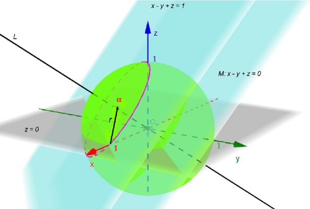
Figure 3: The exponential circle (in magenta) centered at $\boldsymbol{\alpha}$ with radius $\boldsymbol{r}$.

Finally, in order to verify formula (4.17) it is enough now to calculate the right hand side of (4.27) according to (4.19) and (1.42) :

$$Exp(u+\boldsymbol{j}v+\boldsymbol{j}\boldsymbol{j}w)=\frac{a+2b}{3}+\boldsymbol{j}\frac{-a+b+c\cdot\sqrt{3}}{3}+\boldsymbol{j}\boldsymbol{j}\frac{a-b+c\cdot\sqrt{3}}{3},\$$

where $a=e^{u-v+w},\,b=e^{\frac{1}{2}(2u+v-w)}cos(\frac{\sqrt{3}}{2}(v+w)),\,c=e^{\frac{1}{2}(2u+v-w)}sin(\frac{\sqrt{3}}{2}(v+w)).$

4.4 Logarithm of a $J_{3}$-number

The exponentiation of a $J_{3}$-number yields a $J_{3}$-number and thus is a closed operation.

It follows from (4.27) that for any $J_{3}$-number $\boldsymbol{X}=s\boldsymbol{\alpha}+t\boldsymbol{\beta}+\theta\boldsymbol{\boldsymbol{\gamma}}\,$ both the altitude of $Exp(\boldsymbol{X})$:

$$|||Exp(\boldsymbol{X})|||=e^{|||\boldsymbol{X}|||}=e^{s}>0,\$$

as well as the modulus of its projection on the plane $M$ are positive:

$$|e^{t}cos\,(\theta)\,\boldsymbol{\beta}+e^{t}sin\,(\theta)\,\boldsymbol{\boldsymbol{\gamma}}|=e^{t}>0.\$$

This means that the exponential function in $\mathbb{\mathbf{\mathbb{R}}}^{3}$ sends any $J_{3}$-number to $\mathbb{\mathbf{\mathbb{R}}}_{+}^{3}=\left\{\boldsymbol{X}=x+\boldsymbol{j}y+\boldsymbol{j}\boldsymbol{j}z:\>x-y+z>0,\>\boldsymbol{X}\notin L\right\}$ - the half-space which is above the $\boldsymbol{j}$-invariant plane $M$, with an exclusion of the $\boldsymbol{j}$-invariant line $L$. One could introduce the logarithm function on this domain $\mathbb{\mathbf{\mathbb{R}}}_{+}^{3}$ much in the same way as in the complex plane, namely, as an inverse to the exponential function $Exp.$

Definition 4.2. Given a $J_{3}$-number $\boldsymbol{Y}\in\mathbb{\mathbf{\mathbb{R}}}_{+}^{3}$, a $J_{3}$-number $\boldsymbol{X}$ is called the logarithm of $\boldsymbol{Y}$ (denoted by $\boldsymbol{X}=Log(\boldsymbol{Y})$) if $\boldsymbol{Y}=exp(\boldsymbol{X})$.

The $Log$ function in $\mathbb{\mathbf{\mathbb{R}}}^{3}$ is multivalued similarly to the classical logarithm in the complex plane. For example, due to (4.30) one has $Log(\boldsymbol{1})=\boldsymbol{0}+2\pi k\boldsymbol{\boldsymbol{\gamma}},\,k\in\mathbb{Z}.$

It follows from (4.11) that the $Log$ function is subject to the following logarithmic identity, up to $2\pi k\boldsymbol{\boldsymbol{\gamma}}$ for some $k\in\mathbb{Z}$:

$$Log(\boldsymbol{X}\circledast\boldsymbol{Y})=Log(\boldsymbol{X})+Log(\boldsymbol{Y}),\>\forall\boldsymbol{X},\,\boldsymbol{Y}\in\mathbb{\mathbf{\mathbb{R}}}_{+}^{3}\$$

If $\boldsymbol{X}\in\mathbb{\mathbf{\mathbb{R}}}_{+}^{3}$ and $n\in\mathbb{N}$ then (4.35) implies:

$$Log(\boldsymbol{X}^{n})=n\cdot Log(\boldsymbol{X})\$$

Since $|||\boldsymbol{j}|||=0-1+0=-1,\>Log(j)$ is not defined. Let us compute now $Log(\boldsymbol{j}^{2})$ instead. It is easy to see that $|\boldsymbol{j}^{2}|=1$ and $|||\boldsymbol{j}^{2}|||=1$, i.e., a point in $\mathbb{\mathbf{\mathbb{R}}}^{3}$, which corresponds to the $J_{3}$-number $\boldsymbol{j}\boldsymbol{j}$, belongs to the circle (4.29), and thus $Log(\boldsymbol{j}^{2})=\theta\boldsymbol{\boldsymbol{\gamma}}$ for some $\theta\in\mathbb{R}$. Since by (1.41)

$$\boldsymbol{j}^{2}=0+0\boldsymbol{j}+\boldsymbol{j}\boldsymbol{j}=\boldsymbol{\alpha}-\frac{1}{2}\boldsymbol{\beta}+\frac{\sqrt{3}}{2}\boldsymbol{\boldsymbol{\gamma}}\$$

it follows from (4.29) that $cos\,\theta=-\frac{1}{2},\>sin\,\theta=\frac{\sqrt{3}}{2}$. By solving this elementary trigonometric system one gets

$$Log(\boldsymbol{j}^{2})=\frac{2\pi}{3}\boldsymbol{\boldsymbol{\gamma}}+2\pi k\boldsymbol{\boldsymbol{\gamma}},\,k\in\mathbb{Z\ }$$

Finally, since by the basic property (1.2) $-\boldsymbol{j}=\boldsymbol{j}^{2}\circledast\boldsymbol{j}^{2}$ it is easy to compute: $Log(-\boldsymbol{j})=Log(\boldsymbol{j}^{2}\circledast\boldsymbol{j}^{2})=Log(\boldsymbol{j}^{2})+Log(\boldsymbol{j}^{2})=(\frac{4\pi}{3}+2\pi k)\boldsymbol{\boldsymbol{\gamma}}$, or

$$Log(-\boldsymbol{j})=(\frac{\pi}{3}+\pi(2k+1))\boldsymbol{\boldsymbol{\gamma}},\,k\in\mathbb{Z\ }$$

Epilogue

The three-dimensional hypercomplex $J_{3}$-number has been introduced. It is a scalar composed of three components which represents a point in $\mathbb{\mathbf{\mathbb{R}}}^{3},$ similarly to the complex number representing a point in the complex plane. The algebraic and geometric properties of $J_{3}$-numbers have been presented.

The analytic properties are out of the scope of the current work. We just note that $J_{3}$-analytic $\mathbb{\mathbf{\mathbb{R}}}^{3}$-valued function $F(z)=f(u,v,w)+\boldsymbol{j}\,g(u,v,w)+\boldsymbol{j}\boldsymbol{j}\,h(u,v,w)$ of a $J_{3}$-argument $z=u+\boldsymbol{j}v+\boldsymbol{j}\boldsymbol{j}w$ could be defined for which the analogue of the classical Cauchy - Riemann equations holds true:

$$\frac{\partial f}{\partial u}=\frac{\partial g}{\partial v}=\frac{\partial h}{\partial w},\ \frac{\partial g}{\partial u}=\frac{\partial h}{\partial v}=-\frac{\partial f}{\partial w},\ \frac{\partial h}{\partial u}=-\frac{\partial f}{\partial v}=-\frac{\partial g}{\partial w}.$$

Being a scalar, the $J_{3}$-numbers possess all attributes we demand from a scalar to have, that is being associative, commutative and distributive under addition as well as under multiplication. The reality that $J_{3}$-numbers are scalars enable their use as arguments in elementary functions as has been demonstrated.

The beauty of having a number, not a vector, representing a point in a 3D space is enchanting.

Bibliography

W. R. Hamilton, On the geometrical interpretation of some results obtained by calculation with biquaternions, Proceedings of the Royal Irish Academy, vol. 5, pp. 388–90, 1853.

B. L. van der Waerden, Modern Algebra, F. Ungar, New York; 3rd Edition, 1950.

B. L. van der Waerden, A History of Algebra: from al-Khwarizmi to Emmy Noether, Springer-Verlag, Berlin, 1985.

G. E. Hay, Vector and tensor analysis, Dover Publications, 1953.

Ruel V. Churchill, Complex Variables and Applications, McGraw-Hill Inc., US; 2nd edition, December 1960.

E. Dale Martin, A system of three-dimensional complex variables, NASA technical report, 1986.

I. Kantor and A. Solodovnikov, Hypercomplex numbers, Springer-Verlag, New York, 1989.

P. Kelly, R. L Panton, and E Dale Martin, Three-dimensional potential flows from functions of a 3D complex variable, Fluid Dynamics Research 6:119-137, 1990.

G. B. Price, An Introduction to Multicomplex Spaces and Functions, Marcel Dekker, New York, 1991.

G.Turk and M. Levoy, Zippered Polygon Meshes from Range Images, in Computer Graphics Proceedings, ACM SIGGRAPH, pp. 311-318, 1994.

C. M. Davenport, A commutative hypercomplex algebra with associated function theory, in Clifford Algebras With Numeric and Symbolic Computations, pp 213-227, 1996.

S. Olariu, Complex numbers in three dimensions, arXiv:math.CV/0008120, 2000.

S. Olariu, Complex numbers in N dimensions, Elsevier, 2002.

Jian-Jun Shu, and Li Shan Ouw, Pairwise alignment of the DNA sequence using hypercomplex number representation, Bulletin of Mathematical Biology, Vol. 66, No. 5, pp. 1423-1438, 2004.

Wolfram Research, Inc., Mathematica, Version 5.1, Champaign, IL, 2004.

Alfsmann, D., Gockler, H.G., Sangwine, S.J., Ell, T.A., Hypercomplex algebras in digital signal processing: Benefits and drawbacks. In: Proc. 15th European Signal Processing Conference, pp. 1322–1326, 2007

Anderson, M., Katz V.J., and Wilson R.J. Who Gave You the Epsilon?: And Other Tales of Mathematical History. Washington, DC: Mathematical Association of America, 2009.

GeoGebra. Version 5.0. URL http://http://www.geogebra.org/, 2014.

R Core Team. R: A language and environment for statistical computing. Version 3.2.1, R Foundation for Statistical Computing, Vienna, Austria. URL http://www.R-project.org/, 2015.

Daniel Adler, Duncan Murdoch and others. rgl: 3D Visualization Using OpenGL. R package version 0.95.1260/r1260. http://R-Forge.R-project.org/projects/rgl/, 2015.

Ya. O. Kalinovsky, Yu. E. Boyarinova, I. V. Khitsko, Reversible Digital Filters Total Parametric Sensitivity Optimization using Non-canonical Hypercomplex Number System, arXiv:cs.NA/1506.01701, 2015.

Michael Shmoish

Afterword

The story of a quest for a proper three-dimensional analogue of the complex numbers is rich and fascinating. You probably remember the famous question Hamilton’s sons used to ask him every morning in early October 1843: "Well, Papa, can you multiply triples?" Sir W. R. Hamilton, according to his own letter, was always obliged to reply, with a sad shake of the head: "No, I can only add and subtract them." Soon after he saw a way to multiply quadruples leading to his prominent discovery of quaternions.

I first met Mr. Shlomo Jacobi under sad circumstances in early 2012, when he had just lost his beloved wife to a deadly disease. Still Shlomo was strong enough to talk about his idea of three-dimensional hypercomplex numbers and to show me the following ingenious multiplication of triples

$$\begin{matrix}(a,\,b,\,c)\circledast\,(u,\,v,\,w)=&(au-bw-cv,\,av+bu-cw,\,aw+bv+cu),\end{matrix}$$

that he discovered in early 1960s, shortly before his graduation from the Technion.

It was extremely important to Hamilton that the modulus of a product of two vectors would be equal to the product of their moduli. This law of moduli requirement (which is impossible to achieve in dimension three due to the well-known theorems by Frobenius and Hurwitz on real division algebras) was abandoned by Shlomo in favor of commutativity of the above $\boldsymbol{\circledast}$-product even though zero divisors appeared. "They only add interest" as Olga Taussky Todd put it once. Previous attempts to introduce hypercomplex numbers were mostly algebraic, Hamilton and his successors were trying to devise a "wise" multiplication table. The above article suggests a purely geometric approach by defining a linear operator $\boldsymbol{j}$ which transforms the three-dimensional Euclidean space into itself:

$$\boldsymbol{j}:\,(x,\,y,\,z)\rightarrow(-z,\,x,\,y)$$

and thus mimics the multiplicative action of imaginary unit in the complex plane: $\,\mathbf{i}\cdot\,(x+\mathbf{i}y)=(-y+\mathbf{i}x)$. The $\circledast$-product emerges naturally from the basic properties of operator $\boldsymbol{j}$ and a definition of three-component $\boldsymbol{J_{3}}$-numbers, while the law of moduli happens to be replaced by moduli inequality:

$$|\boldsymbol{\boldsymbol{S}}\circledast\mathit{\boldsymbol{\boldsymbol{T}}}|\leq\sqrt{3}\cdot|\boldsymbol{\boldsymbol{S}}|\,|\mathit{\boldsymbol{\boldsymbol{T}}}|.$$

Though Shlomo’s article is mainly concerned with geometric and algebraic aspects of the $J_{3}$-numbers, many analytic properties of complex numbers and complex-valued functions could be extended properly to the three-dimensional case due to the above inequality.

After the discovery of quaternions some generalizations of the classical complex numbers to higher (usually >= 4) dimensions were developed, such as matrices, general hypercomplex number systems, and Clifford geometric algebras. As for dimension three, I would mention an article by Silviu Olariu where the geometric, algebraic, and analytical properties of his tricomplex numbers, the close relatives of Shlomo’s $J_{3}$-numbers, were studied in detail. Note that Shlomo was unaware of Olariu’s works as well as earlier NASA reports by E. Dale Martin (on the theory of three-component numbers and their applications to potential flows) listed in the above bibliography section. I’ve compiled this short bibliography which provides only a limited overview of hypercomplex-related field and contains several mathematical textbooks from Shlomo’s bookshelf.

Shlomo’s main idea was that $J_{3}$-numbers are scalars that could be dealt with conveniently once accustomed. Algebra $\mathbb{\mathbf{\mathbb{R}}}_{\circledast}^{3}$ of $J_{3}$-numbers is linked to geometry in three dimensions in a simple and natural way. Based on Shlomo’s mostly elementary article, the advanced notions of invariant subspaces, idempotents, structured matrices, algebra isomorphism could be explained easily to undergraduate students via visualization in 3D space. The commutativity and useful analytical properties hopefully makes the $J_{3}$-numbers a valuable addition to the current toolbox of rotation matrices and quaternions for manipulating objects in 3D space, optimal tracking and robotic applications. There is also some evidence that the hypercomplex systems similar to $J_{3}$-numbers prove useful in cryptography, physics, digital signal processing, alignment of DNA sequences, and study of the 3D structure of macromolecules.

The representation of entire $\mathbb{\mathbf{\mathbb{R}}}^{3}$ as the $\circledast$-product of a half-plane and a circle according to formula (3.20) might be advantageous. In particular, one can decompose any three-dimensional body like the Stanford bunny (in blue) into the planar part (in cyan) and the arc (in green) and then manipulate (e.g., cluster or encrypt) each component separately. The $\boldsymbol{\circledast}$-product would give then a fast and easy way to recover the modified 3D object.

The "bunny" illustration has been produced using R-package ’rgl’ and my R-script based on the original Shlomo’s code written in Wolfram Mathematica, while all the figures in the above article have been produced by myself using the 3D GeoGebra.

I hope that this article will serve as a tribute to a dear friend Shlomo Jacobi and to his life-long passion for mathematics.