Transition radiation at radio frequencies from ultra-high energy neutrino-induced showers

Abstract

Coherent radiation at radio frequencies from high-energy showers fully contained in a dense radio-transparent medium - like ice, salt, soil or regolith - has been extensively investigated as a promising technique to search for ultra-high energy (UHE) neutrinos. Additional emission in the form of transition radiation may occur when a neutrino-induced shower produced close to the Earth surface emerges from the ground into atmospheric air. We present the first detailed evaluation of transition radiation from high-energy showers crossing the boundary between two different media. We found that transition radiation is sizable over a wide solid angle and coherent up to $\sim$ 1 GHz. These properties encourage further work to evaluate the potential of a large-aperture UHE neutrino experiment based on detection of transition radiation.

I Introduction

The nature and origin of UHE cosmic rays (UHECRs) with energies around $10^{20}$ eV is one of the most puzzling questions in particle astrophysics Nagano and Watson (2000); Watson (2014). Charged cosmic rays with energy less than $\sim$ 10 EeV are significantly scattered by the galactic magnetic field and cannot be traced back to their origin. At higher energies where deflections become less important, the cosmic ray flux falls steeply Abraham et al. (2010); Fukushima (2015), requiring giant experiments like the Pierre Auger Observatory Aab et al. (2015) and the Telescope Array Abu-Zayyad et al. (2012) to collect reasonable statistics. Neutrinos, which travel undeflected through the universe, may provide important clues on the origin of UHECRs Kotera and Olinto (2011). In fact, cosmic rays interacting with matter and radiation present at the accelerating source, or encountered along their path towards Earth, may produce UHE neutrinos. Recently, extraterrestrial neutrinos of energies up to few PeV have been detected by the IceCube Neutrino Observatory Aartsen et al. (2013). For neutrino energies in the EeV range, a promising detection technique is based on the radio signal from the neutrino-induced shower in a dense radio-transparent medium. Ice has been proven to be an ideal medium for this technique by pioneering experiments such as RICE Kravchenko et al. (2003), which buried radio antennas in the South Pole ice, and ANITA Gorham et al. (2009), which looks with balloon-flown radio antennas over a large portion of the Antarctica ice cap. Large ground arrays of antennas, buried in ice (ARA Allison et al. (2012)) or on the ice surface (ARIANNA Barwick et al. (2015) and GNO Wissel et al. (2015)) are now under development. In another interesting approach, several groups James et al. (2010); Gorham et al. (2004); Beresnyak et al. (2005) have pointed radiotelescopes towards the Moon, searching for radiopulses from neutrino interactions in the lunar regolith. All of these experiments are based on the Askaryan effect Askar’yan (1962) - the emission of coherent Cherenkov radiation from the $\sim 20\%$ excess of electrons present in an electromagnetic shower.

In this paper we explore transition radiation (TR) Ginzburg and Frank (1945) at radio frequencies as a possible way to detect UHE neutrinos. Transition radiation is emitted by charged particles when crossing the boundary between two media with different indices of refraction. From the theoretical viewpoint, TR can be understood as the radiation required to match at the boundary the electric field produced by the charged particle in the bulk of the two media. It has been well studied both theoretically and experimentally; for a comprehensive review of transition radiation, see for example Ter-Mikaelian (1972). However, there are only a few estimates in the literature of TR from cosmic ray showers - either crossing from atmospheric air to a denser medium (e.g. clouds Gazazian et al. (2001) or ground de Vries et al. (2015)) or emerging from ground into air (a rough estimate is given in Falcke et al. (2004)). While the methods presented in this paper are of general application, we are mostly motivated by the study of TR emitted when a shower, originated by a UHE neutrino interaction below the Earth surface, escapes the ground into the atmosphere. In fact, the net electric charge corresponding to the excess electrons of the shower will produce an upward-going transition radiation when passing through the ground - atmosphere boundary. Since showers in dense media are rather compact in size, we expect the TR to be coherent up to GHz frequencies, with significant advantages in the cost of detectors and background noise level. In this work we present the first detailed evaluation of transition radiation from high-energy showers crossing the boundary between two different media.

In Section II, we present a general method to calculate transition radiation from a shower crossing the boundary between two media using the far-field limit. This method extends the well-known Zas-Halzen-Stanev (ZHS) algorithm Zas et al. (1992) to account for boundary matching of the radiation field. In ZHS, the trajectory of each particle in a homogeneous medium is approximated by linear segments, sufficiently small that the particle can be assumed to move uniformly, and the corresponding electromagnetic radiation is computed exactly in the Fraunhofer limit from the Maxwell equations Zas et al. (1992). In the extended ZHS algorithm, hereafter called ZHS-TR, a particle segment crossing the two media is split at the boundary James et al. (2011) and reflection and refraction of the radiation emitted by the two track segments is then included in a standard way Ginzburg and Tsytovich (1990).

In Section III, the properties of TR emitted by a high energy shower when crossing from a dense medium to air are studied in detail. In particular, we investigate the spectral characteristics of the TR signal and their dependence on the shower energy and zenith angle, on the stage of the shower development at the boundary, on the energy of the shower particles, and on the type of dense medium.

Conclusions are drawn in Section IV.

II Transition radiation from high-energy showers: calculations

II.1 The ZHS Monte Carlo

Our calculation of radio emission from particle showers crossing the boundary between two media is based on the methods Allan (1971); Zas et al. (1992); Garcia-Fernandez et al. (2013) implemented in the ZHS Monte Carlo, which simulates electromagnetic showers and their associated coherent radio emission up to EeV energies Alvarez-Muniz et al. (2009). Originally developed for the Fraunhofer limit in homogeneous ice Halzen et al. (1991), it has been extended to other dielectric homogeneous media Alvarez-Muniz et al. (2009, 2006) and to reproduce near field effects by dividing the particle trajectories in sufficiently small sub-tracks Alvarez-Muniz et al. (2000). To provide the reader with the necessary background, the methods currently implemented in the ZHS Monte Carlo are reviewed in the following.

The ZHS Monte Carlo follows electrons and positrons interactions down to a kinetic energy threshold of 100 keV. Charged particles below this threshold contribute negligibly to the electric field, which is proportional to the particle tracklength Zas et al. (1992). The simulation includes bremsstrahlung, pair production, and the interactions responsible for the generation of the excess charge (Møller, Bhabha, Compton scattering and electron-positron annihilation). In addition, multiple elastic scattering (according to Molière’s theory) and continuous ionization losses are implemented. The track segment between two consecutive particle interactions is divided into multiple linear segments, along which the particle is assumed to move with constant velocity. To ensure a proper calculation in the Fraunhofer limit, the maximum equivalent depth of each sub-track does not exceed 0.1 radiation lengths. Also, for low energy particles the size of the sub-track is required to be smaller than the particle range, and this step size is used to evaluate ionization losses and multiple elastic scattering. Accurate bookkeeping of the absolute timing is maintained during particle propagation, including geometrical time delays as well as those introduced by different particle velocities (a uniform energy loss along the sub-track is assumed for this purpose). An approximate account is also made of the time delay induced by multiple elastic scattering. From the position and time of the endpoints of the sub-tracks, the frequency spectrum of the electric field is derived. The total electric field at the observer’s location is then calculated by superposition of the electric field from each sub-track, with relative phase shifts due to different starting point positions and time delays properly taken into account.

The electric field $\boldsymbol{E}(t,\boldsymbol{x})$ produced by a charged particle moving with uniform velocity $\boldsymbol{v}$ between two fixed points in a homogeneous medium can be derived from Maxwell equations, and has a frequency Fourier transform

$$\boldsymbol{E}(\omega,\boldsymbol{x})=2\int_{-\infty}^{\infty}\boldsymbol{E}(t,\boldsymbol{x})e^{i\omega t}dt$$ (1)

given by Zas et al. (1992):

$$\boldsymbol{E}(\omega,\boldsymbol{x})=\frac{e\mu_{r}}{2\pi\epsilon_{0}c^{2}}i\omega\frac{e^{ikR}}{R}e^{i(\omega-\boldsymbol{k}\cdot\boldsymbol{v})t_{1}}\boldsymbol{v}_{\perp}\left[\frac{e^{i(\omega-\boldsymbol{k}\cdot\boldsymbol{v})\delta t}-1}{i(\omega-\boldsymbol{k}\cdot\boldsymbol{v})}\right].$$ (2)

In Eq. (2), $R$ is the distance from the track to the observer, which is assumed to be large enough for the Fraunhofer regime to be valid. Wave vector $\boldsymbol{k}$ points in the direction from the track to the observer and has modulus ${k}=\omega/c^{\prime}$, with $c^{\prime}$ the speed of light in the medium. Also, ${\boldsymbol{v}}_{\perp}=-\hat{\boldsymbol{k}}\times(\hat{\boldsymbol{k}}\times\boldsymbol{v})$ is the component of $\boldsymbol{v}$ in the plane perpendicular to the unit vector $\hat{\boldsymbol{k}}=\boldsymbol{k}/|\boldsymbol{k}|$. Finally, $t_{1}$ and $t_{2}=t_{1}+\delta t$ are the absolute times at which the particle passes through the starting point and endpoint of the sub-track, respectively. In magnetic materials, $\mu_{r}$ is the relative permeability of the medium.

II.2 The ZHS-TR algorithm

II.2.1 General case: Transition between two media

The original ZHS Monte Carlo described in Sect. II.1 has been mostly used in simulations where the shower is contained in a single dense medium, which also hosts the observer. Several modifications are required to simulate a shower extending over two different media. In the following, we will detail the ZHS-TR algorithm for a shower starting in a medium of refractive index $n_{1}$, separated by a planar boundary from a second medium of refractive index $n_{2}$ where the observer is located. This configuration accounts for the case of a shower initiated below the Earth surface by an UHE neutrino interaction, and emerging in the atmosphere where it is detected. However, the algorithm is general and can be used for other cases (for example, the shower could start in air, or the observer could be located in medium 1).

As in the original ZHS algorithm, a particle track is approximated by linear segments along which the particle is assumed to move with constant velocity. However, the electric field from a given sub-track can include one, two or three contributions, depending on whether the sub-track is fully contained in medium 1, in medium 2 (where the observer is) or crossing the boundary. The different contributions are pictorially represented in Fig. 1. We calculate the electric field at the observer position, with the sub-track viewed in the direction $\hat{\boldsymbol{k}}$. Also, we assume that Fraunhofer conditions apply, namely $\lambda R\gg D^{2}$ and $R\gg D$, where $\lambda$ is the wavelength of the radiation and $D$ the characteristic size of the sub-track. With this approximation the factor $1/R$ in Eq. (2) can be factored out as if it was constant.

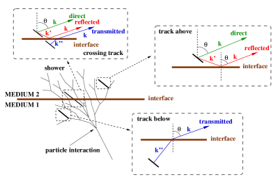
Figure 1: Schematic illustration of the ZHS-TR algorithm (see text for a detailed description). The three cases shown correspond to a sub-track crossing the interface, a sub-track in the same medium as the observer (track above) and a sub-track in the other medium (track below).

For tracks fully contained in medium 1, the only contribution comes from the electric field (Eq. (2)) emitted into direction $\hat{\boldsymbol{k}^{\prime\prime}}$ (the direction of a ray refracted at the boundary into direction $\hat{\boldsymbol{k}}$ according to Snell’s law, see Fig. 1). The radiated electric field is then decomposed into $s$ and $p$ polarizations (perpendicular and parallel to the plane of incidence, respectively), and transmitted through the boundary applying the appropriate Fresnel coefficients Jackson (1999). Because we are dealing with a point source and not plane waves, the standard transmission Fresnel coefficients must be multiplied by a factor

$$\frac{n_{2}}{n_{1}}\frac{\cos\theta}{\sqrt{1-\left[\frac{n_{2}}{n_{1}}\sin\theta\right]^{2}}},$$ (3)

which can be understood as describing the change in divergence of rays upon transmission James et al. (2011). The angle of refraction $\theta$ is the angle between the unit vector $\hat{\boldsymbol{k}}$ and the normal to the boundary plane. The final transmission formulas read

$$t_{p} = \frac{2n_{2}\cos\theta}{n_{2}\sqrt{1-\left[\frac{n_{2}}{n_{1}}\sin\theta\right]^{2}}+n_{1}\cos\theta},$$

$$t_{s} = \frac{2n_{2}\cos\theta}{n_{1}\sqrt{1-\left[\frac{n_{2}}{n_{1}}\sin\theta\right]^{2}}+n_{2}\cos\theta}.$$ (4)

When calculating the electric field at the observer position, the $p$ polarization in the reflection plane remains of course perpendicular to $\hat{\bf k}$, the new propagation direction after refraction. In the following we refer to the electric field corresponding to tracks fully contained in medium 1 as the “transmitted contribution”.

For tracks fully contained in medium 2, two distinct contributions must be evaluated. The first is the standard contribution given by Eq. (2) describing the electric field radiated into direction $\hat{\boldsymbol{k}}$ (“direct contribution”). The second contribution (“reflected contribution”) comes from radiation emitted into a direction $\hat{\boldsymbol{k}}^{\prime}$ which is reflected off the boundary into the observing direction $\hat{\boldsymbol{k}}$ (Fig. 1). Eq. (2) is also used to calculate this contribution. The electric field is again decomposed into $s$ and $p$ polarizations, and the appropriate Fresnel coefficients are used for reflection:

$$r_{p} = \frac{n_{1}\cos\theta-n_{2}\sqrt{1-\left[\frac{n_{2}}{n_{1}}\sin\theta\right]^{2}}}{n_{1}\cos\theta+n_{2}\sqrt{1-\left[\frac{n_{2}}{n_{1}}\sin\theta\right]^{2}}},$$

$$r_{s} = \frac{n_{2}\cos\theta-n_{1}\sqrt{1-\left[\frac{n_{2}}{n_{1}}\sin\theta\right]^{2}}}{n_{2}\cos\theta+n_{1}\sqrt{1-\left[\frac{n_{2}}{n_{1}}\sin\theta\right]^{2}}}.$$ (5)

Since reflection does not change the divergence of rays, Eqs. (II.2.1) have their usual plane-wave form. As in the transmitted contribution, the $p$ polarization remains perpendicular to $\hat{\bf k}$ after reflection.

Finally, for tracks crossing the two media the following procedure is applied. The track is split at the boundary plane into two sub-tracks, as in James et al. (2011). Each sub-track is then fully contained in one medium and the methods previously described can be applied to calculate the electric field. For these tracks transition radiation is naturally accounted for with this procedure. In the ZHS algorithm each of the endpoints of a sub-track contributes a term to the electric field. For a charged particle moving uniformly in a homogeneous medium (i.e. with constant velocity along the track), the contributions from the common endpoints of two adjacent sub-tracks cancel exactly. Thus, the electric field associated to the track does not depend on the number or on the length of its sub-tracks. On the other hand, a track crossing two media has two adjacent sub-tracks with common endpoints located at the boundary. Since these endpoints are associated to sub-tracks contained in media with different index of refraction, their contributions do not cancel exactly. Transition radiation appears because of this incomplete cancellation. Notice that the assumption of uniform velocity can be made to an arbitrary degree of precision by reducing the length of the sub-tracks.

The electric field produced by the entire shower is then obtained from the superposition of the individual contributions of all particle tracks. Explicit geometric phase differences between tracks on both sides of the boundary plane are appropriately taken into account in this procedure. This concludes the ZHS-TR algorithm.

The technical implementation of the ZHS-TR algorithm requires two simulation runs, since the original ZHS code was developed for a single homogeneous medium. The simulation starts by generating and propagating the shower in medium 1. Then, particles crossing the boundary are propagated in medium 2 in a separate simulation. The ZHS code presents some limitations, since it does not treat hadronic interactions and radio emission induced by the Earth magnetic field Huege and Falcke (2003), and assumes a constant density of the media, which is not appropriate for atmospheric air. However, neglecting these effects should not impact significantly our results as discussed in Sect. III.

II.2.2 Vacuum approximation

In the case under consideration, transition radiation is produced when the shower exits into the atmosphere. Since the air density is much lower than the density of the medium where the shower originated, medium 2 can be reasonably approximated by vacuum to simplify calculations. There is no difference in the simulation for the portion of the shower contained in medium 1: particle tracks are treated as in Sect. II.2.1, and their corresponding transmitted contribution is calculated. Instead, particles crossing the boundary, which do not interact in vacuum, are modeled as moving to infinity with constant velocity. The electric field associated to such a semi-infinite track James et al. (2011) in the Fraunhofer regime is given by:

$$\boldsymbol{E}(\omega,\boldsymbol{x})=-\frac{e\mu_{r}}{2\pi\epsilon_{0}c^{2}}i\omega\frac{e^{ikR}}{R}\frac{\boldsymbol{v}_{\perp}e^{i(\omega-\boldsymbol{k}\cdot\boldsymbol{v})t_{1}}}{i(\omega-\boldsymbol{k}\cdot\boldsymbol{v})},$$ (6)

where the notation follows Eq. (2). The origin of this formula can be understood by dividing the semi-infinite track into sub-tracks. The electric field is obtained by summing Eq. (2) over all sub-tracks. Since contributions of the common endpoints of adjacent sub-tracks cancel, the only term left corresponds to the starting point (the term at infinity goes as $1/R\rightarrow 0$), thus giving Eq. (6).

Notice that since the electric field of the entire track is given by Eq. (6), there is no need for a division in sub-tracks, which makes the simulation faster. Equation (6) is then used to calculate the direct and reflected contributions to the electric field following the procedure of Sect. II.2.1. We will apply the vacuum approximation in Sect. III.1.2.

II.3 Transition radiation from a single particle

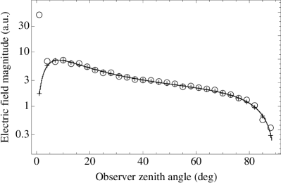
Figure 2: Angular distribution of the far-field electric field radiated by a single charged particle crossing from ice to air: comparison of the results obtained using the ZHS-TR algorithm with sub-tracks 10 cm (crosses) and 100 cm (open dots) long to the exact calculation (black line).

A basic check of the ZHS-TR algorithm was performed by estimating the transition radiation from a single charged particle and comparing the result with the classical derivation Ginzburg and Tsytovich (1990). An electron crossing the boundary from ice to air in the vertical direction was considered for this purpose. The electron velocity was fixed to $0.99c$, corresponding to an energy of about 3.6 MeV. In order to approximate an infinite track (required for the classical derivation), electron interactions were not considered, and a total track length of 100 km was equally divided between the two media. We then evaluated the electric field at an observer position $\bf d$ of zenith angle $\theta$, and $|{\bf d}|=1$ km (the origin of the coordinate system coincides with the intersection of the track with the boundary plane). Since this distance is much larger than the length of the sub-tracks in ZHS-TR, we expect the Fraunhofer limit used in Eq. (2) to be a good approximation.

In Fig. 2, the electric field calculated with our algorithm is compared with the exact result obtained by solving the Maxwell equations for an infinite track Ginzburg and Tsytovich (1990). The two approaches are in practically perfect agreement when sub-tracks of 10 cm length are used in ZHS-TR. To illustrate the importance of the Fraunhofer limit, we also show the same comparison for sub-tracks of 100 cm length. At small zenith angles, where a discrepancy is observed, the perpendicular distance between the track and the observer ($\sim|{\bf d}|\theta$) becomes comparable to the length of the sub-tracks, and the Fraunhofer regime is no longer valid.

In the rest of the paper, we will assume that the observer is always distant enough from the shower for the Fraunhofer regime to be valid. Due to the finite extent of the shower, this is a good approximation in most practical cases, for example in the detection of the TR signal from a satellite or balloon instrument Gorham et al. (2009), Motloch et al. (2014).

III Properties of transition radiation from high-energy showers

In this section, we investigate in detail the properties of the radiation emitted by an electromagnetic shower transitioning from a dense medium to air. Showers initiated by a 100 TeV electron in ice ($n_{1}=1.78$ at radio frequencies) were used in most of these studies. Also, no thinning was employed in the simulation of the showers (i.e. all particles were propagated). Since in the Fraunhofer approximation the electric field ${\mathbb{E}}(\omega,{\bf x})$ is inversely proportional to the distance $R$ to the shower, results are presented in terms of the quantity $|R\times{\mathbb{E}}|$. The case of a vertical shower is treated first, and then results for inclined showers - which may be more realistic for a UHE neutrino-induced interaction - are presented.

III.1 Vertical showers

III.1.1 Direct, reflected and transmitted contributions

The angular distribution of the electric field radiated by a 100 TeV vertical shower simulated with ZHS-TR is shown in Fig. 3 (black solid line). The shower’s starting point in ice was chosen appropriately for the shower maximum to occur approximately at the ice–air boundary. The zenith angle dependence reflects the contributions to TR by single electrons whose angular features are shown in Fig. 2. The weak angular dependence of the emitted radiation is a notable feature, when compared to coherent Cherenkov radiation which is strongly beamed around the Cherenkov angle Zas et al. (1992). A value of $|R\times{\mathbb{E}}|\sim 5\times 10^{-7}\,\mathrm{V/MHz}$ is obtained for this shower.

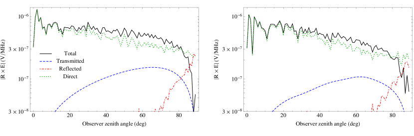
Figure 3: Angular distribution of the electric field radiated by a single 100 TeV vertical shower crossing from ice to air: scaled magnitudes of the total field (black), direct (green short dashes), reflected (red dot-dashes) and transmitted (blue dashes) contributions. Due to phase differences the total magnitude can be smaller than those of individual parts. See the text for details. The electric field is evaluated at 200 MHz (left panel) and 1 GHz (right panel).

Figure 4: Ratio of the electric field magnitudes calculated in the vacuum approximation and the full simulation (solid) and the same comparison for simulation where we include only tracks crossing the ice–air boundary (dashed). The vertical shower started with 100 TeV energy and crossed from ice to air. The electric field is evaluated at 200 MHz (left panel) and 1 GHz (right panel).

Also shown in Fig. 3 are the contributions to the total electric field (direct, transmitted and reflected) introduced in Sect. II.2.1. The direct contribution from particle tracks in air is dominant at all angles, and presents a peak at $\sim 2^{\circ}$. This peak can be understood as Cherenkov radiation produced in air (Cherenkov angle $\sim 1.4^{\circ}$) by the high energy shower particles which follow closely the shower axis. In addition, there are noticeable fluctuations around the mean value of $|R\times{\bf E}|$, which are due to the fine structure of the shower development in air. In fact, the spatial dimension corresponding to the frequencies of observation - 200 MHz and 1 GHz - is much smaller than the transverse size of the shower (a simulation performed at 10 MHz, not shown for the sake of brevity, presents a much smoother behavior). The reflected contribution is negligible except for the largest angles, where it becomes comparable to the direct contribution. However, the two contributions cancel each other for an observer looking orthogonally to the shower axis, since a $\pi$ phase shift is gained upon reflection, and the total electric field drops at zenith angles approaching $90^{\circ}$. Lastly, the transmitted contribution from particles in ice is never dominant for a vertical shower. In fact, the coherent Cherenkov radiation from the Askaryan effect in ice undergoes total internal reflection at the ice–air boundary plane (the Cherenkov angle is larger that the critical angle for $n_{1}$=1.78) and cannot reach the observer. However, this component can become significant for inclined showers, see Sect. III.2.

III.1.2 Particles crossing the boundary and vacuum approximation

To further investigate the origin of the emitted radiation, we performed a dedicated ZHS-TR simulation where the electric field was calculated taking into account only contributions from particles crossing the ice – air boundary. Results are shown in Fig. 4, where we plot the ratio of the electric field magnitudes obtained in this simplied simulation and the electric field magnitudes of the full result. Indeed, transition radiation from particles crossing the boundary accounts for most of the emission (at low zenith angles, Cherenkov radiation from particles propagating in air is dominant, as seen in Fig. 3).

Also shown in Fig. 4 is a ratio of the electric field magnitudes resulting from a ZHS-TR simulation using the vacuum approximation of Sect. II.2.2 with the electric field magnitudes of the full result. The vacuum approximation reproduces the full ZHS-TR simulation reasonably well, with a notable exception at low zenith angles. This can be explained by the fact that, for an observer looking from the vertical direction, highly relativistic particles with $\boldsymbol{k}\parallel\boldsymbol{v}$ have $\omega-\boldsymbol{v}\cdot\boldsymbol{k}\sim 0$, resulting in a large contribution from Eq. (6). High energy particles emerge from ice strongly beamed along the vertical axis, and since their direction does not change in the vacuum approximation, a strong peak is expected. On the other hand, the full ZHS-TR simulation includes particle interactions in air which randomize the directions of the sub-tracks, leading to a suppression of the peak. In any case, the agreement between the vacuum approximation and the full simulation over most of the zenith angles suggests that the details of the shower development in air have a marginal effect on the TR emission. Thus, we expect that neglecting the altitude dependence of the air density and geomagnetic effects in particle propagation will not change significantly our estimates of transition radiation.

III.1.3 Frequency spectrum

Another important property of the radiation is its frequency spectrum, shown in Fig. 5 for 100 TeV showers. To reduce shower-to-shower fluctuations, a hundred showers were simulated, and the modulus of their signal was averaged. All averages will be done this way unless explicitly stated. The rise at the highest frequencies is caused by contributions from incoherent emission and continues well beyond the frequencies displayed. To check that the coherent contribution is indeed quickly dying away after certain threshold frequency, we fitted a power law dependence to the magnitude of the electric field above 20 GHz where the coherent contributions are negligible. When we subtracted this contribution from the total electric field observed in the simulations, the remainder showed the expected steep drop off.

Unlike coherent Cherenkov radiation, which drops off at relatively low frequencies away from the Cherenkov angle Zas et al. (1992), transition radiation is coherent up to $\sim 1\,\mathrm{GHz}$ over a wide range of angles. The physical origin of this effect may be understood with a simplified model where TR is produced only by particles crossing orthogonally the boundary plane with velocity $c$, uniformly distributed over a disk of radius $r_{M}\sim$ 11 cm (the Molière radius in ice). Under these approximations, each particle contributes equally in amplitude, and only the relative phases due to propagation are important. The problem then becomes analogous to calculating the diffraction pattern of a uniformly-illuminated circular aperture Jackson (1999). Thus, the electric field at given frequency $f$ goes as

$$|{\bf E}|\sim\frac{c}{f\sin\theta}J_{1}\left(\frac{2\pi fr_{M}}{c}\sin\theta\right),$$ (7)

where $J_{1}$ is a Bessel function of the first kind. This expression is maximal for $f\rightarrow 0$ and reaches the first zero when

$$f\sim\frac{0.61c}{r_{M}\sin\theta}.$$ (8)

This equation may be taken as an estimate of the TR cutoff frequency. Indeed, the trend observed in Fig. 5, with lower cutoff frequencies corresponding to larger angles of observation, is well described qualitatively by Eq. (8).

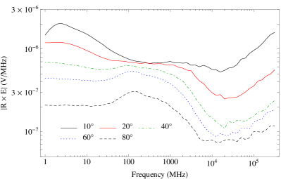
Figure 5: Frequency spectrum of the electric field radiated by a 100 TeV vertical shower crossing from ice to air, at $10^{\circ}$ (black solid), $20^{\circ}$ (red solid), $40^{\circ}$ (green dot dashes), $60^{\circ}$ (blue short dashes), and $80^{\circ}$ (black long dashes) zenith angle of observation (top to bottom). Each curve is an average of a hundred showers. The rise at the highest frequencies comes from incoherent emission.

III.1.4 Scaling with number of particles crossing the boundary

We have shown in Sect. III.1.2 that most of the emission from a shower emerging from ice into air is due to particles crossing the boundary. These particles should contribute coherently to the radio signal up to a cutoff frequency related to the geometrical size of the shower. Thus, we expect the averaged electric field $\langle R\times E\rangle$ to scale linearly with the charge excess $\Delta Q$ (the number of electrons minus the number of positrons) flowing through the boundary.

To test this we used an averaged value

$$\langle E\times R\rangle = \frac{1}{C}\int_{10^{\circ}<\theta<70^{\circ}}\left|R\times E(200\,\mathrm{MHz},\theta)\right|\mathrm{d}\Omega$$ (9)

$$= \frac{1}{C^{\prime}}\int_{10^{\circ}}^{70^{\circ}}\left|R\times E(200\,\mathrm{MHz},\theta)\right|\sin\theta\mathrm{d}\theta,$$

where the normalization constants are

$$C^{\prime}=\frac{C}{2\pi}=\int_{10^{\circ}}^{70^{\circ}}\sin\theta\mathrm{d}\theta.$$ (10)

This quantity measures an average magnitude of the electric field in the middle angular region which is not affected by the air Cherenkov emission or the decrease of the signal at large zenith angles.

The theoretically predicted linear scaling is confirmed in Fig. 6, which shows the dependence of the average magnitude of the electric field as a function of the charge excess for a hundred simulated 100 TeV showers starting at a fixed distance $500\,\mathrm{g/cm^{2}}$ from the ice-air boundary. One can notice the presence of showers with charge excess of only 60% of the maximum observed value. This effect is related to the fact that while for most of the showers $500\,\mathrm{g/cm^{2}}$ corresponds approximately to the distance to the shower maximum, for others the shower maximum occurs at a somewhat different distance. This affects the number of crossing particles and relatedly the size of the mean electric field.

On top of the systematic increase and decrease of the mean value of the electric field with the charge excess through the boundary there is also the effect of the fine structure of an individual shower. This leads to fluctuations around the mean value, seen for example in Fig. 3. From this figure we can estimate the magnitude of these fluctuations for a 100 TeV shower; for showers of higher energies these fluctuations are relatively smaller due to higher total number of particles in these showers.

In another related study, we simulated 100 TeV showers starting at different ice depths. Since the number of particles crossing the boundary depends in this case on the stage of the shower development, the signal should be largest when the maximum of the shower development occurs close to the boundary for a typical shower. This is indeed confirmed in Fig. 7. The peak at low observation angles ($<5^{\circ}$), which is due to Cherenkov radiation from particles in air, becomes less pronounced the farther the shower starting point is from the boundary. In fact, at later stages of the shower development the shower is less compact and its particles have a larger angular spread, resulting in a loss of coherence.

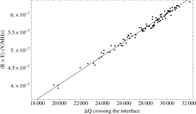
Figure 6: Relation between the absolute charge excess crossing the boundary and the averaged electric field for a hundred 100 TeV showers starting 500 g/cm² from the ice-air boundary. The straight line is a fit of the expected theoretical dependence.

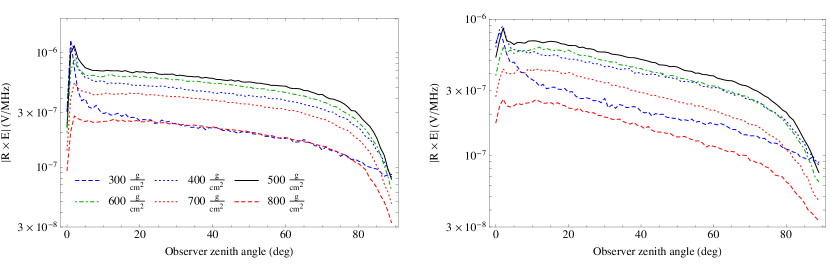
Figure 7: Angular distribution of the electric field radiated by a 100 TeV vertical shower crossing from ice to air, with starting point in ice at 300 (blue long dashes), 400 (blue short dashes), 500 (black, showers typically crossing at shower maximum), 600 (green dot-dashes), 700 (red short dashes) and 800 (red long dashes) $\mathrm{g/cm^{2}}$ from the ice–air boundary. The electric field is evaluated at 200 MHz (left panel) and 1 GHz (right panel). Each curve is an average of a hundred showers.

III.1.5 Dependence on shower particles energy spectrum

Since the electric field depends on the particle velocity (c.f. Eq. (2)), we may expect a dependence of the TR on the energy spectrum of the shower particles. To study this dependence, we estimated the electric field for 100 TeV simulated showers taking into account only the contributions of sub-tracks from particles with energy below a given threshold. Results are presented in Fig. 8 (note the linear scale of the vertical axis). The highest energy particles ($>100$ MeV) contribute mostly at low zenith angles. In fact, these particles are strongly beamed in the vertical direction, and account for the coherent Cherenkov peak as discussed in Sect. III.1.1. The contributions from particles in the energy ranges 3–10 MeV, 10–30 MeV, and 30–100 MeV are comparable. This is due to a compensation between the number of particles – which is higher at low energies – and the amount of radiation coming from a single particle – which is higher at high energies. Particles with energies below 3 MeV do not contribute significantly.

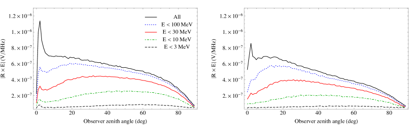
Figure 8: Angular distribution of the electric field radiated by a 100 TeV vertical shower crossing from ice to air (from top to bottom): all particles (black), particles with energy $<$100 MeV (blue short dashes), 30 MeV (red), 10 MeV (green dot dashes) and 3 MeV (black long dashes). The electric field is evaluated at 200 MHz (left panel) and 1 GHz (right panel). Each curve is an average of a hundred showers.

III.1.6 Dependence on the shower energy

We expect the absolute charge excess for showers which cross the boundary at their maximum developments to be a good proxy of the shower energy as the number of particles at the shower maximum is roughly proportional to the shower energy. As a consequence, we expect the electric field to scale linearly with the shower energy.

In our implementation of the ZHS-TR algorithm it is not possible to know a priori whether a given simulated shower will hit the boundary around the shower maximum or whether it will be one of the downward fluctuations seen in the Fig. 6. To quantitatively asses how the radiated electric field depends on the shower energy, we then compare maximal signal seen in all our simulated showers at three different energies: 1, 10 and 100 TeV. As a first step we run several trial showers to find for each of these energies an approximate starting point where we can expect showers reaching the boundary at roughly their shower maximum. We then simulate a hundred unthinned showers starting at this point and search for the maximal value of $\langle E\times R\rangle$. We take this quantity (denoted as $\langle E\times R\rangle^{\rm max}$ as our proxy for the value of $\langle E\times R\rangle$ for a shower hitting the boundary at the shower maximum. Similar other choices are possible but lead all to comparable results.

The maximal values of the mean electric field at these three energies observed in our sample of showers are

$$\langle E\times R\rangle^{\rm max}_{100\,\mathrm{TeV}} = 6.4\times 10^{-7}\,\mathrm{V/MHz}$$ (11)

$$\langle E\times R\rangle^{\rm max}_{10\,\mathrm{TeV}} = 7.8\times 10^{-8}\,\mathrm{V/MHz}$$

$$\langle E\times R\rangle^{\rm max}_{1\,\mathrm{TeV}} = 1.2\times 10^{-8}\,\mathrm{V/MHz}.$$

They deviate slightly from the theoretical prediction, which we attribute to higher effect of fluctuations at lower energies. This viewpoint is supported by Fig. 9, which shows the angular distributions of the electric fields averaged over the investigated showers. While the 100 TeV showers show profiles comparable to those of a single particle, at lower energies the fluctuations lead to a change in the shape of the profile. Notice that even for 100 TeV showers the agreement with the single particle profile is worse at higher frequencies due to the lower level of coherence.

As a further study, we investigated several thinned 1 EeV showers. After finding an approximate shower development $D$ to the shower maximum we then repeated the simulation for showers with starting point separated by distance $D$ from the interface. Due to increased computational demands we simulated only twelve showers for this energy. The largest value of $\langle E\times R\rangle$ we found among these showers is

$$\langle E\times R\rangle^{\rm max}_{1\,\mathrm{EeV}}=1.52\,\mathrm{mV/MHz}\approx 2400\,\langle E\times R\rangle^{\rm max}_{100\,\mathrm{TeV}}.$$ (12)

The reason why the electric field at very high energies does not scale linearly with the energy can be traced back to the Landau-Pomeranchuk-Migdal (LPM) effect Landau and Pomeranchuk (1953a, b). As was found in Alvarez-Muniz and Zas (1997), due to elongation of the shower at EeV and higher energies the number of particles around shower maximum for a shower with the LPM effect included decreases with respect to the same shower with no LPM effect. Consequently, the charge excess and the radiated electric field are also lowered.

Figure 9: Angular distribution of the electric field radiated by 1 (short dash), 10 (long dash) and 100 TeV (solid) vertical shower crossing from ice to air. The electric field is evaluated at 200 MHz (left panel) and 1 GHz (right panel). Each curve is an average of a hundred showers.

III.1.7 Different media

So far, we have studied the properties of TR from showers crossing an ice–air interface. Salt, soil and regolith are also potentially relevant for an experiment, and we performed simulations of 100 TeV showers starting in these media. For soil we took parameters of the soil from the Argentinian village El Sosneado, next to the Pierre Auger Observatory location. The angular distribution of the electric field radiated in salt/regolith/soil simulations is compared with the standard ice simulation in Fig. 10. At 200 MHz, the electric field is comparable for all four media. At 1 GHz, a lower emission is obtained in ice. This can be explained by the larger Molière radius of this medium ($\sim$ roughly double of the other $r_{M}$), which results in a less compact shower. Since the condition of coherent emission from the shower particles is then more easily broken, a weaker electric field is expected. Soil and lunar regolith have rather similar behaviors at both frequencies.

To illustrate an additional feature which can occur for certain configurations, we performed a simulation, also shown in Fig. 10, in which the refractive index of a medium, otherwise similar to ice, was artificially set to value of 1.28 so that the Cherenkov angle is smaller than the critical angle for total internal reflection in this medium (see Sect.III.1.1) and the coherent Askaryan radiation produced by the shower in the artificial ice is now transmitted into air (see Sect.III.1.1). Notice that the refracted Cherenkov radiation is significantly larger than the TR, and presents a characteristic angular distribution, with a beam clearly visible at 1 GHz where coherence effects are stronger. A signal of similar origin will be encountered in the study of inclined showers in Sect. III.2.

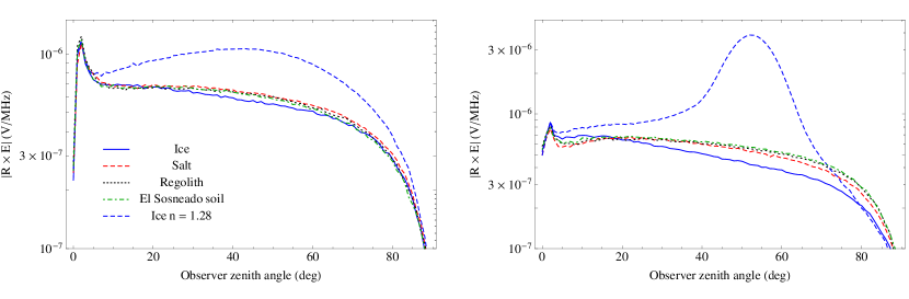
Figure 10: Angular distribution of the electric field radiated by a 100 TeV vertical shower crossing from ice (blue), salt (red dashes), regolith (black short dashes) and soil at El Sosneado (green dot-dashes) to air. Also shown is the electric field for a simulation where the ice refractive index was set to the unphysical value of 1.28 (blue long dashes). The electric field is evaluated at 200 MHz (left panel) and 1 GHz (right panel). Each curve is an average of a hundred showers.

III.2 Inclined showers

While some specific applications of transition radiation from close-to-vertical showers may be found (for example, showers emerging from a mountain range), a more likely use of TR could be the detection of UHE neutrinos through inclined showers emerging from the Earth surface. In fact, the Earth becomes increasingly opaque for neutrino energies above 100 TeV Gandhi et al. (1998), and most of the observable showers would originate from Earth-skimming neutrinos interacting below the Earth surface.

To gain insight on the properties of TR from inclined showers, we performed simulations of 100 TeV showers with large zenith angle crossing the boundary from ice to air. The shower’s starting point in ice was chosen so that the shower maximum development would occur at the intersection of the shower axis and the boundary plane. Results of the simulations for two showers with incident angles of $\theta_{\rm sh}=45^{\circ}$ and $75^{\circ}$, respectively, are first shown in Figs. 12 and 12. In these graphs, each point corresponds to the electric field in a direction $(\theta,\phi)$ of observation, the polar angle of the plot being equal to $\phi$ and its radial distance from the origin proportional to $\theta$. Due to symmetry of the situation, we show only half of the sky in each plot. The direction of the shower axis $(\theta_{\rm sh},\phi_{\rm sh}=0^{\circ})$ is marked by a cross. The electric field was evaluated at 50 and 1 GHz. In Figs. 14 and 14 we show the electric field for the same physical situation evaluated along lines of constant $\phi$ for $\phi=0^{\circ},30^{\circ},60^{\circ}$ and $90^{\circ}$; profiles along $\phi$ and $\phi+180^{\circ}$ are plotted using a single curve with the latter corresponding to negative values of $\theta$. Each curve is an average over a hundred showers.

Several distinctive features characterize the radiation. At 50 MHz, the electric field is sizable over a large portion of the hemisphere even for the $75^{\circ}$ shower, with an intensity comparable to that of a vertical shower. Also, there is a small angular region around the direction of the shower axis where the electric field increases by a factor of about three, clearly visible in Fig. 14 and 14. This peak corresponds to Cherenkov emission in air by high energy shower particles moving close to the shower axis (see left panel of Fig. 8). As also evident in Figs. 14 and 14, the electric field drops significantly for $(\theta,\phi)=(\theta_{\rm sh},\phi_{\rm sh})$ due to vanishing $\boldsymbol{v}_{\perp}$ in Eq. (2) for $\boldsymbol{v}\parallel\boldsymbol{k}$.

At 1 GHz, the emission is overall more beamed towards the direction of the shower axis, and this effect is more pronounced the higher the frequency and the incident angle of the shower. For the $75^{\circ}$ shower, $|R\times{\bf E}|$ is greater than $10^{-6.5}\,\mathrm{V/MHz}$ in $\sim 50\%$ of the hemisphere at 50 MHz, and only in $\sim 20\%$ of the hemisphere at 1 GHz. Another distinctive feature at high frequency is the appearance of an angular band with significantly increased signal. The band is clearly evident at 1 GHz, where the electric field is an order of magnitude larger. Its origin is explained in terms of coherent Cherenkov radiation refracted from ice into air. Indeed, we found that most of the radiation in this angular region is coming from below the boundary (“refracted contribution”). Further insight is given by a simple model where the Cherenkov cone produced by a highly relativistic particle moving in ice along the shower axis is refracted into air according to Snell’s law. The refracted Cherenkov cone matches very well the position and shape of the observed band, confirming its association to coherent Cherenkov emission by shower particles in ice.

At 10 MHz, the emitted radiation is basically indistinguishable for showers leaving either ice or soil when both are crossing the interface at their shower maximum. At higher frequencies both electric field profiles show rise of the Cherenkov peak and increased beaming towards the direction of the shower axis; these features start to appear at lower frequencies in ice for reasons explained in section III.1.7.

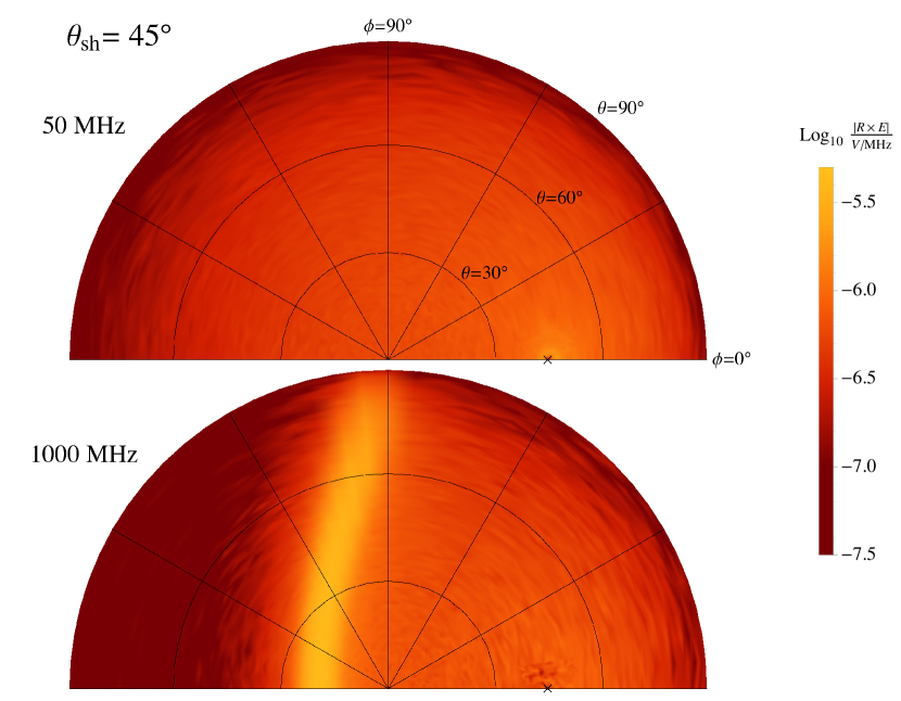
Figure 11: Angular distribution of the electric field radiated by a 100 TeV inclined shower crossing from ice to air with incident zenith angle of $\theta_{\rm sh}=45^{\circ}$ and $\phi_{\rm sh}=0^{\circ}$. Each point corresponds to the electric field in a direction $(\theta,\phi)$ of observation, the polar angle is equal to $\phi$ and the radial distance from the origin proportional to $\theta$. The shower leaves medium 1 (ice) into medium 2 (air) while crossing at shower maximum. Due to symmetry of the situation we show ony half of the sky in each plot. The direction of the shower axis is represented by a cross. The electric field is evaluated at a frequency of 50 MHz (top) and 1 GHz (bottom).

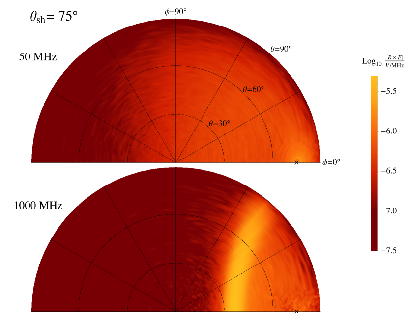
Figure 12: Same as Fig. 12 for a shower with incident zenith angle of $\theta_{\rm sh}=75^{\circ}$ and $\phi_{\rm sh}=0^{\circ}$.

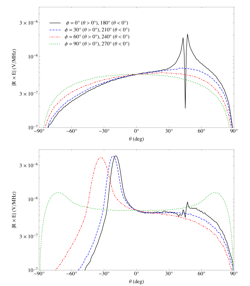
Figure 13: Angular distribution of the electric field radiated by a 100 TeV inclined shower crossing from ice to air with incident zenith angle of $\theta_{\rm sh}=45^{\circ}$ and $\phi_{\rm sh}=0^{\circ}$. Each curve corresponds to the shower profile with fixed observer position $\phi$ while varying $\theta$ (see caption of Fig. 12). Plotted for $\phi=0^{\circ},30^{\circ},60^{\circ}$ and $90^{\circ}$; profiles along $\phi$ and $\phi+180^{\circ}$ are plotted using a single curve with the latter corresponding to negative values of $\theta$. The shower leaves medium 1 (ice) into medium 2 (air) while crossing at shower maximum. The electric field is evaluated at a frequency of 50 MHz (top) and 1 GHz (bottom). Each curve is an average of a hundred showers.

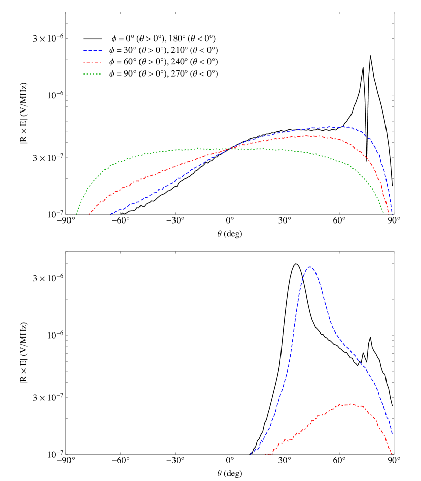
Figure 14: Same as Fig. 14 for a shower with incident zenith angle of $\theta_{\rm sh}=75^{\circ}$ and $\phi_{\rm sh}=0^{\circ}$.

IV Conclusions

We have developed a general method to calculate the electric field radiated by the ensemble of particles of a high-energy electromagnetic shower developing in two different media. The algorithm is based on the standard ZHS Monte Carlo approach, where a particle track is divided into sub-tracks, each contributing to the total electric field. In the special case of a particle crossing the two media, the particle track is split at the boundary, and the electric field from the two sub-tracks is evaluated taking properly into account reflection and refraction at the boundary plane. Transition radiation naturally arises from this procedure, in addition to the coherent Cherenkov radiation produced by the shower particles within each medium.

Our ZHS-TR algorithm has general applicability and could be used, for example, to evaluate the radiation from an Extensive Air Shower hitting ground, as seen by an observer placed above (or below) the Earth surface. In this paper, we focused our studies on the radiation emitted at radio frequencies by showers transitioning from a dense medium into air. This configuration is relevant for a shower originated by a UHE neutrino interaction below the Earth surface, escaping ground into the atmosphere. The ZHS Monte Carlo treats only electromagnetic showers, which are appropriate for a charged-current interaction of a high-energy electron neutrino. However, we expect our results not to change significantly for hadronic showers (produced in charged or neutral-current interactions of neutrinos of any flavor) since a large fraction of their energy is ultimately dissipated in electromagnetic processes Alvarez-Muniz and Zas (1998).

Fundamental properties of the radiation were determined through Monte Carlo simulations of vertical showers crossing from ice to air. We found that the emission is fairly isotropic, with an electric field strength of $\sim 5\times 10^{-11}$ V/MHz/m for a 100 TeV shower observed at 10 km distance. The electric field scales approximately linearly with the number of particles crossing the boundary and remains coherent up to $\sim 1$ GHz. At EeV energies the growth of the signal magnitude with shower energy is slower than linear, due to the LPM effect. Similar results were obtained when using salt, soil or regolith as a dense medium. We also studied the characteristics of radio emission from inclined showers. The radiation pattern is quite broad, but becomes more beamed towards the direction of the shower axis for larger incident angles or higher emission frequencies. The electric field strength is similar to that of a vertical shower, but increases significantly at frequencies of $\sim 1$ GHz in a limited angular band, corresponding to a coherent Cherenkov cone refracted from ice into air. Electric field for showers leaving soil show similar features, only their onset appears at higher frequencies due to better coherence in this medium.

Amongst these results, the angular distribution and frequency spectrum of the radiation are particularly interesting. Given the wide solid angle of the emission, a large aperture experiment becomes feasible. Also, substantial radiation in the GHz range facilitates detection, thanks to the low radio background and advantages in detector design at these frequencies. These observations encourage further studies to evaluate the potential of a large-aperture UHE neutrino experiment based on detection of transition radiation.

Acknowledgments.– The authors would like to dedicate this paper to Prof. Raymond Protheroe who sadly passed away in July 2015. Ray got JAM and EZ interested in this topic while visiting Santiago de Compostela in spring 2007 as part of his sabbatical leave. We also thank Justin Bray and Clancy James for discussions on this topic over the last years and Roland Crocker for early work. Finally, we would like to thank the anonymous referee for his many invaluable suggestions.

This work was supported in part by NSF grant PHY-1412261 and by the Kavli Institute for Cosmological Physics at the University of Chicago through grant NSF PHY-1125897 and an endowment from the Kavli Foundation and its founder Fred Kavli. JAM and EZ additionally thank Ministerio de Economía (FPA2012-39489), Consolider-Ingenio 2010 CPAN Programme (CSD2007-00042), Xunta de Galicia (GRC2013-024), Feder Funds and CESGA (Centro de Supercomputación de Galicia) for computing resources.

References

- Nagano and Watson (2000) M. Nagano and A. A. Watson, Rev. Mod. Phys. 72, 689 (2000).
- Watson (2014) A. A. Watson, Rept. Prog. Phys. 77, 036901 (2014), arXiv:1310.0325 [astro-ph.HE] .
- Abraham et al. (2010) J. Abraham et al. (Pierre Auger), Phys.Lett. B685, 239 (2010), arXiv:1002.1975 [astro-ph.HE] .
- Fukushima (2015) M. Fukushima (Telescope Array), (2015), arXiv:1503.06961 [astro-ph.HE] .
- Aab et al. (2015) A. Aab et al. (Pierre Auger), Submitted to: Nucl. Instrum. Meth. (2015), arXiv:1502.01323 [astro-ph.IM] .
- Abu-Zayyad et al. (2012) T. Abu-Zayyad et al. (Telescope Array), Nucl. Instrum. Meth. A689, 87 (2012), arXiv:1201.4964 [astro-ph.IM] .
- Kotera and Olinto (2011) K. Kotera and A. V. Olinto, Ann. Rev. Astron. Astrophys. 49, 119 (2011), arXiv:1101.4256 [astro-ph.HE] .
- Aartsen et al. (2013) M. Aartsen et al. (IceCube), Science 342, 1242856 (2013), arXiv:1311.5238 [astro-ph.HE] .
- Kravchenko et al. (2003) I. Kravchenko et al. (RICE), Astropart. Phys. 19, 15 (2003), arXiv:astro-ph/0112372 [astro-ph] .
- Gorham et al. (2009) P. W. Gorham et al. (ANITA), Astropart. Phys. 32, 10 (2009), arXiv:0812.1920 [astro-ph] .
- Allison et al. (2012) P. Allison et al., Astropart. Phys. 35, 457 (2012), arXiv:1105.2854 [astro-ph.IM] .
- Barwick et al. (2015) S. W. Barwick et al. (ARIANNA), Astropart. Phys. 70, 12 (2015), arXiv:1410.7352 [astro-ph.HE] .
- Wissel et al. (2015) S. A. Wissel et al., PoS(ICRC2015) , 1150 (2015).
- James et al. (2010) C. W. James, R. D. Ekers, J. Alvarez-Muniz, J. D. Bray, R. A. McFadden, C. J. Phillips, R. J. Protheroe, and P. Roberts, Phys. Rev. D81, 042003 (2010), arXiv:0911.3009 [astro-ph.HE] .
- Gorham et al. (2004) P. W. Gorham, C. L. Hebert, K. M. Liewer, C. J. Naudet, D. Saltzberg, and D. Williams, Phys. Rev. Lett. 93, 041101 (2004), arXiv:astro-ph/0310232 [astro-ph] .
- Beresnyak et al. (2005) A. R. Beresnyak, R. D. Dagkesamansky, A. V. Kovalenko, V. V. Oreshko, and I. M. Zheleznykh, Astron. Rep. 49, 127 (2005).
- Askar’yan (1962) G. Askar’yan, Sov.Phys.JETP 14, 441 (1962).
- Ginzburg and Frank (1945) V. Ginzburg and I. Frank, J.Phys.(USSR) 9, 353 (1945).
- Ter-Mikaelian (1972) M. L. Ter-Mikaelian, High energy electromagnetic processes in condensed media, Internat. Sci. Tracts Phys. Astron. (Wiley, New York, NY, 1972).
- Gazazian et al. (2001) E. D. Gazazian, K. Ispirian, and A. S. Vardanyan, AIP Conf. Proc. 597, 111 (2001).
- de Vries et al. (2015) K. D. de Vries, S. Buitink, N. van Eijndhoven, T. Meures, A. O’Murchadha, et al., (2015), arXiv:1503.02808 [astro-ph.HE] .
- Falcke et al. (2004) H. Falcke, P. Gorham, and R. J. Protheroe, International SKA Conference 2003 Geraldton, Australia, July 27-August 2, 2003, New Astron. Rev. 48, 1487 (2004), arXiv:astro-ph/0409229 [astro-ph] .
- Zas et al. (1992) E. Zas, F. Halzen, and T. Stanev, Phys.Rev. D45, 362 (1992).
- James et al. (2011) C. W. James, H. Falcke, T. Huege, and M. Ludwig, Phys.Rev. E84, 056602 (2011), arXiv:1007.4146 [physics.class-ph] .
- Ginzburg and Tsytovich (1990) V. L. Ginzburg and V. N. Tsytovich, Transition radiation and transition scattering. (Hilger, Bristol, UK, 1990).
- Allan (1971) H. Allan, Radio Emission from Extensive Air Showers (North-Holland, Amsterdam, 1971) pp. 169–302.
- Garcia-Fernandez et al. (2013) D. Garcia-Fernandez, J. Alvarez-Muniz, W. R. Carvalho, A. Romero-Wolf, and E. Zas, Phys.Rev. D87, 023003 (2013), arXiv:1210.1052 [astro-ph.HE] .
- Alvarez-Muniz et al. (2009) J. Alvarez-Muniz, C. James, R. Protheroe, and E. Zas, Astropart.Phys. 32, 100 (2009).
- Halzen et al. (1991) F. Halzen, E. Zas, and T. Stanev, Phys.Lett. B257, 432 (1991).
- Alvarez-Muniz et al. (2006) J. Alvarez-Muniz, E. Marques, R. A. Vazquez, and E. Zas, Phys.Rev. D74, 023007 (2006), arXiv:astro-ph/0512337 [astro-ph] .
- Alvarez-Muniz et al. (2000) J. Alvarez-Muniz, R. Vazquez, and E. Zas, Phys.Rev. D62, 063001 (2000), arXiv:astro-ph/0003315 [astro-ph] .
- Note (1) Note we use a non-standard convention.
- Jackson (1999) J. D. Jackson, Classical electrodynamics, 3rd ed. (Wiley, New York, NY, 1999).
- Huege and Falcke (2003) T. Huege and H. Falcke, Astron. Astrophys. 412, 19 (2003), arXiv:astro-ph/0309622 [astro-ph] .
- Motloch et al. (2014) P. Motloch, N. Hollon, and P. Privitera, Astropart.Phys. 54, 40 (2014), arXiv:1309.0561 [astro-ph.IM] .
- Landau and Pomeranchuk (1953a) L. D. Landau and I. Pomeranchuk, Dokl. Akad. Nauk Ser. Fiz. 92, 535 (1953a).
- Landau and Pomeranchuk (1953b) L. D. Landau and I. Pomeranchuk, Dokl. Akad. Nauk Ser. Fiz. 92, 735 (1953b).
- Alvarez-Muniz and Zas (1997) J. Alvarez-Muniz and E. Zas, Phys. Lett. B411, 218 (1997), arXiv:astro-ph/9706064 [astro-ph] .
- Gandhi et al. (1998) R. Gandhi, C. Quigg, M. H. Reno, and I. Sarcevic, Phys.Rev. D58, 093009 (1998), arXiv:hep-ph/9807264 [hep-ph] .
- Alvarez-Muniz and Zas (1998) J. Alvarez-Muniz and E. Zas, Phys. Lett. B434, 396 (1998), arXiv:astro-ph/9806098 [astro-ph] .