Optimum Traffic Allocation in Bundled Energy Efficient Ethernet Links

Abstract

The energy demands of Ethernet links have been an active focus of research in the recent years. This work has enabled a new generation of Energy Efficient Ethernet (EEE) interfaces able to adapt their power consumption to the actual traffic demands, thus yielding significant energy savings. With the energy consumption of single network connections being a solved problem, in this paper we focus on the energy demands of link aggregates that are commonly used to increase the capacity of a network connection. We build on known energy models of single EEE links to derive the energy demands of the whole aggregate as a function on how the traffic load is spread among its powered links. We then provide a practical method to share the load that minimizes overall energy consumption with controlled packet delay, and prove that it is valid for a wide range of EEE links. Finally, we validate our method with both synthetic and real traffic traces captured in Internet backbones.

I Introduction

Energy consumption is nowadays a global source of concern for both economic and environmental reasons. Networking equipment alone consumes 1.8% of the world’s electricity, and that number is currently increasing at a 10% rate annually [1]. If we just focus on data centers, between 15 and 20% of electricity is used for networking [2]. These reasons are spurring the development of more power efficient networking equipment.

A direct result of these efforts is the IEEE 802.3az standard [3] which provides a new idle mode for Ethernet physical interfaces. This new mode only needs a small fraction of the power used in normal operation, but no traffic can be transmitted nor received while the interface stays in the idle mode. Since there is an implicit trade-off between energy consumption and frame delay, these new Energy Efficient Ethernet (EEE) interfaces need a governor that decides when to enter and exit this idle mode. In fact, several alternatives have already been proposed in the literature [4, 5, 6, 7] and have been later validated by both empirical [8, 9] and analytic means [10, 11, 12, 13, 14]. These works have provided us with the tools needed to accurately estimate the power savings of EEE for any arrival traffic pattern with the more prevalent idle mode governors and to properly tune them to maximize energy savings.

With the energy consumption problem of single Ethernet links mostly solved we focus in this paper on the power demands of network connections formed by multiple EEE links, either by link aggregation [15] or some other proprietary means. Despite the existence of EEE for saving energy in the individual components of the bundle, the global consumption of an aggregate may be severely affected by how the incoming traffic is shared among its powered up links. In fact, the power profiles of the individual EEE links are not linear, as their energy demands do not grow proportionally to the offered load. This makes the overall power consumption dependent on the actual traffic share among the links of the aggregate.

The main goal of this paper is to obtain the optimum share of traffic among the links of an aggregate from an energy efficiency perspective. As far as we know, this is the first paper to tackle this issue. We propose a water-filling algorithm, where traffic is only transmitted on a given link if all the previous ones are already being used at their maximum capacity and show that it is optimum for various relevant traffic arrival patterns. Additionally, we also propose a practical implementation of the algorithm that can be applied with minimal computational needs in the firmware of Ethernet line cards.

The rest of this paper is organized as follows. We introduce some work related to Energy Efficient Ethernet in Section II. Section III provides a formal description of the problem at hand. Section IV analyzes the concavity of the cost function of the main EEE algorithms. Section V details a practical algorithm to implement water-filling. The results are commented in Section VI. Finally, Section VII ends the paper with our conclusions.

II Related Work

There are several areas where energy can be saved in the current Internet that were first identified in [16]. The existence of spare installed capacity was one of the identified aspects. Several works proposed to power off unused links during low load periods concentrating traffic on just a few network paths [17, 18, 19, 20, 21]. Of all these proposals, [19, 20] also take into consideration aggregated links between two network devices. However, all these works focus on long timescales, usually hours, while we are interested in much lower timescales, as such, both approaches can be seen as complementary. Links (and network paths) can be powered off when the long-term traffic load is low enough, while, for the short timescales, another approach should be used to reduce the energy usage of those links in the aggregate that remain active.

Another source of inefficiency identified in [16] was the physical interfaces of network devices. At that time, physical interfaces drew a constant amount of power, regardless of the actual traffic load. Preliminary works tried to mitigate this either by adapting the transmission speed [22], with lower speeds demanding less power, or by briefly switching off the physical interfaces when there is none or very little traffic to send [4, 5]. Finally, the IEEE 802.3az [3] standard was sanctioned providing a new low power mode to physical Ethernet interfaces that could be used when there was no need to send traffic.

New research then focused on the best way to use this new low power mode. The straightforward solution, entering low power mode as soon as all traffic has been transmitted, and returning to the normal mode with the first packet arrival, called frame transmission, was experimentally studied in [9]. A first analytic study appeared in [23] for Poisson traffic, while another analysis considering arrivals of packets trains to take into account burst traffic arrivals was presented in [12].

Another explored possibility to make use of the new power mode consists on waiting for the arrival of several packets before returning to active mode [6, 14]. This mode, known as packet coalescing or burst transmission, avoids unnecessary transitions between the normal and low power modes greatly improving the energy savings at the cost of additional delays. There exists analytic models for the power savings of burst transmission for both Poisson traffic [11] and for its delay [24, 25]. A general model for general arrival patterns for both frame and burst transmission covering both power usage and delay can be found in [13].

New research tries to find innovative ways to govern the use of the low power mode, see for instance [26] that exploits traffic self-similarity to obtain the best duration of the low power interval, in such a way that maximizes energy savings for a given maximum allowable additional delay.

III Problem Description

In transmission networks, it is customary to bundle several homogeneous links, i.e., links with similar transmission technology, as a cheap way for scaling up the aggregate transmission rate between two endpoints. The bundle can be seen and managed either as a set of independent links or as a unit by the traffic management algorithms and the upper layer protocols. In the latter case, the traffic is split among the individual links in the bundle considering the optimization of a given performance metric. We focus in this paper on the optimum allocation of traffic when the bundle components are Energy Efficient Ethernet (EEE) links (IEEE 802.3az [3]), from the point of view of total energy consumption minimization. The profile of energy consumption in EEE links has been analyzed in many works [8, 9, 10, 11, 12, 13, 27, 24], and has been shown to be highly sensitive to the statistical variability of the incoming traffic. Thus, further gains in energy efficiency may be realized if the total traffic load offered to the bundle is properly allocated to individual links.

We consider a bundle comprising $N$ identical transmission links. The traffic demand to the bundle is $X$, and $E(x_{i})$ is the energy consumption of link $i=1,\dots,N$, where $x_{i}$ stands for the traffic rate in that link. Link capacities are denoted by $C_{i}$, for $i=1,\dots,N$..

Our goal is to minimize the overall consumption of the bundle $E{{}_{B}}(x_{1},\dots,x_{N})=\sum_{i=1}^{N}E(x_{i})$, that is

$$\min\,E{{}_{B}}(x_{1},\dots,x_{N})$$ (1)

such that

$$C\geq x_{i} \geq 0,\text{ and }$$ (2)

$$\sum_{i=1}^{N}x_{i} =X$$ (3)

where

$$E(x_{i})=1-(1-\sigma_{\text{off}})(1-\rho_{i})\frac{\mathrm{T}_{\mathrm{Toff}}(\rho_{i})}{\mathrm{T}_{\mathrm{Toff}}(\rho_{i})+\mathrm{T}_{\mathrm{s}}+\mathrm{T}_{\mathrm{w}}}$$ (4)

is the normalized energy consumption of link $i$, as shown in [13]. In (4), $\mathrm{T}_{\mathrm{s}}$ and $\mathrm{T}_{\mathrm{w}}$ are constant and account for, respectively, the transition times needed to enter and exit the idle mode defined in IEEE 802.3az. $\mathrm{T}_{\mathrm{off}}(\rho_{i})$ is the average time spent by the interface in the idle state for a given input load. Note that $\mathrm{T}_{\mathrm{off}}(\rho_{i})$ depends on both the actual traffic arrival pattern and the idle state governor. Finally, $\sigma_{\text{off}}$ is simply the fraction of energy consumed by the interface in the idle state compared to its energy consumption in the active state and $\rho_{i}=x_{i}/C$ is the normalized traffic load on the link. So, (1) is a standard minimization problem amenable to analysis provided that $E{{}_{B}}(x_{1},\dots,x_{N})$ is a well-behaved function.

III-A Optimum allocation

In this Subsection, we prove that for certain functions $\mathrm{T}_{\mathrm{off}}(\cdot)$ the solution to the optimum allocation is a simple sequential water-filling algorithm: each link capacity is fully used before sending traffic through a new, idle link. Clearly, (1) is a concave separable optimization problem when the objective function is concave and we have the following simple result.

Proposition 1.

If $E(\cdot)$ is a strictly concave function and $\{C_{1},C_{2},\ldots,C_{N}\}$ with $C_{i}\geq C_{i+1}$ are the link capacities, then $E{{}_{B}}(x_{1},\ldots,x_{N})$ is minimum if $x_{i}=\min\{C_{i},X-\sum_{j<i}x_{j}\}$.

Proof.

The proof is a direct consequence of the subadditivity of $E(\cdot)$ and is given in Appendix A. ∎

Now we derive sufficient conditions for the concavity of the cost function $E(\cdot)$. Recall from (4) that $E(\cdot)$ depends on some constants related to the interface hardware and the statistical variability of the incoming traffic. We will try to understand what conditions must satisfy $\mathrm{T}_{\mathrm{off}}$, which is the only traffic-dependent term. For clarity and simplicity, in the following we use the notations $f(\rho)=\mathrm{T}_{\mathrm{off}}(\rho)$ and $t(\rho)=E(\rho)$. We will further assume that $f(\rho)$ is decreasing and continuously differentiable in $\rho\in(0,1)$.

Proposition 2.

Let $f(x)$ be a function $f:[0,1]\to\mathbb{R}^{+}$, decreasing and with continuous derivatives. Let $a,b>0$ and consider the function

$$t(x)=1-a(1-x)\frac{f(x)}{f(x)+b}.$$ (5)

Under these definitions, $t(x)$ is concave if

$$f^{\prime\prime}(x)\bigl{(}f(x)+b\bigr{)}\geq 2\bigl{(}f^{\prime}(x)\bigr{)}^{2}.$$ (6)

Proof.

The proof is provided in Appendix B. ∎

Proposition 2 applies trivially to the function $E(\cdot)$ setting $a=1-\sigma_{\text{off}}$ and $b=\mathrm{T}_{\mathrm{s}}+\mathrm{T}_{\mathrm{w}}$, so we have derived a simple sufficient condition for the $\mathrm{T}_{\mathrm{off}}(\cdot)$ term that makes $E(\cdot)$ concave and the optimization problem easily solvable.

IV Analysis of Frame and Burst Transmission

In this Section we check whether the known formulas for the average sleeping time in EEE satisfy the condition of Proposition 2. According to [13] the time $\mathrm{T}_{\mathrm{off}}(\cdot)$ depends both on the incoming traffic characteristics and the threshold algorithm used to switch between the idle and the active states in the Ethernet interface. There are two main approaches, the frame transmission algorithm and the burst transmission one, that we consider next.

IV-A Frame Transmission

Frame transmission is a straightforward use of the idle mode. Under frame transmission, the physical interface is put in idle mode as soon as the last frame in the queue has been transmitted, and normal operation is restored as soon as new traffic arrives at the networking interface. For many common traffic patterns this operating mode does not produce great energy savings, as there is a transition period every time the interface changes its operating mode that draws some energy. From [13], for the frame transmission algorithm

$$\mathrm{T}_{\mathrm{off}}^{\text{frame}}(\rho)=\int_{\mathrm{T}_{\mathrm{s}}}^{\infty}(t-\mathrm{T}_{\mathrm{s}})f_{\rho,\mathrm{T}_{\mathrm{e}}}(t)\textrm{d}t,$$ (7)

where $f_{\rho,\mathrm{T}_{\mathrm{e}}}(t)$ denotes the probability density function for traffic load $\rho$ of the empty period, i.e., the time elapsed since the queue empties until the subsequent first arrival. When $f_{\rho,\mathrm{T}_{\mathrm{e}}}(t)$ is unknown, from [13] equation (7) can be approximated by

$$\mathrm{T}_{\mathrm{off}}^{\text{frame}}(\rho)\approx\left(\frac{1}{\mu\rho}-\mathrm{T}_{\mathrm{s}}\right)^{+},$$ (8)

with $\mu^{-1}$ the average packet transmission duration. Closed formulas exist when the arrival process follows a Poisson or a deterministic distribution. In particular, for Poisson arrivals, we have

$$\mathrm{T}_{\mathrm{off}}^{\text{frame}}(\rho)=\frac{\textrm{e}^{-\mu\rho\mathrm{T}_{\mathrm{s}}}}{\mu\rho}.$$ (9)

IV-A1 Poisson traffic

For proving the concavity under the assumption of Poisson arrivals, we start by noting that $f(\rho)=\textrm{e}^{-\mu\rho\mathrm{T}_{\mathrm{s}}}/(\mu\rho)$ and substitute this in (6) with $b=\mathrm{T}_{\mathrm{s}}+\mathrm{T}_{\mathrm{w}}$. The result is the condition

$$\begin{split}\left(\frac{\mu\mathrm{T}_{\mathrm{s}}^{2}\textrm{e}^{-\mu\rho-\mathrm{T}_{\mathrm{s}}}}{\rho}+\frac{2\textrm{e}^{-\mu\rho-\mathrm{T}_{\mathrm{s}}}}{\mu\rho^{3}}+\frac{2\mathrm{T}_{\mathrm{s}}\textrm{e}^{-\mu\rho\mathrm{T}_{\mathrm{s}}}}{\rho^{2}}\right)\cdot\\ \left(\frac{\textrm{e}^{-\mu\rho\mathrm{T}_{\mathrm{s}}}}{\mu\rho}+\mathrm{T}_{\mathrm{s}}+\mathrm{T}_{\mathrm{w}}\right)>-2\left(\frac{\textrm{e}^{-\mu\rho\mathrm{T}_{\mathrm{s}}}}{\mu\rho^{2}}+\frac{\mathrm{T}_{\mathrm{s}}\mathrm{e}^{-\mu\rho\mathrm{T}_{\mathrm{s}}}}{\rho}\right)^{2},\end{split}$$ (10)

and after some routine simplifications this reduces to

$$(\mathrm{T}_{\mathrm{s}}+\mathrm{T}_{\mathrm{w}})\mathrm{e}^{\mu\rho\mathrm{T}_{\mathrm{s}}}\bigl{(}2+\mu\rho\mathrm{T}_{\mathrm{s}}(2+\mu\rho\mathrm{T}_{\mathrm{s}})\bigr{)}>\mathrm{T}_{\mathrm{s}}(2+\mu\rho\mathrm{T}_{\mathrm{s}}).$$ (11)

But $\mu\rho\mathrm{T}_{\mathrm{s}}>0$ and $\mathrm{e}^{\mu\rho\mathrm{T}_{\mathrm{s}}}>1$, so

$$\begin{split}(\mathrm{T}_{\mathrm{s}}+\mathrm{T}_{\mathrm{w}})\mathrm{e}^{\mu\rho\mathrm{T}_{\mathrm{s}}}\bigl{(}2+\mu\rho\mathrm{T}_{\mathrm{s}}(2+\mu\rho\mathrm{T}_{\mathrm{s}})\bigr{)}>\\ \mathrm{T}_{\mathrm{s}}\mathrm{e}^{\mu\rho\mathrm{T}_{\mathrm{s}}}\bigl{(}2+\mu\rho\mathrm{T}_{\mathrm{s}}(2+\mu\rho\mathrm{T}_{\mathrm{s}})\bigr{)}>\mathrm{T}_{\mathrm{s}}(2+\mu\rho\mathrm{T}_{\mathrm{s}}),\end{split}$$ (12)

and (6) is satisfied.

Note that it is important to ascertain that the link consumption function $E(\cdot)$ is concave for Poisson traffic since, notwithstanding that Poissonian models are not generally suitable, they are reasonably valid for real traffic in sub-second timescales [28] and also for aggregated traffic in the Internet core [29]. In any case, in Section VI we test the validity of our assumptions with both synthetic and real traffic traces collected in Internet links.

Figure 1 shows, for purposes of illustration, a contour plot of $h^{\prime\prime}(\rho)$ for the function $h(\rho)=\frac{\mathrm{T}_{\mathrm{off}}^{\text{frame}}(\rho)}{(\mathrm{T}_{\mathrm{off}}^{\text{frame}}(\rho)+\mathrm{T}_{\mathrm{s}}+\mathrm{T}_{\mathrm{w}})}$. The traffic is Poissonian and the Ethernet link runs at $10$ Gb/s ($b=\mathrm{T}_{\mathrm{s}}+\mathrm{T}_{\mathrm{w}}=2.28\text{ $\mu$s}+4.48\text{ $\mu$s}$, as mandated by the IEEE 802.3az standard [3]), with packet sizes between $64$ and $9000$ bytes. It can be seen that $h^{\prime\prime}(\rho)\geq 0$ in the region of interest, thus $h(\rho)$ is convex and $E(x)=1-(1-\sigma_{\mathrm{off}})(1-\rho)h(\rho),\,0\leq\rho,\sigma_{\mathrm{off}}<1$ is concave.

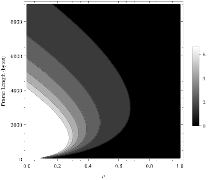
Figure 1: Contour plot of $h^{\prime\prime}(\rho)$ when $h(\rho)=\frac{\mathrm{T}_{\mathrm{off}}^{\text{frame}}(\rho)}{\mathrm{T}_{\mathrm{off}}^{\text{frame}}(\rho)+\mathrm{T}_{\mathrm{s}}+\mathrm{T}_{\mathrm{w}}}$ for a Poisson arrival process under the frame transmission energy-saving algorithm.

IV-A2 General traffic distributions

For unknown traffic distributions we must resort to the approximation given by (8), so we let $f(\rho)=1/(\mu\rho)-\mathrm{T}_{\mathrm{s}}$ and $b=\mathrm{T}_{\mathrm{s}}+\mathrm{T}_{\mathrm{w}}$. Now we can immediately substitute in $f^{\prime\prime}(\rho)(f(\rho)+b)>2(f^{\prime}(\rho))^{2}$ and get

$$\frac{2\bigl{(}\frac{1}{\mu\rho}+\mathrm{T}_{\mathrm{w}}\bigr{)}}{\mu\rho^{3}}>\frac{2}{\mu^{2}\rho^{4}}.$$ (13)

After some straightforward cancellations, this is

$$\frac{2\mathrm{T}_{\mathrm{w}}}{\mu\rho^{3}}>0,$$ (14)

which is obviously true.

IV-B Burst Transmission

Burst transmission is a simple modification of frame transmission that waits until a given number of packets $\mathrm{Q}_{\mathrm{w}}$ arrive at the network interface before exiting idle mode. To avoid excessive delays, there is a tunable parameter $\mathrm{T}_{\mathrm{\max}}$ that limits the wait for the $\mathrm{Q}_{\mathrm{w}}$-th frame since the first frame arrives. The analysis of the burst transmission algorithm is more involved, for the reason that there is not one but two operating regimes depending on the traffic load. Fortunately, [13] shows that the two operating regimes (low and high traffic load, respectively) can be neatly separated by the approximate traffic threshold

$$\rho^{\ast}\approx\frac{\mathrm{Q}_{\mathrm{w}}-1}{\mu\mathrm{T}_{\mathrm{\max}}},$$ (15)

where $\mathrm{Q}_{\mathrm{w}}$ and $\mathrm{T}_{\mathrm{\max}}$ are the tunable parameters in the burst transmission algorithm [11]. As in the previous Section, we will proceed and check whether, with burst transmission, the link energy consumption function is concave.

IV-B1 Low load regime, $\rho<\rho^{\ast}$

When the traffic load is low, the interface exits the low power mode before a backlog of $\mathrm{Q}_{\mathrm{w}}$ packets accumulates at the queue due to the timer expiry after waiting for $\mathrm{T}_{\mathrm{\max}}$ seconds. The exact expression for the expected sojourn time in the low-power state is (see [13])

$$\mathrm{T}_{\mathrm{off}}^{\text{burst, low}}(\rho)=\int_{0}^{\infty}(t+\mathrm{T}_{\mathrm{\max}}-\mathrm{T}_{\mathrm{s}})f_{\rho,\mathrm{T}_{\mathrm{e}}}(t)\textrm{d}t.$$ (16)

When $f_{\rho,T_{\text{e}}}(t)$ is unknown, according to [13], (16) can be approximated by

$$\mathrm{T}_{\mathrm{off}}^{\text{burst, low}}(\rho)\approx\frac{1}{\mu\rho}+\mathrm{T}_{\mathrm{\max}}-\mathrm{T}_{\mathrm{s}}.$$ (17)

As in the frame transmission algorithm, there exist closed expressions for $\mathrm{T}_{\mathrm{off}}^{\text{burst, low}}(\rho)$ for some distributions, and remarkably (17) is exact with Poissonian arrivals.

Proving the concavity of $E(\rho)$ in this case is direct. First, note that $f(\rho)=\mathrm{T}_{\mathrm{off}}^{\text{burst, low}}(\rho)=\mathrm{T}_{\mathrm{off}}^{\text{frame}}(\rho)+\mathrm{T}_{\mathrm{\max}}$, so that the derivatives $f^{\prime}$ and $f^{\prime\prime}$ are the same as in the frame transmission case, and hence plugging (17) into the condition $f^{\prime\prime}(x)(f(x)+b)>2(f^{\prime}(x))^{2}$ one can easily check that the inequality holds.

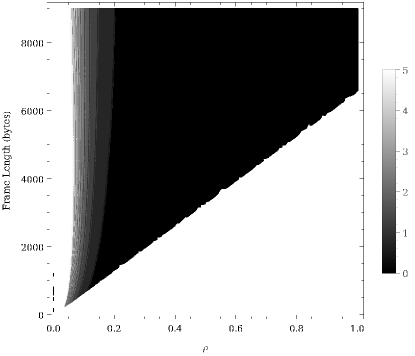
(a) Low load regime

(b) High-load regime

Figure 2: Contour plots of $h^{\prime\prime}(\rho)$ when $h(\rho)=\frac{\mathrm{T}_{\mathrm{off}}^{\text{burst}}(\rho)}{\mathrm{T}_{\mathrm{off}}^{\text{burst}}(\rho)+\mathrm{T}_{\mathrm{s}}+\mathrm{T}_{\mathrm{w}}}$ for a Poisson arrival process under the burst transmission energy-saving algorithm.

IV-B2 High load regime, $\rho>\rho^{\ast}$

When the traffic load is high, the packet burst is much more likely to reach its maximum size $\mathrm{Q}_{\mathrm{w}}$ before the timer expires. Now, the expected sojourn time in the low-power state is given by

$$\mathrm{T}_{\mathrm{off}}^{\text{burst,high}}(\rho)=\int_{\mathrm{T}_{\mathrm{s}}}^{\infty}(t-\mathrm{T}_{\mathrm{s}})f_{\rho,\mathrm{Q}_{\mathrm{w}}}(t)\textrm{d}t,$$ (18)

where, as usual, $f_{\rho,\mathrm{Q}_{\mathrm{w}}}(t)$ is the probability density function of the $\mathrm{Q}_{\mathrm{w}}$-th frame arrival epoch after the interface has entered the idle mode. When the density is unknown, according to [13] the expected time can be well approximated by

$$\mathrm{T}_{\mathrm{off}}^{\text{burst,high}}(\rho)\approx\frac{\mathrm{Q}_{\mathrm{w}}}{\mu\rho}-\mathrm{T}_{\mathrm{s}},$$ (19)

whereas the exact formula for the case of Poissonian arrivals is

$$\mathrm{T}_{\mathrm{off}}^{\text{burst,high}}(\rho)=\frac{\Gamma(\mathrm{Q}_{\mathrm{w}}+1,\mu\rho\mathrm{T}_{\mathrm{s}})-\mu\rho\mathrm{T}_{\mathrm{s}}\Gamma(\mathrm{Q}_{\mathrm{w}},\mu\rho T_{s})}{\mu\rho\Gamma(\mathrm{Q}_{\mathrm{w}})}.$$ (20)

Here, $\Gamma(\cdot)$ and $\Gamma(\cdot,\cdot)$ are the complete and incomplete Gamma functions [30], respectively.

In order to prove that Poissonian arrivals lead to concave energy consumption functions, simply substitute (20) into (6) to obtain after some straightforward calculations the inequality

$$\begin{split}\mu\rho\Gamma(\mathrm{Q}_{\mathrm{w}})^{2}\textrm{e}^{\mu\rho\mathrm{T}_{\mathrm{s}}}\Bigl{(}\mathrm{T}_{\mathrm{s}}(\mu\rho\mathrm{T}_{\mathrm{s}})^{\mathrm{Q}_{\mathrm{w}}}\bigl{(}(\mathrm{Q}_{\mathrm{w}}-\mu\rho\mathrm{T}_{\mathrm{s}})\Gamma(\mathrm{Q}_{\mathrm{w}},\mathrm{T}_{\mathrm{s}})+\\ \mu\rho(\mathrm{T}_{\mathrm{s}}+\mathrm{T}_{\mathrm{w}})\Gamma(\mathrm{Q}_{\mathrm{w}})\bigr{)}+\\ 2\textrm{e}^{\mu\rho\mathrm{T}_{\mathrm{s}}}\Gamma(\mathrm{Q}_{\mathrm{w}}+1,\mu\rho\mathrm{T}_{\mathrm{s}})\bigl{(}(\mathrm{T}_{\mathrm{s}}+\mathrm{T}_{\mathrm{w}})\Gamma(\mathrm{Q}_{\mathrm{w}})-\\ \mathrm{T}_{\mathrm{s}}\Gamma(\mathrm{Q}_{\mathrm{w}},\mu\rho\mathrm{T}_{\mathrm{s}})\bigr{)}\Bigr{)}>0.\end{split}$$ (21)

All the constant terms appearing in the above inequality are positive, so this simplifies somewhat to

$$\begin{split}\mathrm{T}_{\mathrm{s}}(\mu\rho\mathrm{T}_{\mathrm{s}})^{\mathrm{Q}_{\mathrm{w}}}\Bigl{(}\mu\rho\bigl{(}(\mathrm{T}_{\mathrm{s}}+\mathrm{T}_{\mathrm{w}})\Gamma(\mathrm{Q}_{\mathrm{w}})-\mathrm{T}_{\mathrm{s}}\Gamma(\mathrm{Q}_{\mathrm{w}},\mu\rho\mathrm{T}_{\mathrm{s}})\bigr{)}+\\ \Gamma(\mathrm{Q}_{\mathrm{w}}+1,\mu\rho\mathrm{T}_{\mathrm{s}})\Bigr{)}+\\ \Gamma(\mathrm{Q}_{\mathrm{w}}+1,\mathrm{T}_{\mathrm{s}}\mu\rho)\bigl{(}(\mathrm{T}_{\mathrm{s}}+\mathrm{T}_{\mathrm{w}})\Gamma(\mathrm{Q}_{\mathrm{w}})-\mathrm{T}_{\mathrm{s}}\Gamma(\mathrm{Q}_{\mathrm{w}},T_{s}\mu\rho)\bigr{)}>0\end{split}$$ (22)

which holds true because

$$\mu\rho(\mathrm{T}_{\mathrm{s}}+\mathrm{T}_{\mathrm{w}})\Gamma(\mathrm{Q}_{\mathrm{w}})>\mu\rho\mathrm{T}_{\mathrm{s}}\Gamma(\mathrm{Q}_{\mathrm{w}})>\mu\rho\mathrm{T}_{\mathrm{s}}\Gamma(\mathrm{Q}_{\mathrm{w}},\mu\rho\mathrm{T}_{\mathrm{s}})$$ (23)

as a consequence of elementary properties of the Gamma functions. This implies that all the summands in the left side of (22) are positive, and (6) is satisfied.

The last step is to prove concavity for the general approximation (19). A change of variable $m=\mathrm{Q}_{\mathrm{w}}/\rho$ transforms (19) into (8) formally. Since $m>0$, following the same steps as in frame transmission, one concludes that (19) also fulfills condition (6). Hence, the link energy consumption function $E(\cdot)$ is concave with burst transmission in the high-load regime, regardless the traffic arrival pattern.

A numerical illustration of the concavity is shown in Fig. 2, which depicts the contour plots of $h^{\prime\prime}(\rho)$ for a $10$ Gb/s Ethernet link as the traffic load and the packet size vary.

V Delay Control

According to the previous sections, a straightforward application of a water-filling algorithm to share traffic among the bundle links provides maximum energy savings. However, if proper care is not taken, packet delay can grow uncontrolled as we explain next.

From a practical point of view there are many ways to implement a water filling algorithm. For instance, one could use separate queues for each link and only divert traffic to new links when the queue of the previous one overflows. Obviously, this approach exhibits the greatest delay. A second option is to limit the load factor in every link, and thus the delay, and divert traffic when this threshold is reached. Its main drawback is that no link is used at its full capacity and so the energy savings are not maximum. Another option, in the opposite extreme, is to have a common bundle queue and zero-length queues at the links. In this case, a new link is used if when a packet arrives, the previous link is busy transmitting a packet. The problem is that if the traffic load is not high enough, we will find that the first link is idle while the second one is transmitting, and that goes against the idea of the water-filling algorithm.

We propose a simple dynamic water-filling algorithm that can control average delay, while keeping the utilization factor of the links close to 1. The algorithm has one configuration parameter, the expected delay ($d_{e}$) and $N+1$ state variables, with $N$ the number of links in the bundle, as it just keeps a record of the short term average delay ($d_{av}$), calculated with an exponentially weighted moving average, and the current queue length in each link measured in time units ($q_{i},\,i=1\ldots N$). More precisely, when a new packet is about to get queued in queue $i$, the current average delay value $d_{av}^{\prime}$ is updated as

$$d_{av}^{\prime}=\beta q_{i}+(1-\beta)d_{av},\,0<\beta<1,$$ (24)

where $q_{i}^{j}$ is the $q_{i}$ value when the $j$-th packet arrives, calculated as the amount of traffic stored in the $i$-th queue over the link capacity, and $\beta$ is a gain factor. Updating $d_{av}$ on packet arrivals avoids the need to record and store the arrival time of every packet to the system.

The algorithm works as follows. Each link in the bundle is assumed to have its own queue, so whenever a new packet arrives, the algorithm decides which queue should store it. For this the expected delay is compared with the current average delay. If $d_{av}<d_{e}$, the packet is stored in the queue of the first link. For every other case, a sequential search is started for a queue with a queue length smaller than the expected delay. If no queue is found, the packet is stored in the last queue. This is all summarized in Listing 1.

⬇

1function packet_arrival

2 if ($d_{av}$ < $d_{e}$)

3 return enqueue(Links[$1$])

4

5 foreach ($\ell$ in Links)

6 if ($q_{\ell}$ < $d_{e}$)

7 return enqueue($\ell$)

8

9 return enqueue(N)

Listing 1: Dynamic water-filling algorithm.

VI Results

We have carried out several experiments to assess the effectiveness of our proposed sharing strategy. We have employed the ns-2 network simulator with an added module for simulating IEEE 802.3az links available for download at [31]. The simulated bundles have a varying number of 10 Gb$/$s links with 10GBASE-T interfaces, so $\mathrm{T}_{\mathrm{s}}=2.88\,\mu$s, $\mathrm{T}_{\mathrm{w}}=4.48\,\mu$s and $\sigma_{\mathrm{off}}=0.1$, in accordance with several estimates provided by different manufactures during the standardization process of the IEEE 802.3az standard. For the burst transmission simulations we set up $\mathrm{T}_{\mathrm{\max}}=100\,\mu$s and $\mathrm{Q}_{\mathrm{w}}=20\,$frames, so that $\mu\mathrm{T}_{\mathrm{s}}>3.6\,$frames, as recommended in [13].

VI-A Model Validation

The first set of experiments tests all possible traffic sharing alternatives in a simple 2-link bundle when it is fed with synthetic traffic. For the experiments we used a fixed frame size of 1000 bytes and a varying arrival rate, so that the aggregated load ranged between 25 and 175%. Then, for each load we modified the share between the two links and, for each share, we run five simulations with different random seeds and a ten seconds duration.

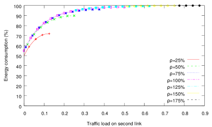
(a) Frame transmission

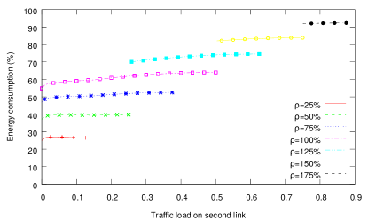
(b) Burst transmission

Figure 3: Results for a 2-link bundle with Poisson traffic as a function of excess traffic load on the second link.

Figure 3 shows the total energy consumption of the bundle versus the traffic load on the second link for Poisson traffic with both the frame and burst transmission algorithms. For clarity, we take advantage of the symmetry of the problem and only represent the results where load on the second link is smaller than that on the first. Thus, for each experiment the leftmost value represents the water-fill algorithm, with most of the traffic on the first link, while the rightmost value corresponds with an equal share of traffic among both links. Figure 3 shows very clearly that there is very little variance among the different simulations for the same share and load and, at the same time, that the results match those provided by the model, plotted with continuous lines in the graph. It is also easy to see the increasing energy consumption with the traffic load on the second link. The closer the loads of both links are, the higher the energy needs. In fact, the minimum consumption is obtained when most load is concentrated on a single link, as predicted. Finally, we also observe that the benefit of aggregating load on a single link is much greater for frame than for burst transmission. This is a consequence of the fact that the energy profile of the burst transmission algorithm is more linear [7]. Thus, there is less sensitivity to how the traffic load is shared among the links of the bundle —note that total energy consumption shows little variations when the traffic share is modified in Fig. 3(b)—. Also, as expected, burst transmission needs less energy than frame transmission.

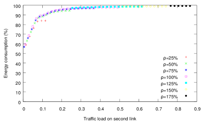
(a) Frame transmission

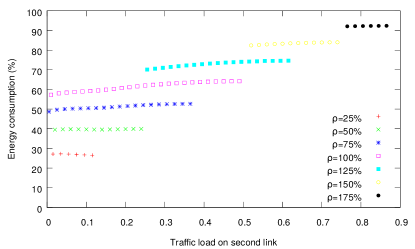
(b) Burst transmission

Figure 4: Results for a 2-link bundle with Pareto traffic as a function of excess traffic load on the second link. Theoretical values omitted, as there is no closed form formula for Pareto arrivals [13].

The results for Pareto traffic (with the shape factor $\alpha$ set to $2.5$) are plotted in Fig. 4. Although the performance curves are not as smooth as for the Poisson traffic, the previous conclusions still hold. Again, the minimum consumption is obtained when most of the traffic is on a single link and then increases as the traffic on the second link increases. At the same time, the frame transmission algorithm benefits more than the burst transmission one.

Our second experiment compares the overall energy consumption of an Ethernet bundle for the full range of possible incoming traffic demands and two different sharing methods. The first spreads the traffic evenly across all the constituent links, denoted in the results by equitable, while the second is the naïve water-filling method. Traffic follows a Poisson distribution and the frame size is 1000 bytes, as in the previous experiment. Figure 5 displays both the experimental and analytic results for two, four and eight-link aggregates. Again, frame transmission algorithm benefits more than burst transmission of the water-fill sharing algorithm. Further, as the number of links in the bundle increases, the energy demands of frame transmission, when using the water-fill procedure, approximate those of burst transmission.

VI-B Dynamic Water-filling Algorithm

The next set of experiments tests the behavior of the dynamic water-filling algorithm. We have employed real traffic traces captured on Internet backbones for the simulations. The traffic comes from the publicly available passive monitoring CAIDA dataset from 2013 [32] which provides anonymized traces from a 10 Gb$/$s Internet backbone. We used one of these traces to feed traffic to a simulated 4-link bundle made of 10GBASE-T interfaces. Of all the available traces, we have chosen one with a relatively high demand of about 6 Gb$/$s on average. As that load is still quite low for our simulated bundle of 40 Gb$/$s we made new traces of approximately 12, 18, 24 and 30 Gb$/$s combining traffic from additional independent adjacent traces. For this we concatenated the traces and then reduced the inter-arrival times by a constant factor (2, 3, 4 and 5 respectively). We proceeded in this manner to keep any existing auto-correlation in the final traces. Finally, we have chosen $\beta=0.1$ as the gain factor in (24).

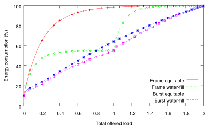
(a) Two links bundle

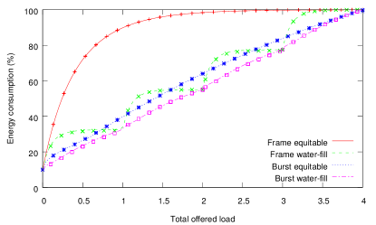
(b) Four links bundle

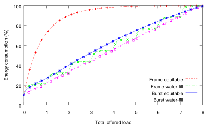
(c) Eight links bundle

Figure 5: Normalized global consumption of a bundle link for the different idle mode governors.

The first experiment verifies that the proposed dynamic algorithm is in fact able to control the average delay. For this we have fed all the traffic traces to a 4-link bundle, and configured the algorithm for different expected delays. The results are plotted in Fig. 6. It can be clearly seen an almost perfect relationship between the configured and the measured average delay for values greater than the transition times of the EEE links. The exception is the 6 Gb$/$s trace, that is bounded below 4$\,\mu$s. This is expected, as the queue cannot grow larger when the capacity of a single link is greater than the offered traffic. The simulation with the 12 Gb$/$s trace shows a small drift of the average delay, but, in any case, the average delay is kept below the configured delay. This error in the 12 Gb$/$s experiment occurs because (24) can overestimate average queuing delay if waiting time samples from low used queues are few and far between them, so the samples from the first queue get over-represented. Although omitted for brevity, decreasing the $\beta$ value lessens the drift.

Figure 6: Obtained average delay versus configured delay for the dynamic water-fill algorithm.

The second experiment shows the variation of power consumption versus expected delay. The results are shown in Fig. 7. When the expected delay is too low, all links are used simultaneously, and the power savings are minimal. However, as the allowed delay increases, most of the traffic is transmitted by the first links and, despite the fact that all of them are powered on, we achieve large power savings thanks to the concavity of the cost function. It is important to notice that the maximum energy savings are already obtained starting from low delay target values. This allows to deploy the algorithm even in networks used by delay-sensitive applications.

Figure 7: Power consumption versus expected delay for the dynamic water-fill algorithm.

In the last experiment we have compared the results obtained when sharing the traffic with three different strategies: spreading the traffic evenly across the four links, that we called equitable, a naïve implementation of the water-fill algorithm and, finally, the dynamic water-fill algorithm with a target delay of ten microseconds for the frame transmission algorithm and 20$\,\mu$s for the burst one. For the naïve implementation we have constrained the traffic load on any link to 90% to avoid excessive buffering.

Bundle	Strategy	Link #1	Link #2	Link #3	Link #4
	Equit.	$1.55$	$1.55$	$1.55$	$1.55$
$6.21$	Naïve Water-fill	$6.21$	0	0	0
	Dyn. Frame	$6.21$	0	0	0
	Dyn. Burst	$6.18$	$0.03$	0	0
	Equit.	$3.15$	$3.15$	$3.15$	$3.15$
$12.60$	Naïve Water-fill	$9$	$3.60$	0	0
	Dyn. Frame	$9.44$	$3.08$	$0.07$	0
	Dyn. Burst	$9.50$	$2.67$	$0.39$	$0.04$
	Equit.	$4.71$	$4.70$	$4.70$	$4.70$
$18.81$	Naïve Water-fill	$9$	$9$	$0.81$	0
	Dyn. Frame	$9.94$	$7.12$	$1.73$	$0.02$
	Dyn. Burst	$9.97$	$6.82$	$1.77$	$0.25$
	Equit.	$6.27$	$6.27$	$6.27$	$6.27$
$25.08$	Naïve Water-fill	$9$	$9$	$7.08$	0
	Dyn. Frame	$10$	$9.16$	$5.12$	$0.80$
	Dyn. Burst	$10$	$9.13$	$4.78$	$1.17$
	Equit.	$7.85$	$7.85$	$7.85$	$7.85$
$31.40$	Naïve Water-fill	$9$	$9$	$9$	$4.4$
	Dyn. Frame	$10$	$9.82$	$7.94$	$3.64$
	Dyn. Burst	$10$	$9.83$	$7.74$	$3.83$

Table I: Average traffic fed into each link for the real traffic simulations (in Gb$/$s).

The exact traffic rate of each trace and the different shares are detailed in Table I. For the equitable and the naïve water-fill they have been determined beforehand, but for the dynamic algorithm the table lists the results obtained via simulation. The results for both the frame transmission and the burst transmission algorithms are depicted in Fig. 8.

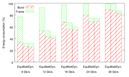
Figure 8: Energy consumption with real traffic traces when employing different strategies to share the traffic in a 4-link bundle.

In every case the frame transmission algorithm needs more energy than the burst transmission one, but, at the same time, the savings resulting from applying the water-fill procedure are also greater. In fact, there is usually very little difference in the consumption of both EEE algorithms in that case. As expected, the equitable share draws more energy than the other two shares and the water-fill share is the one that produces the best results. Finally, the dynamic water-fill algorithm improves the results, but not substantially.

We have also measured the impact of the different algorithms on queuing delay. Figure 9 shows the average queuing delay suffered by the traffic in the previous experiment.

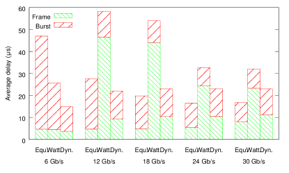
Figure 9: Average queuing delay with real traffic traces when employing different strategies to share the traffic in a 4-link bundle.

As it is the case for single EEE links [13], we observe that burst transmission always causes more delay than frame transmission. We also find that the different sharing methods impact on the queuing delay differently. In the 6 Gb$/$s case, the equitable share produces the highest delays with burst transmission, as there is relatively little traffic in every link, and thus packets have to wait for $Q_{w}$ packets to arrive before being transmitted. In every other case, the naïve water-fill algorithm produces the longest packet delays, as at least one queue is driven near its full capacity. Finally, the dynamic algorithm produces stable delays, near its target —10$\,\mu$s for frame and $20\,\mu$s for burst transmission— that are in the same range as those of the equitable share.

VII Conclusions

This paper presents an optimum, yet simple, procedure for distributing traffic load among the links of a bundle that minimizes energy consumption when individual links employ an EEE algorithm. As explained, the maximum energy savings are obtained when traffic is only transmitted on a link if all the previous ones in the aggregate are already being used at their maximum allowed load. The paper proves the optimality of the procedure for typical energy cost functions of individual Ethernet links.

The provided procedure is oblivious of the energy saving algorithm used in the links, whether it is the simple frame transmission algorithm or the more efficient burst transmission one. Moreover, we found that as the number of links forming the bundle increases, the difference in the total energy consumption between both algorithms vanishes when using our sharing procedure. Thus, for bundles made up of many links it is advisable to use the simpler frame transmission algorithm in the links, as it both reduces complexity and adds less latency to the transmitted frames.

We have also explored several alternatives to build a practical implementation of the water-filling idea to then present a simple practical implementation that is able to keep average delay controlled at a configurable target value while minimizing overall energy consumption. The algorithm requires little memory and computational power, so that a vendor can implement it just by modifying the firmware of the Ethernet line card. However, as the algorithm needs to obtain the queue occupation of each port to classify incoming packets, an open-flow implementation is not currently possible, as the current spec [33] does not define the needed counters. Future research could explore the possibility of extending the current spec to empower the user with the fine grained control of the transmission ports needed by our proposal.

Finally, we have tested our procedure with both synthetic and real traffic traces. In all cases, the obtained results match our expectations with the best results being obtained when the proposed sharing algorithm is employed, reducing energy consumption as much as $50\,$%.

Appendix A Proof of proposition 1

In this Section, we prove that for the particular case of equal cost functions the solution to the optimum allocation is a simple sequential water-filling algorithm: each link capacity is fully used before sending traffic through a new, idle link.

We assume $X<\sum_{i}C_{i}$, otherwise the solution is trivial. It is easy to see that the constraints define a convex region $\mathcal{R}$. Since the objective function is concave, it follows that it attains its minimum at some of the extreme points of $\mathcal{R}$, namely $x_{i}=C_{i}$ for $i\in T\subseteq[1:N],\quad 0<x_{j}<C_{j}$ for one $j\in[1:N]$ and $x_{k}=0$ for all $k\in T^{C}\setminus\{j\}$. In fact, when all the cost functions are equal, the optimal traffic allocation is to use the links in decreasing order of capacity. Assume, without loss of generality, that $C_{1}>C_{2}>\ldots>C_{N}$. Fix two links $i$ and $j$, $i>j$, and assume that a feasible solution is the vector $\mathbf{x}=(x_{i}^{*},\ldots,x_{N}^{*})$. Then, since $E$ is a concave function it is also subadditive, and for $i>j$ and $\delta<\min\{x_{i}^{*},C_{j}-x_{j}^{*}\}$ we have

$$E(x_{i}^{*})+E(x_{j}^{*})\geq E(x_{i}^{*}-\delta)+E(x_{j}^{*}+\delta).$$ (25)

Therefore, the vector $\tilde{\mathbf{x}}=(x_{1}^{*},\ldots,x_{j}^{*}+\delta,\ldots,x_{i}^{*}-\delta,\ldots,x_{N}^{*})$ is a better solution than $\mathbf{x}$. Iterating this argument as many times as necessary, it is immediate to conclude that

$$x_{i}^{*}=C_{i}\text{ for }i=1,\ldots,s-1$$ (26)

$$0\leq x_{s}^{*}=X-\sum_{i=1}^{s-1}C_{i}<C_{s}$$ (27)

$$x_{j}^{*}=0\text{ for }j=s+1,\ldots,N$$ (28)

is the optimal solution, where $\sum_{i=1}^{s-1}C_{i}\leq X<\sum_{i=1}^{s}C_{i}.\qed$

To see (25), recall that for a concave function $f$ and three ordered points $a<b<c$ it holds

$$\frac{f(b)-f(a)}{b-a}\geq\frac{f(c)-f(a)}{c-a}.$$ (29)

Just let $t=(b-a)/(c-a)$ so that $b=(1-t)a+tc$. By the definition of concavity

$$f(b)\geq(1-t)f(a)+tf(c),$$ (30)

which is (29). Similarly, for $a<b<c$

$$\frac{f(c)-f(a)}{c-a}\geq\frac{f(c)-f(b)}{c-b},$$ (31)

and combining (29) and (31) gives

$$\frac{f(b)-f(a)}{b-a}\geq\frac{f(c)-f(b)}{c-b}.$$ (32)

Now, use inequality (32) twice over the tuples $(x_{i}-\delta,x_{i},x_{j})$ and $(x_{i},x_{j},x_{j}+\delta)$ to conclude (25).∎

Appendix B Proof of proposition 2

Consider the auxiliary function

$$u(x)=1-t(x)=a(1-x)\frac{f(x)}{f(x)+b}=g(x)h(x),$$ (33)

where $g(x)\triangleq a(1-x)$ and $h(x)\triangleq f(x)/(f(x)+b)$. Strict concavity of $t(x)$ is equivalent to $u(x)$ being strictly convex or, alternatively, to $u^{\prime\prime}(x)>0$. Taking the second derivative of $u(x)$ we get

$$u^{\prime\prime}(x)=g(x)h^{\prime\prime}(x)-2ah^{\prime}(x),$$ (34)

because $g^{\prime}(x)=-a$. So, $u(x)$ is strictly convex if and only if $g(x)h^{\prime\prime}(x)>2ah^{\prime}(x)$. But

$$h^{\prime}(x)=b\frac{f^{\prime}(x)}{\bigl{(}f(x)+b\bigr{)}^{2}}<0,$$ (35)

since we assumed $f(x)$ to be decreasing. With $g(x)>0$ for $x\in[0,1]$, $a>0$ and (35), (34) shows that $h(x)$ convex implies $u(x)$ convex. Finally,

$$h^{\prime\prime}(x)=b\frac{f^{\prime\prime}(x)\bigl{(}f(x)+b\bigr{)}-2\bigl{(}f^{\prime}(x)\bigr{)}^{2}}{\bigl{(}f(x)+b\bigr{)}^{3}},$$ (36)

and $h(x)$ is a convex function —$t(x)$ is a concave function— if and only if $f^{\prime\prime}(x)(f(x)+b)>2(f^{\prime}(x))^{2}$, since $f(x)$ is nonnegative.∎

References

- [1] S. Lambert, W. V. Heddeghem, W. Vereecken, B. Lannoo, D. Colle, and M. Pickavet, “Worldwide electricity consumption of communication networks,” Optics Express, vol. 20, no. 26, pp. 513–524, Dec. 2012.
- [2] B. Heller, S. Seetharaman, P. Mahadevan, Y. Yiakoumis, P. Sharma, S. Banerjee, and N. McKeown, “Elastictree: Saving energy in data center networks,” in USENIX Symposium on Networked Systems Design and Implementation, NSDI 2010, San Jose, CA, USA, Apr. 2010, pp. 249–264.
- [3] “IEEE 802.3az,” Oct. 2010. [Online]. Available: http://dx.doi.org/10.1109/IEEESTD.2010.5621025
- [4] M. Gupta and S. Singh, “Using low-power modes for energy conservation in Ethernet LANs,” in Proceedings of the IEEE INFOCOM, Anchorage, AK; USA, 2007, pp. 2451–2455.
- [5] M. Rodríguez Pérez, S. Herrería Alonso, M. Fernández Veiga, and C. López García, “Improved opportunistic sleeping algorithms for LAN switches,” in Proceedings of the IEEE Globecom, Honolulu, HI, USA, Dec. 2009.
- [6] P. Reviriego Vasallo, J. A. Maestro, J. A. Hernández, and D. Larrabeiti, “Burst transmission for Energy-Efficient Ethernet,” IEEE Internet Computing, vol. 14, no. 4, pp. 50–57, Jul. 2010.
- [7] K. Christensen, P. B. N. Reviriego Vasallo, M. Bennett, M. Mostowfi, and J. A. Maestro, “IEEE 802.3az: the road to energy efficient Ethernet,” IEEE Communications Magazine, vol. 48, no. 11, pp. 50–56, 2010.
- [8] P. Reviriego Vasallo, J. A. Hernández, D. Larrabeiti, and J. A. Maestro, “Performance evaluation of Energy Efficient Ethernet,” IEEE Communications Letters, vol. 13, no. 9, pp. 697–699, Sep. 2009.
- [9] P. Reviriego Vasallo, K. Christensen, J. Rabanillo, and J. A. Maestro, “An initial evaluation of energy efficient Ethernet,” IEEE Communications Letters, vol. 15, no. 5, pp. 578–580, May 2011.
- [10] S. Herrería Alonso, M. Rodríguez Pérez, M. Fernández Veiga, and C. López García, “Opportunistic power saving algorithms for Ethernet devices,” Computer Networks, vol. 55, no. 9, pp. 2051–2064, Jun. 2011.
- [11] ——, “A power saving model for burst transmission in energy-efficient Ethernet,” IEEE Communications Letters, vol. 15, no. 5, pp. 584–586, May 2011.
- [12] M. A. Marsan, A. F. Anta, V. Mancuso, B. Rengarajan, P. Reviriego Vasallo, and G. Rizzo, “A simple analytical model for energy efficient Ethernet,” IEEE Communications Letters, vol. 15, no. 7, pp. 773–775, Jul. 2011.
- [13] S. Herrería Alonso, M. Rodríguez Pérez, M. Fernández Veiga, and C. López García, “A GI/G/1 model for 10 Gb/s energy efficient Ethernet,” IEEE Transactions on Communications, vol. 60, pp. 3386–3395, Nov. 2012.
- [14] M. Aksić and M. Bjelica, “Packet coalescing strategies for energy-efficient Ethernet,” Electronics Letters, vol. 50, no. 7, pp. 521–523, Mar. 2014.
- [15] “IEEE Std 802.1ax IEEE standard for local and metropolitan area networks — link aggregation,” pp. 1–145, Nov. 2008.
- [16] M. Gupta and S. Singh, “Greening of the Internet,” in SIGCOMM’03: Proceedings of the 2003 conference on Applications, technologies, architectures, and protocols for computer communications, no. 4. ACM, 2003, pp. 19–26.
- [17] L. Chiaraviglio, M. Mellia, and F. Neri, “Minimizing ISP network energy cost: Formulation and solutions,” IEEE/ACM Transactions on Networking, vol. 20, no. 2, pp. 463–476, Apr. 2012.
- [18] B. Addis, A. Capone, G. Carello, L. Gianoli, and B. Sanso, “Energy management through optimized routing and device powering for greener communication networks,” IEEE/ACM Transactions on Networking, vol. 22, no. 1, pp. 313–325, Feb 2014.
- [19] R. G. Garroppo, S. Giordano, G. Nencioni, and M. Pagano, “Energy aware routing based on energy characterization of devices: Solutions and analysis,” in Communications Workshops (ICC), 2011 IEEE International Conference on, 2011, pp. 1–5.
- [20] R. Garroppo, G. Nencioni, L. Tavanti, and M. G. Scutellà, “Does traffic consolidation always lead to network energy savings?” IEEE Communications Letters, vol. 17, no. 9, pp. 1852–1855, Sep. 2013.
- [21] J. Galán Jiménez and A. Gazo Cervero, “Using bio-inspired algorithms for energy levels assessment in energy efficient wired communication networks,” Journal of Network and Computer Applications, vol. 37, pp. 171–185, Jan. 2014.
- [22] C. Gunaratne, K. Christensen, S. W. Suen, and B. Nordman, “Reducing energy consumption of Ethernet with an adaptive link rate (ALR),” IEEE Transactions on Computers, vol. 57, no. 4, pp. 448–461, Apr. 2008.
- [23] D. Larrabeiti, P. Reviriego, J. Hernández, J. Maestro, and M. Uruea, “Towards an energy efficient 10 Gb/s optical Ethernet: Performance analysis and viability,” Optical Switching and Networking, vol. 8, no. 3, pp. 131–138, 2011.
- [24] R. Bolla, R. Bruschi, A. Carrega, F. Davoli, and P. Lago, “A closed-form model for the IEEE 802.3az network and power performance,” IEEE Journal on Selected Areas in Communications, vol. 32, no. 1, pp. 16–27, 2014.
- [25] S. Herrería Alonso, M. Rodríguez Pérez, M. Fernández Veiga, and C. López García, “Optimal configuration of energy-efficient Ethernet,” Computer Networks, vol. 56, no. 10, pp. 2456–2467, Jul. 2012.
- [26] A. Cenedese, M. Michielan, F. Tramarin, and S. Vitturi, “An energy efficient traffic shaping algorithm for Ethernet-based multimedia industrial traffic,” in Emerging Technology and Factory Automation (ETFA), 2014 IEEE, Sep. 2014, pp. 1–4.
- [27] S. Vitturi and F. Tramarin, “Energy efficient ethernet for real-time industrial networks,” IEEE Transactions on Automation Science and Engineering, vol. 12, no. 1, pp. 228–237, 2015.
- [28] T. Karagiannis, M. Molle, M. Faloutsos, and A. Broido, “A nonstationary Poisson view of Internet traffic,” in Proceedings of the IEEE INFOCOM, vol. 3, 2004, pp. 1558–1569.
- [29] A. Vishwanath, V. Sivaraman, and D. Ostry, “How Poisson is TCP traffic at short time-scales in a small buffer core network,” in IEEE 3rd Intl. Symp on Advanced Networks and Telecommunication Systems (ANTS), 2009, Dec. 2009, pp. 1–3.
- [30] M. Abramowitz and S. I.A., Handbook of mathematical functions. New York, USA: Dover, 1972.
- [31] “ns Network Simulator v2.35 with IEEE802.3az support,” https://github.com/migrax/ns2/commits/ieee802.3az, Feb. 2014.
- [32] “The CAIDA UCSD anonymized 2013 Internet traces — 2013/08/15 13:14:00 UTC,” https://www.caida.org/data/passive/passive_2013_dataset.xml.
- [33] The Open Networking Foundation, “Openflow switch specifiation,” Oct. 2013, version 1.4.0. [Online]. Available: https://www.opennetworking.org/images/stories/downloads/sdn-resources/onf-specifications/openflow/openflow-spec-v1.4.0.pdf