Discontinuous dynamics with grazing points

Abstract

Discontinuous dynamical systems with grazing solutions are discussed. The group property, continuation of solutions, continuity and smoothness of motions are thoroughly analyzed. A variational system around a grazing solution which depends on near solutions is constructed. Orbital stability of grazing cycles is examined by linearization. Small parameter method is extended for analysis of neighborhoods of grazing orbits, and grazing bifurcation of cycles is observed in an example. Linearization around an equilibrium grazing point is discussed. The mathematical background of the study relies on the theory of discontinuous dynamical systems [1]. Our approach is analogous to that one of the continuous dynamics analysis and results can be extended on functional differential, partial differential equations and others. Appropriate illustrations with grazing limit cycles and bifurcations are depicted to support the theoretical results.

Keywords: Discontinuous dynamical systems; Grazing points and orbits; Axial and non-axial grazing; Variational system; Orbital stability; Small parameter; Bifurcation of cycles; Impact mechanisms

1 Introduction

Vibro-impacting systems provide examples of non-linear dynamical systems, exhibiting new levels of complicated dynamics due to their non-smoothness. Grazing phenomenon is one of the attractive features for these dynamics [13]-[36], [26]-[29]. There are two approaches for the definition of grazing in literature. One is presented in the studies of Bernardo, Budd and Champneys [7, 8], Bernardo and Hogan [9], and Luo [26]-[29]. In these studies, it is asserted that grazing occurs when a trajectory hits the surface of discontinuity tangentially. In [36]-[39], Nordmark defines grazing as the approach of the velocity to zero in the neighborhood of the surface of discontinuity which is the case of the studies conducted in [7]-[9], [26]-[29]. Our comprehension of grazing in this paper is close to that one in [8],[9],[26]. In the paper [15], grazing is considered as a bounding case which separates regions of quite different dynamic behaviors. It is understood that the system trajectory makes tangential contact with an event triggering hypersurface. The shooting, continuation and optimization methods are developed and illustrated for both transient and grazing phenomena. It is exemplified by utilizing power electronics and robotics. In [41], the grazing periodic orbit and its linearization are obtained by means of a numerical continuation method for hybrid systems. Applying this, the normal-form coefficients are evaluated, which in this case imply the occurrences a jump to chaos and period-adding cascade. The necessary and sufficient conditions of the general discontinuous boundary are expounded in [28]. In [27], by means of non-stick mapping, the necessary and sufficient conditions for the grazing in periodically forced linear oscillator with dry friction are obtained. By constructing special maps such as zero time discontinuity mapping [10]-[12] and Nordmark map [36]-[39], the existence of periodic solution and their stability were investigated in mechanical systems.

In this paper, we model the dynamics with grazing impacts by utilizing differential equations with impulses at variable moments and applying the methods of [1]-[3]. As a consequence of such methods, the role of the mappings [36]-[39] is diminished. One can observe that a trajectory at a grazing point may have tangency to the surface of discontinuity, which is parallel to one or several coordinate axises. Particularly it means the velocity approaches to zero [36]-[39]. Then, we will say about the axial grazing. Otherwise, grazing is non-axial. This research contains the analysis of both axial and non-axial grazing.

In [33], it is observed through simulations and experiments that the coefficient of restitution depends on the impact velocity of the particle by considering both the viscoelastic and the plastic deformations of particles occurring at low and high velocities, respectively. It has been proposed in [32] that at low impact velocities and for most materials with linear elastic range, the coefficient of restitution is of the form $R(v)=1-av,$ where $v$ is the velocity before collision and $a$ is a constant. Also, for low impact velocities the restitution law can be considered quadratic [16]. This is why, we will use non-constant restitution coefficients in models with impacts in this study.

For investigation of autonomous differential equations, it is convenient to utilize properties of dynamical systems. They are the group property, continuation of solutions in both time directions, continuity and differentiability in parameters. The studies of discontinuous dynamical systems with transversal intersections of orbits and surfaces, $B-$ smooth discontinuous flows, can be found in [1, 2]. In this research, the dynamics is approved for systems with grazing orbits. Moreover, the definitions of orbital stability and asymptotic phase are adapted to grazing cycles. The orbital stability theorem is proved, which can not be underestimated for theory of impact mechanisms.

The remaining part of the paper is organized as follows. In the next section, we will introduce necessary notations, definitions and theorems to specify discontinuous dynamical systems. In Section 3, it is shown how the dynamics can be linearized around grazing orbits. In Section 4, the theorem of orbital stability is adapted for grazing cycles. In Section 5, the small parameter analysis is applied near grazing orbits and bifurcation of cycles is observed. In last three sections, examples are presented to actualize the theoretical results numerically and analytically. Finally, Conclusion covers a summary of our study.

2 Discontinuous dynamical systems

Let $\mathbb{R},$ $\mathbb{N}$ and $\mathbb{Z}$ be the sets of all real numbers, natural numbers and integers, respectively. Consider the set $D\in\mathbb{R}^{n}$ such that $D=\cup D_{i},$ where $D_{i},$ $i=1,2,\ldots,k,$ components of $D,$ are disjoint open connected subsets of $\mathbb{R}^{n}.$ To describe the surface of discontinuity, we present a two times continuously differentiable function $\Phi:D^{r}\rightarrow\mathbb{R}^{n}.$ The set can be defined as $\Gamma=\Phi^{-1}(0)$ and is a closed subset of $\bar{D},$ where $\bar{D}$ is the closure of $D.$ Denote $\partial\Gamma$ as the boundary of $\Gamma.$ One can easily see that $\Gamma=\cup_{i=1}^{k}\Gamma_{i}$, where $\Gamma_{i}$ are parts of the surface of discontinuity in the components of $D.$ Denote $\tilde{\Gamma}=J(\Gamma),$ $\tilde{\Phi}(x)=\Phi(J^{-1}(x)).$ Denote an $r-$ neighborhood of $D$ in $\mathbb{R}^{n}$ for a fixed $r>0$ as $D^{r}.$ Let $\Gamma^{r}$ be the $r-$ neighborhood of $\Gamma$ in $\mathbb{R}^{n},$ for a fixed $r>0$ and define functions $J:\Gamma^{r}\rightarrow D^{r}$ and $\tilde{J}:\tilde{\Gamma}^{r}\rightarrow D^{r},$ such that, $J(\Gamma),\tilde{J}(\tilde{\Gamma})\subset D.$ Assume that a function $f(x):D^{r}\rightarrow\mathbb{R}^{n}$ is continuously differentiable in $D^{r}.$ Set the gradient vector of $\Phi$ as $\nabla\Phi(x).$

The following definitions will be utilized in the remaining part of the paper. Let $x(t-)$ be the left limit position of the trajectory and $x(t+)$ be the right limit of the position of the trajectory at the moment $t.$ Define $\displaystyle{\Delta x(t):=x(t+)-x(t-)}$ as the jump operator for a function $x(t)$ such that $x(t)\in\Gamma$ and $t$ is a moment of discontinuity (discontinuity moment). In other words, the discontinuity moment $t$ is the moment when the trajectory meets the surface of discontinuity $\Gamma.$ The function $I(x)$ will be used in the following part of the paper which is defined as $I(x):=J(x)-x,$ for $x\in\Gamma.$

The following assumptions are needed throughout this paper.

• $\nabla\Phi(x)\neq 0$ for all $x\in\Gamma,$

• $J\in C^{1}(\Gamma^{r})$ and $\det\Big{[}\frac{\partial J(x)}{\partial x}\Big{]}\neq 0,$ for all $x\in\Gamma^{r}\setminus\partial\Gamma,$

• $\Gamma\bigcap\tilde{\Gamma}\subseteq\partial\Gamma\cap\tilde{\partial\Gamma},$

• $\langle\nabla\Phi(x),f(x)\rangle\neq 0$ if $x\in\Gamma\setminus\partial\Gamma,$

• $\langle\nabla\tilde{\Phi}(x),f(x)\rangle\neq 0$ if $x\in\tilde{\Gamma}\setminus\partial\tilde{\Gamma},$

• $J(x)=x$ for all $x\in\partial\Gamma,$

• $\tilde{J}(x)=x$ for all $x\in\partial\tilde{\Gamma}.$

One can verify that $\tilde{\Gamma}=\{x\in D|\tilde{\Phi}(x)=0\}$ and $\tilde{J}(x)\neq x$ on $\tilde{\Gamma}$ since of $(C2).$ Condition $(C1)$ implies that for every $x_{0}\in\Gamma,$ there exist a number $j$ and a function $\phi_{x_{0}}(x_{1},\ldots,x_{j-1},x_{j+1},\ldots,x_{n})$ such that $\Gamma$ is the graph of the function $x_{j}=\phi_{x_{0}}(x_{1},\ldots,x_{j-1},x_{j+1},\ldots,x_{n})$ in a neighborhood of $x_{0}.$ Same is true for every $x_{0}\in\tilde{\Gamma}.$ Moreover, $\nabla\tilde{\Phi}(x)\neq 0,$ for all $x\in\tilde{\Gamma},$ can be verified by using the condition $(C2).$ The conditions $(C2),(C6),(C7),$ imply that the equality $\tilde{J}(x)=x,$ is true for all $x\in\partial\tilde{\Gamma}.$

Let $\mathscr{A}$ be an interval in $\mathbb{Z}.$ We say that the strictly ordered set $\theta=\{\theta_{i}\},i\in\mathscr{A},$ is a $B-$sequence [1] if one of the following alternatives holds: $(i)$ $\theta=\emptyset,$ $(ii)$ $\theta$ is a nonempty and finite set, $(iii)$ $\theta$ is an infinite set such that $|\theta_{i}|\rightarrow\infty$ as $i\rightarrow\infty.$ In what follows, $\theta$ is assumed to be a $B-$sequence .

The main object of our discussion is the following system,

$$x^{\prime}=f(x),$$ (2.1)

$${\Delta x|_{x\in\Gamma}}=I(x).$$

In order to define a solution of (2.1), we need the following function and spaces.

A function $\phi(t):\mathbb{R}\rightarrow\mathbb{R}^{n},\ n\in\mathbb{N},\,\theta$ is a $B-$sequence, is from the set $PC(\mathbb{R},\theta)$ if it : $(i)$ is left continuous, $(ii)$ is continuous, except, possibly, points of $\theta,$ where it has discontinuities of the first kind.

A function $\phi(t)$ is from the set $PC^{1}(\mathbb{R},\theta)$ if $\phi(t),\phi^{\prime}(t)\in PC(\mathbb{R},\theta),$ where the derivative at points of $\theta$ is assumed to be the left derivative. If $\phi(t)$ is a solution of (2.1), then it is required that it belongs to $PC^{1}(\mathbb{R},\theta)$ [1].

We say that $x(t):\mathscr{I}\rightarrow\mathbb{R}^{n},\mathscr{I}\subset\mathbb{R},$ is a solution of (2.1) on $\mathscr{I}$ if there exists an extension $\tilde{x}(t)$ of the function on $\mathbb{R}$ such that $\tilde{x}(t)\in PC^{1}(\mathbb{R},\theta),$ the equality $x^{\prime}(t)=f(x(t)),\ t\in\mathscr{I},$ is true if $x(t)\notin\Gamma,$ $x(\theta_{i}+)=J(x(\theta_{i}))$ for $x(\theta_{i})\in\Gamma$ and $x(\theta_{i}+)\in\tilde{\Gamma},$ $\theta_{i}\in\mathscr{I}.$ If $\theta_{i}$ is a discontinuity moment of $x(t),$ then $x(\theta_{i})\in\Gamma,$ for $\theta_{i}>0$ and $x(\theta_{i})\in\tilde{\Gamma},$ for $\theta_{i}<0.$ If $x(\theta_{i})\in\partial\Gamma$ or $x(\theta_{i})\in\partial\tilde{\Gamma},$ then $x(\theta_{i})$ is a point of discontinuity with zero jump.

Definition 2.1

A point $x^{*}$ from $\partial{\Gamma}$ or $\partial{\tilde{\Gamma}}$ is a grazing point of system (2.1) if $\langle\nabla\Phi(x^{*}),f(x^{*})\rangle=0$ or
$\langle\nabla\tilde{\Phi}(x^{*}),f(x^{*})\rangle=0,$ respectively. If at least one of coordinates of $\nabla\tilde{\Phi}(x^{*})$ is zero then the grazing is axial, otherwise it is non-axial.

Definition 2.2

An orbit $\gamma(x^{*})=\{x(t,0,x^{*})|x^{*}\in D,\ t\in\mathbb{R}\}$ of (2.1) is grazing if there exists at least one grazing point on the orbit.

Consider a solution $x(t):\mathbb{R}\rightarrow\mathbb{R}^{n}$ and $\{\theta_{i}\}$ be the moments of the discontinuity, they are the moments where solution $x(t)$ intersects $\Gamma$ as time increases and the moments when the solution it intersects $\tilde{\Gamma}$ as time decreases.

A solution $x(t)=x(t,0,x_{0}),$ $x_{0}\in D$ of (2.1) locally exists and is unique if the conditions $(C1)-(C3)$ are valid [1].

In what follows, let $\|\cdot\|$ be the Euclidean norm, that is for a vector $x=(x_{1},x_{2},\ldots,x_{n})$ in $\mathbb{R}^{n},$ the norm is equal to $\sqrt{x_{1}^{2}+x_{2}^{2}+\ldots+x_{n}^{2}}.$

The following condition for (2.1) guarantees that any set of discontinuity moments of the system constitutes a $B-$ sequence and we call the condition $B-$ sequence condition.

• $\sup_{D}\|f(x)\|<+\infty,$ and $\inf_{x_{0}\in\tilde{\Gamma}}(x_{0},y(\zeta,0,x_{0}))>0.$

In [1], some other $B-$ sequence conditions are provided.

We will request for discontinuous dynamical systems that any sequence of discontinuity moments to be a $B-$ sequence.

Let us set the system

$$y^{\prime}=f(y)$$ (2.2)

for the possible usage in the remaining part of the paper.

Consider a solution $y(t,0,x_{0}),$ $x_{0}\in\tilde{\Gamma},$ of (2.2). Denote the first meeting point of the solution with the surface $\Gamma,$ provided the point exists, by $y(\zeta,0,x_{0}).$ The following conditions are sufficient for the continuation property.

• (a) Every solution $y(t,0,x_{0}),$ $x_{0}\in D,$ of (2.2) is continuable to either $\infty$ or $\Gamma$ as time increases,
  (b) Every solution $y(t,0,x_{0}),$ $x_{0}\in D,$ of (2.2) is continuable to either $-\infty$ or $\tilde{\Gamma}$ as time decreases.

To verify the continuation of the solutions of (2.1), the following theorems can be applied.

Theorem 2.1

[1] Assume that conditions $(C8)$ and $(C9)$ are valid. Then, every solution $x(t)=x(t,0,x_{0}),$ $x_{0}\in D$ of (2.1) is continuable on $\mathbb{R}.$

Now, we will present a condition which is sufficient for the group property.

• For all $x_{0}\in D,$ the solution $y(t,0,x_{0})$ of (2.2) does not intersect $\tilde{\Gamma}$ before it meets the surface $\Gamma$ as time increases.

In other words, for each $x_{0}\in D$ and a positive number $s$ such that $y(s,0,x_{0})\in\tilde{\Gamma},$ there exists a number $r,$ $0\leq r<s,$ such that $y(r,0,x_{0})\in\Gamma.$

It is easy to verify that the condition $(C10)$ is equivalent to the assertion that for all $x_{0}\in D,$ the solution $y(t,0,x_{0})$ of (2.2) does not intersect $\Gamma$ before it meets the surface $\tilde{\Gamma}$ as time decreases. In other words, for each $x_{0}\in D$ and a negative number $s$ such that $y(s,0,x_{0})\in\tilde{\Gamma},$ there exists a number $r,$ $s<r\leq 0,$ such that $y(r,0,x_{0})\in\tilde{\Gamma}.$

Theorem 2.2

(The group property) Assume that conditions (C1)-(C10) are valid. Then,
$x(t_{2},0,x(t_{1},0,x_{0}))=x(t_{2}+t_{1},0,x_{0}),$ for all $t_{1},t_{2}\in\mathbb{R}.$

Proof. Denote by $\xi(t)=x(t+\bar{t})$, for a fixed $\bar{t}\in\mathbb{R}.$ It can be verified that the sequence $\{\theta_{i}-\bar{t}\}$ is a set of discontinuity moments of $\xi(t)$ and the function is a solution of (2.1) [1]. The next step is to show that the following equality $x(-t,0,x(t,0,x_{0}))=x_{0},$ holds for all $x_{0}\in D$ and $t\in\mathbb{R}.$ Consider the case $t>0.$ If the set of discontinuity moments $\{\theta_{i}\}$ is empty, the proof is same with that for continuous dynamical systems [23]. Because of the condition $(C2),$ which corresponds to invertibility of the jump function $J,$ the equality $x(\theta_{i},0,x(\theta_{i}+))=x(\theta_{i}),$ holds for all $i\in\mathscr{A}.$ Assuming that $\theta_{-1}<0<\theta_{1},$ we should verify $x(-\theta_{1},0,x(\theta_{1},0,x_{0}))=x_{0}.$ Denote by $\bar{x}(t)=x(t,0,x(\theta_{1})).$ The point $x(\theta_{1})$ lies on the discontinuity surface $\Gamma.$ By condition $(C3)$ the solution $\bar{x}(t)$ is a trajectory of $y^{\prime}=f(y)$ for decreasing $t.$ Condition $(C10),$ part $(a),$ implies that the trajectory $\bar{x}(t)$ cannot meet with $\tilde{\Gamma}$ if $t>-\theta_{1}$ as time decreases. That is, $\bar{x}(-\theta_{1})=x_{0}$ as the dynamics is continuous. The proof for $t<0$ can be done in a similar way. $\square$

Remark 2.1

For the application of the results, it is possible to take the initial moment as $t_{0}=0,$ without being the discontinuity moment since of the group property. Then $x_{0}\notin\Gamma\cup\tilde{\Gamma}.$

Denote by $\widehat{[a,b]},$ $a,b\in\mathbb{R},$ the interval $[a,b],$ whenever $a\leq b$ and $[b,a],$ otherwise. Let $x_{1}(t)\in PC(\mathbb{R}_{+},\theta^{1}),$ $\theta^{1}=\{\theta_{i}^{1}\},$ and $x_{2}(t)\in PC(\mathbb{R}_{+},\theta^{2}),$ $\theta^{2}=\{\theta_{i}^{2}\},$ be two different solutions of (2.1).

Definition 2.3

The solution $x_{2}(t)$ is in the $\epsilon-$neighborhood of $x_{1}(t)$ on the interval $\mathscr{I}$ if

• the sets $\theta^{1}$ and $\theta^{2}$ have same number of elements in $\mathscr{I};$

• $|\theta_{i}^{1}-\theta_{i}^{2}|<\epsilon$ for all $\theta_{i}^{1}\in\mathscr{I};$

• the inequality $||x_{1}(t)-x_{2}(t)||<\epsilon$ is valid for all t, which satisfy $t\in\mathscr{I}\setminus\cup_{\theta_{i}^{1}\in\mathscr{I}}(\theta_{i}^{1}-\epsilon,\theta_{i}^{1}+\epsilon).$

The topology defined with the help of $\epsilon-$ neighborhoods is called the B-topology. It can be apparently seen that it is Hausdorff and it can be considered also if two solutions $x_{1}(t)$ and $x_{2}(t)$ are defined on a semi-axis or on the entire real axis.

Definition 2.4

The solution $x_{0}(t)=x(t,0,x_{0}),\,t\in\mathbb{R},\,x_{0}\in D,$ of (2.1) B-continuously depends on $x_{0}$ for increasing t if there corresponds a positive number $\delta$ to any positive $\epsilon$ and a finite interval $[0,b],\ b>0$ such that any other solution $x(t)=x(t,0,\tilde{x})$ of (2.1) lies in $\epsilon-$neighborhood of $x_{0}(t)$ on $[0,b]$ whenever $\tilde{x}\in B(x_{0},\delta).$ Similarly, the solution $x_{0}(t)$ of (2.1) B-continuously depends on $x_{0}$ for decreasing t if there corresponds a positive number $\delta$ to any positive $\epsilon$ and a finite interval $[a,0],\ a<0$ such that any other solution $x(t)=x(t,0,\tilde{x})$ of (2.1) lies in $\epsilon-$neighborhood of $x_{0}(t)$ on $[a,0]$ whenever $\tilde{x}\in B(x_{0},\delta).$ The solution $x_{0}(t)$ of (2.1) B-continuously depends on $x_{0}$ if it continuously depends on the initial value, $x_{0},$ for both increasing and decreasing $t.$

If conditions (C1)-(C7) hold, then each solution $x_{0}(t):\mathbb{R}\rightarrow\mathbb{R}^{n},$ $x_{0}(t)=x(t,0,x_{0}),$ of (2.1) continuously depends on $x_{0}$ [1].

2.1 B-equivalence to a system with fixed moments of impulses

In order to facilitate the analysis of the system with variable moments of impulses (2.1), a B-equivalent system [1] to the system with variable moments of impulses will be utilized in our study. Below, we will construct the B-equivalent system.

Let $x(t)=x(t,0,x_{0}+\Delta x)$ be a solution of system (2.1) neighbor to $x_{0}(t)$ with small $\|\Delta x\|.$ If the point $x_{0}(\theta_{i})$ is a $(\beta)-$ or $(\gamma)-$ type point, then it is a boundary point. For this reason, there exist two different possibilities for the near solution $x(t)$ with respect to the surface of discontinuity. They are:

• The solution $x(t)$ intersects the surface of discontinuity, $\Gamma,$ at a moment near to $\theta_{i},$

• The solution $x(t)$ does not intersect $\Gamma,$ in a small time interval centered at $\theta_{i}.$

Consider a solution $x_{0}(t):\mathscr{I}\rightarrow\mathbb{R}^{n},$ $\mathscr{I}\subseteq\mathbb{R},$ of (2.1). Assume that all discontinuity points $\theta_{i},$ $i\in\mathscr{A}$ are interior points of $\mathscr{I}.$ There exists a positive number $r,$ such that $r$-neighborhoods of $D_{i}(r)$ of $(\theta_{i},x_{0}(\theta_{i}))$ do not intersect each other. Consider $r$ is sufficiently small and so that every solution of (2.2) which satisfies condition $(N1)$ and starts in $D_{i}(r)$ intersects $\Gamma$ in $G_{i}(r)$ as $t$ increases or decreases. Fix $i\in\mathscr{A}$ and let $\xi(t)=x(t,\theta_{i},x),$ $(\theta_{i},x)\in D_{i}(r),$ be a solution of (2.2), $\tau_{i}=\tau_{i}(x)$ the meeting time of $\xi(t)$ with $\Gamma$ and $\psi(t)=x(t,\tau_{i},\xi(\tau_{i})+J(\xi(\tau_{i})))$ another solution of (2.2). Denoting by $W_{i}(x)=\psi(\theta_{i})-x,$ one can find that it is equal to

$$W_{i}(x)=\int_{\theta_{i}}^{\tau_{i}}{f(\xi(s))ds}+J(x+\int_{\theta_{i}}^{\tau_{i}}{f(\xi(s))ds})+\int_{\tau_{i}}^{\theta_{i}}{f(\psi(s))ds}$$ (2.3)

and maps an intersection of the plane $t=\theta_{i}$ with $D_{i}(r)$ into the plane $t=\theta_{i}.$

Let us present the following system of differential equations with impulses at fixed moments, whose impulse moments, $\{\theta_{i}\},\ i\in\mathscr{A},$ are the moments of discontinuity of $x_{0}(t),$

$$y^{\prime}=f(y),$$ (2.4)

$${\Delta y|_{t=\theta_{i}}=W_{i}(y(\theta_{i}))}.$$

The function $f$ is the same as the function in system (2.1) and the maps $W_{i},$ $i\in\mathscr{A},$ are defined by equation (2.3). If $\xi(t)=x(t,\theta_{i},x)$ does not intersect $\Gamma$ near $\theta_{i}$ then we take $W_{i}(x)=0.$

Let us introduce the sets $F_{r}=\{(t,x)|t\in I,\|x-x_{0}(t)\|<r\},$ and $\bar{D}_{i}(r),$ $i\in\mathscr{A},$ closure of an $r-$ neighborhood of the point $(\theta_{i},x_{0}(\theta_{i}+)).$ Write $D^{r}=F_{r}\cup(\cup_{i\in\mathscr{A}}D_{i}(r))\cup(\cup_{i\in\mathscr{A}}\bar{D}_{i}(r)).$ Take $r>0$ sufficiently small so that $D^{r}\subset\mathbb{R}\times D.$ Denote by $D(h)$ an $h$-neighborhood of $x_{0}(0).$ Assume that conditions $(C1)-(C10)$ hold. Then systems (2.1) and (2.4) are B-equivalent in $D^{r}$ for a sufficiently small $r$ [1]. That is, if there exists $h>0,$ such that:

1. for every solution $y(t)$ of (2.4) such that $y(0)\in D(h),$ the integral curve of $y(t)$ belongs to $D^{r}$ and there exists a solution $x(t)=x(t,0,y(0))$ of (2.1) which satisfies

   $$x(t)=y(t),\ \ t\in[a,b]\backslash\cup_{i=-k}^{m}(\widehat{\tau_{i},\theta_{i}]},$$ (2.5)

   where $\tau_{i}$ are moments of discontinuity of $x(t).$ One should precise that we assume $\tau_{i}=\theta_{i},$ if $x(t)$ satisfies $(N2).$ Particularly,

   $$\begin{array}[]{l}x(\theta_{i})=\left\{\begin{array}[]{ll}y(\theta_{i}),\quad\mbox{\, if $\theta_{i}\leq\tau_{i}$},\\ y(\theta_{i}^{+}),\mbox{otherwise,}\end{array}\right.\\ y(\tau_{i})=\left\{\begin{array}[]{ll}x(\tau_{i}),\quad\mbox{\, if $\theta_{i}\geq\tau_{i}$},\\ x(\tau_{i}^{+}),\mbox{otherwise.}\end{array}\right.\end{array}$$ (2.6)

2. Conversely, if (2.4) has a solution $y(t)=y(t,0,y(0)),y(0)\in D(h),$ then there exists a solution $x(t)=x(t,0,y(0))$ of (2.1) which has an integral curve in $D^{r},$ and (2.5) holds.

A solution $x_{0}(t)$ satisfies (2.1) and (2.4) simultaneously.

Consider a solution $x_{0}(t):\mathbb{R}\rightarrow\mathbb{R}^{n},$ $x_{0}(t)=x(t,0,x_{0}),\ x_{0}\in D$ with discontinuity moments $\{\theta_{i}\}$. Fix a discontinuity moment $\theta_{i}.$ At this discontinuity moment, the trajectory may be on $\Gamma$ and $\tilde{\Gamma}.$ All possibilities of discontinuity moment should be analyzed. For this reason, we should investigate the following six cases:

• $x_{0}(\theta_{i})\in\Gamma\setminus\partial\Gamma$,               $(\alpha^{\prime})$ $x_{0}(\theta_{i})\in\tilde{\Gamma}\setminus\partial{\tilde{\Gamma}}$,

• $x_{0}(\theta_{i})\in\partial{\Gamma}$ $\&$ $\langle\nabla\Phi(x_{0}(\theta_{i})),f(x_{0}(\theta_{i}))\rangle\neq 0,$  $(\beta^{\prime})$ $x_{0}(\theta_{i})\in\partial{\tilde{\Gamma}}$ $\&$ $\langle\nabla\tilde{\Phi}(x_{0}(\theta_{i})),f(x_{0}(\theta_{i}))\rangle\neq 0,$

• $x_{0}(\theta_{i})\in\partial{\Gamma}$ $\&$ $\langle\nabla\Phi(x_{0}(\theta_{i})),f(x_{0}(\theta_{i}))\rangle=0,$  $(\gamma^{\prime})$ $x_{0}(\theta_{i})\in\partial{\tilde{\Gamma}}$ $\&$ $\langle\nabla\tilde{\Phi}(x_{0}(\theta_{i})),f(x_{0}(\theta_{i}))\rangle=0.$

If a discontinuity point $x_{0}(\theta_{i})$ satisfy the case $(\alpha),\ ((\alpha^{\prime}))$ the case $(\beta),\ ((\beta^{\prime}))$ and the case $(\gamma),((\gamma^{\prime}))$ we will call it an $(\alpha)-$ type point, a $(\beta)-$ type point and a $(\gamma)-$ type point, respectively.

Besides, we present the following definition which is compliant with Definition 2.2.

Definition 2.5

If there exists a discontinuity moment, $\theta_{i},$ $i\in\mathscr{A},$ for which one of the cases $(\gamma)$ or $(\gamma^{\prime})$ is valid, then the solution $x_{0}(t)=x(t,0,x_{0}),$ $x_{0}\in\mathbb{R}^{n}$ of (2.1) is called a grazing solution and $t=\theta_{i}$ is called a grazing moment.

Next, we consider the differentiability properties of grazing solutions. The theory for the smoothness of discontinuous dynamical systems’ solutions without grazing phenomenon is provided in [1].

Denote by $\bar{x}(t),j=1,2,\ldots,n,$ a solution of (2.4) such that $\bar{x}(0)=x_{0}+\Delta x,\,\Delta x=(\xi_{1},\xi_{2},\ldots,\xi_{n}),$ and let $\eta_{i}$ be the moments of discontinuity of $\bar{x}(t).$

The following conditions are required in what follows.

• For all $t\in[0,b]\backslash\cup_{i\in\mathscr{A}}\widehat{(\eta_{i},\theta_{i}]},$ the following equality is satisfied

  $$\bar{x}(t)-x_{0}(t)=\sum\limits^{n}_{i=1}u_{i}(t)\xi_{i}+O(\|\Delta x\|),$$ (2.7)

  where $u_{i}(t)\in PC([0,b],\theta).$

• There exist constants $\nu_{ij},j\in\mathscr{A},$ such that

  $$\eta_{j}-\theta_{j}=\sum\limits^{n}_{i=1}\nu_{ij}\xi_{i}+O(\|\Delta x\|);$$ (2.8)

• The discontinuity moment $\eta_{j}$ of the near solution approaches to the discontinuity moment $\theta_{j},j\in\mathscr{A},$ of grazing one as $\xi$ tends to zero.

The solution $\bar{x}(t)$ has a linerization with respect to solution $x_{0}(t)$ if the condition $(A)$ is valid and, moreover, if the point $x_{0}(\theta_{i})$ is of $(\alpha)-$ or $(\beta)-$ type, then the condition $(B)$ is fulfilled. For the case $x_{0}(\theta_{i})$ is of $(\gamma)-$ type the condition $(C)$ is true.

The solution $x_{0}(t)$ is $K-$differentiable with respect to the initial value $x_{0}$ on $[0,b]$ if for each solution $\bar{x}(t)$ with sufficiently small $\Delta x$ the linearization exists. The functions $u_{i}(t)$ and $\nu_{ij}$ depend on $\Delta x$ and uniformly bounded on a neighborhood of $x_{0}.$

It is easy to see that the differentiability implies $B-$continuous dependence on solutions to initial data.

Define the map $\zeta(t,x)$ as $\zeta(t,x)=x(t,0,x),$ for $x\in D.$

A $K$-smooth discontinuous flow is a map $\zeta(t,x):\mathbb{R}\times D\rightarrow D,$ which satisfies the following properties:

• The group property:

  • $\zeta(0,x):D\rightarrow D$ is the identity;

  • $\zeta(t,\zeta(s,x))=\zeta(t+s,x)$ is valid for all $t,s\in\mathbb{R}$ and $x\in D.$

• $\zeta(t,x)\in PC^{1}(\mathbb{R})$ for each fixed $x\in D.$

• $\zeta(t,x)$ is $K$-differentiable in $x\in D$ on $[a,b]\subset\mathbb{R}$ for each $a,b$ such that the discontinuity points of $\zeta(t,x)$ are interior points of $[a,b].$

In [1], it was proved that if the conditions of Theorem 2.1 and (C1)-(C10) are fulfilled, then system (2.1) defines a $B$-smooth discontinuous flow [1] if there is no grazing points for the dynamics. It is easy to observe that the $B$-smooth discontinuous flow is a subcase of the $K$-smooth discontinuous flow. In the next section, we will construct a variational system for (2.1) in the neighborhood of grazing orbits. That is, we will assume that some of the discontinuity points are $(\gamma)-$ type points. Linearization around a solution and its stability will be taken into account. Thus, analysis of the discontinuous dynamical systems with grazing points will be completed.

3 Linearization around grazing orbits and discontinuous dynamics

The object of this section is to verify $K-$ differentiability of the grazing solution. Consider a grazing solution $x_{0}(t)=x(t,0,x_{0}),\ x_{0}\in D,$ of (2.1). We will demonstrate that one can write the variational system for the solution $x_{0}(t)$ as follows:

$$u^{\prime}=A(t)u,$$ (3.9)

$$\Delta u|_{t=\theta_{i}}=B_{i}u(\theta_{i}),$$

where the matrix $A(t)\in\mathbb{R}^{n\times n}$ of the form $A(t)=\frac{\partial f(x_{0}(t))}{\partial x}.$ The matrices $B_{i},\ i=1,\ldots,n,$ will be defined in the remaining part of the paper. The matrix $B_{i}$ is bivalued if $\theta_{i}$ is a grazing moment or of $(\beta)-$type.

The right hand side of the second equation in (3.9) will be described in the remaining part of the paper for each type of the points. As the linearization at a point of discontinuity, we comprehend the second equation in (3.9).

3.1 Linearization at $(\alpha)-$type points

Discontinuity points of $(\alpha)$ and $(\alpha^{\prime})$ types are discussed in [1]. In this subsection, we will outline the results of the book.

Assume that $x(\theta_{i})$ is an $(\alpha)-$type point. It is clear that the $B-$ equivalent system (2.4) can be applied in the analysis. The functions $\tau_{i}(x)$ and $W_{i}(x),$ are described in Subsection 2.1. Differentiating $\Phi(x(\tau_{i}(x)))=0,$ we have

$$\frac{\partial\tau_{i}(x_{0}(\theta_{i}))}{\partial x_{j}}=-\frac{\Phi_{x}(x_{0}(\theta_{i}))\frac{\partial x_{0}(\theta_{i})}{\partial x_{0j}}}{\Phi_{x}(x_{0}(\theta_{i}))f(x_{0}(\theta_{i}))}.$$ (3.10)

Then, considering (2.3), we get the following equation,

$$\frac{\partial W_{i}(x_{0}(\theta_{i}))}{\partial x_{0j}}=(f(x_{0}(\theta_{i}))-f(x_{0}(\theta_{i})+J(x_{0}(\theta_{i}))))\frac{\partial\tau_{i}}{\partial x_{0j}}+\frac{\partial I}{\partial x}(e_{j}+f\frac{\partial\tau_{i}}{\partial x_{0j}}),$$ (3.11)

where $e_{j}=(\underbrace{0,\ldots,1}_{j},\ldots,0).$

The matrix $B_{i}\in\mathbb{R}^{n\times n}$ in equation (3.9) is defined as $B_{i}=W_{ix},$ where $W_{ix}$ is the $n\times n$ matrix of the form $W_{ix}=[\frac{\partial W_{i}(x_{0}(\theta_{i}))}{\partial x_{1}},\frac{\partial W_{i}(x_{0}(\theta_{i}))}{\partial x_{2}},\ldots,\frac{\partial W_{i}(x_{0}(\theta_{i}))}{\partial x_{n}}].$ Its vector-components $\frac{\partial W_{i}(x_{0}(\theta_{i}))}{\partial x_{0j}},\quad j=1,\ldots,n,$ evaluated by (3.11). Moreover, the components of the gradient $\nabla\tau_{i}$ have to be evaluated by formula (3.10).

3.2 Linearization at $(\beta)-$type points

In what follows, denote $n\times n$ zero matrix by $O_{n}.$ In the light of the possibilities $(N1)$ and $(N2),$ the matrix $B_{i}$ in (2.1) can be expressed as follows:

$$B_{i}=\begin{cases}O_{n},\quad&\mbox{if }\quad\mbox{ $(N1)$ is valid,}\\ W_{ix},\quad&\mbox{if }\quad\mbox{ $(N2)$ is valid,}\end{cases}$$ (3.12)

where $W_{ix}$ is evaluated by formula (3.11) and $\nabla\tau(x)$ evaluated by formula (3.10).

The differentiability properties for the cases $(\alpha^{\prime})$ and $(\beta^{\prime})$ can be investigated similarly.

3.3 Linearization at a grazing point

Fix a discontinuity moment $\theta_{i}$ and assume that one of the cases $(\gamma)$ or $({\gamma^{\prime}})$ is satisfied. We will investigate the case $(\gamma).$ The case $({\gamma^{\prime}})$ can be considered in a similar way.

Considering condition $(C1)$ with the formula (3.10), it is easy to see that one coordinate of it is infinity at a grazing point. This gives arise singularity in the system, which makes the analysis harder and the dynamics complex. Through the formula (3.10), one can see that the singularity is just caused by the position of the vector field with respect to the surface of discontinuity and the impact component of the dynamical system does not participate in the appearance of the singularity. To handle with the singularity, we will rely on the following conditions.

• A grazing point is isolated. That is, there is a neighborhood of the point with no other grazing points.

• The map $W_{i}(x)$ in (2.3) is differentiable at the grazing point $x=x_{0}(\theta_{i}).$

• The function $\tau_{i}(x)$ does not exceed a positive number less than $\theta_{i+1}-\theta_{i}$ near a grazing point, $x_{0}(\theta_{i}),$ on a set of points which satisfy condition $(N1).$

In the present paper, we analyze the case, when the impact functions neutralize the singularity caused by transversality. That is, the triad: impact law, the surface of discontinuity and the vector field is specially chosen, such that condition $(A2)$ is valid. Presumably, if there is no of this type of suppressing, complex dynamics near the grazing motions may appear [7, 28, 36, 37]. In the examples stated in the remaining part of the paper, one can see the verification of $(A2),$ in details.

Let us prove the following assertion.

Lemma 3.1

If conditions $(C1),$ $(C4),$ $(C6),$ $(C8)$ and $(A3)$ hold. Then, $\tau_{i}(x)$ is continuous near a grazing point $x_{0}(\theta_{i}),$ on a set of points, which satisfy condition $(N1).$

Proof. Let $x_{0}(\theta_{i})$ be a grazing point. If $\bar{x}$ is not a point from the orbit of the grazing solution, the continuity of $\tau_{i}(x)$ at the point $x=\bar{x}$ can be proven using similar technique presented in [1]. Now, the continuity at $x_{0}(\theta_{i})$ is taken into account. On the contrary, assume that $\tau_{i}(x)$ is not continuous at the point $x=x_{0}(\theta_{i}).$ Then, there exists a positive number $\epsilon_{0}$ and a sequence $\{x_{n}\}_{n\in\mathbb{Z}}$ such that $\tau_{i}(x_{n})>\epsilon_{0}$ whenever $x_{n}\rightarrow x_{0}(\theta_{i}),$ as $n\rightarrow\infty.$ Moreover, from condition $(A3),$ one can assert that there exists a subsequence $\tau_{i}(x_{n_{k}})$ which converges to a number $\epsilon_{0}\leq\tau_{0}<\theta_{i+1}-\theta_{i}.$ Without loss of generality, assume that the subsequence converges the point where the sequence $\{x_{n}\}_{n\in\mathbb{Z}}$ converges. Since of the continuity of solutions in initial value, $x(\tau_{i}(x_{n}),0,x_{n})$ approaches to $x(\tau_{0},0,x(\theta_{i})).$ But $x(\tau_{i}(x_{n}),0,x_{n})$ is on the surface of discontinuity $\Gamma,$ $x(\tau_{0},0,x_{0}(\theta_{i}))\notin\Gamma.$ This contradicts with the closeness of the surface of discontinuity $\Gamma.$ The continuity at other points of the grazing orbit is valid by the group property. $\square$

Since of $B-$equivalence of systems (2.1) and (2.4), we will consider linearization around $x_{0}(t)$ as solution of the system (2.4), consequently, only formula (2.7) will be needed. Finally, the linearization matrix for the grazing point also has to be defined by the formula (3.12), where $W_{ix}$ exists by condition $(A2).$

In what follows, we will consider only grazing motions such that condition $(A2)$ holds. Consequently, the continuous dependence on initial data is valid. More precisely, $B-$ continuous dependence on initial data is true. Now, if conditions $(C1)-(C10)$ and $(A1),(A2)$ are assumed, the system (2.1) defines a $K-$ smooth discontinuous flow for dynamics with grazing points.

3.4 Linearization around a grazing periodic solution

Let $\Psi(t):\mathbb{R}\rightarrow D$ be a periodic solution of (2.1) with period $\omega>0$ and $\theta_{i},\ i\in\mathbb{Z},$ are the points of discontinuity which satisfy $(\omega,p)-$ property, i.e. $\theta_{i+p}=\theta_{i}+\omega,p$ is a natural number.

Let us fix a solution $x(t)=x(t,0,\Psi(0)+\Delta x)$ and assume that linearization of $\Psi(t)$ with respect to $x(t)$ exists and is of the form

$$u^{\prime}=A(t)u,$$ (3.13)

$$\Delta u|_{t=\theta_{i}}=B_{i}u.$$

The matrix $B_{i}$ is determined by (3.12). It is known that $A(t+\omega)=A(t),\,t\in\mathbb{R}.$ But, the sequence $B_{i}$ may not be periodic in general, since of (3.12). This makes the analysis of the neighborhood of $\Psi(t)$ difficult. For this reason, we suggest the following condition.

• For each sufficiently small $\Delta x\in\mathbb{R}^{n},$ the variational system (3.13) satisfies $B_{i+p}=B_{i},$ $i\in\mathbb{Z}.$ There exist a finite number $m\leq 2^{l},$ where $l$ is the number of points of $(\beta)-$ or $(\gamma)-$ type in the interval $[0,\omega],$ of the periodic sequences $B_{i}.$

The assumption $(A4)$ is valid for many low dimensional models of mechanics and those which can be decomposed into low dimensional subsystems. To distinguish periodic sequences $B_{i}$ in the assumption $(A4),$ we will apply the notation $B_{i}=D_{i}^{(j)},$ $i\in\mathbb{Z}$ and $j=1,2,\ldots,m.$

If the condition $(A4)$ is not fulfilled, then complex dynamics near a periodic motion may appear. This case can be investigated either by methods developed through mappings applications [13, 41] or it requests additional development of our present results.

In the next example, we will demonstrate that the system constitutes $K-$ smooth discontinuous flow although it has grazing points in the phase space.

Example 3.1

(K-smooth discontinuous flow with grazing points). Consider an impact model

$$y_{1}^{\prime}=y_{2},$$ (3.14a)

$$y_{2}^{\prime}=-y_{1}+0.001y_{2},$$

$${\Delta y_{2}|_{y\in\Gamma_{1}}}=-y_{2}-R_{1}y_{2}^{2},$$ (3.14b)

$${\Delta y_{2}|_{y\in\Gamma_{2}}}=-(1+R_{2})y_{2},$$

with the domain $D=\mathbb{R}^{2},$ $R_{1}=\exp(-0.0005\pi)$ and $R_{2}=0.9.$ In the paper [16], it is stated that the coefficient of restitution for low velocity impact still remains as an open problem. In the study [4], by considering Kelvin-Voigt model for the elastic impact, we derived quadratic terms of the velocity in the impact law. This arguments make the quadratic term for the impulse equation (3.14b) reasonable.

Let us describe the set of discontinuity curves by $\Gamma=\Gamma_{1}\cup\Gamma_{2}.$ The components $\Gamma_{1}$ and $\Gamma_{2}$ are intervals of the vertical lines $y_{1}=\exp(0.00025\pi)$ and $y_{1}=0,$ respectively and they will be precised next. Fix a point $P=(0,\bar{y}_{2})\in D,$ with $\bar{y}_{2}>1.$ Let $y(t,0,P)$ be a solution of (3.14a) and it meets with the vertical line $x_{1}=\exp(0.00025\pi),\ x_{2}>0$ at the point $P_{2}=(\exp(0.00025\pi),y_{2}(\theta_{1},0,P)),$ where $\theta_{1}$ is the meeting moment with the line. Consider the point $Q_{2}=(\exp(0.00025\pi),-R_{1}y_{2}(\theta_{1},0,P_{2})^{2})$ and denote $Q_{1}=(0,y_{2}(\theta_{2},0,Q_{2})),$ where $\theta_{2}$ is the moment of meeting of the solution $y(t,0,Q_{2})$ with the vertical line $x_{1}=0,\ x_{2}<0.$ We shall need also the point $P_{1}=(0,-R_{2}y_{2}(\theta_{2},0,Q_{2})).$ Finally, we obtain the region $G$ in yellow and blue between the vertical lines and graphs of the solutions in Figure 1. The region $G$ contains discontinuous trajectories and outside of this region all trajectories are continuous. Moreover, both region $G$ and its complement are invariant.

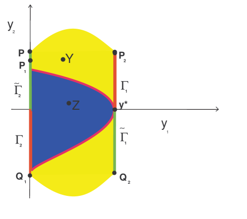
Figure 1: The region $G$ for system (3.14) is depicted in details. The curves of discontinuity $\Gamma=\Gamma_{1}\cup\Gamma_{2}$ and $\tilde{\Gamma}=\tilde{\Gamma}_{1}\cup\tilde{\Gamma}_{2}$ are drawn as vertical lines in red and green, respectively and the grazing orbit in magenta.

Define $\Gamma_{1}=\{(y_{1},y_{2})|\ y_{1}=\exp(0.00025\pi),\quad 0\leq y_{2}\leq y_{2}(\theta_{1},0,(0,\bar{y}_{2}))\},$ and $\Gamma_{2}=\{(y_{1},y_{2})|\ y_{1}=0,\,y_{2}(\theta_{2},0,-R_{1}y_{2}((\theta_{1},0,(0,\bar{y}_{2})))^{2})\leq y_{2}\leq 0\}.$ The boundary of the curve, $\Gamma=\Gamma_{1}\cup\Gamma_{2},$ has of four points, they are

$$\partial\Gamma=\{(0,0),(\exp(0.00025\pi),0),(\exp(0.00025\pi),y_{2}(\theta_{1},0,(0,\bar{y}_{2}))),(0,y_{2}(\theta_{2},0,-R_{1}y_{2}(\theta_{1},0,(0,\bar{y}_{2})))\}.$$

In the following part of the example, we will show that two of them, $y^{*}=(y_{1}^{*},y_{2}^{*})=(\exp(0.00025\pi),0)$ and the origin, $(0,0)$ are grazing points. Moreover, it can be easily validated that other two points are of $\beta-$type.

Issuing from system (3.14), the curve of discontinuity $\tilde{\Gamma}$ consists of two components $\tilde{\Gamma}_{1}$ and $\tilde{\Gamma}_{2}.$ The components are the following sets

$$\tilde{\Gamma}_{1}=\{(y_{1},y_{2})|\ y_{1}=\exp(0.00025\pi),\,-R_{1}y_{2}(\theta_{1},0,(0,\bar{y}_{2}))^{2}\leq y_{2}\leq 0\}$$

and

$$\tilde{\Gamma}_{2}=\{(y_{1},y_{2})|\ y_{1}=0,\,0\leq-R_{2}y_{2}(\theta_{2},0,Q_{2})\}.$$

One can verify that the function

$$\Psi(t)=\begin{cases}\exp(0.0005t)\Big{(}\sin(t),\cos(t)\Big{)},&\text{if }t\in[0,\pi),\\ (0,1),&\text{if }t=\pi,\end{cases}$$ (3.15)

is a discontinuous periodic solution of (3.14) with period $\omega=\pi,$ whose discontinuity points $(0,1)$ and $(0,-\exp(0.0005\pi))$ belong to $\tilde{\Gamma}$ and $\Gamma,$ respectively. The expression

$$\langle\nabla\Phi((\exp(0.00025\pi),0)),f((\exp(0.00025\pi),0))\rangle=\langle(1,0),(0,-\exp(-0.00025\pi))\rangle=0$$

verifies that $y^{*}$ is a $(\gamma)-$ type point, i.e. a grazing point of the solution $\Psi(t).$ It is easily seen that the grazing is axial. Now, we can assert that the periodic solution (3.15) is a grazing solution in the sense of Definition 2.5. Its simulation is depicted in Figure 2.

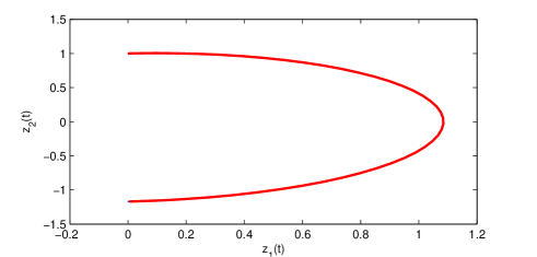
Figure 2: The grazing orbit of system (3.14).

Since the complement of $G$ is invariant in both directions and consists of continuous trajectories of the linear system (3.14a), one can easily conclude that the complement is a continuous dynamical system [23]. Thus, to verify the dynamics for the whole system, one need to analyze it in the region $G.$ This set is bounded, consequently for solutions in it conditions $(C8)$ and $(C9)$ are fulfilled and by Theorem 2.1, they admit $B-$sequences and continuation property.

Consider a function $\zeta(y_{2}):[y_{2}(\theta_{2},0,Q_{2}),y_{2}(\theta_{1},0,P)]\rightarrow[y_{2}(\theta_{2},0,Q_{2}),y_{2}(\theta_{1},0,P)]$ such that it is continuously differentiable, satisfies $\zeta(y_{2})=-R_{2}y_{2}$ in a neighborhood of $y_{2}=0$ and is the identity at the boundary points, i.e. $\zeta(y_{2}(\theta_{1},0,P))=y_{2}(\theta_{1},0,P)$ and $\zeta(y_{2}(\theta_{1},0,P))=y_{2}(\theta_{1},0,P).$ It is easily seen that such function exists. On the basis of this discussion, let us introduce the following system,

$$y_{1}^{\prime}=y_{2},$$ (3.16)

$$y_{2}^{\prime}=-y_{1}+0.001y_{2},$$

$${\Delta y_{2}|_{y\in\Gamma}}=\zeta(y_{2})-y_{2}.$$

It is apparent that system (3.16) is equivalent to (3.14) near the orbit of periodic solution $\Psi(t).$ That is, they have the same trajectories there.

Specifying (2.1) for (3.16), it is easy to obtain that $\Phi(y_{1},y_{2})=\tilde{\Phi}(y_{1},y_{2})=(y_{1}-\exp(0.00025\pi))y_{1},$ $f(y_{1},y_{2})=(y_{2},-y_{1}+0.001y_{2})$ and $J(y)=(y_{1},\zeta(y_{2})).$

Now, we will verify that system (3.16) defines a $K-$ smooth discontinuous flow. First, condition $(C1)$ is verified since $\nabla\Phi_{1}(y)=\nabla\Phi_{2}(y)=(1,0)\neq 0,$ for all $y\in D.$ The jump function $J(y)=(y_{1},\zeta(y_{2}))$ is continuously differentiable function. So, condition $(C2)$ is valid. It is true that $\Gamma\cap\tilde{\Gamma}\subseteq\partial\Gamma\cap\tilde{\partial\Gamma}.$ Inequalities $\langle\nabla\Phi_{1}(y),f(y)\rangle=\langle(1,0),(y_{2},-y_{1}+0.001y_{2})\rangle=y_{2}\neq 0$ and $\langle\nabla\Phi_{2}(y),f(y)\rangle=\langle(1,0),(y_{2},-y_{1}+0.001y_{2})\rangle=y_{2}\neq 0,$ if $y\in\Gamma\setminus\partial\Gamma,$ validate the condition $(C4).$ Moreover, $\langle\nabla\tilde{\Phi}_{1}(y),f(y)\rangle=\langle(1,0),(y_{2},-y_{1}+0.001y_{2})\rangle=y_{2}\neq 0$ and $\langle\nabla\tilde{\Phi}_{2}(y),f(y)\rangle=\langle(1,0),(y_{2},-y_{1}+0.001y_{2})\rangle=y_{2}\neq 0,$ if $y\in\tilde{\Gamma}\setminus\partial\tilde{\Gamma}.$ Conditions $(C6)$ and $(C7)$ hold as the function $\zeta$ is such defined. Thus, conditions $(C1)-(C10)$ have been verified. Consequently, the system (3.14) defines the $K-$ smooth discontinuous flow for all motions except the grazing ones. To complete the discussion, one need to linearize the system near the grazing solutions. First, we proceed with the linearization around the grazing periodic orbit (3.15).

The solution, $\Psi(t)$ has two discontinuity moments $\theta_{1}=\frac{\pi}{2}$ and $\theta_{2}=\omega$ in the interval $[0,\omega].$ The corresponding discontinuity points are of $(\gamma)-$ and $(\alpha)-$ types, respectively. Next, we will linearize the system at these points. The linearization at the second point exists [1] and the details of this will be analyzed in the next example. This time, we will focus on the grazing point $y^{*}.$

First, we assume that $y(t)=y(t,0,y^{*}+\Delta y),$ $\Delta y=(\Delta y_{1},\Delta y_{2})$ is not a grazing solution. Moreover, the solution intersects the line $\Gamma_{1}$ at time $t=\xi$ near $t=\theta_{1}$ as time increases. The meeting point $\bar{y}=(\bar{y}_{1},\bar{y}_{2})=(y_{1}(\xi,0,(y^{*}+\Delta y)),y_{2}(\xi,0,(y^{*}+\Delta y)),$ is transversal one. It is clear $\bar{y}_{1}=\exp(0.00025\pi)$ and $\bar{y}_{2}>0.$ In order to find a linearization at the moment $t=\theta_{i},$ we use formula (2.3) for $y(t),$ and find that

$$\displaystyle{\frac{\partial W_{i}(y)}{\partial y_{1}^{0}}} =\displaystyle{\int\limits_{\theta_{i}}^{\tau(y)}{\frac{\partial f(y(s))}{\partial y}\frac{\partial y(s)}{\partial y_{1}^{0}}ds}}+f(y(s))\frac{\partial\tau(y)}{\partial y_{1}^{0}}+J_{y}(y)(e_{1}+f(y(s))\frac{\partial\tau(y)}{\partial y_{1}^{0}})+f(y(s)+J(y(s)))\frac{\partial\tau(y)}{\partial y_{1}^{0}}$$ (3.17)

$$\displaystyle{+\int\limits_{\tau(y)}^{\theta_{i}}{\frac{\partial f(y(s)+J(y(s)))}{\partial x}\frac{\partial y(s)}{\partial y_{1}^{0}}ds}},$$

where $e_{1}=(1,0)^{T},$ $T$ denotes the transpose of a matrix. Substituting $y=\bar{y}$ to the formula (3.17), we obtain that

$$\displaystyle{\frac{\partial W_{i}(y(\xi,0,y^{*}+\Delta y))}{\partial y_{1}^{0}}=f(y(\xi,0,y^{*}+\Delta y))\frac{\partial\tau(y(\xi,0,y^{*}+\Delta y))}{\partial y_{1}^{0}}}$$

$$\displaystyle{+J_{y}(y(\xi,0,y^{*}+\Delta y))\Bigg{(}e_{1}+f(y(\xi,0,y^{*}+\Delta y)))\frac{\partial\tau(y(\xi,0,y^{*}+\Delta y)))}{\partial y_{1}^{0}}\Bigg{)}}$$

$$+\displaystyle{f(y(\xi,0,(J(y(\xi,0,y^{*}+\Delta y)))))\frac{\partial\tau(J(y(\xi,0,y^{*}+\Delta y)))}{\partial y_{1}^{0}}}.$$ (3.18)

Considering the formula (3.10) for the transversal point $\bar{y}=(\bar{y}_{1},\bar{y}_{2}),$ the first component $\displaystyle{\frac{\partial\tau(\bar{y})}{\partial y_{1}^{0}}}$ can be evaluated as $\displaystyle{\frac{\partial\tau(\bar{y})}{\partial y_{1}^{0}}=-\frac{1}{\bar{y}_{2}}}.$ From the last equality, it is seen how the singularity appears at the grazing point. Finally, we obtain that

$$\displaystyle{\frac{\partial W_{i}(\bar{y})}{\partial y_{1}^{0}}}=\begin{bmatrix}\bar{y}_{2}\\ -\bar{y}_{1}-0.001\bar{y}_{2}\end{bmatrix}\displaystyle{\Big{(}-\frac{1}{\bar{y}_{2}}\Big{)}}+\begin{bmatrix}1&0\\ 0&-2R_{1}\bar{y}_{2}\end{bmatrix}\Bigg{(}e_{1}+\begin{bmatrix}\bar{y}_{2}\\ -\bar{y}_{1}-0.001\bar{y}_{2}\end{bmatrix}\displaystyle{\Big{(}-\frac{1}{\bar{y}_{2}}\Big{)}}\Bigg{)}$$ (3.19)

$$-\begin{bmatrix}-R_{1}(\bar{y}_{2})^{2}\\ -\bar{y}_{1}+0.001R_{1}(\bar{y}_{2})^{2}\end{bmatrix}\displaystyle{\Big{(}-\frac{1}{\bar{y}_{2}}\Big{)}}=\begin{bmatrix}\bar{y}_{2}-R_{1}(\bar{y}_{2})^{2}\\ -\bar{y}_{1}-0.001(\bar{y}_{2}-R_{1}(\bar{y}_{2})^{2})\end{bmatrix}\displaystyle{\Big{(}-\frac{1}{\bar{y}_{2}}\Big{)}}+\begin{bmatrix}1&0\\ 0&-2R_{1}\bar{y}_{2}\end{bmatrix}\begin{bmatrix}0\\ \displaystyle{\frac{\bar{y}_{1}+0.001\bar{y}_{2}}{\bar{y}_{2}}}\end{bmatrix}.$$

Calculating the righthand side of (3.19) we have

$$\displaystyle{\frac{\partial W_{i}(\bar{y})}{\partial y_{1}^{0}}}=\begin{bmatrix}-R_{1}\bar{y}_{2}-1\\ 0.001(1-R_{1}\bar{y}_{2})+2R_{1}(0.001\bar{y}_{2}-\bar{y}_{1})\end{bmatrix}.$$ (3.20)

The last expression demonstrates that the derivative is a continuous function of its arguments in a neighborhood of the grazing point. Since it is defined and continuous for the points, which are not from the grazing orbit by the last expression and for other points it can be determined by the limit procedure. Indeed, one can easily show that the derivative at the grazing point $y^{*}$ is

$$\begin{bmatrix}-1\\ 0.001-1.8\exp(0.00025\pi)\end{bmatrix}.$$ (3.21)

Similarly, all other points of the grazing orbit can be discussed.

Next, differentiating (2.3) with $y(t)$ again we obtain that

$$\displaystyle{\frac{\partial W_{i}(y)}{\partial y_{2}^{0}}} =\displaystyle{\int\limits_{\theta_{i}}^{\tau(y)}{\frac{\partial f(y)}{\partial y}\frac{\partial y(s)}{\partial y_{2}^{0}}ds}}+f(y(s))\frac{\partial\tau(y)}{\partial y_{2}^{0}}+J_{y}(y)(e_{2}+f(y(s))\frac{\partial\tau(y)}{\partial y_{2}^{0}})+f(y+J(y))\frac{\partial\tau(y)}{\partial y_{2}^{0}}$$ (3.22)

$$\displaystyle{+\int\limits_{\tau(y)}^{\theta_{i}}{\frac{\partial f(y(s)+J(y(s)))}{\partial x}\frac{\partial y(s)}{\partial y_{2}^{0}}ds}},$$

where $e_{2}=(0,1)^{T}.$ Calculate the right hand side of (3.22) at the point $\bar{y}=(\bar{y}_{1},\bar{y}_{2})$ to obtain

$$\displaystyle{\frac{\partial W_{i}(y(\xi,0,y^{*}+\Delta y))}{\partial y_{2}^{0}}=f(y(\xi,0,y^{*}+\Delta y))\frac{\partial\tau(y(\xi,0,y^{*}+\Delta y))}{\partial y_{2}^{0}}}$$

$$\displaystyle{+J_{y}(y(\xi,0,y^{*}+\Delta y))\Bigg{(}e_{2}+f(y(\xi,0,y^{*}+\Delta y)))\frac{\partial\tau(y(\xi,0,y^{*}+\Delta y))}{\partial y_{2}^{0}}\Bigg{)}}$$

$$+\displaystyle{f(y(\xi,0,y^{*}+\Delta y))\frac{\partial\tau(y(\xi,0,y^{*}+\Delta y))}{\partial y_{2}^{0}}}.$$ (3.23)

To calculate the fraction $\displaystyle{\frac{\partial\tau(y(\xi,0,y^{*}+\Delta y))}{\partial y_{2}^{0}}}$ in (3.1), we apply formula (3.10) for the transversal point $\bar{y}=(\bar{y}_{1},\bar{y}_{2}).$ The second component $\displaystyle{\frac{\partial\tau(\bar{y})}{\partial y_{2}^{0}}}$ takes the form $\displaystyle{\frac{\partial\tau(\bar{y})}{\partial y_{2}^{0}}=0.}$ This and formula (3.1) imply

$$\displaystyle{\frac{\partial W_{i}(\bar{y})}{\partial y_{2}^{0}}}=\begin{bmatrix}0\\ -2R\bar{y}_{2}\end{bmatrix}.$$ (3.24)

Similar to (3.21), one can obtain that

$$\displaystyle{\frac{\partial W_{i}(y^{*})}{\partial y_{2}^{0}}}=\begin{bmatrix}0\\ 0\end{bmatrix}.$$ (3.25)

Joining (3.21) and (3.25), it can be obtained that

$$\displaystyle{W_{iy}(y^{*})}=\begin{bmatrix}-1&0\\ 0.001-1.8\exp(0.00025\pi)&0\end{bmatrix}.$$ (3.26)

The continuity of the derivatives in a neighborhood of $y^{*}$ implies that the function $W$ is differentiable at the grazing point $y=y^{*},$ and the condition $(A2)$ is valid.

Now, on the basis of the discussion made above, one can obtain the bivalued matrix of coefficients for the grazing point as

$$B_{1}=\begin{cases}O_{2},\ &\mbox{if (N1) is valid},\\ \begin{bmatrix}-1&0\\ 0.001-1.8\exp(0.00025\pi)&0\end{bmatrix},\ &\mbox{if (N2) is valid}.\end{cases}$$

The matrix $D_{1}^{(1)}=O_{2}$ is for near solutions of (3.15) which are in the region where $Z$ in, see Fig. 1, and do not intersect the curve of discontinuity $\Gamma_{1}.$ The matrix

$$D_{1}^{(2)}=\begin{bmatrix}-1&0\\ 0.001-1.8\exp(0.00025\pi)&0\end{bmatrix}$$

is for near solutions of (3.15), which intersects the curve of discontinuity $\Gamma_{1}.$ They start in the subregion, where the point $Y$ is placed. Thus, the linearization for $\Psi(t)$ at the grazing point exists. Moreover, since another point of discontinuity $(0,\exp(0.0005\pi))$ is not grazing, the linearization at the point exist as well as linearization at points of continuity [1, 40]. Consequently, there exist linearization around $\Psi(t).$

To verify condition $(A3),$ consider a near solution $y(t)=y(t,0,\bar{y})$ to $\Psi(t),$ where $\bar{y}=(0,\bar{y}_{2}),\,\bar{y}_{2}>\Psi_{2}(0)=1,$ which satisfy the condition $(N1).$ It is true that $\displaystyle{\theta_{i+1}-\theta_{i}=\frac{\pi}{2}=\frac{\omega}{2}.}$ The first coordinate of the near solution is $\displaystyle{y_{1}(t)=\bar{y}\exp(0.0005t)\sin(t)}$ and
$y_{1}(\frac{\omega}{2})=\displaystyle{y_{1}(\frac{\pi}{2})=\bar{y}\exp(0.00025\pi)}>\exp(0.00025\pi)=\Psi_{1}(\frac{\omega}{2}).$ Thus, the meeting moment of near solution $y(t)$ with the surface of discontinuity is less than $\frac{\omega}{2}.$ So, it implies that $0<\tau(y)<\frac{\pi}{2}-\epsilon$ for a small number $\epsilon$ if the first coordinate of $\bar{y}$ is close to $\exp(0.00025\pi).$ This validates condition $(A3).$ Now, Lemma 3.1 proves the condition $(C).$

Now, let us consider the point $(0,0).$ We have that $\langle\nabla\Phi((0,0)),f((0,0))\rangle=\langle(1,0),(0,0)\rangle=0.$ That is the origin is a grazing point. In the same time it is a fixed point of the system. For this particular grazing point, we can find the linearization directly. Indeed, all the near solutions satisfy the linear impulsive system,

$$x_{1}^{\prime}=x_{2},$$ (3.27)

$$x_{2}^{\prime}=-x_{1}+0.001x_{2},$$

$${\Delta x_{2}|_{x_{1}=0}=-(1+R_{2})x_{2}.}$$

Consider a solution $x(t)=x(t,0,x_{0}),$ where $x_{0}=(x_{1}^{0},x_{2}^{0})\not=(0,0)$ with moments of discontinuity $\theta_{i},i\in\mathbb{Z},$ then the linearization system for the equation around the equilibrium is

$$u_{1}^{\prime}=u_{2},$$ (3.28)

$$u_{2}^{\prime}=-u_{1}+0.001u_{2},$$

$${\Delta u_{2}|_{t=\theta_{i}}=-(1+R_{2})u_{2}.}$$

Indeed, if $u_{1}(t),$ $u_{1}(0)=e_{1},$ $u_{2}(t),$ $u_{2}(0)=e_{2},$ are solutions of (3.28), then one can see that $x(t)-(0,0)=x_{1}^{0}u_{1}(t)+x_{2}^{0}u_{2}(t),$ for all $t\in\mathbb{R}.$

We have obtained that linearization exists for both grazing solutions $\Psi(t),$ and the equilibrium at the origin. Moreover, conditions $(C1)-(C10)$ are valid and all other solutions are B-differentiable in parameters [1]. Thus, the system (3.14) defines a $K-$ smooth discontinuous flow in the plane.

In the next example, we will finalize the linearization around the grazing solution $\Psi(t).$

Example 3.2

(Linearization around the grazing discontinuous cycle). We continue analysis of the last example, and complete the variational system for $\Psi(t).$

Let us consider this time, the linearization at the non-grazing moment $\omega=\pi.$ The discontinuity point is $c=(0,-\exp(0.0005\pi))$ and it is of $(\alpha)-$ type, since

$$\langle\nabla\Phi(c),f(c)\rangle=\langle(1,0)(-\exp(0.0005\pi),-0.001\exp(0.0005\pi))\rangle=-\exp(0.0005\pi)\neq 0.$$

By using formula (3.10), one can compute the gradient as $\displaystyle{\nabla\tau(c)=(\exp(-0.0005\pi),0)}.$

Then, utilizing $\nabla\tau(c)$ and formula (3.11), one can determine that the matrix of linearization at the moment $\pi$ is

$$B_{2}=\begin{bmatrix}\exp(-0.0005\pi)&0\\ 0.001&0\end{bmatrix}.$$

From the monotonicity of the jump function, $-R_{1}y_{2}^{2},$ it follows that the the yellow and blue subregions of $G$ are invariant. Consequently, for each solution near to $\Psi(t),$ the sequences $B_{i}$ is of two types $B_{i}=D_{i}^{(j)},$ $i\in\mathbb{Z}$ and $j=1,2,$ where $D_{2i-1}^{(1)}=O_{2},$ $D_{2i-1}^{(2)}=D_{1}^{(2)}=\begin{bmatrix}-1&0\\ 0.001-1.8\exp(0.00025\pi)&0\end{bmatrix},$ $D_{2i}^{(1)}=D_{2i}^{(2)}=\begin{bmatrix}\exp(-0.0005\pi)&0\\ 0.001&0\end{bmatrix},i\in\mathbb{Z}.$ That is, the condition $(A4)$ is valid and the linearization around the periodic solution (3.15) on $\mathbb{R}$ is of two subsystems:

$$u_{1}^{\prime}=u_{2},$$ (3.29)

$$u_{2}^{\prime}=-u_{1}+0.001u_{2},$$

$$\Delta u|_{t=\theta_{2i-1}}=D_{2i-1}^{(1)}u,$$

$$\Delta u|_{t=\theta_{2i}}=D_{2i}^{(1)}u,$$

and

$$u_{1}^{\prime}=u_{2},$$ (3.30)

$$u_{2}^{\prime}=-u_{1}+0.001u_{2},$$

$$\Delta u|_{t=\theta_{2i-1}}=D_{2i-1}^{(2)}u,$$

$$\Delta u|_{t=\theta_{2i}}=D_{2i}^{(2)}u,$$

where $\theta_{2i-1}=\frac{(2i-1)\pi}{2}$ and $\theta_{2i}=i\pi$

The sequences $\{D_{i}^{(j)}\},\ j=1,2,$ are $2-$ periodic. It is appearant that system (3.29)+(3.30) is a $(\omega,2)-$ periodic. Thus, the variational system for the grazing solution is constructed.

4 Orbital stability

In this section, we proceed investigation of the grazing periodic solution $\Psi(t).$ Analysis of orbital stability will be taken into account. Denote by $B(z,\delta),$ an open ball with center at $z$ and the radius $\delta>0$ for a fixed point $z\in\Gamma\setminus\partial\Gamma.$ By condition (C3), the ball is divided by surface $\Gamma$ into two connected open regions. Denote $c^{+}(z,\delta),$ for the region, where solution $x(t)=x(t,0,z)$ of (2.2) enters as time increases. The region is depicted in Figure 3.

Set the path of the periodic solution $\Psi(t)$ as

$$\eta:=\{x\in D:x=\Psi(t),\quad t\in\mathbb{R}\}.$$

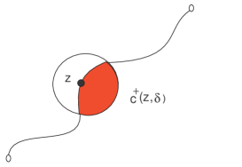
Figure 3: The region $c^{+}(z,\delta).$

Define $dist(A,a)=\inf_{\alpha\in A}\|\alpha-a\|,$ where $A$ is a set, and $a$ is a point.

Definition 4.1

The periodic solution $\Psi(t):\mathbb{R}\rightarrow D$ of (2.1) is said to be orbitally stable if for every $\epsilon>0,$ there corresponds $\delta=\delta(\epsilon)>0$ such that $dist(x(t,0,x_{0}),\eta)<\epsilon,$ for all $t\geq 0,$ provided $dist(x_{0},\eta)<\delta$ and $x_{0}\notin\cup_{i}c^{+}(\Psi(\theta_{i}),\delta),\ for\ i=1,\ldots,m,$ where $m$ is the number of points $\Psi(\theta_{i})\in\Gamma\setminus\partial\Gamma.$

The point $x_{0}$ is not considered in regions $c^{+}(\Psi(\theta_{i}),\delta),i=1,\ldots,m,$ since solutions which start there move continuously on a finite interval, while $\Psi(t)$ experiences a non-zero jump at $t=\theta_{i}$ and this violates the continuity in initial value, in general. In the same time, we take into account any region adjoint to points of $\partial\Gamma,$ since the jump of $\Psi(t)$ is zero there and, consequently, the continuous dependence in initial value is valid for all near points.

Definition 4.2

The solution $\Psi(t):\mathbb{R_{+}}\rightarrow D$ of (2.1) is said to have asymptotic phase property if a $\delta>0$ exists such that to each $x_{0}$ satisfying $dist(x_{0},\eta)<\delta$ and $x_{0}\notin\cup_{i}c^{+}(\Psi(\theta_{i}),\delta),\ for\ i=1,\ldots,m,$ there corresponds an asymptotic phase $\alpha(x_{0})\in\mathbb{R}$ with property: for all $\epsilon>0,$ there exists $T(\epsilon)>0,$ such that $x(t+\alpha(x_{0}),0,x_{0})$ is in $\epsilon$-neighborhood of $\Psi(t)$ in $B-$topology for $t\in[T(\epsilon),\infty).$

Let us consider the following system, which will be needed in the following lemmas and theorem

$$x^{\prime}=A(t)x,$$ (4.31)

$$\Delta x|_{t=\zeta_{i}}=B_{i}u,$$

where $A(t)$ and $B_{i}$ are $n\times n$ function-matrices, $A(t+\omega)=A(t),$ for all $t\in\mathbb{R}$ and there exists an integer $p$ such that $\zeta_{i+p}=\zeta_{i}+\omega$ and $B_{i+p}=B_{i},$ for all $i\in\mathbb{Z}.$

Lemma 4.1

Assume that system (4.31) has a simple unit characteristic multiplier and the remaining $n-1$ ones are in modulus less than unity. Then, the system (4.31) has a real fundamental matrix $X(t),$ of the form

$$X(t)=P(t)\left(\begin{array}[]{cc}1&0\\ 0&\exp{(Bt)}\end{array}\right),$$ (4.32)

where $P\in PC^{1}(\mathbb{R},\theta)$ is a regular, $\omega$-periodic matrix, and $B$ is an $(n-1)\times(n-1)$ matrix with all eigenvalues have negative real parts.

Proof. Denote the matrix $X(t),X(0)=I,$ as fundamental matrix of system (4.31). There exists a matrix $B_{1}$ such that the substitution $x=P(t)z,$ where $P(t)=X(t)\exp(-B_{1}t),$ transforms (4.31) to the following system with constant coefficient [1],

$$z^{\prime}=\Lambda z.$$ (4.33)

The matrix $\exp(\Lambda\omega)$ has a simple unit eigenvalue and remaining $(n-1)$ ones are in modulus less than unity. Hence, there exists real nonsingular matrix $M,$ which satisfies

$$M^{-1}\exp(\Lambda\omega)M=\begin{bmatrix}1&0\\[3.00003pt] 0&C_{1}\\[3.00003pt] \end{bmatrix}.$$

The remaining part of the proof is same as proof of Lemma 5.1.1 in [17]. $\square$

Throughout this section, we will assume that $(A4)$ is valid. That is, the variational system (3.13) consists of $m$ periodic subsystems. For each of these systems, we find the matrix of monodromy, $U_{j}(\omega)$ and denote corresponding Floquet multipliers by $\rho_{i}^{(j)},$ $i=1,\ldots,n,$ $j=1,\ldots,m.$ In the next part of the paper, the following assumption is needed.

• $\rho_{1}^{(j)}=1$ and $|\rho_{i}^{(j)}|<1,$ $i=2,\ldots,n$ for each $j=1,\ldots,m.$

Lemma 4.2

Assume that the assumptions (A4) and (A5) are valid. Then, for each $j=1,\ldots,m,$ the system (3.13) admits a fundamental matrix of the form

$$U_{j}(t)=P_{j}(t)[1,\exp(H_{j}\omega)],\quad t\in\mathbb{R},$$ (4.34)

where $P_{j}\in PC^{1}(\mathbb{R},\zeta)$ is a regular, $\omega$-periodic matrix and $H_{j}$ is an $(n-1)\times(n-1)-$ matrix with all eigenvalues have negative real parts.

The proof of Lemma 4.2, can be done similar to that of Lemma 4.1.

Theorem 4.1

Assume that conditions $(C1)-(C7),$ $(C10),$ and the assumptions $(A1)-(A5)$ hold. Then $\omega$- periodic solution $\Psi(t)$ of $(\ref{eq:graz1})$ is orbitally asymptotically stable and has the asymptotic phase property.

Proof. Since of the group property, we may assume $\Psi(0)$ is not a discontinuity point. Then, one can displace the origin to the point $\Psi(0),$ and the coordinate system can be rotated in such a way that the tangent vector $\Psi^{\prime}_{0}=\Psi^{\prime}(0)$ points in the direction of the positive $x_{1}$ axis i.e. the coordinates of this vector are $\Psi^{\prime}_{0}=(\Psi^{\prime}_{01},0,\ldots,0),$ $\Psi^{\prime}_{01}>0.$

Let $\theta_{i},i\in\mathbb{Z},$ be the discontinuity moments of $\Psi(t).$ Denote the path of the solution by $\eta=\{x\in X:x=\Psi(t),t\in\mathbb{R}\}.$ There exists a natural number $p,$ such that $\theta_{i+p}=\theta_{i}+\omega$ for all $i.$ Because of conditions $(C1)-(C7)$ and $K-$differentiability of $\Psi(t)$ there exists continuous dependence on initial data and consequently there exists a neighborhood of $\eta$ such that any solutions which starts in the set will have moments of discontinuity which constitute a $B-$ sequence with difference between neighbors approximately equal to the distance between corresponding neighbor moments of discontinuity of the periodic solution $\Psi(t).$ Consequently we can determine variational system for $\Psi(t),$ with points of discontinuity $\theta_{i},\ i\in\mathbb{Z}.$

On the basis of discussion in Section $2.1,$ one can define in the neighborhood of $\eta$ a $B-$ equivalent system of type (2.4). The variational system of it takes the form

$$z^{\prime}=A(t)z+r(t,z),$$ (4.35)

$${\Delta z|_{t=\theta_{i}}}=D_{i}^{(j)}z+q_{i}(z),\quad j=1,2,\ldots,m,$$

where $r(t,z)=[f(\Psi(t)+z)-f(\Psi(t))]-A(t)z$ and $q_{i}(z)=W_{i}(\Psi(\theta_{i})+z)-W_{i}(\Psi(\theta_{i}))-D_{i}^{(j)}z,$ are continuous functions, and matrices $D_{i}^{(j)}$ satisfy condition $(A4).$ The functions are continuously differentiable with respect to $z.$ One can verify that $r(t,0)\equiv q_{i}(0)\equiv 0$ and $r(t+\omega,z)=r(t,z)$ for $t\in\mathbb{R}.$ Moreover, the derivatives satisfy $r^{\prime}(t,0)\equiv q_{iz}^{\prime}(0)\equiv 0$ and the functions $r(t,z)\rightarrow 0,$ $q_{i}(z)\rightarrow 0,$ $r^{\prime}_{z}(t,z)\rightarrow 0$ and $q_{iz}^{\prime}(z)\rightarrow 0,$ as $z\rightarrow 0$ uniformly in $t\in[0,\infty),\ i\geq 0.$ Each system (4.35) for $j=1,2,\ldots,m,$ corresponds to a region adjoint to initial value, $x_{0}$ such that these regions cover a neighborhood of $x_{0}.$

Fix a number $j$ and denote $Y_{j}(t)$ the fundamental matrix of adjoint to (4.35) linear homogeneous system

$$y^{\prime}=A(t)y,$$ (4.36)

$${\Delta y|_{t=\theta_{i}}}=D_{i}^{(j)}y,$$

of the form (4.34). One can verify that

$$Y_{j}(t)Y_{j}^{-1}(s)=P_{j}(t)\left(\begin{array}[]{cc}1&0\\ 0&\exp(H_{j}(t-s))\end{array}\right)P_{j}^{-1}(s),$$ (4.37)

for $-\infty<t,s<\infty.$

We can write

$$\left(\begin{array}[]{cc}1&0\\ 0&\exp(H_{j}(t-s))\end{array}\right)=\left(\begin{array}[]{cc}0&0\\ 0&\exp(H_{j}(t-s))\end{array}\right)+\left(\begin{array}[]{cc}1&0\\ 0&O_{n-1}\end{array}\right),$$

where $O_{n-1}$ is the $(n-1)\times(n-1)$ zero matrix. Then it can be driven

$$Y_{j}(t)Y_{j}^{-1}(s)=G_{1}^{(j)}(t,s)+G_{2}^{(j)}(t,s)=G^{(j)}(t,s),$$

where

$$G_{1}^{(j)}(t,s)=P_{j}(t)\left(\begin{array}[]{cc}0&0\\ 0&\exp(H_{j}(t-s))\end{array}\right)P_{j}^{-1}(s),$$

$$G_{2}^{(j)}(t,s)=P_{j}(t)\left(\begin{array}[]{cc}1&0\\ 0&O_{n-1}\end{array}\right)P_{j}^{-1}(s).$$

Denote the eigenvalues of the matrix $H_{j}$ by $\lambda_{2}^{(j)},\ldots,\lambda_{n}^{(j)}.$ By means of the Lemma 4.1 and 4.2, there exits a number $\alpha>0,$ such that $Re(\lambda_{k}^{(j)})<-\alpha,$ $k=2,3,\ldots,n,$ where $Re(z)$ means the real part of the number, $z.$ Taking into account that the matrices $P_{j}$ and $P_{j}^{-1}$ are regular and periodic, the following estimates can be calculated

$$|G_{1}^{(j)}(t,s)|\leq K^{(j)}\exp(-\alpha(t-s)),$$ (4.41)

$$|G_{2}^{(j)}(t,s)|\leq K^{(j)},$$ (4.42)

where $K^{(j)}$ is a positive real constant.

Denote the first column of the fundamental matrix $Y$ by $\chi^{1}.$ By the equation (4.34), $\chi^{1}$ is equal to the first column of $P_{j},$ this means that it is a $\omega$-periodic solution of (3.13).

By assumptions of the theorem the variational system (4.35) satisfies the conditions of Lemma 4.2, and one can verify that the following estimate is true [17]

$$|Y_{j}(t)|\leq K_{1}^{(j)}\exp(-\alpha t)\ \ for\ \ t\geq 0,$$ (4.43)

where $K_{1}^{(j)}$ is a positive constant. Let us setup the following integral equation

$$z^{(j)}(t,a)=Y_{j}(t)a+\int\limits^{t}_{0}{G_{1}^{(j)}(t,s)r(s,z(s))ds}-\int\limits^{\infty}_{t}{G_{2}^{(j)}(t,s)r(s,z(s))ds}$$

$$+\sum\limits_{0<\theta_{k}<t}{G_{1}^{(j)}(t,\theta_{k}+)q_{k}(z(\theta_{k}))}-\sum\limits_{t<\theta_{k}<\infty}{G_{2}^{(j)}(t,\theta_{k}+)q_{k}(z(\theta_{k}))},$$ (4.44)

where $a=[0,a_{2},\ldots,a_{n}],$ $a_{i}\in\mathbb{R},$ $i=2,3,\ldots,n,$ are orthogonal to $\Psi^{\prime}(0),$ i.e. with the zero first coordinate.

Let $z_{0}^{(j)}(t,a)\equiv 0,$ and consider the following successive approximations

$$z_{k}^{(j)}(t,a)=Y_{j}(t)a+\int\limits^{\infty}_{0}{G^{(j)}(t,s)r(s,z_{k-1}(s))ds}+\sum\limits^{\infty}_{k=1}{G^{(j)}(t,\theta_{k}+)q_{k}(z_{k-1}(\theta_{k}))},$$ (4.45)

for $k=1,2,\ldots.$ By using the approximation (4.45) and estimation (4.43), one can verify that

$$|z_{1}^{(j)}(t,a)|\leq K_{1}^{(j)}|a|\exp(-\alpha t/2).$$ (4.46)

We will show that the bounded solution of (4) exists and satisfies (4.35). For arbitrary positive small number $L$, there exists a number $\delta=\delta(L)$ such that for $|z_{1}|<\delta,$ $|z_{2}|<\delta$

$$|r(t,z_{1})-r(t,z_{2})|\leq L|z_{1}-z_{2}|$$ (4.47)

and

$$|q_{i}(z_{1})-q_{i}(z_{2})|\leq L|z_{1}-z_{2}|,$$ (4.48)

uniformly in $t\in[0,\infty).$

Denote by $\displaystyle{L_{1}=4K^{(j)}\Big{(}\frac{2}{\alpha}-\frac{1}{1-\exp(-\alpha\underline{\theta}/2)}\Big{)}}.$

Next, by using mathematical induction, we are going to show that $z_{s}^{(j)}(t,a),s=1,2,\ldots,$ are defined for $t\in[0,\infty)$ and satisfy

$$|z_{s+1}^{(j)}(t,a)-z_{s}^{(j)}(t,a)|\leq K_{1}^{(j)}|a|\exp(-\alpha t/2)/2^{s},\,s=0,1,2,\ldots,$$ (4.49)

if $L<L_{1}.$ Utilizing Lemma 4.2 and inequalities (4.43), (4.47), (4.48) and $\theta_{i+1}-\theta_{i}\geq\underline{\theta},i\in\mathbb{Z},$ one can verify that

$$|z_{k+1}^{(j)}(t,a)-z_{k}^{(j)}(t,a)|\leq K_{1}^{(j)}|a|L_{1}\exp(-\alpha t/2)/(2^{k}\alpha).$$ (4.50)

As a consequence of (4.49), the sequence $z_{k+1}^{(j)}(t,a)$ converges uniformly on $t\in[0,\infty),\ |a|<\delta/2K_{1}^{(j)},$ and

$$|z_{s}^{(j)}(t,a)|\leq 2K_{1}^{(j)}|a|\exp(-\alpha t/2),s=1,2,\ldots.$$

Therefore, the limit function $z^{(j)}(t,a)$ exists on the same domain, it is piecewise continuous, satisfies (4) and the following estimate

$$|z^{(j)}(t,a)|\leq 2K_{1}^{(j)}|a|\exp(-\alpha t/2).$$ (4.51)

Denote by $z(t)=z^{(j)}(t,a),$ for $j=1,2,\ldots,m.$ Next, we will verify that $z^{(j)}(t,a)$ satisfies (4.35). For it, differentiate (4)

$$z^{\prime}(t)=Y^{\prime}_{j}(t)a+G_{1}^{(j)}(t,t)r(t,z(t))+G_{2}^{j}(t,t)r(t,z(t))+\int\limits^{t}_{0}{G_{1t}^{(j)}(t,s)r(s,z(s))ds}$$

$$-\int\limits^{\infty}_{t}{G_{2t}^{(j)}(t,s)r(s,z(s))ds}+\sum\limits_{0<\theta_{k}<t}{G_{1t}^{(j)}(t,\theta_{k}+)q_{k}(z(\theta_{k}))}-\sum\limits_{t<\theta_{k}<\infty}{G_{2t}^{(j)}(t,\theta_{k}+)q_{k}(z(\theta_{k}))}$$

$$=A(t)Y_{j}(t)a+G^{(j)}(t,t)r(t,z(t))+\int\limits^{\infty}_{0}{A(t)G^{(j)}(t,s)r(s,z(s))ds}+\sum\limits_{0<\theta_{i}<t}{A(t)G^{(j)}(t,\theta_{k}+)q_{k}(z(\theta_{k}))}$$

$$=A(t)z(t)+r(t,z(t)).$$

Fix $\theta_{k},$ $k\in\mathbb{Z},$ then

$$z(\theta_{k}+)-z(\theta_{k}) =Y_{j}(\theta_{k}+)a+\int\limits^{\theta_{k}}_{0}{G_{1}^{(j)}(\theta_{k}+,s)r(s,z(s))ds}-\int\limits^{\infty}_{\theta_{k}}{G_{2}^{(j)}(\theta_{k}+,s)r(s,z(s))ds}$$

$$+\sum\limits_{0\leq\theta_{i}<\theta_{k}}{G_{1}^{(j)}(\theta_{k}+,\theta_{i}+)q_{i}(z(\theta_{i}+))}-\sum\limits_{\theta_{k}<\theta_{i}<\infty}{G_{2}^{(j)}(\theta_{k}+,\theta_{i}+)q_{i}(z(\theta_{i}+))}$$

$$-Y_{j}(\theta_{k})a-\int\limits^{\theta_{k}}_{0}{G_{1}^{(j)}(\theta_{k},s)r(s,z(s))ds}+\int\limits^{\infty}_{\theta_{k}}{G_{2}^{(j)}(\theta_{k},s)r(s,z(s))ds}$$

$$-\sum\limits_{0\leq\theta_{i}<\theta_{k}}{G_{1}^{(j)}(\theta_{k},\theta_{i}+)q_{i}(z(\theta_{i}))}+\sum\limits_{\theta_{k}\leq\theta_{i}<\infty}{G_{2}^{(j)}(\theta_{k},\theta_{i}+)q_{i}(z(\theta_{i}+))}$$

$$=D_{k}^{(j)}z(\theta_{k})+q_{k}(z(\theta_{k})).$$

The above discussion proves that $z^{(j)}(t,a),j=1,,2,\ldots,m,$ are bounded solutions of system (4.35).

We will determine the initial values of bounded solutions in terms of $(n-1)$ parameters $a_{2}^{(j)},\ldots,a_{n}^{(j)},j=1,,2,\ldots,m.$ Denote $a^{(j)}=[0,a_{2}^{j},a_{3}^{j},\ldots,a_{n}^{j}].$ By using (4), we obtain

$$z^{(j)}(0,a^{(j)}) =Y_{j}(0)a^{(j)}-\int\limits^{\infty}_{0}{G_{2}^{(j)}(0,s)r(s,z(s))ds}-\sum\limits_{0<\theta_{k}<\infty}{G_{2}^{(j)}(0,\theta_{k}+)q_{k}(z(\theta_{k}))}$$

$$=P_{j}(0)a^{(j)}-P_{j}(0)\left(\begin{array}[]{cc}1&0\\ 0&O_{n-1}\end{array}\right)\int\limits^{\infty}_{0}{P_{j}^{-1}(s)r(s,z(s))ds}-\sum\limits_{0<\theta_{k}<\infty}{P_{j}^{-1}(s)q_{k}(z(\theta_{k}))}.$$

In the way utilized in [17], one can show that the coordinates of the initial value $(x_{1},\ldots,x_{n})\in D$ of the solution $z^{(j)}$ satisfy the equation

$$x_{1}+\sum\limits_{i=2}^{n}{c_{i}^{j}x_{i}-h_{j}(x_{2},\ldots,x_{n})=0},$$ (4.53)

where $h_{j}\in C^{1},j=1,,2,\ldots,m.$

One can see that equation (4.53) determines $(n-1)$ dimensional hypersurfaces $S^{j}\subset D,$ $j=1,2,\ldots,m,$ in a neighborhood of the origin such that each solution which starts at the surface satisfies inequality (4.51). From the analytical representation, it follows that the equation of the tangent space of $S^{j}$ at the origin is described by the equation $x_{1}+\sum\limits_{i=2}^{n}{c_{i}^{j}x_{i}}$ and the first coordinate of the gradient of the left hand side in (4.53) is unity. Moreover, the path $\eta$ intersects $S^{j}$ transversely. This and condition $(A4)$ imply that the path of every solution $\phi(t)$ near $\Psi(t)$ intersects one of the manifolds $S^{j},j=1,2,\ldots,m,$ at some $\bar{t}\in[0,2\omega].$

Because of the continuous dependence on initial values, a $\delta(\epsilon)>0$ exists for a given $\epsilon>0,$ such that if $dist(x^{0},\eta_{\delta})<\delta(\epsilon),$ then the solution $\phi(t,x^{0})$ is defined on $[0,2\omega],$ and $dist(\phi(t,x^{0}),\eta)<\epsilon\leq\epsilon_{1}$ for $t\in[0,2T].$ Therefore, the path of $\phi(t,x^{0})$ intersects $S^{j}$ for some $j=1,2,\ldots,m$ and $t_{1}\in[0,2\omega].$ The solution $\phi(t,\phi(t_{1},x^{0}))=\phi(t+t_{1},x^{0})$ has its initial value in $S^{j},$ consequently, satisfies (4.51). In the light of the $B-$ equivalence, the corresponding solution $x(t),x(0)=\phi(0)-\Psi(0),$ of (4.35) satisfies the property that for all $\epsilon>0,$ there exists $T(\epsilon)$ such that $x(t)$ is in an $\epsilon-$ neighborhood of $\Psi(t)$ for $t\in[T(\epsilon),\infty).$ That is, the solution $\Psi(t)$ is orbitally asymptotically stable and there exists an asymptotical phase. $\square$

Definitions of the orbital stability and an asymptotic phase as well as theorem of orbital stability for non-grazing periodic solutions are also presented in [44]. In our paper, we suggest the orbital stability theorem for grazing periodic solutions, its proof and formulate the definitions for the stability. They are different in many aspects from those provided in [44]. It is valuable that they also valid, if the solution is non-grazing.

To shed light on our theoretical results, we will present the following examples.

Example 4.1

We continue with the system presented in Examples 3.1 and 3.2. In Example 3.1, we verified that system (3.16)defines a $K-$ smooth discontinuous flow in the plane and the variational system (3.29)+(3.30) around the grazing periodic solution, $\Psi(t)$ is approved.

Using systems (3.29) and (3.30), one can evaluate the Floquet multipliers as $\rho_{1}^{(1)}=1,$ $\rho_{2}^{(1)}=0.8551,$ $\rho_{1}^{(2)}=1$ and $\rho_{2}^{(2)}=0.$ This verifies condition $(A5).$

The conditions $(C1)-(C7)$ and $(C10)$ are validated and the assumptions (A4) and (A5) verified. By using Theorem 4.1, we can assert that the solution, $\Psi(t)$ is orbitally asymptotically stable. The stability is illustrated in Fig. 4. The red one is for a trajectory of the discontinuous periodic solution (3.15) of (3.14) and the blue one is for the near solution of (3.14) with initial value $y_{0}=(0.8,1.2).$ It can be observed from Fig. 4 that the blue trajectory approaches the red one as time increases.

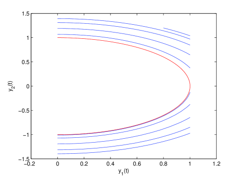
Figure 4: The red discontinuous cycle of (3.14) axially grazes $\Gamma$ at $(0.00025\pi),0)$ and $(0,-\exp(-0.0005\pi))$ is an $(\alpha)$-type point. The blue arcs are of the trajectory with initial value $(0.8,1.2).$ It can be observed that it approaches the grazing one as time increases.

Example 4.2

(A periodic solution with a non-axial grazing). We will take into account the following autonomous system with variable moments of impulses

$$x_{1}^{\prime}=x_{2},$$ (4.54)

$$x_{2}^{\prime}=-x_{1},$$

$${\Delta x_{1}|_{x\in\Gamma}=\frac{1}{\sqrt{2}}-x_{1}+K(x_{2}-x_{1})^{2},}$$

$${\Delta x_{2}|_{x\in\Gamma}=\frac{1}{\sqrt{2}}-x_{2}+K(x_{2}-x_{1})^{2},}$$

where $\Gamma=\{(x_{1},x_{2})|x_{1}+x_{2}=\sqrt{2}\},$ $\tilde{\Gamma}=\{(x_{1},x_{2})|x_{1}=x_{2}\}$ and $K=0.11.$ It is easy to verify that the point $\displaystyle{x^{*}=(\frac{1}{2},\frac{1}{2})}$ is a grazing point because $\langle\nabla\tau(x^{*}),f(x^{*})\rangle=\langle(1,1),(\frac{1}{2},-\frac{1}{2})\rangle=0$ and the grazing is non-axial. We assume that the domain is the plane.

The solution $\Psi(t)=(\sin(t),\cos(t)),$ $t\in\mathbb{R}$ is a grazing one, since the point $x^{*}=\Psi(\frac{\pi}{4})$ is from its orbit. The cycle and the line of discontinuity are depicted in Figure 5.

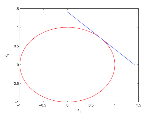
Figure 5: The red curve is the orbit of $\Psi(t)$ which grazes non-axially the line of discontinuity.

Let us consider the linearization at the grazing point $x^{*}$ next. We will consider the near solution $x(t)=x(t,0,x^{*}+\Delta x).$ Denote $t=\xi,$ the moment when the solution meets the surface of discontinuity $\Gamma$ at the point $\bar{x}=x(\xi)=x(\xi,0,x^{*}+\Delta x).$ Taking into account formulae (3.17), (3.1) with (4.54), one can obtain the following matrix

$$\displaystyle{\frac{\partial W_{i}(x(\xi,0,x^{*}+\Delta x))}{\partial x_{1}^{0}}}=\begin{bmatrix}\bar{x}_{2}\\ -\bar{x}_{1}\end{bmatrix}\frac{1}{\bar{x}_{1}-\bar{x}_{2}}\displaystyle{+\begin{bmatrix}-2K(\bar{x}_{2}-\bar{x}_{1})&-2K(\bar{x}_{2}-\bar{x}_{1})\\ -2K(\bar{x}_{2}-\bar{x}_{1})&-2K(\bar{x}_{2}-\bar{x}_{1})\end{bmatrix}}$$

$$\times\Bigg{(}e_{1}+\begin{bmatrix}\bar{x}_{2}\\ -\bar{x}_{1}\end{bmatrix}\frac{1}{\bar{x}_{1}-\bar{x}_{2}}\Bigg{)}+\displaystyle{\begin{bmatrix}-\frac{1}{\sqrt{2}}+K(\bar{x}_{2}-\bar{x}_{1})^{2}\\ \frac{1}{\sqrt{2}}-K(\bar{x}_{2}-\bar{x}_{1})^{2}\end{bmatrix}\frac{1}{\bar{x}_{1}-\bar{x}_{2}}}.$$ (4.55)

Calculating the right hand side of the expression (4.2), we obtain that

$$\displaystyle{\frac{\partial W_{i}(x(\xi,0,x^{*}+\Delta x))}{\partial x_{1}^{0}}}=\begin{bmatrix}\displaystyle{\frac{-\sqrt{2}+0.22}{2\sqrt{2}}}\\[6.0pt] \displaystyle{\frac{\sqrt{2}+0.22}{2\sqrt{2}}}\end{bmatrix}.$$ (4.56)

Using similar method with that of the first one, the second derivative can be computed as

$$\displaystyle{\frac{\partial W_{i}(x(\xi,0,x^{*}+\Delta x))}{\partial x_{2}^{0}}}=\begin{bmatrix}\displaystyle{\frac{\sqrt{2}+0.22}{2\sqrt{2}}}\\[6.0pt] \displaystyle{\frac{-\sqrt{2}+0.22}{2\sqrt{2}}}\end{bmatrix}.$$ (4.57)

Combining (4.56) and (4.57), we can obtain the following matrix for the linearization at the grazing point $x^{*},$

$$\displaystyle{W_{ix}(x^{*})}=\displaystyle{\begin{bmatrix}\displaystyle{\frac{-\sqrt{2}+0.22}{2\sqrt{2}}}&\displaystyle{\frac{\sqrt{2}+0.22}{2\sqrt{2}}}\\ \displaystyle{\frac{\sqrt{2}+0.22}{2\sqrt{2}}}&\displaystyle{\frac{-\sqrt{2}+0.22}{2\sqrt{2}}}\end{bmatrix}.}$$ (4.58)

It is appearant that the matrix $W_{ix}(x^{*})$ is continuous with respect to its arguments, since it is constant if the point $x^{*}+\Delta x$ is not from the orbit of the grazing solution. Since of the limit procedure, it is the same constant for all points of the grazing solution. Thus, the Jacobian is constant matrix in a neighborhood of the grazing point and condition $(A2)$ is valid.

Now, let us check the validity of the condition $(A3).$ Consider a near solution $x(t)=x(t,0,\bar{x}),$ to the grazing cycle $\Psi(t),$ where $\bar{x}=(0,\bar{x}_{2}),\,\bar{x}_{2}>\Psi_{2}(0)=1.$ So, the near solution $x(t)$ satisfies the condition $(N1).$ For the grazing periodic solution, it is true that $\theta_{i+1}-\theta_{i}=2\pi=\omega.$ The grazing solution $\Psi(t)=x(t,0,(0,1)),$ touches the line of discontinuity $\Gamma$ at $t=\frac{\omega}{8}.$ The first coordinate of the near solution is $x_{1}(t)=\bar{x}_{2}\sin(t),$ and $\displaystyle{x_{1}(\frac{\omega}{8})=\bar{x}_{2}\sin(\frac{\omega}{8})=\frac{\bar{x}_{2}}{\sqrt{2}}>\Psi_{1}(\frac{\omega}{8})=\frac{1}{\sqrt{2}}}.$ Consequently, the near solution $x(t)$ meets the line of discontinuity $\Gamma$ before the moment $\frac{\omega}{8}.$ This implies that $0<\tau(x)<\frac{\pi}{4}-\epsilon,$ for a small positive $\epsilon$ whenever $x_{1}(t)$ is close to $\frac{1}{\sqrt{2}}.$ Thus, the condition $(A3)$ is valid and Lemma 3.1 proves condition $(C).$

In the light of the above discussion, the bivalued matrix of coefficients for the grazing point is easily obtained as

$$B_{1}=\begin{cases}O_{2},\ &\mbox{if (N1) is valid},\\ \begin{bmatrix}\displaystyle{\frac{-\sqrt{2}+0.22}{2\sqrt{2}}}&\displaystyle{\frac{\sqrt{2}+0.22}{2\sqrt{2}}}\\ \displaystyle{\frac{\sqrt{2}+0.22}{2\sqrt{2}}}&\displaystyle{\frac{-\sqrt{2}+0.22}{2\sqrt{2}}}\end{bmatrix},\ &\mbox{if (N2) is valid}.\end{cases}$$ (4.59)

It is appearant that the interior of the grazing orbit is invariant. Let us show that the external part of the unit circle is positively invariant. It is sufficient to demonstrate that $J_{1}(x_{1})^{2}+J_{2}(x_{2})^{2}>1$ for any $(x_{1},x_{2})\in\Gamma.$ Denote $x_{1}=z$ and $x_{2}=\sqrt{2}-z$ and consider the formula

$$F(z)=J_{1}(z)^{2}+J_{2}(\sqrt{2}-z)^{2}=(\frac{1}{\sqrt{2}}+0.11(\sqrt{2}-2z)^{2})^{2}+(\frac{1}{\sqrt{2}}+0.11(\sqrt{2}-2z)^{2})^{2},$$

where $F(\frac{1}{\sqrt{2}})=1.$ It is easy to calculate that $F^{\prime}(\frac{1}{\sqrt{2}})=0$ and $F^{\prime\prime}(\frac{1}{\sqrt{2}})=0.88\sqrt{2}>0.$ Consequently,

$$F(z)-F(\frac{1}{\sqrt{2}})=F(z)-1=\frac{1}{2}F^{\prime\prime}(\frac{1}{\sqrt{2}})(z-\frac{1}{\sqrt{2}})^{2}+o(\|z-\frac{1}{\sqrt{2}}\|^{2})>0,$$

if $z$ is close to $\frac{1}{\sqrt{2}}.$ Thus, near the grazing point, the external region is invariant. From this discussion, since of the formula (4.59), we can conclude that the condition $(A4)$ is valid. Taking into account it with the expression (4.59), the linearization system for (4.54) around the grazing solution $\Psi(t)$ is obtained as

$$u_{1}^{\prime}=u_{2},$$ (4.60)

$$u_{2}^{\prime}=-u_{1},$$

$${\Delta u(2\pi i)}=D_{i}^{(j)}u,$$

where $D_{i}^{(1)}=O_{2}$ and $D_{i}^{(2)}=\begin{bmatrix}\displaystyle{\frac{-\sqrt{2}+0.22}{2\sqrt{2}}}&\displaystyle{\frac{\sqrt{2}+0.22}{2\sqrt{2}}}\\ \displaystyle{\frac{\sqrt{2}+0.22}{2\sqrt{2}}}&\displaystyle{\frac{-\sqrt{2}+0.22}{2\sqrt{2}}}\end{bmatrix},\,i\in\mathbb{Z}.$

To finalize stability analysis, consider the first system in (4.60), with matrices $D_{i}^{(1)}=O_{2}.$ Its multipliers are $\rho_{1}^{(1)}=\rho_{2}^{(1)}=1$ and it constitutes the linearization for the orbits which are inside the circle. The system does not give a decision by orbital stability theorem, Theorem 4.1. Nevertheless, from the simple analysis [40] result, we know that the grazing orbit is stable with respect to inside orbits of the system. The linearization of orbits which are outside of the circle has multipliers $\rho_{1}^{(2)}=1$ and $\rho_{2}^{(2)}=-0.15.$ It means that the periodic solution is orbitally stable with respect to solutions outside of the circle. Summarizing the discussion, we can conclude that the periodic solution is stable. The stability result is observed through simulations and it is seen in Fig. 6.

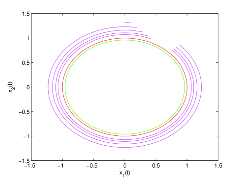
Figure 6: The red orbit of system (4.54) non-axially grazes the surface $\Gamma.$ The magenta trajectory with initial point $(0,1.32)$ approaches the cycle as time increases. The green cycle with initial point $(0,0.96)$ demonstrates the inside stability of the grazing orbit.

5 Small parameter analysis and grazing bifurcation

In this part, we will discuss existence and bifurcation of cycles for perturbed systems, if the generating one admits a grazing periodic solution. In continuous dynamical systems, a small parameter may cause a change in the number of periodic solutions in critical cases. In the present analysis, we will demonstrate that the change may happen in non-critical cases, since of the non-transversality. That is why, one can say that grazing bifurcation is under discussion. Let us deal with the following system

$$x^{\prime}=f(x)+\mu g(x,\mu),$$ (5.61)

$$\Delta x|_{x\in\Gamma(\mu)}=I(x)+\mu K(x,\mu),$$

where $x\in\mathbb{R}^{n},t\in\mathbb{R},\Gamma(\mu)=\{x|\ \Phi(x)+\mu\phi(x,\mu)=0\},$ $\mu\in(-\mu_{0},\mu_{0}),$ and $\mu_{0}$ is a sufficiently small positive number. Functions $f(x),I(x)$ and $\Phi(x)$ are continuously differentiable up to second order, $g(x,\mu),K(x,\mu)$ are continuously differentiable in $x$ and $\mu.$ The function $\phi(x,\mu)$ is continuously differentiable in $x$ up to second order and to first order in $\mu.$ We assume that the generating system for (5.61) is the system (2.1) with all conditions assumed for the system, earlier. The main assumption of this section is that (2.1) admits a $\omega-$periodic solution, $\Psi(t).$ Let $\Psi(0)=(\zeta_{1}^{0},\zeta_{2}^{0},\ldots,\zeta_{n}^{0})$ be the initial value of the solution.

Our aim is to find conditions that verify the existence of periodic solutions of (5.61) with a period $\mathscr{T}$ such that for $\mu=0,$ the periodic solutions of (5.61) are turned down to $\Psi(t).$ It is common for the autonomous systems that the period $\mathscr{T}$ does not coincide with $\omega.$ Thus, in the remaining part of the paper, we will consider the period $\mathscr{T}$ as an unknown variable.

Since $\Psi(0)$ is not an equilibrium, there is a number $j=1,2,\ldots,n,$ such that $f_{j}(\zeta_{1}^{0},\zeta_{1}^{0},\ldots,\zeta_{n}^{0})\neq 0.$ In other words, the vector field is transversal to line $x_{j}=\zeta_{j}^{0}$ near the point. Hence, to try points near to $\Psi(0)$ for the periodicity, it is sufficient to consider those with $j-$th coordinate is equal to $\zeta_{j}^{0},$ [31]. For the discontinuous dynamics, the choice of the fixed coordinate can be made easier if the surface of discontinuity is provided with a constant coordinate. We will demonstrate this in examples. Denote the initial values of the intended periodic solution by $\zeta_{1},\zeta_{2},\ldots,\zeta_{n}.$ Assume that one initial value $\zeta_{j}$ is known, i.e. $\zeta_{j}^{0}.$ Thus, the problem contains $n-$many unknowns, they can be presented as $\zeta_{1},\zeta_{2},\ldots,\zeta_{j-1},\zeta_{j+1},\ldots,\zeta_{n},\mathscr{T}.$ Denote the solution of (5.61) by $x_{s}(t,\zeta_{1},\zeta_{2},\ldots,\zeta_{n},\mu)$ with initial conditions $x_{s}(0,\zeta_{1},\zeta_{2},\ldots,\zeta_{n},\mu)=\zeta_{s}.$ To determine the unknowns, we will consider the Poincar$\acute{e}$ criterion, which can be written as

$$\mathscr{S}_{k}(\mathscr{T},\zeta_{1},\zeta_{2},\ldots,\zeta_{n},\mu)\equiv x_{k}(\mathscr{T},\zeta_{1},\zeta_{2},\ldots,\zeta_{n},\mu)-\zeta_{k}=0,\,k=1,2,\ldots,n,$$ (5.62)

where $\zeta_{j}=\zeta_{j}^{0}.$ The equations (5.62) are satisfied with $\mu=0,\mathscr{T}=\omega,\zeta_{i}=\zeta_{i}^{0},i=1,2,\ldots,n,$ since $\Psi(t)$ is the periodic solution.

The following condition for the determinant is also needed in the remaining part paper.

• $$\begin{vmatrix}\frac{\partial(\mathscr{S}_{1}(\omega,\zeta_{1}^{0},\zeta_{2}^{0},\ldots,\zeta_{j-1}^{0},\zeta_{j+1}^{0},\ldots,\zeta_{n}^{0},0))}{\partial\mathscr{T}}&\ldots&\frac{\partial(\mathscr{S}_{1}(\omega,\zeta_{1}^{0},\zeta_{2}^{0},\ldots,\zeta_{j-1}^{0},\zeta_{j+1}^{0},\ldots,\zeta_{n}^{0},0))}{\partial\zeta_{n}}\\ \frac{\partial(\mathscr{S}_{2}(\omega,\zeta_{1}^{0},\zeta_{2}^{0},\ldots,\zeta_{j-1}^{0},\zeta_{j+1}^{0},\ldots,\zeta_{n}^{0},0))}{\partial\mathscr{T}}&\ldots&\frac{\partial(\mathscr{S}_{2}(\omega,\zeta_{1}^{0},\zeta_{2}^{0},\ldots,\zeta_{j-1}^{0},\zeta_{j+1}^{0},\ldots,\zeta_{n}^{0},0))}{\partial\zeta_{n}}\\ \vdots&\ddots&\vdots\\ \frac{\partial(\mathscr{S}_{n}(\omega,\zeta_{1}^{0},\zeta_{2}^{0},\ldots,\zeta_{j-1}^{0},\zeta_{j+1}^{0},\ldots,\zeta_{n}^{0},0))}{\partial\mathscr{T}}&\ldots&\frac{\partial(\mathscr{S}_{n}(\omega,\zeta_{1}^{0},\zeta_{2}^{0},\ldots,\zeta_{j-1}^{0},\zeta_{j+1}^{0},\ldots,\zeta_{n}^{0},0))}{\partial\zeta_{n}}\end{vmatrix}\neq 0$$ (5.63)

Theorem 5.1

Assume that condition $(A6)$ is valid. Then, (5.61) admits a non-trivial periodic solution, which converges in the $B-$ topology to the non-trivial $\omega$-periodic solution of (5.61) as $\mu$ tends to zero.

We will present the following examples to realize our theoretical results.

Example 5.1

In this example, we will consider the perturbed system in case the generating system has a graziness. To show that, let us take into account the following perturbed system

$$x_{1}^{\prime}=x_{2},$$ (5.64)

$$x_{2}^{\prime}=-0.001x_{2}-x_{1},$$

$$\Delta x_{2}|_{x\in\Gamma_{1}}=-(1+R_{1}x_{2}+\mu x_{2})x_{2},$$

$$\Delta x_{2}|_{x\in\Gamma_{2}}=-(1+R_{2}+\mu(x_{2}-\exp(0.001\pi/2))x_{2}.$$

It is easy to see that the system (5.64) is of the form (5.61). For $\mu=0,$ the generating system became (3.14). For the perturbed system (5.64), we will investigate existence of the periodic solution around the grazing periodic solution of (3.14) with the help of Theorem 5.1.

There are two sorts of possible periodic solutions of (5.64) around the grazing one. One of them has two impulse moments during the period since it crosses both lines of discontinuity, i.e. $x_{1}=0$ and $x_{1}=\exp(0.00025\pi).$ The other sort is the periodic solution which does not intersect the line $x_{1}=\exp(0.00025\pi)$ and intersects the line $x_{1}=0.$ We will show the existence of both type of periodic solutions if $|\mu|$ sufficiently small.

Let us start with the second type, assume that the solution for the perturbed system exists and it starts at the point $(0,x_{02}),x_{02}<1$ and does not intersect the line $x_{1}=\exp(0.00025\pi).$ Denote the initial values of the periodic solution by $\zeta_{1}$ and $\zeta_{2}.$ Since the periodic solution necessarily intersects the line $x_{1}=0,$ one can choose $\zeta_{1}\equiv\zeta_{1}^{0}=0.$ By specifying the formula in (5.62) for the system (5.64), it is easy to obtain the following expressions

$$\mathscr{S}_{1}(\mathscr{T},0,\zeta_{2},\mu)=x_{1}(\mathscr{T},0,\zeta_{2},\mu)=0,$$ (5.65)

$$\mathscr{S}_{2}(\mathscr{T},0,\zeta_{2},\mu)=x_{2}(\mathscr{T},0,\zeta_{2},\mu)-\zeta_{2}=0.$$

Next, taking the derivative of the expressions in (5.65), we can obtain the following

$$\begin{vmatrix}\frac{\partial(\mathscr{S}_{1}(\mathscr{T},0,\zeta_{2},\mu))}{\partial\mathscr{T}}&\frac{\partial(\mathscr{S}_{1}(\mathscr{T},0,\zeta_{2},\mu))}{\partial\zeta_{2}}\\ \frac{\partial(\mathscr{S}_{2}(\mathscr{T},0,\zeta_{2},\mu))}{\partial\mathscr{T}}&\frac{\partial(\mathscr{S}_{2}(\mathscr{T},0,\zeta_{2},\mu))}{\partial\zeta_{2}}\end{vmatrix}=\begin{vmatrix}\frac{\partial x_{1}(\omega,0,\zeta_{2}^{0},0)}{\partial\mathscr{T}}&\frac{\partial x_{1}(\omega,0,\zeta_{2}^{0},0)}{\partial\zeta_{2}}\\ \frac{\partial x_{2}(\omega,0,\zeta_{2}^{0},0)}{\partial\mathscr{T}}&\frac{\partial x_{2}(\omega,0,\zeta_{2}^{0},0)}{\partial\zeta_{2}}-1\end{vmatrix}.$$ (5.66)

The determinant (5.66) is calculated by means of the monodromy matrix of (3.14), with the impulse matrix $D_{1}^{(1)}=O_{2},$ i.e.

$$\begin{bmatrix}1&-0.0317\\ 1.0158&-0.1014\end{bmatrix}.$$ (5.67)

Taking into account the system (5.70) with (5.67) at $\zeta_{2}=\zeta_{2}^{0}$ and $\mathscr{T}=\omega$ for $\mu=0,$ one can derive that

$$\begin{vmatrix}\frac{\partial\mathscr{S}_{1}(\omega,0,\zeta_{2}^{0},0)}{\partial\mathscr{T}}&\frac{\partial\mathscr{S}_{1}(\omega,0,\zeta_{2}^{0},0)}{\partial\zeta_{2}}\\ \frac{\partial\mathscr{S}_{2}(\omega,0,\zeta_{2}^{0},0)}{\partial\mathscr{T}}&\frac{\partial\mathscr{S}_{2}(\omega,0,\zeta_{2}^{0},0)}{\partial\zeta_{2}}-1\end{vmatrix}=-0.0317\exp(0.00025\pi)\neq 0.$$ (5.68)

This verifies condition $(A6).$ Thus, condition $(A6)$ is valid, then by utilizing Theorem (5.1), we can assert that the system (5.61) admits a non-trivial periodic solution, which converges in the $B-$ topology to the non-trivial $\omega$-periodic solution of (2.1) as $\mu$ tends to zero.

Now, let us verify that system (5.64) has a circle which intersects the line $x_{1}=\exp(0.00025\pi)$ in the neighborhood of $(\exp(0.00025\pi),0).$ So, the periodic solution will attain two discontinuity moments in a period. Denote the initial values of the periodic solution by $\zeta_{1}$ and $\zeta_{2}.$ To apply the condition $(A6),$ fix one initial value $\zeta_{1}=\zeta_{1}^{0}=0$ of the intended periodic solution and in the light of the expressions (5.62)

$$\mathscr{S}_{1}(\mathscr{T},0,\zeta_{2},\mu)=x_{1}(\mathscr{T},0,\zeta_{2},\mu)=0,$$ (5.69)

$$\mathscr{S}_{2}(\mathscr{T},0,\zeta_{2},\mu)=x_{2}(\mathscr{T},0,\zeta_{2},\mu)-\zeta_{2}=0.$$

Taking the derivative of the expressions (5.69) with respect to variables $\mathscr{T}$ and $\zeta_{2},$ one can obtain the following

$$\begin{vmatrix}\frac{\partial(\mathscr{S}_{2}(\mathscr{T},0,\zeta_{2},\mu))}{\partial\mathscr{T}}&\frac{\partial(\mathscr{S}_{1}(\mathscr{T},0,\zeta_{2},\mu))}{\partial\zeta_{2}}\\ \frac{\partial(\mathscr{S}_{2}(\mathscr{T},0,\zeta_{2},\mu))}{\partial\mathscr{T}}&\frac{\partial(\mathscr{S}_{2}(\mathscr{T},0,\zeta_{2},\mu))}{\partial\zeta_{2}}\end{vmatrix}=\begin{vmatrix}\frac{\partial x_{1}(\omega,0,\zeta_{2}^{0},0)}{\partial\mathscr{T}}&\frac{\partial x_{1}(\omega,0,\zeta_{2}^{0},0)}{\partial\zeta_{2}}\\ \frac{\partial x_{2}(\omega,0,\zeta_{2}^{0},0)}{\partial\mathscr{T}}&\frac{\partial x_{2}(\omega,0,\zeta_{2}^{0},0)}{\partial\zeta_{2}}-1\end{vmatrix}.$$ (5.70)

To determine the above determinant, the monodromy matrix of (3.13) with the jump matrix $D_{i}^{(2)}$ can be evaluated as

$$\begin{bmatrix}1&0.01\\ 0&0.704\end{bmatrix}.$$ (5.71)

For $\mu=0,$ with the values $\omega$ and $\zeta_{2}^{0}$ the determinant (5.70) can be determined as

$$\begin{vmatrix}\frac{\partial(\mathscr{S}_{1}(\omega,0,\zeta_{2}^{0},0))}{\partial\mathscr{T}}&\frac{\partial(\mathscr{S}_{1}(\omega,0,\zeta_{2}^{0},0))}{\partial\zeta_{2}}\\ \frac{\partial(\mathscr{S}_{2}(\omega,0,\zeta_{2}^{0},0))}{\partial\mathscr{T}}&\frac{\partial(\mathscr{S}_{2}(\omega,0,\zeta_{2}^{0},0))}{\partial\zeta_{2}}\end{vmatrix}=\begin{vmatrix}0&0.01\\ -\exp(0.00025\pi)&-0.296\end{vmatrix}=0.01\exp(0.00025\pi)\neq 0.$$ (5.72)

This verifies condition $(A6).$ So, By Theorem 5.1, we can conclude that the perturbed system (5.64) admits a non-trivial $\mathscr{T}(\mu)-$ periodic solution which converges in the $B-$ topology to the non-trivial $\omega$-periodic solution of (3.14) as $\mu$ tends to zero such that $\mathscr{T}(0)=\omega.$

In Fig. 7, some numerical results are provided to show the solutions of system (5.64) with $\mu=0.05.$

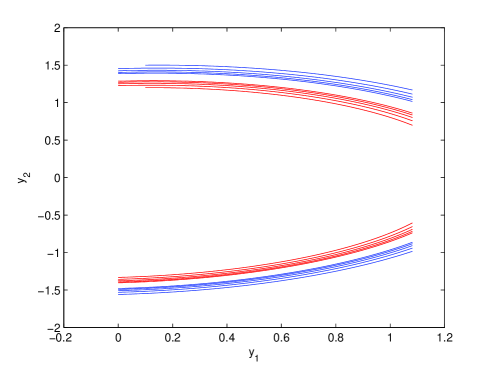
Figure 7: The red arcs are the trajectory of the system (5.64) with initial value $(0,1.2)$ and the blue arcs are the orbit with initial value $(0,1.5).$ Through simulation, we observe that the trajectories approach to the periodic solution of (5.64) as time increases.

The periodic solutions for $\mu\neq 0$ are not grazing. For $\mu=0,$ we have one periodic solution which is orbitally stable, and for $\mu<0,$ there exist two periodic solutions. One of them has one discontinuity moment in each period, in other words, the cycle does not intersect the surface of discontinuity around grazing point and it is orbitally stable and the other one has two discontinuity moments in each period. This means, the number of periodic solutions increases by variation of $\mu,$ around $\mu=0.$ So, we will call that bifurcation of periodic solution from a grazing cycle.

Example 5.2

Let us consider the following system with variable moments of impulses and a small parameter

$$x_{1}^{\prime}=x_{2},$$ (5.73)

$$x_{2}^{\prime}=-0.0001[x_{2}^{2}+(x_{1}-1)^{2}-(1+\mu)^{2}]x_{2}-x_{1}+1,$$

$$\Delta x_{2}|_{x\in\Gamma}=-(1+Rx_{2}+\mu x_{2}^{3})x_{2}+\mu^{2},$$

where $R=0.9$ and $\Gamma=\{x|x_{1}=0,x_{2}\leq 0\}.$ It is easy to see that system (5.73) is of the form (5.61) and $\Phi(x_{1},x_{2})=x_{1}=0.$ The system has a periodic solution

$$\Psi_{\mu}(t)=(1+(1+\mu)\cos(t),-(1+\mu)\sin(t)),$$ (5.74)

where $t\in\mathbb{R}$ for $\mu\in(-2,0].$

The generating system of (5.73) has the following form

$$x_{1}^{\prime}=x_{2},$$ (5.75)

$$x_{2}^{\prime}=-0.0001[x_{2}^{2}+(x_{1}-1)^{2}-1]x_{2}-x_{1}+1,$$

$$\Delta x_{2}|_{x\in\Gamma}=-(1+Rx_{2})x_{2},$$

and admits the periodic solution $\Psi_{0}(t)=(1+\cos(t),-\sin(t)).$ By means of the equality $\langle\nabla\Phi(x^{*}),f(x^{*})\rangle=\langle(1,0),(0,1)\rangle=0$ with $x^{*}=(0,0)\in\partial\Gamma,$ it is easy to say that $x^{*}$ is a grazing point of $\Psi_{0}(t).$

Let us start with the linearization of system (5.75) around the periodic solution $\Psi_{0}(t).$ Consider a near solution $y(t)=y(t,0,y^{*}+\Delta y),$ where $\Delta y=(\Delta y_{1},\Delta y_{2}),$ to the periodic solution $\Psi_{0}(t).$ Assume that $y(t)$ satisfies condition $(N1),$ and it meets the surface of discontinuity $\Gamma$ at the moment $t=\xi$ and at the point $\bar{y}=y(\xi,0,y^{*}+\Delta y).$ Considering the formula (3.10) for the transversal point $\bar{y}=(\bar{y}_{1},\bar{y}_{2}),$ the first component $\displaystyle{\frac{\partial\tau(\bar{y})}{\partial y_{1}^{0}}}$ can be evaluated as $\displaystyle{\frac{\partial\tau(\bar{y})}{\partial y_{1}^{0}}=-\frac{1}{\bar{y}_{2}}}.$ From the last equality, the singularity is seen at the grazing point. By taking into account (3.17) with (5.75) and $\displaystyle{\frac{\partial\tau(\bar{y})}{\partial y_{1}^{0}}},$ we obtain that

$$\displaystyle{\frac{\partial W_{i}(\bar{y})}{\partial y_{1}^{0}}}=\begin{bmatrix}R\bar{y}_{2}-1\\ -0.0001R(\bar{y}_{2}^{2}+(\bar{y}_{1}-1)^{2}-1)-2R(0.0001(\bar{y}_{2}^{2}+(\bar{y}_{1}-1)^{2}-1))\end{bmatrix}.$$ (5.76)

Similarly, taking into account the formula (3.22), one can evaluate that $\displaystyle{\frac{\partial\tau(\bar{y})}{\partial y_{2}^{0}}=0.}$ This and formula (3.1) imply

$$\displaystyle{\frac{\partial W_{i}(\bar{y})}{\partial y_{2}^{0}}}=\begin{bmatrix}0\\ -2R\bar{y}_{2}\end{bmatrix}.$$ (5.77)

Joining (5.76) and (5.77), the matrix $W_{iy}(\bar{y})$ can be obtained as

$$\displaystyle{W_{iy}(\bar{y})}=\begin{bmatrix}R\bar{y}_{2}-1&0\\ -0.0001R(\bar{y}_{2}^{2}+(\bar{y}_{1}-1)^{2}-1)-2R(0.0001(\bar{y}_{2}^{2}+(\bar{y}_{1}-1)^{2}-1))&-2R\bar{y}_{2}\end{bmatrix}.$$ (5.78)

The last expression implies continuity of the partial derivatives near the grazing point. This validates condition $(A2).$

Then, evaluating the matrix in (5.78) at $\bar{y}=y^{*}=(0,0),$ it is easy to obtain

$$\displaystyle{W_{iy}(y^{*})}=\begin{bmatrix}-1&0\\ 0.0003R&0\end{bmatrix},$$ (5.79)

and

$$B_{i}=\begin{cases}O_{2},\quad&\mbox{if }\quad\mbox{ $(N1)$ is valid,}\\ \begin{bmatrix}-1&0\\ 0.0003R&0\end{bmatrix},\quad&\mbox{if }\quad\mbox{ $(N2)$ is valid.}\end{cases}$$ (5.80)

To verify condition $(A3),$ let us specify the region

$$H=\{(y_{1},y_{2})|y_{2}<\sqrt{1-(y_{1}-1)^{2}},\,0\leq y_{1}\leq 1\}.$$

For the grazing solution $\Psi_{0}(t),$ we have that $\theta_{i+1}-\theta_{i}=2\pi.$ Consider a near solution $y(t)=(y_{1}(t),y_{2}(t))=y(t,0,\bar{y})$ to $\Psi(t).$ To satisfy the condition $(N1),$ take $\bar{y}=(\bar{y}_{1},\bar{y}_{2})\in H.$ The orbit of $y(t)$ is below the grazing orbit. Fix points $y=(y_{1},y_{2})\in H$ and $\psi=(\psi_{1},\psi_{2})$ of the orbits $y(t)$ and $\Psi_{0}(t),$ respectively such that $0\leq y_{1}=\psi_{1}\leq 1$ and $\psi_{2}<0.$ Since of the equation $y_{1}^{\prime}=y_{2},$ the speed of $y_{1}(t)$ at $(y_{1},y_{2})$ is larger than the speed of $\Psi_{1}(t)$ at $(\psi_{1},\psi_{2}).$ Consequently, one can find that $\tau(y)\leq\frac{\pi}{4}<2\pi$ for $y\in H.$ Thus, the condition $(A3)$ is valid and Lemma 3.1 verifies the condition $(C).$

It is easy to demonstrate that the condition $(A4)$ is valid such that near solutions to the grazing one are either continuous or discontinuous. That is, they don’t intersect the line of discontinuity $\Gamma$ or intersect it permanently near to the grazing point and by means of the formula (5.80), the linearization system for (5.75) around the grazing cycle $\Psi_{0}(t)$ consists of the following two subsystems

$$u_{1}^{\prime}=u_{2},$$ (5.81)

$$u_{2}^{\prime}=-0.0001\sin(2t)u_{1}+0.0002\sin^{2}(t)u_{2},$$

and

$$u_{1}^{\prime}=u_{2},$$ (5.82)

$$u_{2}^{\prime}=-0.0001\sin(2t)u_{1}+0.0002\sin^{2}(t)u_{2},$$

$$\Delta u|_{2\pi i}=\begin{bmatrix}-1&0\\ 0.0003R&0\end{bmatrix}u.$$

The system (5.81) + (5.82) is $(2\pi,1)$ periodic. The Floquet multipliers of system (5.81) + (5.82) are $\rho_{1}^{(1)}=1,$ $\rho_{2}^{(1)}=0.939,$ $\rho_{1}^{(2)}=1,$ $\rho_{2}^{(2)}=0.912.$ Thus, condition $(A5)$ is validated. Moreover, the conditions $(C1)-(C7)$ and $(A1),(A2)$ can be verified utilizing similar way presented in Example 3.1. Consequently, Theorem 4.1 authenticates that the grazing periodic solution (cycle), $\Psi_{0}(t)$ of the system (5.75) is orbitally stable. The simulation results demonstrating the orbital stability of $\Psi_{0}(t)$ are depicted in Figure 8.

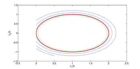
Figure 8: The grazing cycle of system (5.75) is in red. The blue arcs are the trajectory of the system with initial point $(0.5,1.2)$ and the green continuous orbit is with initial value $(0.1,0).$ They demonstrate stability of the grazing solution.

Next, we will investigate two sorts of periodic solutions of system (5.73) with a period $\mathscr{T}$ near to $2\pi.$ The first one is continuous and the second admits discontinuities once on a period. For those solutions, corresponding linearization systems around the grazing cycle $\Psi_{0}(t)$ are (5.81) and (5.82), respectively. Let us start with the continuous periodic solutions of (5.73). For continuous periodic solution, we will consider the linearization system (5.81).

To apply Theorem 5.1, denote $\Psi_{0}(0)=(\zeta_{1}^{0},0).$ That is, consider $\zeta_{2}^{0}=0.$ Then, applying the above discussion, obtain that the Poincar$\grave{e}$ condition admits the form of the following equations,

$$\mathscr{S}_{1}(\mathscr{T},\zeta_{1},\mu)=x_{1}(\mathscr{T},\zeta_{1},\mu)-x_{1}=0,$$ (5.83)

$$\mathscr{S}_{2}(\mathscr{T},\zeta_{1},\mu)=x_{2}(\mathscr{T},\zeta_{1},\mu)=0.$$

Because solutions of the system (5.75) have continuous derivatives with respect to the time, phase variables and parameters, we can calculate the following determinant

$$\begin{vmatrix}\displaystyle{\frac{\partial\mathscr{S}_{1}(\omega,\zeta_{1}^{0},0)}{\partial\mathscr{T}}}&\displaystyle{\frac{\partial\mathscr{S}_{1}(\omega,\zeta_{1}^{0},0)}{\partial x_{1}^{0}}}\\ \displaystyle{\frac{\partial\mathscr{S}_{2}(\omega,\zeta_{1}^{0},0)}{\partial\mathscr{T}}}&\displaystyle{\frac{\partial\mathscr{S}_{2}(\omega,\zeta_{1}^{0},0)}{\partial x_{1}^{0}}}\end{vmatrix}.$$ (5.84)

First, we need the monodromy matrix of the system (5.81). It is

$$\begin{bmatrix}0.939&-0.0001407\\ -0.0003165&1\end{bmatrix}.$$ (5.85)

It is easy to see that first column of the determinant (5.84) is computed by utilizing (5.75) and the second column is evaluated by means of the first column of the matrix (5.85). From this discussion, one can obtain that the determinant (5.84) is equal to

$$\begin{vmatrix}0&-0.061\\ 1&-0.0003165\end{vmatrix}=0.061\neq 0.$$ (5.86)

Thus, in the light of Theorem 5.1, we can conclude that for sufficiently small $|\mu|$ there exists a unique periodic solution of the system

$$x_{1}^{\prime}=x_{2},$$ (5.87)

$$x_{2}^{\prime}=-0.0001[x_{2}^{2}+(x_{1}-1)^{2}-(1+\mu)^{2}]x_{2}-x_{1}+1.$$

It is exactly the cycle (5.74) with a period $\mathscr{T}=2\pi.$ If $\mu<0,$ the solution is separated from the set $\Gamma.$ Consequently, it is a periodic continuous solution of the equation (5.73). It is orbitally stable by the theorem for continuous dynamics [23], since of the continuous dependence of multipliers on the parameter. The function $\Psi_{\mu}(t),\mu>0,$ intersects $\Gamma$ and can not be a solution of equation (5.73). Thus, the system does not admit a continuous periodic solution near to $\Psi_{0}(t),$ if the parameter is positive.

Considering those solutions which have one moment of discontinuity in a period, one can find that the corresponding linearization of $\Psi_{0}(t)$ is the system (5.82).

The monodromy matrix of (5.82) can be evaluated as

$$\begin{bmatrix}0.939&-0.00052\\ -0.000427&1\end{bmatrix}.$$ (5.88)

It can be easily observed that the discontinuous solution intersects the line $x_{1}=0.$ For this reason, one can specify the first coordinate of the initial value as $\zeta_{1}=\zeta_{1}^{0}\equiv 0.$ In the light of these discussions and the formula (5.62), the following equations are obtained:

$$\mathscr{S}_{1}(\mathscr{T},0,\zeta_{2},\mu)=x_{1}(\mathscr{T},0,\zeta_{2},\mu)=0,$$ (5.89)

$$\mathscr{S}_{2}(\mathscr{T},0,\zeta_{2},\mu)=x_{2}(\mathscr{T},0,\zeta_{2},\mu)-\zeta_{2}=0.$$

Then, taking the derivative of the system (5.89) with respect to $\mathscr{T}$ and $\zeta_{2},$ and calculating it at $\mathscr{T}=\omega,$ $\zeta_{2}=\zeta_{2}^{0}=0,$ and for $\mu=0,$ the following determinant is obtained

$$\begin{vmatrix}\displaystyle{\frac{\partial\mathscr{S}_{1}(\omega,0,\zeta_{2}^{0},0)}{\partial\mathscr{T}}}&\displaystyle{\frac{\partial\mathscr{S}_{1}(\omega,0,\zeta_{2}^{0},0)}{\partial\zeta_{2}}}\\ \displaystyle{\frac{\partial\mathscr{S}_{2}(\omega,0,\zeta_{2}^{0},0)}{\partial\mathscr{T}}}&\displaystyle{\frac{\partial\mathscr{S}_{2}(\omega,0,\zeta_{2}^{0},0)}{\partial\zeta_{2}}}\end{vmatrix}=\begin{vmatrix}0&-0.0006\\ 1&0.0009\end{vmatrix}=-0.0006\neq 0.$$ (5.90)

Thus, condition $(A6)$ holds. Then, utilizing Theorem 5.1, it is easy to conclude that for sufficiently small $\mu$ there exists a unique periodic solution of the system (5.73) with a period $\approx 2\pi.$ It is true that for positive as well as negative $\mu.$ Moreover, these solutions are orbitally asymptotically stable because of the continuous dependence of solutions on parameter and initial values and they meet the discontinuity line transversally.

For each fixed $\mu\neq 0,$ solutions near to the periodic ones intersect the line of discontinuity $\Gamma$ transversally once during the time approximately equal to the period. That is, the smoothness which is requested for the application of the Poincar$\grave{e}$ condition is valid, since the smoothness for the grazing point has already been verified. It is clear that there can not be another solutions with period close to $2\pi.$ Thus, one can make the following conclusion. The original system (5.73) admits two orbitally stable periodic solutions, continuous and discontinuous, if $\mu<0.$ There is a single orbitally stable continuous solution (grazing) if $\mu=0.$ Additionally, there is a unique discontinuous orbitally stable periodic solution for positive values of the parameter. Consequently, grazing bifurcation of cycles appears for the system with small parameter.

We have obtained regular behavior in dynamics near grazing orbits by the Poincar$\grave{e}$ small parameter analysis. Nevertheless, outside the attractors irregular phenomena may be observed.

In Figure 9, the solutions of the system (5.73) with parameter $\mu=-0.2$ are depicted through simulations. The red arcs are the trajectory of the system (5.73) with initial value $(0.7,0.05)$ and the blue arcs are the trajectory of the system (5.73) with initial value $(0.4,0.05).$ It is seen that both red and blue trajectories approach the discontinuous periodic solution of (5.73), as time increases. So, the discontinuous cycle is orbitally stable trajectory. Moreover, the green one is a continuous periodic trajectory of (5.73) with initial value $(0,0.05)$ and it is orbitally asymptotically stable. To sum up, there exists two periodic solutions of (5.73) for the parameter $\mu=-0.2,$ one is continuous, the other one is discontinuous and both solutions are orbitally asymptotically stable.

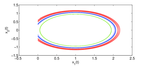
Figure 9: The blue, red and green arcs constitute the trajectories of system (5.73) with $\mu=-0.2.$ The first two approach as time increases to the discontinuous limit cycle and the third one is the continuous limit cycle itself.

In Fig. 10, the red arcs are the orbit of the system with initial value $(0,0.1)$ and the blue arcs are the trajectory of it with initial value $(0,0.4).$ Both trajectories approach to the discontinuous cycle of system (5.73), as time increases. Thus, Fig. 10 illustrates the existence of the orbitally stable discontinuous periodic solution if $\mu=0.2.$

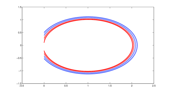
Figure 10: The red and blue arcs constitute the trajectories of the system (5.73) with $\mu=0.2.$ Both orbits approach to the discontinuous limit cycle, as time increases.

6 Conclusion

In literature, the dynamics in the neighborhood of the grazing points [7]-[10], [13], [18], [19], [36]-[39] is generally analyzed through maps of the Poincar$\acute{e}$ type. The main analysis is conducted on complex dynamics behavior such as chaos and bifurcation [7]-[10], [13], [15], [18], [36]-[39]. However, there is still no sufficient conditions for the discontinuous motion to admit main features of dynamical systems : the group property, continuous and differentiable dependence on initial data and continuation of motions, which are useful for both local and global analysis. Variational systems for grazing solutions have not been considered in general as well as orbital stability theorem and regular perturbation theory around cycles, despite, particular cases can be found in specialized papers. See, for example, [12]. To investigate these problems in the present paper, we have applied the method of $B-$ equivalence and results on discontinuous dynamics developed and summarized in [1]. In our analysis the grazing singularity is observed through the gradient of the time function $\tau(x),$ since some of its coordinates are infinite. We have found the components of the discontinuous dynamical system that is the vector field, surfaces of discontinuity and the equations of jump such that interacting they neutralize the effect of singularity. Then, we linearize the system at the grazing moments and this brings the dynamics to regular analysis and make suitable for the application. By means of the linearization, the theory can be understood as a part of the general theory of discontinuous dynamical system. Thus, we have considered grazing phenomena as a subject of the general theory of discontinuous dynamical systems [1], discovered a partition of set of solutions near grazing solution such that we determine linearization around a grazing solution is a collection of several linear impulsive systems with fixed moments of impulses. This constitutes the main novelty of the present paper. To linearize a solution around the grazing one, a system from the collection is to be utilized. This result has been applied to prove the orbital stability theorem. The way of analysis in [1]-[3] continues in the present paper and it admits all attributes which are proper for continuous dynamics [23]. That is why, we believe that the method can be extended for introduction and research of graziness in other types of dynamics such as partial and functional differential equations and others. Next, we plan to apply the present results and the method of investigation for problems initiated in [7]-[10], [37]-[39], [41].

References

- [1] M. Akhmet. Principles of Discontinuous Dynamical Systems. Springer-Verlag, New York, 2010.
- [2] M.U. Akhmet. Perturbations and Hopf bifurcation of the planar discontinuous dynamical system. Nonlinear Analysis, 60:163–178, 2005.
- [3] M.U. Akhmet. On the smoothness of solutions of impulsive autonomous systems, Nonlinear Anal.: TMA, 60:311–324, 2005.
- [4] M. U. Akhmet and A. Kıvılcım. The Models with Impact Deformations, Discontinuity, Nonlinearity, and Complexity, 4(1):49–78, 2015.
- [5] J. Awrejcewicz and CH Lamarque. Bifurcation and Chaos in Nonsmooth Mechanical Systems. World Scientific Series on Nonlinear Science, Singapore, 2003.
- [6] Babitsky V. I., Theory of Vibro-impact systems and applications. Berlin, Heidelberg: Springer-Verlag, 1998.
- [7] M. di Bernardo, Budd C. J., and A.R. Champneys. Grazing bifurcations in n-dimensional piecewise-smooth dynamical systems. Physica D, 160:222–254, 2001.
- [8] M. di Bernardo, Budd C. J., and A.R. Champneys. Grazing, skipping and sliding: analysis of the nonsmooth dynamics of the DC/DC buck converter. Nonlinearity, 11:858–890, 1998.
- [9] M. di Bernardo and S. J. Hogan. Discontinuity-induced bifurcations of piecewise smooth dynamical systems. Philosophical Transactions of The royal society A, 368:4915–4935, 2010.
- [10] M. di Bernardo, C. J. Budd, A.R. Champneys and P. Kowalczyk. Piecewise-smooth dynamical systems theory and applications. Springer-Verlag, London, 2008.
- [11] B. Brogliato. Impacts in Mechanical Systems. Springer-Verlag, Berlin, Heidelberg, 2000.
- [12] B. Brogliato. Nonsmooth mechanics. Springer-Verlag, London, 1999.
- [13] W. Chin, E. Ott, H.E. Nusse, and C. Grebogi. Grazing bifurcations in impact oscillators. Physical Review E, 50:4427–4444, 1994.
- [14] E.A. Coddington, N. Levinson. Theory of Ordinary Differential Equations, McGraw-Hill, New York, 1955.
- [15] V. Donde and I.A. Hiskens. Shooting methods for locating grazing phenomena in hybrid systems. International Journal of Bifurcation and Chaos, 16:3:671–692, 2006.
- [16] E. Falcon, C. Laroche, S. Fauve and C. Coste. Behavior of one inelastic ball bouncing repeatedly off the ground. The European Physical Journal B, 3:45–57, 1998.
- [17] M. Farkas, Periodic Motions, Springer-Verlag, 1994.
- [18] M.I. Feigin. Doubling of the oscillation period with C-bifurcations in piecewise continuous systems. Journal of Applied Mathematics and Mechanics (Prikladnaya Matematika i Mechanika), 34:861–869, 1970.
- [19] M.I. Feigin. On the structure of C-bifurcation boundaries of piecewise continuous systems. Journal of Applied Mathematics and Mechanics (Prikladnaya Matematika i Mechanika), 42:820–829, 1978.
- [20] H. Goldstein. Classical Mechanics. Addison Wesley, United States of America, 1980.
- [21] E. Goursat. A course in mathematical analysis. Gauthier-Villars, 1910.
- [22] P. Hartman. Ordinary Differential Equations. SIAM, 2002.
- [23] M.W. Hirsch, S. Smale and R.L. Devaney Differential Equations, Dynamical Systems, and an Introduction to Chaos, Elsevier, USA, 2004.
- [24] C. Hs and A.R. Champneys. Grazing bifurcations and chatter in a pressure relief valve model. Physica D, 241:2068–2076, 2012.
- [25] R.A. Ibrahim. Vibro-impact Dynamics Modeling, Mapping and Applications. Springer-Verlag, Berlin Heidelberg, 2009.
- [26] A.C.J. Luo. A theory for non-smooth dynamical systems on connectable domains. Communications in Nonlinear Science and Numerical Simulations, 10:1–55, 2005.
- [27] A.C.J. Luo and B. C. Gegg. Grazing phenomena in a periodically forced, friction-induced, linear oscillator. Communications in Nonlinear Science and Numerical Simulations, 11:777–802, 2006.
- [28] A.C.J. Luo. Singularity and Dynamics on Discontinuous Vectorfields, Elsevier, Amsterdam, 2006.
- [29] A.C.J. Luo. Discontinuous Dynamical Systems on Time-varying Domains. Higher Education Press, Beijing, 2009.
- [30] G. Luo, J. Xie , X. Zhu and J. Zhang. Periodic motions and bifurcations of a vibro-impact system. Chaos, Solitons & Fractals, 36:1340–1347, 2008.
- [31] I.G. Malkin. Some Problems in the Theory of Nonlinear Oscillations. State Technical Publishing House, Moscow, 1956.
- [32] D.W. Marhefka and D.E. Orin. A compliant contact model with nonlinear damping for simulation of robotic systems. IEEE Transactions on Systems, Man, and Cybernetics-Part A:Systems and Humans, 29:566–572, 1999.
- [33] S. McNamara and E. Falcon. Simulations of vibrated granular medium with impact velocity dependent restitution coefficient. Physical Review E, 71:031302:1–6, 2005.
- [34] R. K. Miller and A. N. Michel. Ordinary Differential Equations. Academic Press, 1982.
- [35] J. Molenaar, J. G. de Weger and W. van de Water. Mappings of grazing-impact oscillators. Nonlinearity, 14:301–321, 2001.
- [36] A.B. Nordmark. Non-periodic motion caused by grazing incidence in an impact oscillator. Journal of Sound and Vibration, 145:279–297, 1991.
- [37] A.B. Nordmark. Universal limit mapping in grazing bifurcations. Physical Review E, 55:266–270, 1997.
- [38] A.B. Nordmark. Existence of periodic orbits in grazing bifurcations of impacting mechanical oscillators. Nonlinearity, 14:1517–1542, 2001.
- [39] A.B. Nordmark and P.A Kowalczyk. Codimension-two scenario of sliding solutions in grazing-sliding bifurcations.Nonlinearity, 19:1–26, 2006.
- [40] L. Perko. Differential Equations and Dynamical Systems. Springer, 2001.
- [41] P. T. Piiroinen, L. N. Virgin and A. R. Champneys. Chaos and Period-Adding: Experimental and Numerical Verification of the Grazing Bifurcation. J. Nonlinear Sci., 14:383–404, 2004 .
- [42] C. Robinson. Dynamical Systems: Stability, Symbolic Dynamics and Chaos. Studies in Advanced Mathematics, CRC Press, Boca Raton, FL, 1995.
- [43] W. Rudin. Principles of mathematical analysis. McGraw-Hill, 1953.
- [44] P.S. Simeonov and D.D. Bainov. Orbital stability of the periodic solutions of autonomous systems with impulse effect, Publ. RIMS, Kyoto Univ., 25:312–346, 1989.
- [45] A.M. Samoilenko and N.A. Perestyuk. Impulsive Differential Equations. World Scientific Series on Nonlinear Science Series A: Volume 14, 1995.