A generalized nonlinear model for long memory conditional heteroscedasticity

Abstract

We study the existence and properties of stationary solution of ARCH-type equation $r_{t}=\zeta_{t}\sigma_{t}$, where $\zeta_{t}$ are standardized i.i.d. r.v.’s and the conditional variance satisfies an AR(1) equation $\sigma^{2}_{t}=Q^{2}\big{(}a+\sum_{j=1}^{\infty}b_{j}r_{t-j}\big{)}+\gamma\sigma^{2}_{t-1}$ with a Lipschitz function $Q(x)$ and real parameters $a,\gamma,b_{j}$. The paper extends the model and the results in [5] from the case $\gamma=0$ to the case $0<\gamma<1$. We also obtain a new condition for the existence of higher moments of $r_{t}$ which does not include the Rosenthal constant. In the particular case when $Q$ is the square root of a quadratic polynomial, we prove that $r_{t}$ can exhibit a leverage effect and long memory. We also present simulated trajectories and histograms of marginal density of $\sigma_{t}$ for different values of $\gamma$.

Keywords: asymmetric ARCH model, LARCH model, leverage, long memory

1 Introduction

Doukhan et al. [5] discussed the existence of stationary solution of conditionally heteroscedastic equation

$$r_{t} = \zeta_{t}\sigma_{t},\qquad\sigma^{2}_{t}\ =\ Q^{2}\Big{(}a+\sum_{j=1}^{\infty}b_{j}r_{t-j}\Big{)},$$ (1.1)

where $\{\zeta_{t}\}$ are standardized i.i.d. r.v.’s, $a,b_{j}$ are real parameters and $Q(x)$ is a Lipschitz function of real variable $x\in\mathbb{R}$. Probably, the most important case of (1.1) is

$$Q(x)=\sqrt{c^{2}+x^{2}},$$ (1.2)

where $c\geq 0$ is a parameter. The model (1.1)-(1.2) includes the classical Asymmetric ARCH(1) of Engle [7] and the Linear ARCH (LARCH) model of Robinson [16]:

$$r_{t}\ =\ \zeta_{t}\sigma_{t},\qquad\sigma_{t}\ =\ a+\beta\sum_{j=1}^{\infty}j^{d-1}r_{t-j}.$$ (1.3)

[9] proved that the squared stationary solution $\{r^{2}_{t}\}$ of the LARCH model in (1.3) with $b_{j}$ decaying as $j^{d-1},0<d<1/2$ may have long memory autocorrelations. The leverage effect in the LARCH model was discussed in detail in [10]. Doukhan et al. [5] extended the above properties of the LARCH model (long memory and leverage) to the model in (1.1)-(1.2) with $c>0$ or strictly positive volatility.

The present paper extends the results of [5] to a more general class of volatility forms:

$$r_{t} = \zeta_{t}\sigma_{t},\qquad\sigma^{2}_{t}\ =\ Q^{2}\Big{(}a+\sum_{j=1}^{\infty}b_{j}r_{t-j}\Big{)}+\gamma\sigma^{2}_{t-1},$$ (1.4)

where $\{\zeta_{t}\},a,b_{j},Q(x)$ are as in (1.1) and $0<\gamma<1$ is a parameter. The inclusion of lagged $\sigma^{2}_{t-1}$ in (1.4) helps to reduce very sharp peaks and clustering of volatility which occur in trajectory of (1.1)-(1.2) near the threshhold $c>0$ (see Fig. 1). The generalization from (1.1) to (1.4) is similar to that from ARCH to GARCH models, see [6], [3], particularly, (1.4) with $Q(x)$ of $\eqref{Qform1}$ and $b_{j}=0,j\geq 2$ reduces to the Asymmetric GARCH(1,1) of Engle [7].

Let us describe the main results of this paper. Sec. 2 (Theorems 4 and 5) obtain sufficient conditions for the existence of stationary solution of (1.4) with $\mathrm{E}|r_{t}|^{p}<\infty$ and $\gamma\in[0,1)$. Theorem 4 extends the corresponding result in ([5], Thm. 4) from $\gamma=0$ to $\gamma>0$. Theorem 5 is new even in the case $\gamma=0$ by providing an explicit sufficient condition (2.25) for higher-order even moments ($p=4,6,\dots$) which does not involve the absolute constant in the Burkholder-Rosenthal inequality (2.11). Condition (2.25) coincides with the corresponding moment condition for the LARCH model and is important for statistical applications, see Remark 2. The remaining sec. 3-5 deal exclusively with the case of quadratic $Q^{2}$ in (1.2), referred to as the Generalized Quadratic ARCH (GQARCH) model in the sequel. Theorem 6 (sec. 3) obtains long memory properties of the squared process $\{r^{2}_{t}\}$ of the GQARCH model with $\gamma\in(0,1)$ and coefficients $b_{j}$ decaying regularly as $b_{j}\sim\beta j^{d-1},\,j\to\infty,\,0<d<1/2$. Similar properties were established in [5] for the GQARCH model with $\gamma=0$ and for the LARCH model (1.3) in [9], [10]. Quasi-maximum likelihood estimation for parametric GQARCH model with long memory was recently studied in [13]. See the review paper [11] and recent work [12] on long memory ARCH modeling. Sec. 4 extends to the GQARCH model the leverage effect discussed in [5] and [10]. Sec. 5 presents some simulations and volatility profiles for the LARCH and GQARCH models with parameters estimated from real data. A general impression from our results is that the GQARCH modification in (1.4), (1.2) of the QARCH model in [5] allows for a more realistic volatility modeling as compared to the LARCH and QARCH models, at the same time preserving the long memory and the leverage properties of the above mentioned models.

2 Stationary solution

Denote $|\mu|_{p}:=\mathrm{E}|\zeta_{0}|^{p}\,(p>0),\,\mu_{p}:=\mathrm{E}\zeta_{0}^{p}\,(p=1,2,\dots)$ and let

$$X_{t}\ :=\ \sum_{s<t}b_{t-s}r_{s}.$$ (2.5)

Since $0\leq\gamma<1$, equations (1.4) yield

$$\sigma^{2}_{t} = \sum_{\ell=0}^{\infty}\gamma^{\ell}Q^{2}(a+X_{t-\ell})\quad\text{and}\quad r_{t}\ =\ \zeta_{t}\sqrt{\sum_{\ell=0}^{\infty}\gamma^{\ell}Q^{2}(a+X_{t-\ell})}.$$ (2.6)

In other words, stationary solution of (1.4), or

$$r_{t}\ =\ \zeta_{t}\sqrt{\sum_{\ell=0}^{\infty}\gamma^{\ell}Q^{2}(a+\sum_{j=1}^{\infty}b_{j}r_{t-\ell-j})}$$ (2.7)

can be defined via (2.5), or stationary solution of

$$X_{t}\ :=\ \sum_{s<t}b_{t-s}\zeta_{s}\sqrt{\sum_{\ell=0}^{\infty}\gamma^{\ell}Q^{2}(a+X_{s-\ell})},$$ (2.8)

and vice versa.

In Theorem 4 below, we assume that $Q$ in (2.6) is a Lipschitz function, i.e., there exists ${\rm Lip}_{Q}>0$ such that

$$|Q(x)-Q(y)|\leq{\rm Lip}_{Q}|x-y|,\qquad x,y\in\mathbb{R}.$$ (2.9)

Note (2.9) implies the bound

$$Q^{2}(x)\leq c_{1}^{2}+c_{2}^{2}x^{2},\qquad x\in\mathbb{R},$$ (2.10)

where $c_{1}\geq 0,\,c_{2}\geq{\rm Lip}_{Q}$ and $c_{2}$ can be chosen arbitrarily close to ${\rm Lip}_{Q}$.

Let us give some formal definitions. Let ${\cal F}_{t}=\sigma(\zeta_{s},s\leq t),t\in\mathbb{Z}$ be the sigma-field generated by $\zeta_{s},s\leq t$. A random process $\{u_{t},t\in\mathbb{Z}\}$ is called adapted (respectively, predictable) if $u_{t}$ is ${\cal F}_{t}$-measurable for each $t\in\mathbb{Z}$ (respectively, $u_{t}$ is ${\cal F}_{t-1}$-measurable for each $t\in\mathbb{Z}$).

Definition 1

Let $p>0$ be arbitrary.

(i) By $L^{p}$-solution of (2.6) or/and (2.7) we mean an adapted process $\{r_{t},t\in\mathbb{Z}\}$ with $\mathrm{E}|r_{t}|^{p}<\infty$ such that for any $t\in\mathbb{Z}$ the series $X_{t}=\sum_{j=1}^{\infty}b_{j}r_{t-j}$ converges in $L^{p}$, the series $\sigma^{2}_{t}=\sum_{\ell=0}^{\infty}\gamma^{\ell}Q^{2}(a+X_{t-\ell})$ converges in $L^{p/2}$ and (2.7) holds.

(ii) By $L^{p}$-solution of (2.8) we mean a predictable process $\{X_{t},t\in\mathbb{Z}\}$ with $\mathrm{E}|X_{t}|^{p}<\infty$ such that for any $t\in\mathbb{Z}$ the series $\sigma^{2}_{t}=\sum_{\ell=0}^{\infty}\gamma^{\ell}Q^{2}(a+X_{t-\ell})$ converges in $L^{p/2}$, the series $\sum_{s<t}b_{t-s}\zeta_{s}\sigma_{s}$ converges in $L^{p}$ and (2.8) holds.

Define

$$B_{p}:=\begin{cases}\sum_{j=1}^{\infty}|b_{j}|^{p},&0<p<2,\\ \big{(}\sum_{j=1}^{\infty}b_{j}^{2}\big{)}^{p/2},&p\geq 2,\end{cases}\qquad B_{p,\gamma}:=\begin{cases}B_{p}/(1-\gamma^{p/2}),&0<p<2,\\ B_{p}/(1-\gamma)^{p/2},&p\geq 2.\end{cases}$$

Note $B_{p}=B_{p,0}$. As in [5], we use the following moment inequality, see [4], [20], [17].

Proposition 2

Let $\{Y_{j},j\geq 1\}$ be a sequence of r.v.’s such that $\mathrm{E}|Y_{j}|^{p}<\infty$ for some $p>0$. If $p>1$ we additionally assume that $\{Y_{j}\}$ is a martingale difference sequence: $\mathrm{E}[Y_{j}|Y_{1},\dots,Y_{j-1}]=0,\,j=2,3,\dots$. Then there exists a constant $K_{p}\geq 1$ depending only on $p$ and such that

$$\mathrm{E}\big{|}\sum_{j=1}^{\infty}Y_{j}\big{|}^{p}\ \leq\ K_{p}\begin{cases}\sum_{j=1}^{\infty}\mathrm{E}|Y_{j}|^{p},&0<p\leq 2,\\ \big{(}\sum_{j=1}^{\infty}(\mathrm{E}|Y_{j}|^{p})^{2/p}\big{)}^{p/2},&p>2.\end{cases}$$ (2.11)

Proposition 3 says that equations (2.7) and (2.8) are equivalent in the sense that by solving one the these equations one readily obtains a solution to the other one.

Proposition 3

Let $Q$ be a measurable function satisfying (2.10) with some $c_{1},c_{2}\geq 0$ and $\{\zeta_{t}\}$ be an i.i.d. sequence with $|\mu|_{p}=\mathrm{E}|\zeta_{0}|^{p}<\infty$ and satisfying $\mathrm{E}\zeta_{0}=0$ for $p>1$. In addition, assume $B_{p}<\infty$ and $0\leq\gamma<1$.

(i) Let $\{X_{t}\}$ be a stationary $L^{p}$-solution of (2.8) and let $\sigma_{t}:=\sqrt{\sum_{\ell=0}^{\infty}\gamma^{\ell}Q^{2}(a+X_{t-\ell})}$. Then $\{r_{t}=\zeta_{t}\sigma_{t}\}$ in (2.6) is a stationary $L^{p}$-solution of (2.7) and

$$\mathrm{E}|r_{t}|^{p}\ \leq\ C(1+\mathrm{E}|X_{t}|^{p}).$$ (2.12)

Moreover, for $p>1$, $\{r_{t},{\cal F}_{t},t\in\mathbb{Z}\}$ is a martingale difference sequence with

$$\mathrm{E}[r_{t}|{\cal F}_{t-1}]=0,\qquad\mathrm{E}[|r_{t}|^{p}|{\cal F}_{t-1}]=|\mu|_{p}\sigma_{t}^{p}.$$ (2.13)

(ii) Let $\{r_{t}\}$ be a stationary $L^{p}$-solution of (2.7). Then $\{X_{t}\}$ in (2.5) is a stationary $L^{p}$-solution of (2.8) such that

$$\mathrm{E}|X_{t}|^{p}\ \leq\ C\mathrm{E}|r_{t}|^{p}.$$

Moreover, for $p\geq 2$

$$\mathrm{E}[X_{t}X_{0}]\ =\ \mathrm{E}r^{2}_{0}\sum_{s=1}^{\infty}b_{t+s}b_{s},\qquad t=0,1,\dots.$$

Proof. (i) First, let $0<p\leq 2$. Then $\mathrm{E}|\sigma_{t}|^{p}=\mathrm{E}|\sigma^{2}_{t}|^{p/2}\leq\sum_{\ell=0}^{\infty}|\gamma^{p/2}|^{\ell}\mathrm{E}|Q(a+X_{t-\ell})|^{p}<\infty.$ Hence, using (2.10), the fact that $\{X_{t}\}$ is predictable and $|Q(a+X_{t-\ell})|^{p}\leq|c_{1}^{2}+c_{2}^{2}(a+X_{t-\ell})|^{p/2}\leq C(1+|a+X_{t-\ell}|^{p})\leq C(1+|X_{t-\ell}|^{p})$ we obtain

$$\mathrm{E}|r_{t}|^{p} = |\mu|_{p}\mathrm{E}|\sigma_{t}|^{p}\ \leq\ C\sum_{\ell=0}^{\infty}|\gamma^{p/2}|^{\ell}(1+\mathrm{E}|X_{t-\ell}|^{p})$$

$$\leq C(1+\mathrm{E}|X_{t}|^{p})\ <\ \infty,$$

proving (2.12) for $p\leq 2$. Next, let $p>2$. Then $\mathrm{E}|\sigma_{t}|^{p}\leq(\sum_{\ell=0}^{\infty}\gamma^{\ell}\mathrm{E}^{2/p}|Q(a+X_{t})|^{p})^{p/2}\leq C\mathrm{E}|Q(a+X_{t})|^{p}$ by stationarity and Minkowski’s inequality and hence (2.12) follows using the same argument as above. Clearly, for $p>1$ $\{r_{t}=\zeta_{t}\sigma_{t}\}$ is a martingale difference sequence and satisfies (2.13). Then, the convergence in $L^{p}$ of the series in (2.5) follows from (2.12) and Proposition 2:

$$\mathrm{E}|\sum_{j=1}^{\infty}b_{j}r_{t-j}|^{p} \leq C\left\{\begin{array}[]{ll}\sum_{j=1}^{\infty}|b_{j}|^{p},&0<p\leq 2\\ \big{(}\sum_{j=1}^{\infty}b_{j}^{2}\big{)}^{p/2},&p>2\end{array}\right\}\ =\ CB_{p}\ <\ \infty.$$

In particular, $\zeta_{t}\sqrt{\sum_{\ell=0}^{\infty}\gamma^{\ell}Q^{2}(a+\sum_{s<t}b_{t-\ell-s}r_{s})}=\zeta_{t}\sqrt{\sum_{\ell=0}^{\infty}\gamma^{\ell}Q^{2}(a+X_{t-\ell})}=r_{t}$ by the definition of $r_{t}$. Hence, $\{r_{t}\}$ is a $L^{p}$-solution of (2.7). Stationarity of $\{r_{t}\}$ follows from stationarity of $\{X_{t}\}$.

(ii) Since $\{r_{t}\}$ is a $L^{p}$-solution of (2.7), so $r_{t}=\zeta_{t}\sigma_{t}=\zeta_{t}\sqrt{\sum_{\ell=0}^{\infty}\gamma^{\ell}Q^{2}(a+X_{t-\ell})}$ with $X_{t}$ defined in (2.5) and $\{X_{t}\}$ satisfy (2.5), where the series converges in $L^{p}$. The rest follows as in [5], proof of Prop.3. $\Box$

Remark 1

Let $p\geq 2$ and $|\mu|_{p}<\infty$, then by inequality (2.11), $\{r_{t}\}$ being a stationary $L^{p}$-solution of (2.6) is equivalent to $\{r_{t}\}$ being a stationary $L^{2}$-solution of (2.6) with $\mathrm{E}|r_{0}|^{p}<\infty$. Similarly, if $Q$ and $\{\zeta_{t}\}$ satisfy the conditions of Proposition 3 and $p\geq 2$, then $\{X_{t}\}$ being a stationary $L^{p}$-solution of (2.5) is equivalent to $\{X_{t}\}$ being a stationary $L^{2}$-solution of (2.5) with $\mathrm{E}|X_{0}|^{p}<\infty$. See also ([5], Remark 1).

Theorem 4

Let $\{\zeta_{t}\}$ satisfy the conditions of Proposition 3 and $Q$ satisfy the Lipschitz condition in (2.9).

(i) Let $p>0$ and

$$K^{1/p}_{p}\,|\mu|^{1/p}_{p}\,{\rm Lip}_{Q}\,B^{1/p}_{p,\gamma}<1,$$ (2.15)

where $K_{p}$ is the absolute constant from the moment inequality in (2.11). Then there exists a unique stationary $L^{p}$-solution $\{X_{t}\}$ of (2.8) and

$$\mathrm{E}|X_{t}|^{p}\ \leq\frac{C(p,Q)|\mu|_{p}B_{p}}{1-K_{p}|\mu|_{p}{\rm Lip}_{Q}^{p}B_{p,\gamma}},$$ (2.16)

where $C(p,Q)<\infty$ depends only on $p$ and $c_{1},c_{2}$ in (2.10).

(ii) Assume, in addition, that $Q^{2}(x)=c_{1}^{2}+c_{2}^{2}x^{2}$, where $c_{i}\geq 0,i=1,2$, and $\mu_{2}=\mathrm{E}\zeta^{2}_{0}=1$. Then $c^{2}_{2}B_{2,\gamma}<1$ is a necessary and sufficient condition for the existence of a stationary $L^{2}$-solution $\{X_{t}\}$ of (2.8) with $a\neq 0$.

Proof. (i) We follow the proof of Theorem 4 in [5]. For $n\in\mathbb{N}$ we recurrently define a solution of (2.8) with zero initial condition at $t\leq-n$ as

$$X^{(n)}_{t} := \begin{cases}0,&t\leq-n,\\ \sum_{s=-n}^{t-1}b_{t-s}\zeta_{s}\sigma^{(n)}_{s},&t>-n,\quad t\in\mathbb{Z},\end{cases}$$ (2.17)

where $\sigma^{(n)}_{s}:=\sqrt{\sum_{\ell=0}^{n+s}\gamma^{\ell}Q^{2}(a+X^{(n)}_{s-\ell})}$. Let us show that $\{X^{(n)}_{t}\}$ converges in $L^{p}$ to a stationary $L^{p}$-solution $\{X_{t}\}$ as $n\to\infty$.

First, let $0<p\leq 2$. Let $m>n\geq 0$. Then by inequality (2.11) for any $t>-m$ we have that

$$\mathrm{E}|X^{(m)}_{t}-X^{(n)}_{t}|^{p} \leq K_{p}|\mu|_{p}\Big{\{}\sum_{-m\leq s<-n}|b_{t-s}|^{p}\mathrm{E}|\sigma^{(m)}_{s}|^{p}+\sum_{-n\leq s<t}|b_{t-s}|^{p}\mathrm{E}|\sigma^{(m)}_{s}-\sigma^{(n)}_{s}|^{p}\Big{\}}$$ (2.18)

$$=:K_{p}|\mu|_{p}\big{\{}S^{\prime}_{m,n}+S^{\prime\prime}_{m,n}\big{\}}.$$

Using $|Q(a+x)|^{p}\leq C+c_{3}^{p}|x|^{p},x\in\mathbb{R}$ with $c_{3}>c_{2}>{\rm Lip}_{Q}$ arbitrarily close to ${\rm Lip}_{Q}$, see [5], proof of Theorem 4, we obtain

$$S^{\prime}_{m,n} \leq \sum_{-m\leq s<-n}|b_{t-s}|^{p}\sum_{\ell=0}^{m+s}\gamma^{p\ell/2}(C+c_{3}^{p}\mathrm{E}|X^{(m)}_{s-\ell}|^{p}).$$ (2.19)

Next, using $|(\sum_{i>0}\gamma^{i}x_{i}^{2})^{1/2}-(\sum_{i>0}\gamma^{i}y_{i}^{2})^{1/2}|\leq(\sum_{i>0}\gamma^{i}(x_{i}-y_{i})^{2})^{1/2}$ we obtain

$$|\sigma^{(m)}_{s}-\sigma^{(n)}_{s}|\leq\left(\sum_{\ell=0}^{s+n}\gamma^{\ell}\big{(}Q(a+X^{(m)}_{s-\ell})-Q(a+X^{(n)}_{s-\ell})\big{)}^{2}+\sum_{\ell=s+n+1}^{s+m}\gamma^{\ell}Q^{2}(a+X^{(m)}_{s-\ell})\right)^{1/2}.$$ (2.20)

Hence from the Lipschitz condition in (2.9) we have that

$$S^{\prime\prime}_{m,n} \leq \sum_{-n\leq s<t}|b_{t-s}|^{p}\left(\sum_{\ell=0}^{s+n}\gamma^{p\ell/2}{\rm Lip}_{Q}^{p}\mathrm{E}|X^{(m)}_{s-\ell}-X^{(n)}_{s-\ell}|^{p}+\sum_{\ell=s+n+1}^{s+m}\gamma^{p\ell/2}(C+c_{3}^{p}\mathrm{E}|X^{(m)}_{s-\ell})|^{p})\right).$$

Combining (2.18) and the above bounds we obtain

$$\mathrm{E}|X^{(m)}_{t}-X^{(n)}_{t}|^{p} \leq K_{p}|\mu|_{p}\Big{(}c_{3}^{p}\sum_{-m\leq s<t}|b_{t-s}|^{p}\sum_{\ell=0}^{s+m}\gamma^{p\ell/2}\mathrm{E}|X^{(m)}_{s-\ell}-X^{(n)}_{s-\ell}|^{p}$$ (2.21)

$$+ \quad C\sum_{-m\leq s<-n}|b_{t-s}|^{p}\sum_{\ell=0}^{s+m}\gamma^{p\ell/2}+C\sum_{-n\leq s<t}|b_{t-s}|^{p}\sum_{\ell=s+n+1}^{s+m}\gamma^{p\ell/2}\Big{)}$$

$$\leq CK_{p}|\mu|_{p}\kappa^{p}_{t+n,\gamma}+K_{p}|\mu|_{p}c_{3}^{p}\sum_{-m\leq s<t}b_{t-s,\gamma}^{p}\mathrm{E}|X^{(n)}_{s}-X^{(m)}_{s}|^{p}.$$

where $b_{s,\gamma}^{p}:=\sum_{j=0}^{s-1}\gamma^{jp/2}|b_{s-j}|^{p},s\geq 0,\kappa_{t+n}:=C(1-\gamma^{p/2})^{-1}K_{p}|\mu|_{p}(\sum_{j>t+n}|b_{j}|^{p}+b_{t+n,\gamma}^{p})\to 0\,(n\to\infty)$.

Iterating inequality (2.21) as in [5], (6.55) and using $K_{p}|\mu|_{p}c_{3}^{p}\sum_{s<t}b_{t-s,\gamma}^{p}=K_{p}|\mu|_{p}c_{3}^{p}B_{p,\gamma}<1$ we obtain $\lim_{m,n\to\infty}\mathrm{E}|X^{(m)}_{t}-X^{(n)}_{t}|^{p}=0$ and hence the existence of $X_{t}$ such that $\lim_{n\to\infty}\mathrm{E}|X^{(n)}_{t}-X_{t}|^{p}=0$ and satisfying the bound in (2.16).

Next, consider the case $p>2$. Let $m>n\geq 0$. Then by inequality (2.11) for any $t>-m$ we have that

$$\mathrm{E}|X^{(m)}_{t}-X^{(n)}_{t}|^{p} \leq K_{p}|\mu|_{p}\Big{(}\sum_{-m\leq s<-n}b^{2}_{t-s}\mathrm{E}^{2/p}|\sigma^{(m)}_{s}|^{p}+\sum_{-n\leq s<t}b^{2}_{t-s}\mathrm{E}^{2/p}|\sigma^{(m)}_{s}-\sigma^{(n)}_{s}|^{p}\Big{)}^{p/2}$$ (2.22)

$$=:K_{p}|\mu|_{p}\big{(}R^{\prime}_{m,n}+R^{\prime\prime}_{m,n}\big{)}^{p/2}.$$

Similarly to (2.19),

$$R^{\prime}_{m,n} \leq \sum_{s=-m}^{-n-1}b^{2}_{t-s}\sum_{\ell=0}^{m+s}\gamma^{\ell}\mathrm{E}^{2/p}|Q(a+X^{(m)}_{s-\ell})|^{p}\ \leq\ \sum_{s=-m}^{-n-1}b^{2}_{t-s}\sum_{\ell=0}^{m+s}\gamma^{\ell}(C+c^{2}_{3}\mathrm{E}^{2/p}|X^{(m)}_{s-\ell}|^{p})$$

and, using (2.20),

$$R^{\prime\prime}_{m,n} \leq \sum_{-n\leq s<t}b^{2}_{t-s}\mathrm{E}^{2/p}\Big{|}\sum_{\ell=0}^{s+n}\gamma^{\ell}(Q(a+X^{(m)}_{s-\ell})-Q(a+X^{(n)}_{s-\ell}))^{2}+\sum_{\ell=s+n+1}^{s+m}\gamma^{\ell}Q^{2}(a+X^{(m)}_{s-\ell})\Big{|}^{p/2}$$

$$\leq \sum_{-n\leq s<t}b^{2}_{t-s}\Big{(}\sum_{\ell=0}^{s+n}\gamma^{\ell}\mathrm{E}^{2/p}|Q(a+X^{(m)}_{s-\ell})-Q(a+X^{(n)}_{s-\ell})|^{p}+\sum_{\ell=s+n+1}^{s+m}\gamma^{\ell}\mathrm{E}^{2/p}|Q(a+X^{(m)}_{s-\ell})|^{p}\Big{)}$$

$$\leq \sum_{-n\leq s<t}b^{2}_{t-s}\Big{(}{\rm Lip}^{2}_{Q}\sum_{\ell=0}^{s+n}\gamma^{\ell}\mathrm{E}^{2/p}|X^{(m)}_{s-\ell}-X^{(n)}_{s-\ell}|^{p}+\sum_{\ell=s+n+1}^{s+m}\gamma^{\ell}(C+c_{3}^{2}\mathrm{E}^{2/p}|X^{(m)}_{s-\ell}|^{p})\Big{)}$$

Consequently,

$$\mathrm{E}^{2/p}|X^{(m)}_{t}-X^{(n)}_{t}|^{p} \leq \kappa_{t+n}+K^{2/p}_{p}|\mu|_{p}^{2/p}c^{2}_{3}\sum_{-m\leq s<t}b^{2}_{t-s,\gamma}\mathrm{E}^{2/p}|X^{(m)}_{s})-X^{(n)}_{s}|^{p},$$

where $\kappa_{t+n}:=C(1-\gamma)^{-1}K^{2/p}_{p}|\mu|_{p}^{2/p}(\sum_{j>t+n}b^{2}_{j}+b_{t+n,\gamma}^{2})\to 0\,(n\to\infty)$. By iterating the last displayed equation and using $K^{2/p}_{p}|\mu|_{p}^{2/p}c^{2}_{3}\sum_{j=1}b^{2}_{j,\gamma}=K^{2/p}_{p}|\mu|_{p}^{2/p}c^{2}_{3}B_{2}/(1-\gamma)<1$ we obtain $\lim_{m,n\to\infty}\mathrm{E}^{2/p}|X^{(m)}_{t}-X^{(n)}_{t}|^{p}=0$ and hence the existence of $X_{t}$ such that $\lim_{n\to\infty}\mathrm{E}|X^{(n)}_{t}-X_{t}|^{p}=0$ and satisfying the bound in (2.16). The rest of the proof of part (i) is similar as in [5], proof of Theorem 4, and we omit the details.

(ii) Note that $Q(x)=\sqrt{c_{1}^{2}+c_{2}^{2}x^{2}}$ is a Lipschitz function and satisfies (2.9) with ${\rm Lip}_{Q}=c_{2}$. Hence by $K_{2}=1$ and part (i), a unique $L^{2}$-solution $\{X_{t}\}$ of (2.8) under the condition $c^{2}_{2}B_{2,\gamma}=c_{2}^{2}B_{2}/(1-\gamma)<1$ exists. To show the necessity of the last condition, let $\{X_{t}\}$ be a stationary $L^{2}$-solution of (2.8). Then

$$\mathrm{E}X^{2}_{t} = \sum_{s<t}b^{2}_{t-s}\sum_{\ell=0}^{\infty}\gamma^{\ell}\mathrm{E}Q^{2}(a+X_{s-\ell})$$

$$= \sum_{s<t}b^{2}_{t-s}\sum_{\ell=0}^{\infty}\gamma^{\ell}\mathrm{E}\big{(}c_{1}^{2}+c_{2}^{2}(a+X_{s-\ell}^{2}\big{)}$$

$$= (B_{2}/(1-\gamma))\big{(}c_{1}^{2}+c^{2}_{2}(a^{2}+\mathrm{E}X^{2}_{t})\big{)}\ >c^{2}_{2}(B_{2}/(1-\gamma))\mathrm{E}X^{2}_{t}$$

since $a\neq 0$. Hence, $c^{2}_{2}B_{2}/(1-\gamma)<1$ unless $\mathrm{E}X^{2}_{t}=0$, or $\{X_{t}=0\}$ is a trivial process. Clearly, (2.8) admits a trivial solution if and only if $0=Q(a)=\sqrt{c_{1}^{2}+c_{2}^{2}a^{2}}=0,$ or $c_{1}=c_{2}=0$. This proves part (ii) and the theorem. $\Box$

Remark 2

Theorem 4 extends ([5], Thm. 4) from $\gamma=0$ to $\gamma>0$. A major shortcoming of Theorem 4 and the above mentioned result in [5] is the presence of the universal constant $K_{p}$ whose upper bound given in [15] leads to restrictive conditions on $B_{p,\gamma}$ in (2.15) for the existence of $L^{p}$-solution, $p>2$. For example, for $p=4$ the above mentioned bound in [15] gives

$$K_{4}\mu_{4}B_{2}^{2}/(1-\gamma)^{2}\leq(27.083)^{4}\mu_{4}B_{2}^{2}/(1-\gamma)^{2}<1$$ (2.23)

requiring $B_{2}=\sum_{j=1}^{\infty}b^{2}_{j}$ to be very small. Since statistical inference based of ‘observable’ squares $r^{2}_{t},1\leq t\leq n$ usually requires the existence of $\mathrm{E}r^{4}_{t}$ and higher moments of $r_{t}$ (see e.g. [13]), the question arises to derive less restrictive conditions for the existence of these moments which do not involve the Rosenthal constant $K_{p}$. This is achieved in the subsequent Theorem 5. Particularly, for $\gamma=0,{\rm Lip}_{Q}=1$ the sufficient condition (2.25) of Theorem 5 for the existence of $\mathrm{E}r^{p}_{t},p\geq 2$ even becomes

$$\sum_{j=2}^{p}{p\choose j}|\mu_{j}|\sum_{k=1}^{\infty}|b_{k}|^{j}\ <\ 1.$$ (2.24)

Condition (2.24) coincides with the corresponding condition in the LARCH case in ([10], Proposition 3). Moreover, (2.24) and (2.25) apply to more general classes of ARCH models in (1.1) and (1.4) to which the specific Volterra series techniques used in [9], [10] are not applicable. In the particular case $p=4$ condition (2.24) becomes

$$6B_{2}+4|\mu_{3}|\sum_{k=1}^{\infty}|b_{k}|^{3}+\mu_{4}\sum_{k=1}^{\infty}|b_{k}|^{4}<1,$$

which seems to be much better than condition (2.23) based on Theorem 4.

Theorem 5

Let $\{\zeta_{t}\}$ satisfy the conditions of Proposition 3 and $Q$ satisfy the Lipschitz condition in (2.9).
Let $p=2,4,\dots$ be even and

$$\sum_{j=2}^{p}{p\choose j}|\mu_{j}|{\rm Lip}_{Q}^{j}\sum_{k=1}^{\infty}|b_{k}|^{j}\ <\ (1-\gamma)^{p/2}.$$ (2.25)

Then there exists a unique stationary $L^{p}$-solution $\{X_{t}\}$ of (2.8).

Proof. For $p=2$, condition (2.25) agrees with ${\rm Lip}^{2}_{Q}B_{2,\gamma}<1$ or condition (2.15) so we shall assume $p\geq 4$ in the subsequent proof. In the latter case (2.25) implies ${\rm Lip}^{2}_{Q}B_{2,\gamma}<1$ and the existence of a stationary $L^{2}$-solution $\{X_{t}\}$ of (2.8). It suffices to show that the above $L^{2}$-solution satisfies $\mathrm{E}X_{t}^{p}<\infty$.
Towards this end similarly as in the proof of Thm 4 (i) consider the solution $\{X^{(n)}_{t}\}$ with zero initial condition at $t\leq-n$ as defined in (2.17). Let $\sigma^{(n)}_{t}:=0,t<-n$. Since $\mathrm{E}(X^{(n)}_{t}-X_{t})^{2}\to 0\ (n\to\infty)$, by Fatou’s lemma it suffices to show that under condition (2.25)

$$\mathrm{E}(X^{(n)}_{t})^{p}\ <\ C,$$ (2.26)

where the constant $C<\infty$ does not depend on $t,n$.
Since $p$ is even for any $t>-n$ we have that

$$\mathrm{E}(X^{(n)}_{t})^{p} = \sum_{s_{1},\dots,s_{p}=-n}^{t-1}\mathrm{E}\big{[}b_{t-s_{1}}\zeta_{s_{1}}\sigma^{(n)}_{s_{1}}\cdots b_{t-s_{p}}\zeta_{s_{p}}\sigma^{(n)}_{s_{p}}\big{]}$$ (2.27)

$$= \sum_{j=2}^{p}{p\choose j}\sum_{s=-n}^{t-1}b^{j}_{t-s}\mu_{j}\mathrm{E}\Big{[}(\sigma^{(n)}_{s})^{j}\Big{(}\sum_{u=-n}^{s-1}b_{t-u}\zeta_{u}\sigma^{(n)}_{u}\Big{)}^{p-j}\Big{]}.$$

Hence using Hölder’s inequality:

$$|\mathrm{E}\xi^{j}\eta^{p-j}|\ \leq\ c^{j}\mathrm{E}^{j/p}|\xi/c|^{p}\mathrm{E}^{(p-j)/p}|\eta|^{p}\ \leq\ c^{j}\big{[}\frac{j}{pc^{p}}\mathrm{E}|\xi|^{p}+\frac{p-j}{p}\mathrm{E}|\eta|^{p}\big{]},\quad 1\leq j\leq p,\ c>0$$

we obtain

$$\mathrm{E}(X^{(n)}_{t})^{p} \leq \sum_{j=2}^{p}{p\choose j}|\mu_{j}|c_{3}^{j}\sum_{s=-n}^{t-1}|b^{j}_{t-s}|\Big{\{}\mbox{$\frac{j}{pc_{3}^{p}}$}\mathrm{E}(\sigma^{(n)}_{s})^{p}+\mbox{$\frac{p-j}{p}$}\mathrm{E}\Big{(}\sum_{u=-n}^{s-1}b_{t-u}\zeta_{u}\sigma^{(n)}_{u}\Big{)}^{p}\Big{\}}$$ (2.28)

$$= \sum_{s=-n}^{t-1}\beta_{1,t-s}\mathrm{E}(\sigma^{(n)}_{s}/c_{3})^{p}+\sum_{s=-n}^{t-1}\beta_{2,t-s}\mathrm{E}\big{(}X^{(n)}_{t,s}\big{)}^{p},$$

where $X^{(n)}_{t,s}:=\sum_{u=-n}^{s-1}b_{t-u}\zeta_{u}\sigma^{(n)}_{u},c_{3}>{\rm Lip}_{Q}$ and where

$$\beta_{1,t-s} := \sum_{j=2}^{p}\frac{j}{p}{p\choose j}|b^{j}_{t-s}||\mu_{j}|c_{3}^{j},\qquad\beta_{2,t-s}\ :=\ \sum_{j=2}^{p}\frac{p-j}{p}{p\choose j}|b^{j}_{t-s}||\mu_{j}|c_{3}^{j}.$$

The last expectation in (2.28) can be evaluated similarly to (2.27)-(2.28):

$$\mathrm{E}\big{(}X^{(n)}_{t,s}\big{)}^{p} = \sum_{j=2}^{p}{p\choose j}\sum_{u=-n}^{s-1}b^{j}_{t-u}\mu_{j}\mathrm{E}\Big{[}(\sigma^{(n)}_{u})^{j}\Big{(}\sum_{v=-n}^{u-1}b_{t-v}\zeta_{v}\sigma^{(n)}_{v}\Big{)}^{p-j}\Big{]}$$

$$\leq \sum_{u=-n}^{s-1}\beta_{1,t-u}\mathrm{E}(\sigma^{(n)}_{u}/c_{3})^{p}+\sum_{u=-n}^{s-1}\beta_{2,t-u}\mathrm{E}\big{(}X^{(n)}_{t,u}\big{)}^{p}.$$

Proceeding recurrently with the above evaluation results in the inequality:

$$\mathrm{E}(X^{(n)}_{t})^{p} \leq \sum_{s=-n}^{t-1}\widetilde{\beta}_{t-s}\mathrm{E}(\sigma^{(n)}_{s}/c_{3})^{p},$$ (2.29)

where

$$\widetilde{\beta}_{t-s} := \beta_{1,t-s}\Big{(}1+\sum_{k=1}^{t-s-1}\sum_{s<u_{k}<\dots<u_{1}<t}\beta_{2,t-u_{1}}\cdots\beta_{2,t-u_{k}}\Big{)}.$$

Let $\beta_{i}:=\sum_{t=1}^{\infty}\beta_{i,t},i=1,2,\,\widetilde{\beta}:=\sum_{t=1}^{\infty}\widetilde{\beta}_{t}.$ By assumption (2.25),

$$\beta_{1}+\beta_{2}\ =\ \sum_{j=2}^{p}{p\choose j}|\mu_{j}|c_{3}^{j}\sum_{k=1}^{\infty}|b_{k}|^{j}\ <\ (1-\gamma)^{p/2}$$

whenever $\sigma_{3}-{\rm Lip}_{Q}>0$ is small enough, and therefore

$$\frac{\widetilde{\beta}}{(1-\gamma)^{p/2}} \leq \frac{1}{(1-\gamma)^{p/2}}\sum_{t=1}^{\infty}\beta_{1,t}\big{(}1+\sum_{k=1}^{\infty}\beta_{2}^{k})$$ (2.30)

$$= \frac{1}{(1-\gamma)^{p/2}}\frac{\beta_{1}}{1-\beta_{2}}\ <\ 1.$$

Next, let us estimate the expectation on the r.h.s. of (2.29) in terms of the expectations on the l.h.s. Using (2.10) and Minkowski’s inequalities we obtain

$$\mathrm{E}^{2/p}(\sigma^{(n)}_{s})^{p} \leq \sum_{\ell=0}^{s+n}\gamma^{\ell}\mathrm{E}^{2/p}|Q(a+X^{(n)}_{s-\ell}|^{p}$$

$$\leq \sum_{\ell=0}^{s+n}\gamma^{\ell}\mathrm{E}^{2/p}|c^{2}_{1}+c^{2}_{2}(a+X^{(n)}_{s-\ell})^{2}|^{p/2}$$

$$\leq C+c^{2}_{3}\sum_{\ell=0}^{n+s}\gamma^{\ell}\mathrm{E}^{2/p}(X^{(n)}_{s-\ell})^{p},$$

where $c_{3}>c_{2}>{\rm Lip}_{Q}$ and $c_{3}-{\rm Lip}_{Q}>0$ can be chosen arbitrarily small. Particularly, for any fixed $T\in\mathbb{Z}$

$$\sup_{-n\leq s<T}\mathrm{E}^{2/p}(\sigma^{(n)}_{s})^{p}\ \leq\ \frac{c_{3}^{2}}{(1-\gamma)}\sup_{-n\leq s<T}\mathrm{E}^{2/p}(X^{(n)}_{s})^{p}+C.$$

Substituting the last bound into (2.29) we obtain

$$\sup_{-n\leq t<T}\mathrm{E}^{2/p}(X^{(n)}_{t})^{p} \leq \frac{{\widetilde{\beta}}^{2/p}}{(1-\gamma)}\sup_{-n\leq s<T}\mathrm{E}^{2/p}(X^{(n)}_{s})^{p}+C.$$ (2.31)

Relations (2.31) and (2.30) imply

$$\sup_{-n\leq t<T}\mathrm{E}^{2/p}(X^{(n)}_{t})^{p}\leq\frac{C}{1-\frac{{\widetilde{\beta}}^{2/p}}{(1-\gamma)}}\ <\ C$$

proving (2.26) and the theorem, too. $\Box$

Example: asymmetric GARCH(1,1). The asymmetric GARCH(1,1) model of Engle [7] corresponds to

$$\sigma_{t}^{2}=c^{2}+(a+br_{t-1})^{2}+\gamma\sigma_{t-1}^{2},$$ (2.32)

or

$$\sigma_{t}^{2}=\theta+\psi r_{t-1}+a_{11}r^{2}_{t-1}+\delta\sigma_{t-1}^{2}$$ (2.33)

in the parametrization of ([18], (5)), with parameters in (2.32), (2.33) related by

$$\theta=c^{2}+a^{2},\quad\delta=\gamma,\quad\psi=2ab,\quad a_{11}=b^{2}.$$ (2.34)

Under the conditions that $\{\zeta_{t}=r_{t}/\sigma_{t}\}$ are standardized i.i.d., a stationary asymmetric GARCH(1,1) (or GQARCH(1,1) in the terminology of [18]) process $\{r_{t}\}$ with finite variance and $a\neq 0$ exists if and only if $B_{2,\gamma}=b^{2}/(1-\gamma)<1$, or

$$b^{2}+\gamma<1,$$ (2.35)

see Thm. 4 (ii). Condition (2.35) agrees with condition $a_{11}+\delta<1$ for covariance stationarity in [18]. Under the assumptions that the distribution of $\zeta_{t}$ is symmetric and $\mu_{4}=\mathrm{E}\zeta^{4}_{t}<\infty$, [18] provides a sufficient condition for finiteness of $\mathrm{E}r^{4}_{t}$ together with explicit formula

$$\mathrm{E}r^{4}_{t} = \frac{\mu_{4}\theta[\theta(1+a_{11}+\delta)+\psi^{2}]}{(1-a_{11}^{2}\mu_{4}-2a_{11}\delta-\delta^{2})(1-a_{11}-\delta)}.$$ (2.36)

The sufficient condition of [18] for $\mathrm{E}r^{4}_{t}<\infty$ is $\mu_{4}a_{11}^{2}+2a_{11}\delta+\delta^{2}<1$, which translates to

$$\mu_{4}b^{4}+2b^{2}\gamma+\gamma^{2}<1$$ (2.37)

in terms of the parameters of (2.32). Condition (2.37) seems weaker than the sufficient condition $\mu_{4}b^{4}+6b^{2}<(1-\gamma)^{2}$ of Theorem 5 for the existence of $L^{4}$-solution of (2.32).

Following the approach in [5], below we find explicitly the covariance function $\rho(t):={\rm cov}(r_{0}^{2},r_{t}^{2})$, including the expression in (2.36), for stationary solution of the asymmetric GARCH(1,1) in (2.32). The approach in [5] is based on derivation and solution of linear equations for moment functions $m_{2}:=\mathrm{E}r_{t}^{2},\,m_{3}(t):=\mathrm{E}r_{t}^{2}r_{0}$ and $m_{4}(t):=\mathrm{E}r_{t}^{2}r_{0}^{2}$. Assume that $\mu_{3}=\mathrm{E}\zeta^{3}_{0}=0$, or $\mathrm{E}r_{t}^{3}=0$. We can write the following moment equations:

$$m_{2} = (c^{2}+a^{2})/(1-b^{2}-\gamma),\quad m_{3}(0)=0,$$

$$m_{3}(1) = \sum_{\ell=0}^{\infty}\gamma^{\ell}\mathrm{E}(c^{2}+a^{2}+2abr_{-\ell}+b^{2}r_{-\ell}^{2})r_{0}=2abm_{2},$$

$$m_{3}(t) = \sum_{\ell=0}^{\infty}\gamma^{\ell}\mathrm{E}(c^{2}+a^{2}+2abr_{t-\ell-1}+b^{2}r_{t-\ell-1}^{2})r_{0}$$ (2.38)

$$= 2abm_{2}\gamma^{t-1}+b^{2}\sum_{\ell=0}^{t-2}\gamma^{\ell}m_{3}(t-\ell-1),\quad t\geq 2.$$

From equations above one can show by induction that $m_{3}(t)=2abm_{2}(\gamma+b^{2})^{t-1},t\geq 1$.

Similarly,

$$m_{4}(0) = \mu_{4}\mathrm{E}((c^{2}+a^{2})+2abr_{0}+b^{2}r_{0}^{2}+\gamma\sigma_{0}^{2})^{2}$$

$$= \mu_{4}\Big{(}(c^{2}+a^{2})^{2}+(2ab)^{2}m_{2}+b^{4}m_{4}(0)+2(c^{2}+a^{2})(b^{2}+\gamma)m_{2}+(2b^{2}\gamma+\gamma^{2})m_{4}(0)/\mu_{4}\Big{)},$$

$$m_{4}(t) = \sum_{\ell=0}^{\infty}\gamma^{\ell}\mathrm{E}(c^{2}+a^{2}+2abr_{t-\ell-1}+b^{2}r_{t-\ell-1}^{2})r_{0}^{2}$$

$$= \sum_{\ell=0}^{\infty}\gamma^{\ell}(c^{2}+a^{2})m_{2}+b^{2}\sum_{\ell=0}^{\infty}\gamma^{\ell}m_{4}({|t-\ell-1|})+2ab\sum_{\ell=t}^{\infty}\gamma^{\ell}m_{3}({\ell-t+1}),\quad t\geq 1.$$

Using $2ab\sum_{\ell=t}^{\infty}\gamma^{\ell}m_{3}({\ell-t+1})=4a^{2}b^{2}m_{2}\sum_{\ell=t}^{\infty}\gamma^{\ell}(\gamma+b^{2})^{\ell-t}=4a^{2}b^{2}m_{2}\gamma^{t}/(1-\gamma(\gamma+b^{2}))$ and $\rho(t)=m_{4}(t)-m_{2}^{2}$ we obtain the system of equations

$$\rho(0) = m_{4}(0)-m_{2}^{2},$$

$$\rho(t) = b^{2}\sum_{\ell=0}^{\infty}\gamma^{\ell}\rho({|t-\ell-1|})+4a^{2}b^{2}m_{2}\gamma^{t}/(1-\gamma(\gamma+b^{2}))$$ (2.39)

$$= b^{2}\sum_{\ell=0}^{t-2}\gamma^{\ell}\rho({t-\ell-1})+C\gamma^{t-1},\quad t\geq 1,$$

where $C:=b^{2}\sum_{\ell=1}^{\infty}\gamma^{\ell}\rho({\ell})+(m_{4}(0)-m_{2}^{2})b^{2}+4a^{2}b^{2}m_{2}\gamma/(1-\gamma(\gamma+b^{2}))$ is some constant independent of $t$ and

$$m_{4}(0) = \frac{\mu_{4}m_{2}}{1-b^{4}\mu_{4}-(2b^{2}\gamma+\gamma^{2})}\Big{(}(c^{2}+a^{2})(1+b^{2}+\gamma)+(2ab)^{2}\Big{)}.$$ (2.40)

Note that the expression above coincides with (2.36) given that the relations in (2.34) hold.

Since the equation in (2) is analogous to (2), the solution to (2) is $\rho(t)=C(\gamma+b^{2})^{t-1},t\geq 1$. In order to find $C$, we combine $\rho(t)=C(\gamma+b^{2})^{t-1}$ and the expression for $C$ to obtain the equation $C=Cb^{2}\gamma/(1-\gamma(\gamma+b^{2}))+(m_{4}(0)-m_{2}^{2})b^{2}+4a^{2}b^{2}m_{2}\gamma/(1-\gamma(\gamma+b^{2})).$ Now $C$ can be expressed as

$$C=b^{2}\frac{(m_{4}(0)-m_{2}^{2})(1-\gamma(\gamma+b^{2}))+4a^{2}m_{2}\gamma}{1-\gamma(\gamma+2b^{2})}$$

together with (2.40) and $\rho(t)=C(\gamma+b^{2})^{t-1},t\geq 1$ giving explicitly the covariances of process $\{r_{t}^{2}\}$.

3 Long memory

The present section studies long memory properties of the generalized quadratic ARCH model in (1.4) corresponding to $Q(x)=\sqrt{c^{2}+x^{2}}$ of (1.2), viz.,

$$r_{t}\ =\ \zeta_{t}\sqrt{\sum_{\ell=0}^{\infty}\gamma^{\ell}\big{(}c^{2}+\big{(}a+\sum_{s<t-\ell}b_{t-\ell-s}r_{s}\big{)}^{2}\big{)}},\qquad t\in\mathbb{Z},$$ (3.41)

where $0\leq\gamma<1,a\neq 0,c$ are real parameters, $\{\zeta_{t}\}$ are standardized i.i.d. r.v.s, with zero mean and unit variance, and $b_{j},j\geq 1$ are real numbers satisfying

$$b_{j}\ \sim\ \beta j^{d-1}\ \ (\exists\ 0<d<1/2,\ \beta>0),$$ (3.42)

The main result of this section is Theorem 6 which shows that under some additional conditions the squared process $\{r^{2}_{t}\}$ of (3.41) has similar long memory properties as in case of the LARCH model (see [9], Thm. 2.2). Theorem 6 extends the result in ([5], Thm. 10) to the case $\gamma>0$. In Theorem 6 and below, $0\leq\gamma<1$, $B_{2}=\sum_{j=1}^{\infty}b^{2}_{j}$ and $B(\cdot,\cdot)$ is beta function.

Theorem 6

Let $\{r_{t}\}$ be a stationary $L^{2}$-solution of (3.41)-(3.42). Assume in addition that $\mu_{4}=\mathrm{E}[\zeta^{4}_{0}]<\infty$, and $\mathrm{E}[r^{4}_{t}]<\infty$. Then

$${\rm cov}(r^{2}_{0},r^{2}_{t})\ \sim\ \kappa^{2}_{1}t^{2d-1},\qquad t\to\infty$$ (3.43)

where $\kappa^{2}_{1}:=\big{(}\frac{2a\beta}{1-\gamma-B_{2}}\big{)}^{2}B(d,1-2d)\mathrm{E}r_{0}^{2}$. Moreover,

$$n^{-d-1/2}\sum_{t=1}^{[n\tau]}(r^{2}_{t}-\mathrm{E}r^{2}_{t})\ \to_{D[0,1]}\ \kappa_{2}W_{d+(1/2)}(\tau),\qquad n\to\infty,$$ (3.44)

where $W_{d+(1/2)}$ is a fractional Brownian motion with Hurst parameter $H=d+(1/2)\in(1/2,1)$ and $\kappa^{2}_{2}:=\kappa^{2}_{1}/(d(1+2d))$.

To prove Theorem 6, we need the following two facts.

Lemma 7

([5], Lemma 12) For $\alpha_{j}\geq 0,$ $j=1,2,\dots,$ denote

$$A_{k}\ :=\ \alpha_{k}+\sum_{0<p<k}\sum_{0<i_{1}<\dots<i_{p}<k}\alpha_{i_{1}}\alpha_{i_{2}-i_{1}}\cdots\alpha_{i_{p}-i_{p-1}}\alpha_{k-i_{p}},\qquad k=1,2,\dots.$$

Assume that $\sum_{j=1}^{\infty}\alpha_{j}<1$ and

$$\alpha_{j}\ \leq\ c\,j^{-\gamma},\qquad(\exists\ c>0,\ \gamma>1).$$

Then there exists $C>0$ such that for any $k\geq 1$

$$A_{k}\ \leq\ Ck^{-\gamma}.$$

Lemma 8

Assume that $0\leq\beta<1$ and $\alpha_{j}\sim cj^{-\gamma}\ (\exists\,\gamma>0,\,c>0)$. Then

$$\alpha_{t,\beta}:=\sum_{j=0}^{t-1}\beta^{j}\alpha_{t-j}\ \sim\ \frac{c}{1-\beta}\,t^{-\gamma},\qquad t\to\infty.$$

Proof. It suffices to show that the difference $D_{t}:=\alpha_{t,\beta}-\alpha_{t}/(1-\beta)$ decays faster than $\alpha_{t}$, in other words, that

$$D_{t}\ =\ \sum_{j=0}^{t-1}\beta^{j}(\alpha_{t}-\alpha_{t-j})-\sum_{j=t}^{\infty}\beta^{j}\alpha_{t-j}=o(t^{-\gamma}).$$

Clearly, $\sum_{t/2<j<t}\beta^{j}(\alpha_{t}-\alpha_{t-j})=O(\beta^{t/2})=o(t^{-\gamma}),\ \sum_{j=t}^{\infty}\beta^{j}\alpha_{t-j}=O(\beta^{t})=o(t^{-\gamma})$. Relation $\sum_{0\leq j\leq t/2}\beta^{j}(\alpha_{t}-\alpha_{t-j})=o(t^{-\gamma})$ follows by the dominated convergence theorem since $\sup_{0\leq j\leq t/2}|\alpha_{t}-\alpha_{t-j}|t^{\gamma}\leq C$ and $|\alpha_{t}-\alpha_{t-j}|t^{\gamma}\to 0$ for any fixed $j\geq 0$. $\Box$

Proof of Theorem 6. We use the idea of the proof of Thm. 10 in [5]. Denote

$$b_{t,\gamma} := \sum_{j=0}^{t-1}\gamma^{j}b_{t-j},\qquad\tilde{b}^{2}_{t,\gamma}\ :=\ \sum_{j=0}^{t-1}\gamma^{j}b^{2}_{t-j},\qquad t\geq 1$$ (3.45)

$$X_{t} := \sum_{s<t}b_{t-s}r_{s},\qquad X_{t,\gamma}\ :=\ \sum_{s<t}b_{t-s,\gamma}r_{s},\qquad t\in\mathbb{Z}.$$

By the definition of $r_{t}$ in (3.41) we have have the following decomposition (c.f. [5], (6.66))

$$(r^{2}_{t}-\mathrm{E}r^{2}_{t})-\sum_{s<t}\tilde{b}^{2}_{t-s,\gamma}(r^{2}_{s}-\mathrm{E}r^{2}_{s})\ =\ 2aX_{t,\gamma}+U_{t}+V_{t,\gamma}\ =:\ \xi_{t},$$ (3.46)

where $X_{t,\gamma}$ is the main term and the ‘remainder terms’ $U_{t}$ and $V_{t,\gamma}$ are given by

$$U_{t} := (\zeta^{2}_{t}-\mathrm{E}\zeta_{t}^{2})\sigma^{2}_{t},\qquad V_{t,\gamma}\ :=\ \sum_{\ell=0}^{\infty}\gamma^{\ell}V_{t-\ell},$$ (3.47)

$$V_{t} := 2\sum_{s_{2}<s_{1}<t}b_{t-s_{1}}b_{t-s_{2}}r_{s_{1}}r_{s_{2}}.$$ (3.48)

Using the identity $V_{t}=(X^{2}_{t}-\mathrm{E}X^{2}_{t})-\sum_{s<t}b^{2}_{t-2}(r^{2}_{t}-\mathrm{E}r^{2}_{t})$ the convergence in $L^{2}$ of the series on the r.h.s. of (3.48) follows as in [5] (6.67). Hence, the series for $V_{t,\gamma}$ in (3.47) also converges in $L^{2}$.

Let us prove that

$${\rm cov}(\xi_{0},\xi_{t})\sim 4a^{2}{\rm cov}(X_{0,\gamma},X_{t,\gamma})\sim 4a^{2}\lambda^{2}_{1}t^{2d-1},\ t\to\infty.$$ (3.49)

where $\lambda_{1}^{2}=\beta^{2}/(1-\gamma)^{2}B(d,1-2d)$. The second relation in (3.49) follows from $b_{t,\gamma}\sim(\beta/(1-\gamma))t^{d-1},t\to\infty,$ see Lemma 7, and the fact that $X_{t,\gamma}=\sum_{s<t}b_{t-s,\gamma}r_{s}$ is a moving average in stationary uncorrelated innovations $\{r_{s}\}$. Since $\{U_{t}\}$ is also an uncorrelated sequence, so ${\rm cov}(\xi_{0},U_{t})=0\,(t\geq 1)$, and the first relation in (3.49) is a consequence of

$$\mathrm{E}[U_{0}X_{t,\gamma}]+\mathrm{E}[U_{0}V_{t,\gamma}]\ =\ o(t^{2d-1}),$$ (3.50)

$$\mathrm{E}[X_{0,\gamma}V_{t,\gamma}]+E[V_{0,\gamma}(X_{t,\gamma}+V_{t,\gamma})]\ =\ o(t^{2d-1}).$$ (3.51)

We have $\mathrm{E}[U_{0}X_{t,\gamma}]=b_{t,\gamma}\mathrm{E}[U_{0}r_{0}]=O(t^{d-1})=o(t^{2d-1})$ and $\mathrm{E}[U_{0}V_{t,\gamma}]=2b_{t,\gamma}D_{t}=O(t^{d-1})=o(t^{2d-1})$, where $|D_{t}|:=|\mathrm{E}[U_{0}r_{0}\sum_{s<0}b_{t-s}r_{s}]|\leq\mathrm{E}U_{0}^{2}(\mathrm{E}r^{4}_{0})^{1/2}(\mathrm{E}(\sum_{s<0}b_{t-s}r_{s})^{4})^{1/2}\leq C$ follows from Rosenthal’s inequality in (2.11) since $\mathrm{E}(\sum_{s<0}b_{t-s}r_{s})^{4}\leq K_{4}\mathrm{E}r^{4}_{0}\big{(}\sum_{s<0}b^{2}_{t-s}\big{)}^{2}$ $\leq C$. This proves (3.50). The proof of (3.51) is analogous to [5] (6.68)-(6.69) and is omitted.

Next, let us prove (3.43). Recall the definition of $\tilde{b}^{2}_{j,\gamma}$ in (3.45). From the decomposition (3.46) we obtain

$$r^{2}_{t}-\mathrm{E}r^{2}_{t}\ =\ \sum_{i=0}^{\infty}\varphi_{i,\gamma}\xi_{t-i},\qquad t\in\mathbb{Z},$$ (3.52)

where $\varphi_{j,\gamma}\geq 0,j\geq 0$ are the coefficients of the power series $\Phi_{\gamma}(z):=\sum_{j=0}^{\infty}\varphi_{j,\gamma}z^{j}=(1-\sum_{j=1}^{\infty}\tilde{b}^{2}_{j,\gamma}z^{j})^{-1},\,z\in\mathbb{C},\,|z|<1$ given by $\varphi_{0,\gamma}:=1$,

$$\varphi_{j,\gamma} := \tilde{b}_{j,\gamma}^{2}+\sum_{0<k<j}\sum_{0<s_{1}<\dots<s_{k}<j}\tilde{b}^{2}_{s_{1},\gamma}\cdots\tilde{b}^{2}_{s_{k}-s_{k-1},\gamma}\tilde{b}^{2}_{j-s_{k},\gamma},\quad j\geq 1.$$

From (3.42) and Lemmas 7 and 8 we infer that

$$\varphi_{t,\gamma}=O(t^{2d-2}),\qquad t\to\infty,$$ (3.53)

in particular, $\Phi_{\gamma}(1)=\sum_{t=0}^{\infty}\varphi_{t,\gamma}=(1-\gamma)/(1-\gamma-B_{2})<\infty$ and the r.h.s. of (3.52) is well-defined. Relations (3.52) and (3.53) imply that

$${\rm cov}(r^{2}_{t},r^{2}_{0}) = \sum_{i,j=0}^{\infty}\varphi_{i}\varphi_{j}{\rm cov}(\xi_{t-i},\xi_{-j})\ \sim\ \Phi^{2}_{\gamma}(1){\rm cov}(\xi_{t},\xi_{0}),\qquad t\to\infty,$$ (3.54)

see [5], (6.63). Now, (3.43) follows from (3.54) and (3.49). The invariance principle in (3.44) follows similarly as in [5], proof of Thm. 10 from (3.52), (3.49) and $n^{-d-1/2}\sum_{t=1}^{[n\tau]}X_{t,\gamma}\to_{D[0,1]}\lambda_{2}W_{d+(1/2)}(\tau)$, $\lambda_{2}^{2}=\lambda_{1}^{2}/d(1+2d)$, the last fact being a consequence of a general result in [1]. Theorem 6 is proved. $\Box$

4 Leverage

For conditionally heteroscedastic model in (3.41) with $\mathrm{E}\zeta_{t}=\mathrm{E}\zeta^{3}_{t}=0,\mathrm{E}\zeta^{2}_{t}=1$ consider the leverage function $h_{t}={\rm cov}(\sigma^{2}_{t},r_{0})=\mathrm{E}r^{2}_{t}r_{0},\ t\geq 1.$ Following [10], and [5], we say that $\{r_{t}\}$ in (3.41) has leverage of order $k\geq 1$ (denoted by $\{r_{t}\}\in\ell(k)$) if

$$h_{j}<0,\qquad 1\leq j\leq k.$$

The study in [5] of leverage for model (3.41) with $\gamma=0$, viz.,

$$r_{t}\ =\ \zeta_{t}\sqrt{c^{2}+\big{(}a+\sum_{s<t}b_{t-s}r_{s}\big{)}^{2}},\qquad t\in\mathbb{Z}$$

was based on linear equation for leverage function:

$$h_{t}=2am_{2}b_{t}+\sum_{0<i<t}b^{2}_{i}h_{t-i}+2b_{t}\sum_{i>0}b_{i+t}h_{i},\qquad t\geq 1,$$

where $m_{2}=\mathrm{E}r^{2}_{0}$. A similar equation (4.55) for leverage function can be derived for model (3.41) in the general case $0\leq\gamma<1$. Namely, using $\mathrm{E}r_{s}=0,\,\mathrm{E}r_{s}r_{0}=m_{2}{\bf 1}(s=0),\mathrm{E}r^{2}_{s}r_{0}=0\,(s\leq 0),\mathrm{E}r_{0}r_{s_{1}}r_{s_{2}}={\bf 1}(s_{1}=0)h_{-s_{2}}\ (s_{2}<s_{1})$ as in [5] we have that

$$h_{t} = \mathrm{E}r_{t}^{2}r_{0}=\sum_{\ell=0}^{t-1}\gamma^{\ell}\mathrm{E}\big{[}(c^{2}+(a+\sum_{s<t-\ell}b_{t-\ell-s}r_{s})^{2})r_{0}\big{]}$$ (4.55)

$$= \sum_{\ell=0}^{t-1}\gamma^{\ell}\big{(}2am_{2}b_{t-\ell}+\sum_{s<t-\ell}b^{2}_{t-\ell-s}\mathrm{E}[r^{2}_{s}r_{0}]\big{)}+2\sum_{\ell=0}^{t-1}\gamma^{\ell}\sum_{s_{2}<s_{1}<t-\ell}b_{t-\ell-s_{1}}b_{t-\ell-s_{2}}\mathrm{E}[r_{s_{1}}r_{s_{2}}r_{0}]$$

$$= 2am_{2}b_{t,\gamma}+\sum_{0<i<t}h_{i}\tilde{b}_{t-i,\gamma}^{2}+2\sum_{i>0}h_{i}w_{i,t,\gamma},$$

where $b_{t,\gamma},\tilde{b}^{2}_{t,\gamma}$ are defined in (3.45) and $w_{i,t,\gamma}:=\sum_{\ell=0}^{t-1}\gamma^{\ell}b_{t-\ell}b_{i+t-\ell}$.

Proposition 9

Let $\{r_{t}\}$ be a stationary $L^{2}$-solution of (3.41) with $\mathrm{E}|r_{0}|^{3}<\infty,\,\ |\mu|_{3}<\infty$. Assume in addition that $B_{2,\gamma}<1/5,\,\mu_{3}=\mathrm{E}\zeta_{0}^{3}=0$. Then for any fixed $k$ such that $1\leq k\leq\infty$:

(i) if $ab_{1}<0$, $ab_{j}\leq 0,j=2,\dots,k$, then $\{r_{t}\}\in\ell(k)$

(ii) if $ab_{1}>0$, $ab_{j}\geq 0,j=2,\dots,k$, then $h_{j}>0,$ for $j=1,\dots,k.$

Proof. Let us prove that

$$\|h\|:=\big{(}\sum_{t=1}^{\infty}h_{t}^{2}\big{)}^{1/2}\ \leq\ \frac{2|a|m_{2}B_{2}^{1/2}}{(1-\gamma)(1-3B_{2,\gamma})}.$$ (4.56)

Let $|b|_{t,\gamma}:=\sum_{\ell=0}^{t-1}\gamma^{\ell}|b_{t-\ell}|$. By Minkowski’s inequality,

$$\big{(}\sum_{i=1}^{\infty}w^{2}_{i,t,\gamma}\big{)}^{1/2} \leq \sum_{\ell=0}^{t-1}\gamma^{\ell}|b_{t-\ell}|\big{(}\sum_{i=1}^{\infty}b_{i+t-\ell}^{2}\big{)}^{1/2}\ \leq\ |b|_{t,\gamma}B_{2}^{1/2},$$ (4.57)

and therefore $|\sum_{i=1}^{\infty}h_{i}w_{i,t,\gamma}|\leq\|h\|B_{2}^{1/2}|b|_{t,\gamma}$. Moreover, $\big{(}\sum_{t=1}^{\infty}b_{t,\gamma}^{2}\big{)}^{1/2}\leq B_{2}^{1/2}/(1-\gamma)$, $\big{(}\sum_{t=1}^{\infty}|b|_{t,\gamma}^{2}\big{)}^{1/2}$ $\leq B_{2}^{1/2}/(1-\gamma)$ and $\big{(}\sum_{t=1}^{\infty}(\sum_{0<i<t}h_{i}\tilde{b}_{t-i,\gamma}^{2})^{2}\big{)}^{1/2}\leq\|h\|B_{2,\gamma}=\|h\|B_{2}/(1-\gamma)$. The above inequalities together with (4.55) imply

$$\|h\| \leq 2|a|m_{2}B_{2}^{1/2}/(1-\gamma)+\|h\|B_{2}/(1-\gamma)+2\|h\|B_{2}^{1/2}B^{1/2}_{2}/(1-\gamma),$$

proving (4.56).

Using (4.55) and (4.56), the statements (i) and (ii) can be proved by induction on $k\geq 1$ similarly to [5]. Since $w_{i,1,\gamma}=b_{1}b_{i+1}$ and $b_{1,\gamma}=b_{1}$, equation (4.55) yields

$$h_{1} = 2am_{2}b_{1,\gamma}+2\sum_{i>0}w_{i,1,\gamma}h_{i}=2b_{1}\big{(}am_{2}+\sum_{i>0}h_{i}b_{i+1}\big{)}.$$ (4.58)

According to (4.56), the last sum in (4.58) does not exceed $|\sum_{i>0}h_{i}b_{i+1}|\leq\|h\|B_{2}^{1/2}\leq 2|a|m_{2}B_{2,\gamma}/(1-3B_{2,\gamma})<|a|m_{2}$ provided $B_{2,\gamma}<1/5$. Hence, (4.58) implies $\text{sgn}(h_{1})=\text{sgn}(ab_{1})$, or the statements (i) and (ii) for $k=1$.

Let us prove the induction step $k-1\to k$ in (i). Assume first that $a>0,b_{1}<0,b_{2}\leq 0,\cdots,b_{k-1}\leq 0$. Then $h_{1}<0,h_{2}<0,\cdots,h_{k-1}<0$ by the inductive assumption. By (4.55),

$$h_{k} = 2\big{(}am_{2}b_{k,\gamma}+\sum_{i>0}h_{i}w_{i,k,\gamma}\big{)}+\sum_{0<i<k}\tilde{b}_{i,\gamma}^{2}h_{k-i},$$

where $\sum_{0<i<k}\tilde{b}_{i,\gamma}^{2}h_{k-i}<0$ and $|\sum_{i>0}h_{i}w_{i,k,\gamma}|\leq\|h\|B_{2}^{1/2}|b|_{k,\gamma}<am_{2}|b|_{k,\gamma}$ according to (4.56), (4.57). Since $b_{k,\gamma}<0$ and $|b|_{k,\gamma}=|b_{k,\gamma}|$ this implies $am_{2}b_{k,\gamma}+\sum_{i>0}h_{i}w_{i,k,\gamma}\leq 0$, or $h_{k}<0$. The remaining cases in (i)-(ii) follow analogously. $\Box$

5 A simulation study

As noted in the Introduction, the (asymmetric) GQARCH model of (3.41) and the LARCH model of (1.3) have similar long memory and leverage properties and both can be used for modelling of financial data with the above properties. The main disadvantage of the latter model vs. the former one seems to be the fact the volatility $\sigma_{t}$ may take negative values and is not separated from below by positive constant $c>0$ as in the case of (3.41). The standard quasi-maximum likelihood (QMLE) approach to estimation of LARCH parameters is inconsistent and other estimation methods were developed in [2], [8], [14], [19].

Consistent QMLE estimation for 5-parametric long memory GQARCH model (3.41) with $c>0$ and $b_{j}=\beta j^{d-1}$ was discussed in the recent work [13]. The parametric form $b_{j}=\beta j^{d-1}$ of the moving-average coefficients in (3.41) is the same as in Beran and Schützner [2] for the LARCH model.

It is of interest to compare QMLE estimates and volatility graphs of the GQARCH and LARCH models based on real data. The comparisons are extended to the classical GARCH(1,1) model

$$r_{t}=\sigma_{t}\zeta_{t},\quad\sigma_{t}=\sqrt{\omega+\alpha r^{2}_{t-1}+\beta\sigma^{2}_{t-1}}.$$ (5.59)

We consider four data generating processes (DGP):

$$(L): \text{LARCH of \eqref{larch}},$$ (5.60)

$$(Q1): \text{QARCH of \eqref{rsqr} with $\gamma=0$},$$

$$(Q2): \text{QARCH of \eqref{rsqr} with $\gamma>0$},$$

$$(G): \text{GARCH(1,1) of \eqref{garch}},$$

with standard normal innovations and $b_{j}=\beta j^{d-1}$. The first three models (L), (Q1), (Q2) have long memory and (G) is short memory. The parameters $(a,\beta,d)=(0.0101,-0.1749,$ $0.3520)$ (L), $(a,c,\beta,d)=(0.0058,-0.0101,0.2099,0.4648)$ (Q1), $(a,c,\beta,d,\gamma)=(0.0020,$ $-0.0049,0.2394,0.2393,0.7735)\ (Q2)$ and $(\omega,\alpha,\beta)=(0.00001,$ $0.1306,0.8346)\ (G)$ are obtained from real data, consisting of daily returns of GSPC (SP500) from 2010 01 01 till 2015 01 01 with $n=1257$ observations in total, by minimizing the corresponding approximate log-likelihood functions. The details of the estimation procedure can be found in [13].

Fig. 1 presents simulated trajectories of $\sigma_{t}$ of four DGP in (5.60), corresponding to the same innovation sequence. Observe that the variability of volatility decreases from top to bottom, (Q2) resembling (G) (GARCH(1,1)) trajectory more closely than (L) and (Q1). The graph (Q1) exhibits very sharp peaks and clustering and a tendency to concentrate near the lower threshold $c$ outside of high volatility regions. This unrealistic ‘threshold effect’ is much less pronounced in (Q2) (and also in the other two DGP), due to presence of the autoregressive parameter $\gamma>0$ which also prevents sharp changes and excessive variability of volatility series. The graph (G) has different shape and volatility peaks from the remaining three graphs which is probably due to the short memory of GARCH(1,1). Fig. 2 illustrates the effect of $\gamma$ on the marginal distribution of (Q2): with $\gamma$ increasing, the distribution becomes less skewed and spreads to the right, indicating a less degree of volatility clustering.

Figure 1: Trajectory of DGP: From top to bottom: (L), (Q1), (Q2), (G). The dashed line in (Q1) and (Q2) indicates the threshold $c/\sqrt{1-\gamma}>0$ in (3.41).

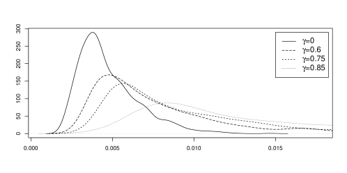
Figure 2: Smoothed histograms of DGP (Q2) for different values of $\gamma$.

References

• [1] Abadir, K.M., Distaso, W., Giraitis, L., Koul, H.L., 2014. Asymptotic normality for weighted sums of linear processes. Econometric Th., 30, 252–284.
• [2] Beran, J., Schützner, M., 2009. On approximate pseudo-maximum likelihood estimation for LARCH processes. Bernoulli, 15, 1057–1081.
• [3] Bollerslev, T., 1986. Generalized autoregressive conditional heteroscedasticity. J. Econometrics, 3, 307–327.
• [4] Burkholder, D.L., 1973. Distribution functions inequalities for martingales. Ann. Probab., 1, 19–42.
• [5] Doukhan, P., Grublytė, I., Surgailis, D., 2015. A nonlinear model for long memory conditional heteroscedasticity. Preprint. Available at arXiv: 1502.00095v2 [math.ST].
• [6] Engle, R.F., 1982. Autoregressive conditional heterosckedasticity with estimates of the variance of United Kingdom inflation. Econometrica, 50, 987–1008.
• [7] Engle, R.F., 1990. Stock volatility and the crash of ’87. Discussion. Rev. Financial Studies 3, 103–106.
• [8] Francq, C., Zakoian, J.-M., 2010. Inconsistency of the MLE and inference based on weighted LS for LARCH models. J. Econometrics 159, 151–165.
• [9] Giraitis, L., Robinson, P.M., Surgailis, D., 2000. A model for long memory conditional heteroskedasticity. Ann. Appl. Probab., 10, 1002–1024.
• [10] Giraitis, L., Leipus, R., Robinson, P.M., Surgailis, D., 2004. LARCH, leverage and long memory. J. Financial Econometrics, 2, 177-210.
• [11] Giraitis, L., Leipus, R., Surgailis, D., 2009. ARCH($\infty$) models and long memory properties. In: T.G. Andersen, R.A. Davis, J.-P. Kreiss, T. Mikosch (Eds.) Handbook of Financial Time Series, pp. 71–84. Springer-Verlag.
• [12] Giraitis, L., Surgailis, D., Škarnulis, A., 2014. Integrated AR and ARCH processes and the FIGARCH model: origins of long memory. Preprint.
• [13] Grublytė, I., Surgailis, D., Škarnulis, A., 2015. Quasi-MLE for quadratic ARCH model with long memory. Preprint. Available at arXiv:1509.06422 [math.ST].
• [14] Levine, M., Torres, S., Viens, F., 2009. Estimation for the long-memory parameter in LARCH models, and fractional Brownian motion. Stat. Inf. Stoch. Process. 12, 221–250.
• [15] Osȩkowski, A., 2012. A note on Burkholder-Rosenthal inequality. Bull. Polish Acad. Sci. Mathematics 60, 177–185.
• [16] Robinson, P.M., 1991. Testing for strong serial correlation and dynamic conditional heteroskedasticity in multiple regression. J. Econometrics, 47, 67–84.
• [17] Rosenthal, H.P., 1970. On the subspaces of $L^{p}(p>2)$ spanned by the sequences of independent random variables. Israel J. Math., 8, 273–303.
• [18] Sentana, E., 1995. Quadratic ARCH models. Rev. Econom. Stud. 3, 77–102.
• [19] Truquet, L., 2014. On a family of contrasts for parametric inference in degenerate ARCH models. Econometric Th., 30, 1165–1206.
• [20] von Bahr, B. and Esséen, C.-G., 1965. Inequalities for the $r$th absolute moment of a sum of random variables, $1\leq r\leq 2$. Ann. Math. Statist. 36, 299–303.