Josephson current in a normal-metal nanowire coupled to superconductor/ferromagnet/superconductor junction

Abstract

We consider superconducting nanowire proximity coupled to superconductor / ferromagnet / superconductor junction, where the magnetization penetrates into superconducting segment in nanowire decaying as $\sim\exp[-\frac{\mid n\mid}{\xi}]$, where $n$ is the site index and the $\xi$ is the decay length. We tune chemical potential and spin-orbit coupling so that topological superconducting regime hosting Majorana fermion is realized for long $\xi$. We find that when $\xi$ becomes shorter, zero energy state at the interface between superconductor and ferromagnet splits into two states at nonzero energy. Accordingly, the behavior of Josephson current is drastically changed due to this “zero mode-non-zero mode crossover”. By tuning the model parameters, we find an almost second-harmonic current-phase relation, $\sin 2\varphi$, where $\varphi$ is the phase difference of the junction. Based on the analysis of Andreev bound state (ABS), we clarify that the current-phase relation is determined by coupling of the states within the energy gap. We find that the emergence of crossing points of ABS is a key ingredient to generate $\sin 2\varphi$ dependence in the current-phase relation. We further study both the energy and $\varphi$ dependence of pair amplitudes in the ferromagnetic region. For large $\xi$, odd-frequency spin-triplet $s$-wave component is dominant. The magnitude of the odd-frequency pair amplitude is enhanced at the energy level of ABS.

I Introduction

It is known that a number of remarkable physical phenomena occur in superconductor/ferromagnet (S/F) hybrid structures. Golubov et al. (2004); Buzdin (2005); Bergeret et al. (2005a) First one is the generation of $\pi$-state Bulaevskii et al. (1977); Buzdin et al. (1982) in S/F/S junctions. Since the exchange coupling and spin-singlet Cooper pair are competing each other, spin-singlet pairs in ferromagnet have a spatial oscillation with changing sign in the presence of the exchange coupling. Fulde and Ferrell (1977); Larkin and Ovchinnikov (1965); Ryazanov et al. (2001); Kontos et al. (2002); Robinson et al. (2006) Next one is the dominant second-harmonic in the current-phase relation of Josephson current, $\sin 2\varphi$, where $\varphi$ is the phase difference across the junction. It is known that $\sin 2\varphi$ dependence Tan (1997) appears near the $0$-$\pi$ transition point.Sellier et al. (2004); Robinson et al. (2007) The third one is the generation of the odd-frequency pairing in the F region by proximity effect in S/F hybrid systems.Bergeret et al. (2001); Bergeret et al. (2005a); Volkov et al. (2003) There have been many theoretical Eschrig (2011); Eschrig et al. (2003) and experimental Keizer et al. (2006); Sosnin et al. (2006); Khaire et al. (2010); Robinson et al. (2010); Sprungmann et al. (2010); Anwar et al. (2010) works about proximity effect via odd-frequency pairing in S/F junctions. The fourth one is the so called inverse proximity effect where magnetization penetrates into a superconductor.Bergeret et al. (2004); Bergeret et al. (2005b); Linder et al. (2009); Xia et al. (2009) The electronic property and pairing symmetry near the S/F interface is drastically changed by this effect.

Independently of research directions mentioned above, study of nanowire on the surface of superconductor in the presence of applied Zeeman magnetic field has recently become a hot topic in condensed matter physics.Lutchyn et al. (2010); Oreg et al. (2010) Due to the strong spin-orbit coupling (SOC) in nanowire, topological superconducting state is generated. Then, by the bulk-edge correspondence, superconducting nanowire hosts Majorana fermion (MF) as the end state, Sato and Fujimoto (2009); Lutchyn et al. (2010); Oreg et al. (2010) which is one of important factors to realize quantum computation. Kitaev (2001); Alicea (2012); Alicea et al. (2011); Nayak et al. (2008) It has also been reported that a chain of ferromagnetic atoms on a superconductor forms a topologically non-trivial state, where the ABS within the superconducting gap is localized around the edge as a MF.Nadj-Perge et al. (2013, 2014); Pöyhönen et al. (2014); Pientka et al. (2014); Braunecker and Simon (2013); Klinovaja et al. (2013); Pawlak et al. (2015); Hoffman et al. (2015); Meng et al. (2015) The common feature in these one-dimensional topological superconducting systems is that both pair potential and magnetization coexist in all sites of the nanowire.

Up to now, although inverse proximity effect and topological superconductivity have been studied independently, they have not been studied simultaneously. It is a challenging issue to clarify a new effect where both effects coexist in the same model. If we consider proximity coupled nanowire on the S/F/S junction, we can divide the nanowire into the three segments; left superconductor, middle ferromagnet and right superconductor. Thus, it is possible to design effective one-dimensional S/F/S junctions in nanowire. We consider the situation where the ferromagnetic order of F depends on the position in the S/F/S junction. Besides, to discuss topological superconductivity, we consider Rashba-type SOC in nanowire. If $\xi$ which represents the penetration length of ferromagnetic order is long, zero energy state is generated at the S/F interface. On the other hand, if $\xi$ is short, we can expect that this zero energy state splits into two Yu (1965); H.Shiba (1968); Rusinov (1969) around the magnetic impurity. Thus, proximity coupled nanowire on the S/F/S junction is interesting since we can study both inverse proximity effect and topological superconductivity in the same model. If we tune $\xi$ as a parameter, the present model has a unique feature to study a new-type of inverse proximity effect including topological superconductivity.

In this paper, we study electronic spectra and resulting Josephson current in this nanowire S/F/S model. First, we calculate local density of states (LDOS) of isolated left side superconducting segment where magnetization penetrates from the right edge proportional to $\exp[\frac{n}{\xi}_{L}]$ with site index $n<0$ and the decay length $\xi_{L}$. We clarify that if $\xi_{L}$ exceeds a certain value, LDOS has a clear zero energy peak (ZEP) due to the zero mode at the edge. On the other hand, when $\xi_{L}$ becomes shorter, LDOS has a peak splitting. We call this effect as “zero mode-non-zero mode crossover”. Throughout this paper, we introduce zero mode and non-zero mode to distinguish zero energy state localized at the interface and splitted state. We study the Josephson current in the S/F/S nanowire junction by changing the decay length of ferromagnetic order into the left (right) side superconductor, $\xi_{L}$ ($\xi_{R}$), and chemical potential of ferromagnet. It is seen that the behavior of Josephson current is quite different when the decay length becomes shorter due to the “zero mode-non-zero mode crossover”.

Especially when this non-zero modes Yu (1965); H.Shiba (1968); Rusinov (1969) are localized at the boundary between superconductor and ferromagnet, we find an anomalous current-phase relation which can be roughly expressed as $\sin 2\varphi$. In order to understand the physical origin of the current-phase relation more clearly, we calculate the ABS and provide an argument that the emergence of crossing points of ABS is a key ingredient to produce current-phase relation $\sin 2\varphi$. We find that the emergence of crossing points of ABS is a key ingredient to generate $\sin 2\varphi$ dependence in current-phase relation. This mechanism is distinct from preexisting case in S/F/S junctions. Golubov et al. (2004); Tan (1997); Sellier et al. (2004); Robinson et al. (2007) We also calculate pair amplitude decomposing into odd-frequency part and even-frequency one. We focus on $s$-wave component of odd-frequency spin-triplet even-parity (OTE) pairing and show their dependence on energy and phase difference $\varphi$. For large magnitude of $\xi_{L(R)}$, equal spin OTE pair amplitude becomes dominant and enhanced at the energy level of the ABS.

This paper is organized as follows: In Sec. II, we provide the formulation to calculate LDOS and Josephson current using recursive Green’s function technique. In Sec. III.1, we calculate LDOS on the edge of isolated left side superconducting segment with decaying ferromagnetic order from the right edge. In Sec. III.2, we analyze the Josephson current in S/F/S junction changing decay length of ferromagnetic order parameter and chemical potential of ferromagnet. In Sec. III.3, we calculate ABS and discuss the relevance to current-phase relation in Sec. III.2. In Sec. III.4, we calculate pair amplitudes to shed light on these results from different angles. Finally, we summarize our results in Sec. IV.

II Formulation

In this section we provide a formulation to calculate LDOS and Josephson current using recursive Green’s function. The method of calculating ABS is also included in this section.

First, we review some general aspects of the recursive Green’s function technique. Its spirit is as follows: to build the full Green’s function, we start from isolated blocks and connect them to other parts of the system by stacking sites one by one along a certain direction. For example, we consider a one-dimensional atomic chain along $x$-direction as shown in Fig. 1(a) and suppose that the Green’s function of the detached $N$ sites on the left side has been known. We denote $G_{N,N}^{\text{L}}$ as the Green’s function at the $N$ site. Consider adding one more site from the right to this system. Based on Dyson equation, we have

$$G_{N+1,N+1}^{\text{L}}=g_{\text{iso}}+g_{\text{iso}}V_{N+1,N}G_{N,N+1}^{\text{L}}$$ (1)

$$G_{N,N+1}^{\text{L}}=G_{N,N}^{\text{L}}V_{N,N+1}G_{N+1,N+1}^{\text{L}},$$ (2)

where $g_{\text{iso}}$ is the Green’s function of the isolated $N+1$ site. Substituting Eq. (1) into Eq. (2), we get

$$G_{N+1,N+1}^{\text{L}}=\Bigl{[}g_{\text{iso}}^{-1}-V_{N+1,N}G_{N,N}^{\text{L}}V_{N,N+1}\Bigr{]}^{-1}.$$ (3)

LDOS can be calculated as follows:

$$\rho^{L}(E)=-\frac{1}{\pi}\text{ImTr}\Bigl{[}G_{N+1,N+1}^{\text{L}}(E+i0^{+})\Bigr{]},$$ (4)

with infinitesimal positive number $0^{+}$. Similarly, one can determine the Green’s function by stacking from right to left (in this case the superscript of $G$ is replaced with $R$, such as $G_{N,N}^{\text{R}}$). Provided that we start this stacking process simultaneously from the two ends, we can obtain the Green’s function $G_{N-1,N-1}^{\text{L}}$ at site $N-1$ of the left chain and $G_{N+2,N+2}^{\text{R}}$ at site $N+2$ of the right chain.

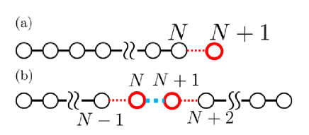
Figure 1: (a) A schematic picture of one-dimensional chain which is created by adding sites from left to right. (b) A schematic picture of one-dimensional chain which is created by stacking sites both from left to right and right to left and finally connect the two chains.

From Eq. (3), we know that the process of adding the site $N$ in the left chain generates

$$G_{N,N}^{\text{L}}=\Bigl{[}g_{\text{iso}}^{-1}-V_{N,N-1}G_{N-1,N-1}^{\text{L}}V_{N-1,N}\Bigr{]}^{-1},$$ (5)

and similarly

$$G_{N+1,N+1}^{\text{R}}=\Bigl{[}g_{\text{iso}}^{-1}-V_{N+1,N+2}G_{N+2,N+2}^{\text{R}}V_{N+2,N+1}\Bigr{]}^{-1},$$ (6)

from adding the site $N+1$ in the right chain. Now we connect the two chains (light-blue dashed line in Fig. 1(b)) and denote the Green’s function of this combined chain as $G$. Based on Dyson equation we get following equations:

$$G_{N,N}=\Bigl{[}G_{N,N}^{-1\text{L}}-V_{N,N+1}G_{N+1,N+1}^{\text{R}}V_{N+1,N}\Bigr{]}^{-1},$$ (7)

$$G_{N+1,N+1}=\Bigl{[}G_{N+1,N+1}^{-1\text{R}}-V_{N+1,N}G_{N,N}^{\text{L}}V_{N,N+1}\Bigr{]}^{-1}$$ (8)

$$G_{N,N+1}=G_{N,N}^{\text{L}}V_{N,N+1}G_{N+1,N+1}$$ (9)

$$G_{N+1,N}=G_{N+1,N+1}^{\text{R}}V_{N+1,N}G_{N,N}.$$ (10)

Suppose hopping amplitude of adjacent sites is given by $t$, we can calculate the current

$$J=-ietk_{B}T\sum_{\omega_{n}}\text{Tr}\Bigl{[}G_{N+1,N}(\omega_{n})-G_{N,N+1}(\omega_{n})\Bigr{]},$$ (11)

with Boltzman constant $k_{B}$, temperature $T$, and Matsubara frequency $\omega_{n}$.

Next, we construct the model Hamiltonian of the semiconducting nanowire on top of the S/F/S junction (Fig. 2(a)). We separate this nanowire into three parts by introducing

$$S_{1} = \bigl{\{}n|1\leq n\leq L_{\text{SC}}\bigr{\}}$$

$$S_{2} = \{n|L_{\text{SC}}+1\leq n\leq L_{\text{SC}}+L_{\text{FM}}\}$$

$$S_{3} = \{n|L_{\text{SC}}+L_{\text{FM}}+1\leq n\leq 2L_{\text{SC}}+L_{\text{FM}}\}$$ (12)

with site index $n$. We denote the equal site length of each side of superconductors as $L_{\text{SC}}$ and that of ferromagnet as $L_{\text{FM}}$. We define Hamiltonian as follows:

$$\mathcal{H}=-t\sum_{\begin{subarray}{c}\left\langle m,n\right\rangle\\ \sigma\end{subarray}}c_{m\sigma}^{\dagger}c_{n\sigma}+\sum_{\begin{subarray}{c}n\in S_{1}\\ n\in S_{3}\end{subarray}}(\frac{A}{2}c_{n\uparrow}^{\dagger}c_{n+1\downarrow}-\frac{A}{2}c_{n\downarrow}^{\dagger}c_{n+1\uparrow}+\text{H.c.})-\sum_{\begin{subarray}{c}n\in S_{1}\\ \sigma\end{subarray}}\mu c_{n\sigma}^{\dagger}c_{n\sigma}+\sum_{n\in S_{1}}(\Delta c_{n\uparrow}^{\dagger}c_{n\downarrow}^{\dagger}+\text{H.c.})$$

$$-\sum_{\begin{subarray}{c}n\in S_{3}\\ \sigma\end{subarray}}\mu c_{n\sigma}^{\dagger}c_{n\sigma}+\sum_{n\in S_{3}}(\Delta e^{i\varphi}c_{n\uparrow}^{\dagger}c_{n\downarrow}^{\dagger}+\text{H.c.})-\sum_{\begin{subarray}{c}n\in S_{2}\\ \sigma\end{subarray}}\mu_{\text{FM}}c_{n\sigma}^{\dagger}c_{n\sigma}+\sum_{n\in S_{2}}V_{z}(c_{n\uparrow}^{\dagger}c_{n\uparrow}-c_{n\downarrow}^{\dagger}c_{n\downarrow})$$

$$+\sum_{n\in S_{1}}V_{z}\exp\Bigl{[}\frac{n-L_{\text{SC}}}{\xi_{L}}\Bigr{]}(c_{n\uparrow}^{\dagger}c_{n\uparrow}-c_{n\downarrow}^{\dagger}c_{n\downarrow})+\sum_{n\in S_{3}}V_{z}\exp\Bigl{[}\frac{L_{\text{SC}}+L_{\text{FM}}+1-n}{\xi_{R}}\Bigr{]}(c_{n\uparrow}^{\dagger}c_{n\uparrow}-c_{n\downarrow}^{\dagger}c_{n\downarrow})$$ (13)

where $c_{n\sigma}^{\dagger}(c_{n\sigma})$ is the electron creation (annihilation) operator with site $n$ and spin $\sigma$, $t$ is the hopping matrix between the nearest neighbor $\left\langle i,j\right\rangle$, $A$ is the Rashba spin orbit coupling (SOC), $\mu(\mu_{\text{FM}})$ is chemical potential in superconductor (ferromagnet) segment, $\Delta$ is the pair potential, $\varphi$ is the phase difference of superconductors, $V_{z}$ is the ferromagnetic order, and $\xi_{R(L)}$ is the decay length of ferromagnetic order in the right (left) superconductor. Unlike the model Hamiltonian on top of the superconductor with uniform ferromagnetic order, in this model construction, we assume that ferromagnetic order penetrates into right (left) superconductor segment decaying as $\sim\exp[\frac{-n}{\xi_{R}}](\exp[\frac{n}{\xi_{L}}])$ as described in Eq. (13). As for Rashba SOC, we do not include the second term in Eq. (13) at the interface between superconductor and ferromagnet since it does not affect our results.

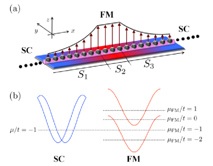
Figure 2: (a) A schematic picture of a nanowire on top of S/F/S junction. (b) Chemical potential of a nanowire in the superconductor segment (left) and ferromagnet segment (right).

Now we apply the recursive Green’s function technique to calculate LDOS, Josephson current and ABS. The retarded and Matsubara Green’s function of the isolated site can be described as

$$g_{\text{iso}}(E)=\frac{1}{(E+i0^{+})-\mathcal{H}_{\text{iso}}}$$ (14)

$$g_{\text{iso}}(\omega_{n})=\frac{1}{i\omega_{n}-\mathcal{H}_{\text{iso}}}$$ (15)

where $\mathcal{H}_{\text{iso}}$ is

$$\mathcal{H}_{\text{iso}}=c_{n}^{\dagger}\hat{\mathcal{H}}_{\text{iso}}c_{n}$$

$$\hat{\mathcal{H}}_{\text{iso}}=\begin{cases}-\mu\sigma_{0}\tau_{z}-\sigma_{y}\tau_{y}\Delta,\;\;n\in S_{1}\\ -\mu_{\text{FM}}\sigma_{0}\tau_{z},\;\;n\in S_{2}\\ -\mu\sigma_{0}\tau_{z}-\sigma_{y}\tau_{\downarrow}\Delta e^{i\varphi}-\sigma_{y}\tau_{\uparrow}\Delta e^{-i\varphi},\;\;n\in S_{3}\end{cases}$$ (16)

with the basis $c_{n}=(c_{n\uparrow},c_{n\downarrow},c_{n\uparrow}^{\dagger},c_{n\downarrow}^{\dagger})$. $\sigma_{0,x,y,z}(\tau_{0,x,y,z})$ is Pauli matrix in spin (particle-hole) space and $\tau_{\uparrow}=(\tau_{x}+i\tau_{y})/2$, $\tau_{\downarrow}=(\tau_{x}-i\tau_{y})/2$. Hopping matrix can be written as follows:

$$V_{n,n+1} = c_{n}^{\dagger}\hat{V}_{n,n+1}c_{n+1}$$

$$V_{n+1,n} = c_{n+1}^{\dagger}\hat{V}_{n+1,n}c_{n},$$

$$\hat{V}_{n,n+1}=\begin{cases}-t\sigma_{0}\tau_{z}-i\frac{A}{2}\tau_{z}\sigma_{y},\;\;n\in S_{1},n\in S_{3}\\ -t\sigma_{0}\tau_{z},\;\;n\in S_{2}\end{cases}$$ (17)

$$\hat{V}_{n+1,n}=\begin{cases}-t\sigma_{0}\tau_{z}+i\frac{A}{2}\tau_{z}\sigma_{y},\;\;n\in S_{1},n\in S_{3}\\ -t\sigma_{0}\tau_{z},\;\;n\in S_{2}\end{cases}$$ (18)

In the next section, we will calculate the LDOS on the edge of the nanowire with proximity coupled pair potential and decaying ferromagnetic order, Josephson current and ABS of the nanowire on S/F/S junction. LDOS is given by

$$\rho^{L}(E)=-\frac{1}{\pi}\text{ImTr}\Bigl{[}G_{L_{\text{SC}},L_{\text{SC}}}^{L}(E+i0^{+})\Bigr{]}.$$ (19)

From Eq. (24), Josephson current and ABS are described as follows:

$$J(\varphi)=-ietk_{B}T\sum_{\omega_{n}}\text{Tr}\Bigl{[}G_{n+1,n}(\omega_{n})-G_{n,n+1}(\omega_{n})\Bigr{]},\;\;n\in S_{2}$$ (20)

$$\rho(E,\varphi)=-\frac{1}{\pi}\text{ImTr}\Bigl{[}G_{n,n}(E+i0^{+})\Bigr{]},\;\;n\in S_{2}$$ (21)

where $\varphi$ is the macroscopic phase difference of pair potential between two superconductors. We can calculate $\varphi$ dependence explicitly.

III Results

This section consists of four parts: in subsection A, we study the LDOS on the edge of the nanowire with both pair potential and decaying ferromagnetic order and exhibit the evolution of the surface resonance modes. In subsection B, we then calculate Josephson current S/F/S junctions of the nanowire with several different decay length. It shows that at specific parameter tuning, anomalous current-phase relation which can be roughly regarded as $\sin 2\varphi$ appears. In subsection C, we calculate ABS. From the spectrum of ABS, we will provide a simple argument of explanation that the emergence of crossing points of ABS is the important factor to realize the current-phase relation $\sin 2\varphi$. In subsection D, we finally analyze the symmetry of pair amplitudes in this junction especially focusing on odd-frequency pairing. Odd-frequency spin-triplet pairing is enhanced when the Majorana like zero energy state is generated at the S/F (F/S) interface.Asano and Tanaka (2013) Throughout this section, we fix the parameters as follows: $\Delta/t=0.1,\mu/t=-1,A/t=1,V_{z}/t=1.5$. With this choice of parameters, condition of topological non-trivial stateOreg et al. (2010) is satisfied when ferromagnetic order is uniform. We set the number of sites of superconductor segment long enough so that the effect of overlapping between two zero energy modes on the edges of segment is negligible. In actual numerical calculation, we fix the number of sites of superconductor segment as $L_{\text{SC}}=4000$ and ferromagnet one as $L_{\text{FM}}=4$. To calculate retarded Green’s function, we set the infinitesimal positive number $0^{+}$ as $0^{+}/t=0.001$.

III.1 LDOS

In this subsection, we examine the LDOS on the edge of nanowire which is calculated from Eq. (19). The situation is illustrated in Fig. 3(a), where the pair potential and decaying ferromagnetic order coexist.

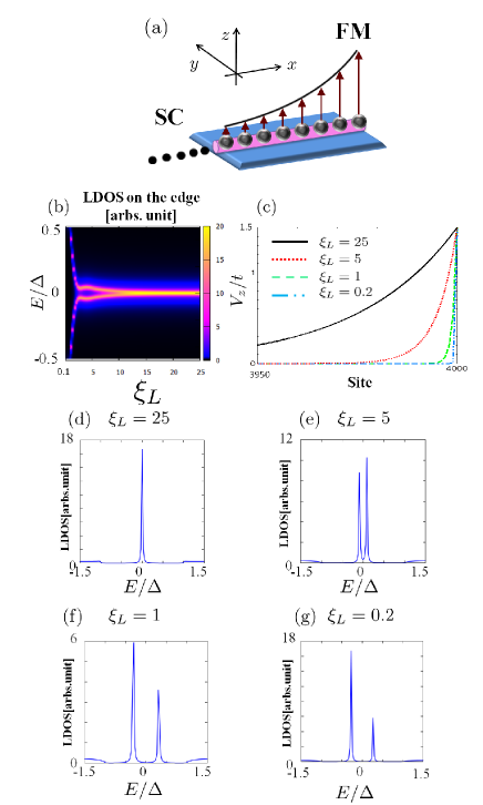
Figure 3: (a) A schematic picture of a nanowire on top of superconductor with decaying ferromagnetic order. (b) The intensity plot of LDOS on the edge ($i.e.$ $n=L_{\text{SC}}$) of the nanowire shown in (a). (c) The spatial profiles of ferromagnetic order with different decay length, $\xi_{L}=25$ (black solid line), $\xi_{L}=5$ (red dotted line), $\xi_{L}=1$ (green dashed line), and $\xi_{L}=0.2$ (blue 2 dotted line). (d)-(g) LDOS on the edge of the nanowire with different decay length.

The intensity of LDOS is plotted in Fig. 3(b). It is shown that for the long decaying of $V_{z}$ $\left(\xi_{L}>10\right)$, there is a single resonance peak at zero energy. This is in agreement with the finding that in the asymptotic scenario when $V_{z}$ is spatially uniform at infinite $\xi_{L}$, such nanowire is topologically non-trivial which can be confirmed by the sign of Pfaffian with our choice of parameters.Kitaev (2001) However, in the presence of spatially nonuniform ferromagnetic order, the preexisting topological argument is no longer valid. Thus, it is remarkable to see here that even if the ferromagnetic order is non-uniform, LDOS with zero energy peak can still appear on the edge of the nanowire within the numerical accuracy. On the opposite, with the decay length less than around $\xi_{L}\sim 10$, this zero mode splits into two resonance peaks symmetric to zero energy. Owing to the localized ferromagnet at the end of nanowire, this finding associates with another important physical results known as Shiba states.Yu (1965); H.Shiba (1968); Rusinov (1969) It is well known that when a magnetic impurity is put on the superconductor, there is a bound state around the impurity inside the superconducting energy gap. In the present model, we can control the “zero mode-non-zero mode crossover” with decreasing the decay length of ferromagnetic order. In Figs. 3(d)-(g), we plot the LDOS for a selected decay length $\xi_{L}=25,5,1,$ and $0.2$ respectively (see also Fig. 3(c) where the spatial profiles of ferromagnetic order are shown for four different decay length). When $\xi_{L}=25$, we see the zero energy mode, on the other hand, in the rest of the cases (Figs. 3(e)-(g)), we find non-zero modes in the energy gap of superconducting region.

In Appendix A, we consider the overlapping of two zero energy modes in the shorter length system and also compare non-uniform ferromagnetic case and uniform case, which leads that two zero energy modes appeared in non-uniform situation can be regarded as two MFs.

III.2 Josephson current

In this subsection, we study Josephson currents for various decay lengths of ferromagnetic order on both sides of the superconductor. On the left side, we are interested in three typical decay lengths $\xi_{L}=25,1,$ and $0$ ($i.e.$, ferromagnetic order does not penetrate into the left superconductor). In each case, we will tune the decay length $\xi_{R}$ as well as the chemical potential of the ferromagnet segment ($\mu_{\text{FM}}/t=-2,-1,0,$ and $1$, see also Fig. 2(b)).

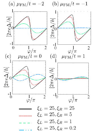
Figure 4: (a)-(d) Josephson current of the nanowire on top of S/F/S junction in the case of $\xi_{L}=25$ with four different chemical potentials of ferromagnetic layer listed above each figure. There are four lines in each figure: $\xi_{L}=25,\xi_{R}=25$ (black solid line), $\xi_{L}=25,\xi_{R}=5$ (red dashed line), $\xi_{L}=25,\xi_{R}=1$ (green dashed line), and $\xi_{L}=25,\xi_{R}=25$ (blue 2 dotted line).

First, we look at the case $\xi_{L}=25$. As the previous discussion shows, there is zero energy mode on the edge of the left nanowire. In Figs. 4(a)-(d), we plot Josephson currents for $\mu_{\text{FM}}/t=-2,-1,0,$ and $1$, respectively. In each figure, we take four values of $\xi_{R}$: $25$, $5$, $1$ and $0.2$. The phase dependence of the current in all cases has the dominant coupling proportional to $\sin\varphi$. Interestingly, for $\mu_{\text{FM}}/t=-2,-1$ and $0$, the Josephson current in symmetric junctions abruptly changes its sign at $\varphi=\pi$ as shown in Figs. 4(a), (b) and (c), respectively. In asymmetric junctions, such jump is absent. Notice that our system considered here has no perfect transmissivity and is closely similar to that of two $d$-wave superconductor with zero energy ABSs,Tanaka and Kashiwaya (1997a); Tanaka and Kashiwaya (1996a); Kashiwaya and Tanaka (2000) $p$-wave superconductors Kwon et al. (2004a); Asano et al. (2006a) or Kitaev chains junction system where MFs are coupled each other.Kitaev (2001); Law and Lee (2011) Therefore, the abrupt jump can only be explained by the existence of robust zero energy ABSs,Buchholtz and Zwicknagl (1981); Hara and Nagai (1986); Hu (1994); Tanaka and Kashiwaya (1995, 1996b) $i.e.$, MFs.Kitaev (2001) However, in the non-uniform ferromagnetic order, the formation of zero modes are distinct from $p$-wave superconductor or Kitaev model. It is interesting that the similar behavior of Josephson current is found even in the present model. For $\mu_{\text{FM}}/t=1$, we obtain $\pi$-state and the current are quite small compared to the other cases of chemical potentials. In this case, there is one band at the chemical potential in ferromagnetic region which has opposite spin compared to the ferromagnetic order in SCs. Thus, the transparency of the junction is greatly reduced and $\pi$-state can appear as a result of misaligned magnetizations.

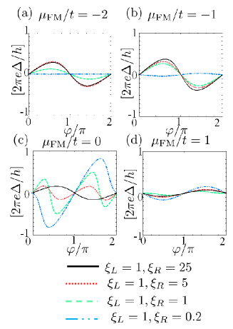
Figure 5: (a)-(d) Josephson current of the nanowire on top of S/F/S junction in the case of $\xi_{L}=1$ with four different chemical potentials of ferromagnetic layer listed in above each figure. There are four lines in each figure: $\xi_{L}=1,\xi_{R}=25$ (black solid line), $\xi_{L}=1,\xi_{R}=5$ (red dashed line), $\xi_{L}=1,\xi_{R}=1$ (green dashed line), and $\xi_{L}=1,\xi_{R}=0.2$ (blue 2 dotted line).

Second, we focus on the case $\xi_{L}=1$ where non-zero modes are localized on the left segment. As for $\mu_{\text{FM}}/t=-2$ and $-1$ (Figs. 5(a) and (b)), we find the current-phase relation $\sin\varphi$ in three cases: $\xi_{R}=25$ (black solid line), $\xi_{R}=5$ (red dotted line), and $\xi_{R}=1$ (green dashed line). On the other hand Josephson current is almost zero when $\xi_{R}=0.2$ (blue 2 dashed line). Surprisingly, when $\mu_{\text{FM}}/t=-2$, $\xi_{R}=5$ and $\xi_{R}=1$ (Fig. 5(c) red dotted and green dashed lines), we find the anomalous current-phase relation which can be roughly regarded as $\sin 2\varphi$. As we will see in the next subsections, the coupling of non-zero modes produces this anomalous current-phase relation especially when the emergence of crossing points of ABS becomes the important factor. For $\mu_{\text{FM}}/t=1$, all of the Josephson currents are suppressed compared to the other cases of chemical potential.

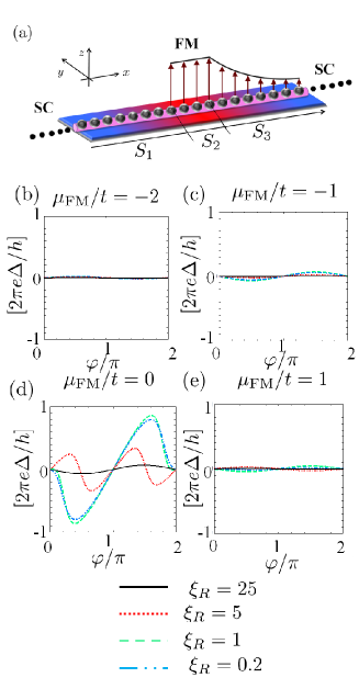
Figure 6: (a) A schematic picture of a nanowire on top of S/F/S junction. (a)-(d) Josephson current of the nanowire on top of S/F/S junction in the case of $\xi_{L}=0$, that is, ferromagnetic order does not penetrate into left superconductor segment. Results are shown with four different chemical potentials of ferromagnetic layer listed above each figure. There are four lines in each figure: $\xi_{L}=0,\xi_{R}=25$ (black solid line), $\xi_{L}=0,\xi_{R}=5$ (red dashed line), $\xi_{L}=0,\xi_{R}=1$ (green dashed line), and $\xi_{L}=0,\xi_{R}=25$ (blue 2 dotted line).

Finally, we study the case $\xi_{L}=0$, $i.e.$, the ferromagnetic order does not penetrate into the left superconductor segment. When $\mu_{\text{FM}}/t=-2,-1$ and $1$ (Figs. 6(b), (c), and (d), respectively), Josephson current is almost zero, on the other hand, when $\mu_{\text{FM}}/t=0$, we see current-phase relation $\sin 2\varphi$ with decay length on the right $\xi_{R}=5$ (dotted red line) and $-\sin\varphi$ with other decay length.

Before we proceed, it is instructive to summarize the interesting phenomena we have found in this subsection. In the case of $\xi_{L}=25$ and $\mu_{\text{FM}}/t=-2,-1,0$, we see the abrupt sign reversal of current at $\varphi=\pi$. In the case of $\xi_{L}=25$ and $\mu_{\text{FM}}/t=1$, the amplitude of Josephson current is suppressed. When $\xi_{L}=1$, $\mu_{\text{FM}}/t=0$, and $\xi_{R}=5$ or $1$, we obtain current-phase relation approximated as $\sin 2\varphi$. We also find this current-phase relation $\sin 2\varphi$ in the case of $\xi_{L}=0$, $\mu_{\text{FM}}/t=0$, and $\xi_{R}=5$.

III.3 ABS

In this subsection, we study the ABS of nanowire on S/F/S junction with different decay length and relate it to the behavior of Josephson current obtained in the previous subsection. We mainly focus on the case of $\mu_{\text{FM}}/t=0$. It is well known that when the magnitudes of the pair potential are the same on the left and right side of superconductor, Josephson current can be calculated by:

$$J(\varphi)=\frac{2e}{h}\frac{\partial F(\varphi)}{\partial\varphi},$$ (22)

where $F$ is free energy. In one dimension, $F$ can be written as

$$F=-k_{B}T\sum_{n}\log\Bigl{(}2\cosh\bigl{(}\frac{\varepsilon_{n}}{2k_{B}T}\bigr{)}\Bigr{)}$$ (23)

where $\varepsilon_{n}$ is the energy of ABS Beenakker (2013). Therefore, Josephson current is

$$J(\varphi)=-\frac{2e}{h}k_{B}T\sum_{n}\frac{1}{\cosh\bigl{(}\frac{\varepsilon_{n}}{2k_{B}T}\bigr{)}}\sinh\bigl{(}\frac{\varepsilon_{n}}{2k_{B}T}\bigr{)}\frac{1}{2k_{B}T}\frac{\partial\varepsilon_{n}}{\partial\varphi}$$

$$=-\sum_{n}\frac{e}{h}\tanh\bigl{(}\frac{\varepsilon_{n}}{2k_{B}T}\bigr{)}\frac{\partial\varepsilon_{n}}{\partial\varphi}$$ (24)

At low temperature, $J(\varphi)$ can be approximated as

$$J(\varphi)\sim-\frac{e}{h}\sum_{n}\text{sgn}(\varepsilon_{n})\frac{\partial\varepsilon_{n}}{\partial\varphi}.$$ (25)

sgn$(\varepsilon_{n})$ gives $+1(-1)$ when $\varepsilon_{n}$ is positive (negative). In the above, $n$ denotes the band index of ABS. Due to the particle-hole symmetry, we can only take the ABSs below the zero energy into account. Thus, Josephson current can be approximated as the derivative of ABSs below the zero energy.

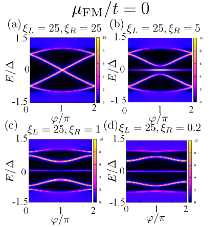
Figure 7: (a)-(d) ABS (the intensity plot of LDOS at the ferromagnet segment within the superconducting energy gap) in the case of $\mu_{\text{FM}}/t=0$ and $\xi_{L}=25$ with different decay length $\xi_{R}$.

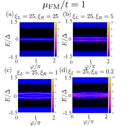
Figure 8: (a)-(d) ABS (the intensity plot of LDOS at the ferromagnet segment within the superconducting energy gap) in the case of $\mu_{\text{FM}}/t=1$ and $\xi_{L}=25$ with different decay length $\xi_{R}$.

First, we look at the case $\xi_{L}=\xi_{R}=25$ where the zero energy modes are located on both sides. These two zero modes hybridize as indicated in Fig. 7(a). The crossing point at $\varphi=\pi$ explains the sudden drop of Josephson current which can lead to the unusual $4\pi$ periodicity of current-phase relation if we consider AC Josephson current. As the decay length on the right decreases, the zero energy mode on the left does not hybridize with the states on the right, which can be seen from the flat ABS as a function of $\varphi$ in Figs. 7(b)-(d). The contribution of Josephson current is mainly carried by the ABSs away from zero energy. With this estimation, we can relate ABS to the behavior of Josephson current in the previous subsection. If we look at Figs. 7(b) and (c) ((d)), ABSs below the zero energy change as $\sim-\cos\varphi$ ($\sim\cos\varphi$) which leads to current-phase relation $\sin\varphi$ ($-\sin\varphi$). This consideration corresponds well to the black solid line and red dotted line (green dashed line) in Fig. 4(c). If we tune the chemical potential of ferromagnetic layer as $\mu_{\text{FM}}/t=1$, the ABSs are almost flat which do not make contribution to the Josephson current (Fig. 8). Indeed, the amplitude of Josephson currents are almost zero as shown in Fig. 4(d).

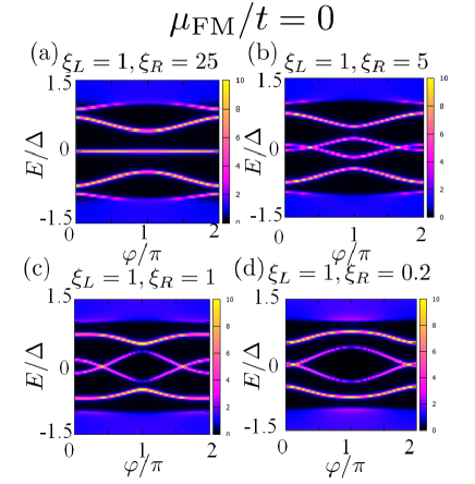
Figure 9: (a)-(d) ABS (the intensity plot of LDOS at the ferromagnet segment within the superconducting energy gap) in the case of $\mu_{\text{FM}}/t=0$ and $\xi_{L}=1$ with different decay length $\xi_{R}$.

Next, we focus on the case $\xi_{L}=1$, when non-zero modes are localized at the interface between left superconductor and ferromagnet segment. When decay length $\xi_{R}=25$ (Fig. 9(a)), the zero energy mode is located on the right segment. This mode is not coupled with the left non-zero modes. The major change of ABSs below the zero energy can be regarded as $\sim-\cos\varphi$ (Fig. 9(a)) which contributes $\sin\varphi$ to the Josephson current (Fig. 5(c) black solid line).

In the case of $\xi_{R}=5$ and $\xi_{R}=1$, when the anomalous current-phase relation $\sin 2\varphi$ can be seen, we find that non-zero modes on the both sides hybridize and these states are crossed at two values of $\varphi$: one is located at between $\varphi=0$ and $\pi$, another is between $\varphi=\pi$ and $\varphi=2\pi$ (Figs. 9(b) and (c)). As we discuss later, this crossing points of ABS is important to realize current-phase relation $\sin 2\varphi$. For $\xi_{R}=0.2$, all of the ABSs change as $\cos\varphi$ (Fig. 9(d)) which gives current-phase relation $\sin\varphi$ (Fig. 5(c) blue 2 dotted line).

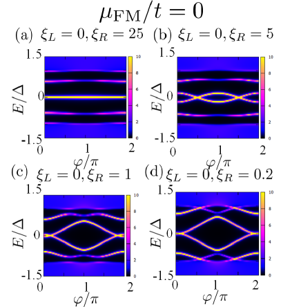
Figure 10: (a)-(d) ABS (the intensity plot of LDOS at the ferromagnet segment within the superconducting energy gap) in the case of $\mu_{\text{FM}}/t=0$ and $\xi_{L}=0$ ($i.e.$ there is no ferromagnetic order in the left superconductor segment.) with different decay length $\xi_{R}$.

Finally, we focus on the case $\xi_{L}=0$, $i.e.$, ferromagnetic order is absent in the left superconductor side (Fig. 10). If we set $\xi_{R}=25$, all of the ABSs becomes flat as a function of $\varphi$ which leads to almost zero Josephson current (Fig. 6(c) black solid line). For $\xi_{R}=1,0.2$, the change of ABS below the zero energy obeys $\sim\cos\varphi$ (Figs. 10(c) and (d)), thus, current-phase relation is $-\sin\varphi$ (Fig. 6(c) green dashed line and blue 2 dotted line). On the other hand, in the case of $\xi_{R}=5$, when we see current-phase relation $\sin 2\varphi$, we again find two crossing points of ABS (Fig. 10(b)).

From these analysis explained above, we find that the behavior of Josephson current can be determined by the hybridization of ABSs and when this hybridization produces the two crossing points at the zero energy, current-phase relation $\sin 2\varphi$ can be seen. Now we consider the simplified situation where there are two crossing points of ABSs: we have only two states within the energy gap (blue area in Fig. 11 top) which are labeled by $\varepsilon_{A}$ and $\varepsilon_{B}$ (Fig. 11 top). We assume $\varepsilon_{A}$ ($\varepsilon_{B}$) is written as $\sim-\cos\varphi$ ($\cos\varphi$) and crossing points are located at $\varphi=\frac{\pi}{2}$ and $\frac{3\pi}{2}$. According to Eq. (25) and particle-hole symmetry, we can focus on the states below the zero energy to estimate Josephson current. We separate the region of $\varphi$ into three: I $\{\varphi|0\leq\varphi<\frac{\pi}{2}\}$, II $\{\varphi|\frac{\pi}{2}\leq\varphi<\frac{3\pi}{2}\}$, III $\{\varphi|\frac{3\pi}{2}\leq\varphi<2\pi\}$ (Fig. 11 top). In I and III, ABS below the zero energy obeys $-\cos\varphi$, thus, Josephson current reads $\sim\sin\varphi$, while in II, ABS transforms into $\sin\varphi$ which gives Josephson current $-\sin\varphi$. We plot Josephson current as a function of $\varphi$ ($0\leq\varphi<2\pi$) in bottom of Fig. 11. Due to the different curve that ABS obeys in I and II (II and III), there is a jump at the boundary between I and II (II and III) which generates current-phase relation $\sin 2\varphi$. Up to now, $\sin 2\varphi$ dependence of Josepshon current has been discussed in S/ferromagnetic insulator/S junction,Tan (1997) S/F/S with diffusive F near the vicinity of $0-\pi$ transition point, Golubov et al. (2004); Sellier et al. (2004); Robinson et al. (2007) $d$-wave superconductor junctionsYip (1993); Tanaka and Kashiwaya (1996a, 1997b); Barash et al. (1996) and $s$-wave/spin triplet $p$-wave superconductor junctions.Yip (1993); Kwon et al. (2004b) Our setup of realizing $\sin 2\varphi$ dependence is distinct from the preexisting cases.

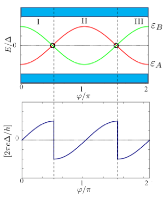
Figure 11: (top) A schematic picture of two ABSs denoted by as $\varepsilon_{A}$ (red) and $\varepsilon_{B}$ (green). These two states have two crossing points (solid circle) at $E=0$. (bottom) Josephson current which is given by $J(\varphi)\sim-\frac{\partial\varepsilon_{A}}{\partial\varphi}\text{sgn}(\varepsilon_{A})$

III.4 Symmetries of Cooper pair

In this subsection, we focus on the symmetry of Cooper pair in the present one-dimensional S/F/S junctions. In odd-frequency pairing state, the pair amplitude changes its sign with the exchange of times of two paired electrons.Berezinskii (1974) Taking account of this symmetry class, symmetry of Cooper pair is classified into (1) even-frequency spin-singlet even-parity (ESE), (2) even-frequency spin-triplet odd-parity (ETO), (3) odd-frequency spin-triplet even-parity (OTE), Berezinskii (1974) and (4) odd-frequency spin-singlet odd-parity (OSO). Black-Schaffer and Balatsky (2013) Although odd-frequency bulk superconductor has not been discovered up to now, odd-frequency pair amplitude can exist ubiquitously as a subdominant state. It is known that odd-frequency pairing is induced by the breaking of the translational Tanaka et al. (2007a, 2012); Eschrig et al. (2007) or spin-rotational symmetry Bergeret et al. (2001); Bergeret et al. (2005a); Volkov et al. (2003) from bulk even-frequency pair potential. Also, it has been clarified that zero-energy local density of states are enhanced by the odd-frequency pairing. Tanaka et al. (2007a, 2012); Asano et al. (2007a); Braude and Nazarov (2007); Asano et al. (2007b); Eschrig and Löfwander (2008) Odd-frequency pairing influences seriously the proximity effect and various electronic properties of the junctions.

In the present nanowire S/F/S junctions, the symmetry of pair amplitude far from the S/F (F/S) interface is ESE $s$-wave one, since the induced pair potential is conventional spin-singlet $s$-wave. Due to the symmetry breaking, near the S/F (F/S) interface or inside ferromagnet region, odd-frequency pairings can be induced. Here, we focus on $s$-wave component of ESE and OTE pair amplitudes in ferromagnet region. First we focus on the real frequency representation of pair amplitudes. ESE and OTE amplitudes are given by

$$f_{even}(E)=\frac{1}{2}\bigl{\{}F_{n,n}^{\uparrow,\downarrow}(E+i0^{+})+F_{n,n}^{\uparrow,\downarrow}(-E-i0^{+})\bigr{\}}$$ (26)

$$f_{odd}^{\sigma,\sigma^{\prime}}(E)=\frac{1}{2}\bigl{\{}F_{n,n}^{\sigma,\sigma^{\prime}}(E+i0^{+})-F_{n,n}^{\sigma,\sigma^{\prime}}(-E-i0^{+})\bigr{\}}$$ (27)

with $n\in S_{2}$. $F_{n,n}^{\sigma,\sigma^{\prime}}$ comes from Eq. (7):

$$G_{n,n}=\left(\begin{array}[]{cc}G&F\\ \tilde{F}&\tilde{G}\\ \end{array}\right),\;F=\left(\begin{array}[]{cc}F_{n,n}^{\uparrow,\uparrow}&F_{n,n}^{\uparrow,\downarrow}\\ F_{n,n}^{\downarrow,\uparrow}&F_{n,n}^{\downarrow,\downarrow}\\ \end{array}\right)$$ (28)

Above representation is useful to compare with the ABS. To clarify the relation between the ABS and the pair amplitude is an interesting issue, since it has been revealed that there is a close relation between ABS and odd-frequency pairing. In the presence of zero energy ABS as a surface state of unconventional superconductors, odd-frequency pair amplitude is hugely enhanced.Tanaka et al. (2007a, b, 2012); Bakurskiy et al. (2014) Thus the presence of zero energy state (ZES) can be interpreted as an emergence of odd-frequency pairing. Also, it has been clarified that MF always accompanies odd-frequency pairing. Asano and Tanaka (2013); Wakatsuki et al. (2014); Ebisu et al. (2015); Liu et al. (2015)

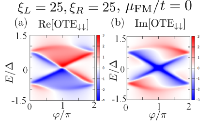
Figure 12: (a)(b):The intensity plot of real part (a) and imaginary part (b) of odd-frequency spin-triplet even-parity (OTE) pair amplitude with $\downarrow\downarrow$ spin component $f_{odd}^{\downarrow,\downarrow}(E)$ in the case of $\xi_{L}=25$, $\xi_{R}=25$, $\mu_{\text{FM}}/t=0$.

First, we calculate pair amplitude for $\xi_{L}=25$, $\xi_{R}=25$ and $\mu_{\text{FM}}/t=0$. The corresponding ABS with the hybridization of Majorana like ZESs in left and right side has been shown in Fig. 7(a). In this case, OTE pairing becomes dominant for any phase difference. As compared to other components, $f_{odd}^{\uparrow,\uparrow}(E)$, $f_{odd}^{\uparrow,\downarrow}(E)$ and $f_{even}(E)$, the magnitude of $f_{odd}^{\downarrow,\downarrow}(E)$ is dominant. This is because that the direction of the majority spin in ferromagnet is down. Therefore, we plot $s$-wave OTE pairing $f_{odd}^{\downarrow,\downarrow}(E)$ in the middle of the ferromagnet in Fig. 12. The energy and $\varphi$ dependence of $f_{odd}^{\downarrow,\downarrow}(E)$ is almost similar to those of ABS in Fig. 7. For $\varphi=0$, $\pi$ and $2\pi$, $\mathrm{Re}[f_{odd}^{\downarrow,\downarrow}(E)]=-\mathrm{Re}[f_{odd}^{\downarrow,\downarrow}(-E)]$ and $\mathrm{Im}[f_{odd}^{\downarrow,\downarrow}(E)]=\mathrm{Im}[f_{odd}^{\downarrow,\downarrow}(-E)]$. These relations of odd-frequency pairing are known in the previous study in normal metal / superconductor junctions.Tanaka and Golubov (2007)

Next, we look at the case with $\xi_{L}=\xi_{R}=1$ and $\mu_{FM}=0$. The corresponding ABS with double crossing points in the energy spectrum of ABS has been shown in Fig. 9(c). Such characteristic also appears in the intensity plot of $f_{odd}^{\downarrow,\downarrow}(E)$, $f_{odd}^{\uparrow,\downarrow}(E)$ and $f_{even}(E)$. The $E$ and $\varphi$ dependences of $f_{odd}^{\uparrow,\uparrow}(E)$ are similar to those of $f_{odd}^{\downarrow,\downarrow}(E)$. The remarkable point here is that not only odd-frequency pair amplitude but also even-frequency pair amplitude exists with the same order in contrast to the case in Fig. 13. For $\varphi=0$, $\pi$ and $2\pi$, $\mathrm{Re}[f_{odd}^{\sigma,\sigma^{\prime}}(E)]=-\mathrm{Re}[f_{odd}^{\sigma,\sigma^{\prime}}(-E)]$ and $\mathrm{Im}[f_{odd}^{\sigma,\sigma^{\prime}}(E)]=\mathrm{Im}[f_{odd}^{\sigma,\sigma^{\prime}}(-E)]$ with $\sigma=\uparrow(\downarrow)$ and $\sigma^{\prime}=\uparrow(\downarrow)$. On the other hand, $\mathrm{Re}[f_{even}(E)]=\mathrm{Re}[f_{even}(-E)]$ and $\mathrm{Im}[f_{odd}(E)]=\mathrm{-{Im}}[f_{odd}(-E)]$ are satisfied.

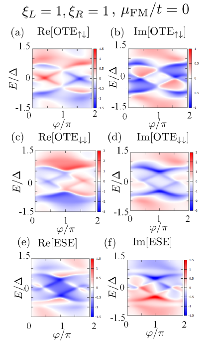
Figure 13: (a)-(d): The intensity plot of real part (a)((c)) and imaginary part (b)((d)) of odd-frequency spin-triplet even-parity (OTE) pair amplitude with $\downarrow\downarrow$ spin component $f_{odd}^{\downarrow,\downarrow}(E)$ and $\downarrow\downarrow$ spin component $f_{odd}^{\uparrow,\downarrow}(E)$. In (e) and (f), real part and imaginary part of even-frequency spin-singlet pair amplitude $f_{even}(E)$ is plotted.

IV Summary and Conclusions

In this paper, we have studied LDOS, current phase relation of Josephson current, energy levels of Andreev bound state and induced odd-frequency pairings in superconductor / ferromagnet / superconductor nanowire junction, where the magnetization penetrates into superconducting segment with a decay length $\xi$. We have chosen the chemical potential and SOC so that the topological superconducting regime hosting MF is realized for sufficiently large magnitude of $\xi$. We have found that when $\xi$ becomes larger, LDOS has a ZEP. On the other hand, if $\xi$ is shorter, zero energy state at the interface between superconductor and ferromagnet splits into two states. Accordingly, the behavior of Josephson current drastically changes. By tuning the parameters of the model, we have found an almost second-harmonic current-phase relation, $\sin 2\varphi$, with phase difference $\varphi$. Based on the analysis of ABS, we clarify that current-phase relation is determined by coupling of the states within the energy gap. We find that the emergence of crossing points of ABS is a key ingredient to generate $\sin 2\varphi$ dependence in current-phase relation. We further studied both the energy and $\varphi$ dependence of pair amplitudes in ferromagnet region. For long $\xi$, odd-frequency $s$-wave triplet component is dominant. The magnitude of the odd-frequency pair amplitude is enhanced at the energy level of ABS. On the other hand, when $\xi$ becomes shorter, not only odd-frequency pairing but also even-frequency pairing mixes.

Recently, $\sin 2\varphi$ behavior has been observed in S/F/S junctions, Pal et al. (2013) when ferromagnet is an insulator which has a spin filter effect. Thus to clarify the relevance of our obtained $\sin 2\varphi$ dependence to this experimental report is a challenging issue. In our paper, ballistic transport is assumed. If ferromagnet becomes diffusive, we can expect anomalous proximity effect Tanaka and Kashiwaya (2004); Tanaka et al. (2005a); Asano et al. (2006a); Tanaka et al. (2005b); Yokoyama et al. (2007, 2011) by odd-frequency spin-triplet $s$-wave pairing. Extension to this direction is also an interesting future study.

Appendix A Spatial profile of LDOS

In this appendix, we show spatial profile of LDOS of superconductor with decaying ferromagnetic order to understand “zero mode-non-zero mode crossover” more clearly. The ferromagnetic order decays from right to left similarly to Fig. 3(a). Since we will consider hybridization of two ZESs on the both edges of superconductor, we set the number of sites rather short, 200.

These profiles are shown in Fig. 14. For long enough decay length (Fig. 14(a)), ZEPs are localized on the both side of the nanowire, which is analogous to the situation where MFs are localized on the both edges of topological superconductor.Sticlet et al. (2012) If the decay length is decreased, however, the zero energy mode on the left comes close to the that on the right edge (Fig. 14(b)), then finally these two zero modes hybridize (Fig. 14(c)) to split into two (Fig. 14(d)).

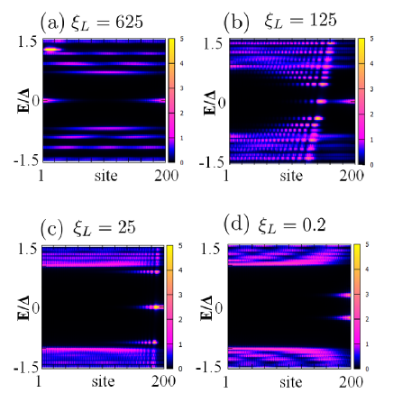
Figure 14: (a)-(d) The intensity plot of LDOS of the nanowire with decaying ferromagnetic order on top of the superconductor. The ferromagnetic order decays from right to left similarly to Fig. 3(a). Horizontal axis represents site index and vertical one does energy. Decay length of the ferromagnetic order is set as (a)$\xi_{L}=625$, (b)$\xi_{L}=125$, (c)$\xi_{L}=25$, and (d)$\xi_{L}=0.2$.

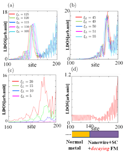
Figure 15: (a)-(c) The spatial dependence of LDOS at zero energy of the semiconducting nanowire with pair potential and decaying ferromagnetic order whose length is 200 sites. The several cases of LDOS are plotted for different decay length which is indicated by different colors as shown in each figure. (d) The spatial dependence of LDOS of the normal metal/nanowire junction system. The total length of this junction is set as 200 sites and the interface between normal metal and nanowire is located at site 140. In the nanowire segment, the pair potential and decaying ferromagnetic order with $\xi_{L}=125$ are also included similarly to (a)-(c). A schematic picture of this junction is shown below the plot.

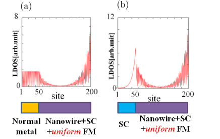
Figure 16: (a) The spatial dependence of LDOS of the normal metal/nanowire with pair potential and uniform ferromagnetic order junction system whose length is 200 sites. The interface is positioned at 50 sites. (b) The similar plot to (a) but the normal metal is replaced by $s$-wave superconductor. Schematic pictures of the junction are shown below each plot.

Below, we analyze the spatial profile of LDOS of the system we consider here in more detail especially focusing on at the zero energy. In Figs. 15(a)-(c), we plot this spatial dependence of LDOS for several cases of decay length. For large enough $\xi_{L}$ (Fig. 15(a) and (b)), we see the two ZEP: one is on the edge, $i.e.$ at 200 sites and another which is identified as broad peak is left from it (for Fig. 15(a), this ZEP is located at site $140\sim 150$ and for Fig. 15(b), it is at around site $180$). We notice that the position of the left peak is shifted if the decay length is changed and accordingly the behavior of the oscillations of LDOS left from the broad peak changes. However, we also find that the oscillations between the two peaks show the similar behavior. When the decay length is shorter than around $\xi_{L}=20$, the two peaks hybridize and are away from the zero energy (Fig. 15(c)). Further, we also calculate the spatial dependence of LDOS of normal metal/nanowire junction system with $\xi_{L}=125$. We set the interface at the site 140. The result is shown in Fig. 15(d). The board peak which is indicated in Fig. 15(a) spreads into the normal metal.

Actually, we can regard the two ZEPs explained above as the MFs. To make this statement more convincing, we calculate the spatial profile of the LDOS of the normal metal/nanowire with pair potential and uniform ferromagnetic order junction system as well as that of $s$-wave superconductor/nanowire junction system. These plots are shown in Figs. 16(a) and (b), respectively. The interface is located at site 50. In Fig. 15(a), the ZEP on the left which should be expected to appear at the interface penetrates into the normal metal segment. This is analogous to Fig. 15(d). Moreover, in Fig. 16(b), we can see the ZEP on the left (at site 50), however, as opposed to Figs. 16(a), this ZEP cannot spread into the left from the interface due to the superconducting energy gap. Therefore, ZEP cannot be stabilized and decays away from the interface. This behavior is similar to Figs. 15(a)(b), however, there is one difference: in Figs. 15(a)(b) due to the presence of non-uniform ferromagnetic order, there isn’t the explicit boundary which distinguishes the topologically trivial area and non-trivial one. Thus, the broad ZEP appears in Figs. 15(a)(b).

The comparison between the results of Fig. 15 and Fig. 16 implies that two ZEPs appeared in non-uniform case can be identified as two MFs.

References

- Golubov et al. (2004) A. A. Golubov, M. Y. Kupriyanov, and E. Ilichev, Rev. Mod. Phys. 76, 411 (2004).
- Buzdin (2005) A. I. Buzdin, Rev. Mod. Phys. 77, 935 (2005).
- Bergeret et al. (2005a) F. S. Bergeret, A. F. Volkov, and K. B. Efetov, Rev. Mod. Phys. 77, 1321 (2005a).
- Bulaevskii et al. (1977) L. N. Bulaevskii, V. V. Kuzii, and A. A. Sobyanin, JETP. Lett. 25, 291 (1977).
- Buzdin et al. (1982) A. I. Buzdin, L. N. Bulaevskii, and S. V. Panyukov, JETP Lett. 35, 179 (1982).
- Fulde and Ferrell (1977) P. Fulde and R. A. Ferrell, JETP. Lett. 25, 291 (1977).
- Larkin and Ovchinnikov (1965) A. I. Larkin and Y. N. Ovchinnikov, JETP 20, 762 (1965).
- Ryazanov et al. (2001) V. V. Ryazanov, V. A. Oboznov, A. Y. Rusanov, A. V. Veretennikov, A. A. Golubov, and J. Aarts, Phys. Rev. Lett. 86, 2427 (2001).
- Kontos et al. (2002) T. Kontos, M. Aprili, J. Lesueur, F. Genet, B. Stephanidis, and R. Boursie, Phys. Rev. Lett. 89, 137007 (2002).
- Robinson et al. (2006) J. W. A. Robinson, S. Piano, G. Burnell, C. Bell, and M. G. Blamire, Phys. Rev. Lett. 97, 177003 (2006).
- Tan (1997) Physica C 274, 357 (1997).
- Sellier et al. (2004) H. Sellier, C. Baraduc, F. m. c. Lefloch, and R. Calemczuk, Phys. Rev. Lett. 92, 257005 (2004).
- Robinson et al. (2007) J. W. A. Robinson, S. Piano, G. Burnell, C. Bell, and M. G. Blamire, Phys. Rev. B 76, 094522 (2007).
- Bergeret et al. (2001) F. S. Bergeret, A. F. Volkov, and K. B. Efetov, Phys. Rev. Lett. 86, 4096 (2001).
- Volkov et al. (2003) A. F. Volkov, F. S. Bergeret, and K. B. Efetov, Phys. Rev. Lett. 90, 117006 (2003).
- Eschrig (2011) M. Eschrig, Phys. Today 64, 43 (2011).
- Eschrig et al. (2003) M. Eschrig, J. Kopu, J. C. Cuevas, and G. Schön, Phys. Rev. Lett. 90, 137003 (2003).
- Keizer et al. (2006) R. S. Keizer, S. T. B. Goennenwein, T. M. Klapwijk, G. Miao, G.Xiao, and A. Gupta, Nature 439, 825 (2006).
- Sosnin et al. (2006) I. Sosnin, H. Cho, V. T. Petrashov, and A. F. Volkov, Phys. Rev. Lett. 96, 157002 (2006).
- Khaire et al. (2010) T. S. Khaire, M. A. Khasawneh, J. W. P. Pratt, and N. O. Birge, Phys. Rev. Lett. 104, 137002 (2010).
- Robinson et al. (2010) W. A. Robinson, J. D. S. Witt, and M. G. Blamire, Science 329, 59 (2010).
- Sprungmann et al. (2010) D. Sprungmann, K. Westerholt, H. Zabel, M. Weides, and H. Kohlstedt, Phys. Rev. B 82, 060505 (2010).
- Anwar et al. (2010) M. S. Anwar, F. Czeschka, M. Hesselberth, M. Porcu, and J. Aarts, Phys. Rev. B 82, 100501(R) (2010).
- Bergeret et al. (2004) F. S. Bergeret, A. F. Volkov, and K. B. Efetov, Phys. Rev. B 69, 174504 (2004).
- Bergeret et al. (2005b) F. S. Bergeret, A. L. Yeyati, and A. Martín-Rodero, Phys. Rev. B 72, 064524 (2005b).
- Linder et al. (2009) J. Linder, T. Yokoyama, and A. Sudbø, Phys. Rev. B 79, 054523 (2009).
- Xia et al. (2009) J. Xia, V. Shelukhin, M. Karpovski, A. Kapitulnik, and A. Palevski, Phys. Rev. Lett. 102, 087004 (2009).
- Lutchyn et al. (2010) R. M. Lutchyn, J. D. Sau, and S. Das Sarma, Phys. Rev. Lett. 105, 077001 (2010).
- Oreg et al. (2010) Y. Oreg, G. Refael, and F. von Oppen, Phys. Rev. Lett. 105, 177002 (2010).
- Sato and Fujimoto (2009) M. Sato and S. Fujimoto, Phys. Rev. B 79, 094504 (2009).
- Kitaev (2001) A. Y. Kitaev, Usp. Fiz. Nauk (Suppl.) 171, 131 (2001).
- Alicea (2012) J. Alicea, Rep. Prog. Phys. 75, 076501 (2012).
- Alicea et al. (2011) J. Alicea, Y. Oreg, G. Refael, F. von Oppen, and M. Fisher, Nature Communications 7, 412 (2011).
- Nayak et al. (2008) C. Nayak, S. H. Simon, A. Stern, M. Freedman, and S. Das Sarma, Rev. Mod. Phys. 80, 1083 (2008).
- Nadj-Perge et al. (2013) S. Nadj-Perge, I. K. Drozdov, B. A. Bernevig, and A. Yazdani, Phys. Rev. B 88, 020407 (2013).
- Nadj-Perge et al. (2014) S. Nadj-Perge, I. K. Drozdov, J. Li, H. Chen, S. Jeon, J. Seo, A. H. MacDonald, B. A. Bernevig, and A. Yazdani, 346, 602 (2014).
- Pöyhönen et al. (2014) K. Pöyhönen, A. Westström, J. Röntynen, and T. Ojanen, Phys. Rev. B 89, 115109 (2014).
- Pientka et al. (2014) F. Pientka, L. I. Glazman, and F. von Oppen, Phys. Rev. B 89, 180505 (2014).
- Braunecker and Simon (2013) B. Braunecker and P. Simon, Phys. Rev. Lett. 111, 147202 (2013).
- Klinovaja et al. (2013) J. Klinovaja, P. Stano, A. Yazdani, and D. Loss, Phys. Rev. Lett. 111, 186805 (2013).
- Pawlak et al. (2015) R. Pawlak, M. Kisiel, J. Klinovaja, T. Meier, S. Kawai, T. Glatzel, D. Loss, and E. Meyer, ArXiv e-prints (2015), eprint 1505.06078.
- Hoffman et al. (2015) S. Hoffman, J. Klinovaja, T. Meng, and D. Loss (2015), arXiv:1503.08762.
- Meng et al. (2015) T. Meng, J. Klinovaja, S. Hoffman, P. Simon, and D. Loss, Phys. Rev. B 92, 064503 (2015).
- Yu (1965) L. Yu, Act. Phys. Sin. 21, 75 (1965).
- H.Shiba (1968) H.Shiba, Prog.Theor.Phys. 40, 435 (1968).
- Rusinov (1969) A. Rusinov, Sov. Phys. JETP 29, 1101 (1969).
- Asano and Tanaka (2013) Y. Asano and Y. Tanaka, Phys. Rev. B 87, 104513 (2013).
- Tanaka and Kashiwaya (1997a) Y. Tanaka and S. Kashiwaya, Phys. Rev. B 56, 892 (1997a).
- Tanaka and Kashiwaya (1996a) Y. Tanaka and S. Kashiwaya, Phys. Rev. B. 53, 11957 (1996a).
- Kashiwaya and Tanaka (2000) S. Kashiwaya and Y. Tanaka, Rep. Prog. Phys. 63, 1641 (2000).
- Kwon et al. (2004a) H. Kwon, K. Sengupta, and V. Yakovenko, Eur. Phys. J. B 37, 349 (2004a).
- Asano et al. (2006a) Y. Asano, Y. Tanaka, and S. Kashiwaya, Phys. Rev. Lett. 96, 097007 (2006a).
- Law and Lee (2011) K. T. Law and P. A. Lee, Phys. Rev. B 84, 081304 (2011).
- Buchholtz and Zwicknagl (1981) L. J. Buchholtz and G. Zwicknagl, Phys. Rev. B 23, 5788 (1981).
- Hara and Nagai (1986) J. Hara and K. Nagai, Prog. Theor. Phys. 76, 1237 (1986).
- Hu (1994) C. R. Hu, Phys. Rev. Lett. 72, 1526 (1994).
- Tanaka and Kashiwaya (1995) Y. Tanaka and S. Kashiwaya, Phys. Rev. Lett. 74, 3451 (1995).
- Tanaka and Kashiwaya (1996b) Y. Tanaka and S. Kashiwaya, Phys. Rev. B. 53, 9371 (1996b).
- Beenakker (2013) C. W. J. Beenakker, Annu. Rev. Condens. Matter Phys. 4, 113 (2013).
- Yip (1993) S. Yip, J. Loe Temp. Phys. 91, 203 (1993).
- Tanaka and Kashiwaya (1997b) Y. Tanaka and S. Kashiwaya, Phys. Rev. B 56, 892 (1997b).
- Barash et al. (1996) Y. S. Barash, H. Burkhardt, and D. Rainer, Phys. Rev. Lett. 77, 4070 (1996).
- Kwon et al. (2004b) H.-J. Kwon, K. Sengupta, and V. Yakovenko, The European Physical Journal B - Condensed Matter and Complex Systems 37, 349 (2004b), ISSN 1434-6028.
- Berezinskii (1974) V. L. Berezinskii, JETP 20, 287 (1974).
- Black-Schaffer and Balatsky (2013) A. M. Black-Schaffer and A. V. Balatsky, Phys. Rev. B 87, 220506 (2013).
- Tanaka et al. (2007a) Y. Tanaka, A. A. Golubov, S. Kashiwaya, and M. Ueda, Phys. Rev. Lett. 99, 037005 (2007a).
- Tanaka et al. (2012) Y. Tanaka, M. Sato, and N. Nagaosa, J. Phys. Soc. Jpn. 81, 011013 (2012).
- Eschrig et al. (2007) M. Eschrig, T. Löfwander, T. Champel, J. Cuevas, and G. Schön, J. Low Temp. Phys. 147, 457 (2007).
- Asano et al. (2007a) Y. Asano, Y. Tanaka, and A. A. Golubov, Phys. Rev. Lett. 98, 107002 (2007a).
- Braude and Nazarov (2007) V. Braude and Y. V. Nazarov, Phys. Rev. Lett. 98, 077003 (2007).
- Asano et al. (2007b) Y. Asano, Y. Sawa, Y. Tanaka, and A. A. Golubov, Phys. Rev. B 76, 224525 (2007b).
- Eschrig and Löfwander (2008) M. Eschrig and T. Löfwander, Nature Physics 4, 138 (2008).
- Tanaka et al. (2007b) Y. Tanaka, Y. Tanuma, and A. A. Golubov, Phys. Rev. B 76, 054522 (2007b).
- Bakurskiy et al. (2014) S. V. Bakurskiy, A. A. Golubov, M. Y. Kupriyanov, K. Yada, and Y. Tanaka, Phys. Rev. B 90, 064513 (2014).
- Wakatsuki et al. (2014) R. Wakatsuki, M. Ezawa, Y. Tanaka, and N. Nagaosa, Phys. Rev. B 90, 014505 (2014).
- Ebisu et al. (2015) H. Ebisu, K. Yada, H. Kasai, and Y. Tanaka, Phys. Rev. B 91, 054518 (2015).
- Liu et al. (2015) X. Liu, J. D. Sau, and S. Das Sarma, Phys. Rev. B 92, 014513 (2015).
- Tanaka and Golubov (2007) Y. Tanaka and A. A. Golubov, Phys. Rev. Lett. 98, 037003 (2007).
- Pal et al. (2013) A. Pal, Z. Barber, and . M. B. J.W.A. Robinson, Nature Communications 5, 3340 (2013).
- Tanaka and Kashiwaya (2004) Y. Tanaka and S. Kashiwaya, Phys. Rev. B 70, 012507 (2004).
- Tanaka et al. (2005a) Y. Tanaka, S. Kashiwaya, and T. Yokoyama, Phys. Rev. B 71, 094513 (2005a).
- Asano et al. (2006b) Y. Asano, Y. Tanaka, and S. Kashiwaya, Phys. Rev. Lett. 96, 097007 (2006b).
- Tanaka et al. (2005b) Y. Tanaka, Y. Asano, A. Golubov, and S. Kashiwaya, Phys. Rev. B 72, 140503(R) (2005b).
- Yokoyama et al. (2007) T. Yokoyama, Y. Tanaka, and A. Golubov, Phys. Rev. B 75, 134510 (2007).
- Yokoyama et al. (2011) T. Yokoyama, Y. Tanaka, and N. Nagaosa, Phys. Rev. Lett. 106, 246601 (2011).
- Sticlet et al. (2012) D. Sticlet, C. Bena, and P. Simon, Phys. Rev. Lett. 108, 096802 (2012).