FUNDAMENTALS OF THE HOLOMORPHIC EMBEDDING LOAD-FLOW METHOD

Abstract

The Holomorphic Embedding Load-Flow Method (HELM) was recently introduced as a novel technique to constructively solve the power-flow equations in power grids, based on advanced complex analysis. In this paper, the theoretical foundations of the method are established in detail. Starting from a fundamental projective invariance of the power-flow equations, it is shown how to devise holomorphicity-preserving embeddings that ultimately allow regarding the power-flow problem as essentially a study in algebraic curves. Complementing this algebraic-geometric viewpoint, which lays the foundation of the method, it is shown how to apply standard analytic techniques (power series) for practical computation. Stahl’s theorem on the maximality of the analytic continuation provided by Padé approximants then ensures the completeness of the method. On the other hand, it is shown how to extend the method to accommodate smooth controls, such as the ubiquitous generator-controlled PV bus.

1 Introduction

The power grid has been hailed by the US National Academy of Engineering as the most influential engineering innovation of the 20th century [5]. Electrical power is what makes modern society tick, and the power grid has become a critical infrastructure. It is essentially a network of high voltage lines, transformers, and substations that carries bulk power over long distances, from power generation facilities to distribution substations.

The cornerstone problem of AC electrical power systems is the so-called power-flow study (also known as load-flow), which describes the steady state of the network under some given conditions. The problem can be written as follows, in terms of the current balance at each bus $i$:

$$\sum_{k}{Y_{ik}^{\text{(tr)}}V_{k}}+Y_{i}^{\text{(sh)}}V_{i}=\frac{S_{i}^{*}}{V_{i}^{*}}$$ (1)

where $Y_{ik}^{\text{(tr)}}$ are the elements of the transmission admittance matrix, $Y_{i}^{\text{(sh)}}$ are shunt admittances, and $S_{i}$ are constant-power injections going into the bus. The index $k$ runs over all buses including the swing bus, whose voltage $V^{\text{(sw)}}$ is specified as the reference. In its most basic form, the problem consists in solving (1) for the voltages $V_{i}$ (for all $i$ except the swing), for a given set of injections $S_{i}$. A variation of this problem, closer to actual practice, involves contemplating so-called PV buses, in which the voltage magnitude $|V_{i}|$ is kept constant by means of a variable injection of reactive power $Q_{i}$ by some generator (this amounts to adding new constraint equations and some corresponding new variables to (1), as it will be shown in § 5). In any case, note that the l.h.s. terms are all linear, but the constant-power injections appearing on the r.h.s. make the problem non-linear and multi-valued in general.

Many numerical methods have been devised for solving this problem since the beginning of computing. The earliest ones were based on Gauss-Seidel (GS) iteration [35], which has slow convergence rates but very small memory requirements. Most other methods are based on Newton–Raphson (NR) [32], which is generally better than GS because of its quadratic convergence properties.

Several improvements on the standard NR method were developed by exploiting the weak coupling between reactive power and voltage magnitude on the one hand, and real power and phase angles on the other, which yields good approximations in high-voltage transmission systems. Decoupling leads to smaller Jacobian matrices, which is a big computational gain in large networks, even when using sparse linear algebra techniques for maximum efficiency. Of all the various decoupled methods based on NR, the so-called Fast Decoupled Load Flow (FDLF) formulation of Stott and Alsac [29] has become the most successful and it is almost a de-facto standard in the industry, either in its original form or in one of its variants [34]. In addition to decoupling real and reactive power, the FDLF method factorizes the Jacobian matrix only once. Standard textbooks on power system analysis [10, 14, 6] describe all these methods in detail, and there exist widely available, open-source reference implementations of them, such as MATPOWER [38].

A common shortcoming of these traditional methods is their reliance on numerical iteration as the root-finding technique lying at the core of the procedure. As it is well-known, the success of NR or similar contraction-map iterations depends on the choice of an initial seed. Indeed, several authors have verified that since the powerflow problem is multi-valued, iterative methods not only exhibit this dependency, but may also behave erratically, since the different basins of attraction for the various solutions intertwine along fractal boundaries [31, 20, 12]. Certainly these problems may be overcome in the vast majority of cases if one devotes some time to explore different starting seeds and monitors the result to avoid undesired solutions. Additionally, many authors have developed additional techniques to improve the chance of convergence or even ensure global convergence properties [2, 13, 17], but their computational cost is significantly higher, their convergence is still not completely ensured in all cases, and human supervision is still needed to assess the different solutions obtained.

The Holomorphic Embedding Load-flow Method (HELM) method [33] was born out of the necessity to have a powerflow solution method that could run completely unattended and still produce reliable solutions. These characteristics are absolutely needed for building modern applications that perform massive searches in the state-space of the system, such as intelligent decision-support systems for grid operators. To give a simpler example, consider computing the solution of the system under the outage of one or more lines, which is a very common security assessment procedure. In that scenario NR-based methods have a non-negligible probability of failing, since the new solution may be “too far” from the previous undisturbed state.

From a numerical methods point of view, HELM is direct and constructive, and it does not require the choice of an initial seed. Based on a holomorphic embedding technique, it allows computing the formal power series corresponding to the desired solution in an unequivocal way. Then, thanks to a series of recent advances in the theory of Padé approximants, the numerical solution can be obtained with maximal guarantees (within the limits of floating point precision and round-off). The method thus obtains the desired solution if it exists, and conversely it unequivocally signals unfeasibility when such solution does not exist. It should be remarked that this method has been successfully implemented commercially, and proven able to solve networks of over 65,000 buses with performance that is competitive with traditional fast-decoupled methods.

A couple of clarifications regarding seemingly related methods is needed here. Although the idea of embedding is also used in so-called continuation powerflow methods [2], note that HELM is based on holomorphicity, which is a much more strict requirement than the simple smoothness properties required by homotopy. Moreover, as shown in this paper, the underlying formulation in terms of algebraic curves provides a global view that is harder to obtain otherwise. On the other hand, other authors have also explored the idea of exploiting the smoothness of the problem through the use of Taylor series expansions of the real and imaginary parts of the variables (or equivalently, their magnitudes and angles) [25, 36, 37]. This is of course very different from exploiting holomorphicity and analytic continuation.

In this paper, the theoretical foundations of the HELM method presented in [33] are established in detail. The emphasis is on algebraic curves, showing how two basic conceptual components of that field, namely polynomials and power series, apply to the powerflow problem. Additionally, it is shown how the method can accommodate the inclusion of any type of smooth control within exactly the same framework. The paper is structured as follows. Section 2 provides a quick overview of the method, summarizing the exposition given in [33] from a conceptual point of view. Section 3 discusses the foundations of the method by establishing the underlying mathematical structure of the theory, based on algebraic curves. This gives new insights into the powerflow problem. Section 4 provides the fundamentals for the more pragmatic aspect of the method, i.e. computing the solution through power series and analytical continuation. Then § 5 shows how the method can accomodate powerflow controls in a natural way. Some illustrative and pedagogical examples are fully worked out in the Appendix.

2 Overview of HELM

Our intention here is to show that the holomorphic embedding method is in fact a procedure to make the powerflow interpretable within the general framework of algebraic curves. This can be considered as looking at the problem from the viewpoint of polynomial systems. Doing this allows us to bring to the powerflow problem the amazing concepts of algebraic geometry, a subject that marries advanced complex analysis and abstract algebra, and dubbed by many authors as “the jewel” of XIX century mathematics. To do so, one needs to embed the complex voltage variables as holomorphic functions. For this it is necessary to avoid the use of $V_{i}^{*}(s)$, which is not holomorphic, and use instead the variable $\widehat{V}_{i}(s)$ as an independent holomorphic function. The original problem is recovered at the evaluation on the focal point by imposing the “reflection” condition $\widehat{V}_{i}(s)=V_{i}^{*}(s^{*})$.

Let us begin by reviewing the steps of the method in outline mode, and expand on their meaning later on. The first steps adopt the algebraic curve (polynomial) viewpoint, laying down the foundational concepts:

1. Embed the equations using a complex parameter $s$ as shown in [33]. To obtain holomorphicity in the next step, it is crucial that the variables $V_{i}^{*}$ are embedded as $V_{i}^{*}(s^{*})$, not as $V_{i}^{*}(s)$.

2. Use $\widehat{V}_{i}(s)$ instead of $V_{i}^{*}(s^{*})$; now the embedded equations define an algebraic curve and therefore the variables are holomorphic functions. However, once solved, we have to remember to request the reflection condition at $s=1$. Only such solutions represent physical (feasible) branches of the original powerflow problem; the rest are ghost solutions.

3. The system of equations are polynomial. Gröbner basis theory demonstrates that, using elimination techniques (for instance with lexicographical ordering), it is possible to arrive at a single polynomial equation in just one of the variables, say $V_{1}(s)$, while the rest, including of course $\widehat{V}_{k}(s)$, are recovered univocally in a triangular fashion. A single polynomial equation with $s$-dependent coefficients is by definition a plane algebraic curve.

4. Problems of existence of non ghost solutions (both operational and non-operational) can now be studied in terms of the topology, singularities, and branching points of the algebraic curve. For many small models, one may obtain illuminating results in closed form. This is not only useful for instructional analysis, but also for the exact study of small network equivalents, in particular the network algebraic equivalents that naturally arise in HELM, inspired in the theory of algebraic curves (these will be discussed in a forthcoming paper).

The rest of the steps deal with the computational aspects. The viewpoint thus switches from polynomials to power series that describe the local behaviour of algebraic curves at every point:

1. As the number of variables grow, it is not computationally feasible to use polynomial elimination techniques to solve for the algebraic curve explicitly. Instead, the method calculates the power series of the curve at the reference point $s=0$ (for a suitably chosen germ, which defines the branch), and then uses analytic continuation to try to reach the target point, $s=1$. The fact that one is dealing with an algebraic curve ensures that this series exists and has a non vanishing convergence radius.

2. The germ of choice at $s=0$ is the one that physically corresponds to an energized network with no constant-power loads or injections. It verifies the reflection condition.

3. The analytic continuation is computed by near-diagonal sequences of Padé approximants of the power series. Stahl’s theorem guarantees that the result is single-valued and maximal: if the approximants converge at $s=1$, we have obtained the solution; otherwise, there is no feasible powerflow.

Note that, under this procedure, the choice of a particular solution branch at $s=0$ uniquely determines the powerflow solution that is obtained at $s=1$, if it exists. The choice that the method proposes, which actually defines what we refer to as the operational solution, is easily identified as the state with zero constant-power load/generation and non-zero voltage throughout the network (i.e. zero power because the bus is open-circuited; note that zero power could also be achieved by short-circuiting, which gives rise to “dark” branches [33]).

This has been a summarized overview of the logic steps in building the theoretical scaffolding underlying the method. An actual numerical implementation would only deal with the calculation of power series and their Padé approximants [3], but such narrow mechanistic view of the method, although perfectly viable as a numeric procedure, would ignore the wealth of insights coming from the global aspects of the algebraic curve. We now leave the outline style and expand upon the motivation and foundations of each of these stages of the method.

3 Fundamentals I: the algebraic view

3.1 Preliminaries

The powerflow problem will be assumed to have the following general form:

$$\sum_{k}{Y_{ik}V_{k}}=\frac{S_{i}^{*}}{V_{i}^{*}}$$ (2)

where $Y_{ik}$ is the generalized admittance matrix containing the effects of all linear devices. This typically includes line admittances, transformers, (including phase-shifters), line susceptances, bus shunt admittances, constant-impedance loads, and constant-current injections, among others. The r.h.s. contains the constant-power injections, which are the nonlinear part.

Unless specified, indices run over all buses, including the swing bus which will be chosen at index $0$.

3.2 Motivation

The major motivation driving the methodology behind HELM originates in the projective invariance of equations (2), which strongly suggests how to study the system. If the voltages are rescaled by $V^{\prime}_{i}=\lambda V_{i}$, the resulting equations recover the same form, but with scaled injections:

$$\sum_{k}{Y_{ik}V^{\prime}_{k}}=|\lambda|^{2}\frac{S_{i}^{*}}{{V^{\prime}}_{i}^{*}}$$ (3)

As it is well-known in other areas of physics, this sort of invariance is something that deserves to be studied in its own right, as it often rewards us with insights and powerful results that would otherwise be lost (e.g., gauge theories in theoretical physics). In this case the projective invariance in (3) can be understood as a scale invariance linking the scales of voltages and power injections, so that the equations describe a whole family of powerflow problems at a time. Naturally, one fixes this invariance when choosing a particular reference value of the swing voltage, but the point here is that we would like to study this dependence. Therefore this leads one to consider an embedding technique by using $s=|\lambda|^{2}$ as a new variable of the problem. The family corresponds to all real and positive values of $s$.

However, there are strong reasons to work with a complex embedding parameter. The first reason is that equations (2) are algebraic, and therefore they can always be reduced to polynomials by means of elimination techniques, as shown in § 3.5. Therefore it makes sense to work in the complex domain, where the fundamental theorem of algebra guarantees that all zeros exist. Another reason is that, using a suitable form of the embedding as shown below, the problem is converted into an algebraic curve. This opens up a plethora of techniques and results from complex analysis. Most of them derive from holomorphicity, i.e. complex analyticity of the voltages with respect to the complex embedding parameter. Therefore there is nothing to lose and a lot to win by working in the complex $s$-plane (eventually, the functions are evaluated at the focal real value of $s$ to get the desired voltages). In fact the main proposition in HELM is to look at the powerflow as a particular problem within the theory of algebraic curves. This requires considering complex variables and holomorphic functions.

3.3 Complex embedding

The proposed embedding consists in introducing a complex parameter $s$ into (2). A natural possibility, which will be referred to as the minimal embedding, is the one suggested by the projective invariance discussed above:

$$\sum_{k}{Y_{ik}V_{k}(s)}=s\frac{S_{i}^{*}}{V_{i}^{*}(s^{*})}$$ (4)

Note how one recovers exactly the powerflow equations of (3) for real, positive values of $s$. On the other hand, it is key that the voltage parameters $V_{i}^{*}$ are embedded as $V_{i}^{*}(s^{*})$, not as $V_{i}^{*}(s)$, since the former verifies the Cauchy-Riemann equations and the latter does not. The idea is also inspired by Schwarz reflection principle [16], and its use will become clear in the next section.

3.4 Holomorphicity and the reflection condition on $V,\widehat{V}$

Since complex conjugation does not preserve holomorphicity, the embedded system (4) must be formally doubled with its mirror image:

$$\begin{split}\sum_{k}{Y_{ik}V_{k}(s)}&=s\frac{S_{i}^{*}}{\widehat{V}_{i}(s)}\\ \sum_{k}{Y_{ik}^{*}\widehat{V}_{k}(s)}&=s\frac{S_{i}}{V_{i}(s)}\end{split}$$ (5)

where $V_{i}(s),\widehat{V}_{i}(s)$ must be considered as two sets of independent holomorphic functions. Note that here the hat denotes just a different symbol, not complex conjugation. Once the solution for both sets is found, if the following equality holds

$$\widehat{V}_{i}(s)=V_{i}^{*}(s^{*}),$$ (6)

which will be referred to as the reflection condition, then the two sets of equations in (5) are just complex conjugates of each other, and the embedded system (4) is recovered. Note however that the doubled system (5) may contain solutions that do not satisfy the reflection condition (6) when evaluated at $s=1$ and therefore are not physical solutions to the original powerflow problem (these will be referred to as ghost solutions). Therefore the method consists in solving the algebraic system (5) and requiring the additional condition (6) to hold at $s=1$. Then, among the non-ghost solutions, if any, one will identify the one representing the normal operational condition as a well-defined specific branch of the algebraic curve (white branch). All other non-ghost solutions are black branches, i.e. physical in principle but representing low-voltage, non-operational scenarios. If all the algebraic solutions are ghost, the original parametric powerflow problem has no solution.

3.5 Elimination polynomial

Eliminating denominators, the system (5) becomes a set of polynomial equations in several variables. There exist many elimination techniques to solve these [30], such as classical resultants, characteristic sets, and Gröbner bases. Although in practice the HELM method does not use any of these computer algebra methods, Buchberger’s algorithm on Gröbner basis theory [4] may be invoked to prove that it is always possible to carry out a complete elimination procedure, arriving at a polynomial equation in only one of the variables (say, $V_{1}$):

$$\mathfrak{P}(s,V_{1})=\sum_{n=0}^{\deg\mathfrak{P}}{a_{n}(s)V_{1}^{n}}=0$$ (7)

Furthermore, using lexicographical monomial ordering, the elimination is triangular: all the other variables $\widehat{V}_{1},V_{2},\widehat{V}_{2},V_{3}$, etc., are expressed explicitly as polynomials in the previous ones. Given a solution $V_{1}(s)$ to (7), all other values $V_{i}(s),\widehat{V}_{i}(s)$ are then obtained by simple progressive back-substitution.

The degree $\deg\mathfrak{P}$ of this polynomial is in general rather large (of order exponential in the number of buses), but the key points here are that the degree is always finite and the coefficients $a_{n}(s)$ are polynomial in $s$. This means that (7) is a plane algebraic curve. Thus the powerflow problem has been converted, via the embedding procedure, into the study of algebraic curves on the complex plane, which is a field in which there is a plethora of results to exploit and build upon [9, 15]. Algebraic curves are essentially linked to Riemann surfaces [26, 7], another field rich in powerful results.

3.6 Algebraic curves. Branches

One of the most immediate results that can be reaped concerns the analysis and interpretation of the multiple solutions of the powerflow problem, and the collisions among them, in particular at voltage collapse points. Now all possible powerflow solutions are characterized as branches of the corresponding algebraic curve defined by (7). Branch collisions take place at the so-called branch points of the curve, which are the values of $s$ for which a zero of $\mathfrak{P}(V_{1})$ has multiplicity 2 or greater. This, together with the reflection condition (6), allows us to interpret feasibility and voltage collapse in the powerflow problem under a new light. Algebraic curves provide a global view with far greater analytical power than numerical techniques such as Newton–Raphson, which only exploit local properties. For instance, a traditional continuation powerflow [2] can calculate and analyze the collapse point in terms of a saddle-node bifurcation, but the theory presented here reveals it more specifically as two branches of a (complex) algebraic curve merging at a branch point.

At each particular point $s$ of the complex plane, the branches can be categorized into these groups:

• Ghost branches: these correspond to solutions that fail to satisfy the reflection condition. Therefore, when $s$ is real positive, they are not physical powerflow solutions.

• Feasible branches: these satisfy the reflection condition and therefore represent physically possible powerflows when $s$ is real positive. However, only one of these corresponds to the normal operating state of a power network, as it will be shown below.

Voltage collapse is therefore understood as a collision in the $s$-plane of the operational branch with another one and the emergence of a couple of ghost branches as a result.

Algebraic techniques allow the calculation of all branches simply as the roots of polynomial $\mathfrak{P}(s,V_{1})$. Calculation of all branch points is also accomplished by well-known techniques, such as the calculation of the discriminant of $\mathfrak{P}(s,V_{1})$ (the resultant of the two polynomials $\mathfrak{P},\partial\mathfrak{P}/\partial V_{1}$). Appendix A demonstrates the power of this analysis in an example where the curve and its branch points can be explicitly calculated. However, since the degree of the algebraic curve grows exponentially with the number of buses, such explicit calculations can only be carried out for very small networks. Several authors [19, 18, 11, 22, 21] have explored these computer algebra techniques for simultaneously obtaining all solutions to the powerflow problem (although not in an embedded setting), and the typical size that is computationally feasible remains at around four to five buses maximum. Therefore the exposition turns now to the method for computing solutions for networks of any size.

4 Fundamentals II: the analytical view

4.1 Power series

As it is customary in the field of algebraic curves, for practical computations one uses the power series representation developed about some reference point. Since the $V_{i}(s)$ are holomorphic, their power series contain all the information needed to reconstruct the functions in their full domain of holomorphy (which in this case, being algebraic curves, is the full complex plane except a finite number of singular points), beyond the convergence radius of the series. Each power series defines a different branch and in this sense, they are referred to as “germs” of the branches of the algebraic curve [1]. This full reconstruction is provided by the powerful Weierstrass analytic continuation procedure, and it is what allows HELM to extend the germs from local to global branches.

In sum, working with power series allows practical computation in networks of any size, and holomorphicity ensures that, at least in principle, calculations at points far away from the reference can be carried out through analytic continuation.

4.2 The choice of branch. Operational solution

The next problem consists in selecting the proper branch. Since the goal is to obtain the operational solution of the original powerflow (2), some criterion is needed to select a branch out of the multiple ones in system (5). Drawing from the physics behind the problem, it can be argued that $s=0$ provides the privileged reference point for an unambiguous choice. At $s=0$ the system represents a power network in which the constant-power injections (whether load or generation) are zero. At each bus, this situation can be achieved either by open-circuit, in which case the voltage is non-zero, or by short-circuit, in which case the voltage is zero and the right-hand side $sS_{i}^{*}/\widehat{V}_{i}(s)$ in (5) approaches the value of the bus fault current. Requiring that $V_{i}(0)\neq 0$ throughout, i.e. open circuiting all buses except the swing, provides a unique answer, which will be referred to as the white branch (at $s=0$).

Reference [33] shows in detail the mechanics to compute the power series terms of this white germ, up to any desired order, through a constructive procedure involving the repeated solution of a linear system in sequence. One important point is that this procedure automatically enforces the reflection condition; the white germ clearly satisfies this condition at $s=0$. Regarding a power series as the identity mark of a branch, and Weierstrass analytic continuation as a propagation of this identity to other parts of the $s$-plane, HELM postulates that the operational solution sought at $s=1$ must have the same identity and therefore is the analytic continuation of the white germ.

4.3 Analytic continuation and single-valuedness

In HELM one assumes that the powerflow problem corresponds to the operational state of some real network. Therefore, regardless of the particular method used to perform the analytic continuation of the white germ discussed above, we need to enforce the single-valuedness of the procedure in order to obtain a single solution. It is well-known that analytic continuation of a holomorphic function from a given point $s_{a}$ to a point $s_{b}$ along different paths may yield different values of the function at $s_{b}$ just by following different paths. This reflects the fact that the algebraic curve is actually one whole multi-valued holomorphic function, not simply a collection of disjoint branches. This “branch identity loss” can only happen if both paths enclose a singular point (branching point).

The way to solve this issue is standard in complex analysis. One must remove from the complex plane (technically, from the extended complex plane $\mathbb{C}_{\infty}$, the Riemann sphere) a connected set of lines $\Gamma$ (branch cuts) connecting all branch points. Then the complement $\mathbb{C}_{\infty}\setminus\Gamma$ will be simply connected (no holes) and the analytic continuation along any path on the remaining plane will be guaranteed to provide a unique result, since it is no longer possible to have paths encircling a branch point (because they would have to cross one of the removed lines). This is for instance what is done in the definition of some elementary multi-valued complex functions, such as the square root, in which the choice of the branch cut along $(-\infty,0)$ fixes the conventional meaning of the principal value of the square root (i.e. the meaning of the symbol $\sqrt{z}$).

Note that the choice of branch cuts is a priori arbitrary (as long as they connect all branch points), but every choice leads in principle to a different single-valued function. Therefore the problem is not only achieving single-valuedness, but also choosing the set $\Gamma$ (branch cuts) in such a way that the analytical continuation of the white germ at $s=1$ gives a solution that makes physical sense. Our argument, based on physical plausibility, is that the operational solution to the powerflow problem exists if and only if, using the complex embedding (4), the white germ is analytic-continuable along all values $0<s\leq 1$ on the real axis. Therefore the only a priori requirement on the choice of branch cuts is that they do not contain any part of this particular continuation path. Intuitively, one requires that the whole family of projectively equivalent powerflow problems up to $s=1$ retains the same identity as the germ at $s=0$.

4.4 Maximality of the analytic continuation: Stahl’s Theorem

A key fact is that there is a very natural way to choose the branch cuts. Since the problem is described by an algebraic curve, $V_{i}(s)$ is holomorphic with a finite number of branch points. In this case, Stahl’s theorem [27, 28], which proves an earlier conjecture by Nuttall [23], states the following:

1. There exists a unique extremal domain $D$ in which the function has a single-valued analytic continuation. In other words, there exists a choice of branch cuts $\Gamma$ enforcing single-valuedness such that the resulting domain (in our case $\mathbb{C}_{\infty}\setminus\Gamma$) is the “biggest” one possible (the precise mathematical measure for this is the concept of logarithmic capacity; this result asserts that there exists a unique choice of cuts $\Gamma$ that has minimal logarithmic capacity).

2. The sequence $[L_{j}/M_{j}]$ of Padé approximants converges in capacity to the function in the extremal domain $D$ for any sequence of indices satisfying $L_{j}+M_{j}\rightarrow\infty$ and $L_{j}/M_{j}\rightarrow 1$ as $j\rightarrow\infty$.

In other words, the near-diagonal Padé approximants of the white germ converge to the single-valued function in its maximal domain of analytic continuation, which in this case is everywhere on the $s$-plane except on the set of branch cuts $\Gamma$. This last step therefore rounds up the method, providing both a practical way to calculate the analytical continuation and an unequivocal test for the existence of the operational solution.

Fig. 1 shows a schematic view of a minimal cut set $\Gamma$. The set has minimal logarithmic capacity in the complex $u$-plane, where $u=1/s$. For the two-bus problem, the system has only two branch points and therefore in that case $\Gamma$ is simply a straight segment joining them (see the Appendix). In the general case, $\Gamma$ would be more complicated. If one were interested in calculating $\Gamma$, it is interesting to note that the zeros and poles of the Padé approximants mentioned above tend to accumulate on this set. In any case, from the point of view of the powerflow problem, and in particular the existence of an operational solution, the key question is whether or not the set $\Gamma$ obstructs the path along the real axis from $s=0$ to $s=1$ (in the $u$-plane, from $u=+\infty$ to $u=1$).

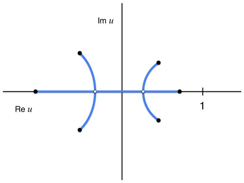
Fig. 1: Schematic example of the minimal cut set $\Gamma$ in the complex $u$-plane, for an algebraic curve with six branch points (black dots). The diamond-shaped points are auxiliary connecting points. In this example, the powerflow problem has an operational solution, since the path from $u=+\infty$ (i.e. $s=0$) along the real axis can reach $u=1$ without encountering the cut set, which means that the white germ has an analytic continuation along that path. Stahl’s theorem proves that the analytic continuation can be provided by Padé approximants.

One subtle point remains: could it ever happen that the excluded set $\Gamma$, in spite of being of minimal size, crosses or covers the interval $0<s\leq 1$ when there is otherwise no obstruction to the analytic continuation along that specific path corresponding to the projective family? After all, Stahl guarantees that Padé approximants converge in a maximal domain, but says nothing about this specific path. The answer lies in the choice of embedding, as covered in the following section.

Note that the reverse condition is adequately covered: if the operational powerflow solution does not exist, the procedure will detect so. By our definition above, if the solution does not exist it means that the white germ is not analytic-continuable along all values $0<s\leq 1$ on the real axis, which is something that can be easily tested by checking the convergence of the Padé approximants.

4.5 Choice of embedding

Looking back at (4), it should be remarked that it is certainly not the only possible embedding satisfying the requirements of the method. For instance, one could also embed all shunt elements:

$$\sum_{k}{Y_{ik}^{\text{(tr)}}V_{k}(s)}=-sY_{i}^{\text{(sh)}}V_{i}(s)+s\frac{S_{i}^{*}}{V_{i}^{*}(s^{*})}$$ (8)

Here $Y_{ik}^{\text{(tr)}}$ represents the transmission admittances, which satisfy $\sum_{k}{Y_{ik}^{\text{(tr)}}}=0$ for all $i$ (the indices include the swing bus); while $Y_{i}^{\text{(sh)}}$ represent shunt terms, either from load models or from lines and transformers. The reference state $s=0$ in this case can be physically interpreted as the line charging susceptances being completely compensated, waiting for the loads to be connected. This embedding would yield at $s=0$ a reference solution having all voltages equal to the swing bus. The authors have used this type of embedding for years and think that it is probably the most reasonable identity to assign to the empty network. It will be denoted as HELM’s canonical embedding.

Another example would be to additionally embed the resistive parts of $Y^{\text{(tr)}}$:

$$j\sum_{k}{B_{ik}^{\text{(tr)}}V_{k}}=-s\sum_{k}{G_{ik}^{\text{(tr)}}V_{k}}-sY_{i}^{\text{(sh)}}V_{i}+s\frac{S_{i}^{*}}{\widehat{V}_{i}}$$ (9)

so that the resulting linear systems for computing the white germ only involve the real matrix $B_{ik}^{\text{(tr)}}$, which could be considered as numerically more efficient. Yet a further example would be to extend the embedding to the non-symmetric elements of $B_{ik}^{\text{(tr)}}$ (those originating from phase-shifting transformers), so that the final matrix is symmetric and therefore more efficient to factorize via Cholesky instead of a general LU decomposition.

However, the choice of embedding is not completely harmless. Different forms of the embedding result in different algebraic curves, having different branching points. It can be shown that the introduction of additional embedded terms in (4), as suggested above, normally results in additional branch points in the resulting curve. Vast numerical evidence shows that these additional singularities are harmless in the case of (8), since the corresponding Stahl cuts still do not cover the interval $0<s\leq 1$ and then the numerical solution is exactly the same. But in other embeddings, the result may be that, for powerflow cases where the operational solution at $s=1$ does exist, the additional branching points could introduce obstacles to the convergence of the Padé approximants, by way of the minimal set $\Gamma$ covering the point $s=1$. This is a rather academic problem, since in practice one needs to use artificial embeddings in order to find a single example of this phenomenon. It is however an interesting question to find a general way to characterize the relationship between the functional form of the embedding and the resulting minimal set $\Gamma$, in order to prevent the use of such problematic embeddings. This problem is yet unexplored, but it is linked to the Pólya-Chebotarev problem, a current research topic in advanced complex analysis [8, 24]. Nonetheless the authors will report some considerations about this problem in a forthcoming paper.

For the two-bus case, it can be shown rigorously that the minimal embedding (4) is free of this problem (see Appendix A). For the general $n$-bus case, there is extensive numerical evidence as well as strong heuristic reasons to support this as well. The most important one is that the minimal embedding matches the physically realizable picture of an energized network in which the injections are progressively turned on, starting from the no-load state. Evidence shows that the canonical embedding (8) is also free of problems; in fact it could be argued that the physical picture is even more natural in this case.

This concludes the foundations for the completeness of the method:

• If the operational solution exists, the method will find it: Stahl’s theorem and the choice of the canonical embedding ensure that the Padé approximants converge (in capacity measure) to the solution.

• If the operational solution does not exist, the method will detect so: non-convergence of the Padé approximants (along the path $0<s\leq 1$ on the real axis) necessarily implies an unfeasible powerflow, because if they did converge they would be the analytical continuation of the white germ and therefore the powerflow solution, thus contradicting the assumption.

5 Extensions: the role of controls as constraints

In the context of the powerflow problem, controls are seen as additional mathematical constraints on the voltages or on some other magnitude (which can always be expressed ultimately in terms of the voltages). Primary examples are voltage regulation at generator buses, which gives rise to the so-called PV buses, or on-load tap changing (OLTC) transformers, or switched capacitor/reactor banks (shunts). Since the powerflow is only concerned with the steady state, any dynamical aspects are ignored, and thus only the the stable final state of controls is considered. For instance, in a PV regulated bus it is only needed to consider the voltage modulus setpoint, and the mathematical constraint would be simply $V_{k}V_{k}^{*}=|V_{k}^{\text{sp}}|^{2}$. Obviously, for each new constraint equation added to the system one needs to free some other parameter in the equation, to balance the degrees of freedom. In the PV example, one normally designates the local reactive injection $Q_{k}$ as the new control variable. In the case of a remote voltage-controlled PQ bus $k$, the new variable could be some other $Q_{k^{\prime}}$ or some weighted combination of reactive injections.

The HELM method can seamlessly incorporate any type of control, as long as the associated constraints can be expressed as some algebraic function of the voltages or flows. This is always the case since all controls can be expressed as a polynomial equation in the steady state. These will be referred to as algebraic controls. This way the system is still described by an algebraic curve and thus all the fundamental properties of the method are preserved. In practice this means that all “smooth” controls can be accommodated in HELM, but there are two characteristics that break holomorphicity and therefore need to be treated outside of HELM methodology: saturation limits and discreteness. Real controls always exhibit resource limits, and sometimes also discreteness effects. The most prominent examples of saturation limits are the $(Q_{\text{min}},Q_{\text{max}})$ capability limits in generator buses and the tap ratio range limits in OLTC transformers. The latter are also prime examples of discreteness (tap ratio steps) and threshold activation effects (control deadband). All of these issues can be dealt with via successive application of the algebraic method, combined with discretization techniques such as relaxation and/or combinatorial search. Further details and a complete framework for dealing with limits and discreteness will be the subject of a forthcoming publication. The exposition here will only deal with algebraic controls, focusing on the HELM fundamentals.

5.1 Algebraic controls

The introduction of controls in the HELM framework is guided by the fundamentals exposed in the previous section. It basically amounts to an adequate embedding of the constraint expression, in a way that preserves the algebraic nature of the problem (and therefore holomorphicity) and also attains a reference solution at $s=0$ that makes physical sense as an energized, no load network. On the other hand, for the addition of each new constraint one has to designate one new free variable, in order to keep the number of equations and unknowns balanced. This is best exemplified by showing how this can be done in the simplest and most ubiquitous case, the PV node.

Let us consider the general powerflow equations of a network as in (2), except that now the buses are labeled into two sets: the $\{PV\}$ set, having $n_{\text{PV}}$ buses, and the $\{PQ\}$ set having $n_{\text{PQ}}$. There are $n_{\text{PV}}$ new constraints $V_{k}V_{k}^{*}=|V_{k}^{\text{(sp)}}|^{2}$, which are clearly algebraic. In a PV bus, voltage control is achieved by regulating the injection of reactive power local to the bus. This naturally suggests the new variables of the system, needed to counterbalance the constraints.

These constraints need to be holomorphically embedded using the simplest functional form possible in order to avoid introducing extra singularities in the $s$-plane. In this case one cannot simply use a constant function $V_{k}(s)V_{k}^{*}(s^{*})=|V_{k}^{\text{(sp)}}|^{2}$, since the voltages at $s=0$ could not satisfy it without some reactive injection, and these are switched off at the reference state. The simplest valid form is a linear function interpolating between the natural values of voltage at $s=0$ and the desired setpoint at $s=1$. Assuming without loss of generality that the swing has a unit voltage setting, the embedding is simply:

$$V_{k}(s)V_{k}^{*}(s^{*})=1+s\left(|V_{k}^{\text{(sp)}}|^{2}-1\right)$$ (10)

Separating nodes into the PQ set and the PV set, this is the proposed canonical embedding:

$$\begin{split}\sum_{l}Y_{kl}^{\text{(tr)}}V_{l}(s)&=-sY_{k}^{\text{(sh)}}V_{k}(s)+s\frac{P_{k}}{V^{*}_{k}(s^{*})}-j\frac{Q_{k}(s)}{V^{*}_{k}(s^{*})}\\ \sum_{j}Y_{ij}^{\text{(tr)}}V_{j}(s)&=-sY_{i}^{\text{(sh)}}V_{i}(s)+s\frac{S^{*}_{i}}{V^{*}_{i}(s^{*})}\end{split}$$ (11)

where the indices $k\in\{PV\}$ and $i\in\{PQ\}$, and the rest go over all buses unless otherwise noted. The enlarged system (10)+(11) preserves all algebraic properties of the original, so that all of HELM theory and methods apply. The variables $\widehat{V}_{i}$ would be introduced analogously, and the new system would then consist of $3n_{PV}+2n_{PQ}$ equations: $2(n_{PV}+n_{PQ})$ equations coming from (11) and its reflection, plus $n_{PV}$ new equations coming from (10), whose reflection yields identically the same expression. Correspondingly, there are $3n_{PV}+2n_{PQ}$ variables: $2(n_{PV}+n_{PQ})$ variables $Vi,\widehat{V}_{i}$, plus $n_{PV}$ new variables $Q_{k}$.

Moreover this embedding allows a meaningful reference state at $s=0$, namely, the zero injection state. Note that this requires that the new variables $Q_{k}(s)$ be zero at $s=0$. The voltages then become all equal to the swing bus voltage at $s=0$.

The numerical procedure described in [33] would then be applied analogously. Using the power series expansion for the variables $V(s)=\sum_{N}V[N]s^{N}$ and $Q(s)=\sum_{N}Q[N]s^{N}$, and substituting into equations (10)+(11), one would obtain a linear system where the coefficient matrix is fixed, and the terms at order $N$ can be obtained from the results computed at the preceding orders. Solving this system sequentially in successive orders and computing the Padé approximants as shown in [33] would conclude the method.

However, the fact that the system is converted in this fashion into a sequence of linear systems provides the chance to perform some powerful simplifications, simply following standard transformations akin to Gaussian elimination. For instance, in this case it can be shown that the linear system can be reduced from dimension $3n_{PV}+2n_{PQ}$ to $n_{PV}+2n_{PQ}$. Further details on the computationally efficient implementation of this control and several others will be the subject of a future publication.

This concludes the method for incorporating PV nodes. It should be remarked that other types of controls, even sophisticated ones involving several control variables and controlled magnitudes (e.g., area interexchange schedules) can be integrated in HELM analogously in an exact way.

6 Conclusion

The HELM method and its associated theory opens up new perspectives on the powerflow problem. It sheds new light on the problems of existence, multiplicity of solutions, and voltage collapse. It achieves this through the use of advanced concepts in algebraic geometry and complex analysis. Through the study of a fundamental projective invariance, it is shown how the original problem transforms into the study of an algebraic curve. Then recent advances in the field of rational approximants provide a practical way to compute solutions through power series expansions, and additionally confer completeness to the method by virtue of a theorem on the maximality of the analytic continuation provided by the Padé approximants.

Appendix A Full HELM-based solution of the two-bus problem

The two-bus model provides an easy and rather complete showcase for all the elements of HELM theory. It allows exemplifying all the fundamentals exposed in the preceding sections through explicit, closed form calculations. Let us start with the powerflow equations written in dimensionless magnitudes $U\equiv\frac{V}{V_{0}}$ and $\sigma\equiv\frac{ZS^{*}}{|V_{0}|^{2}}$:

$$U=1+\frac{\sigma}{U^{*}}$$ (12)

Solving separately for the real and imaginary parts of $U$, it is straightforward to arrive at the exact solution:

$$U=\frac{1}{2}\pm\sqrt{\frac{1}{4}+\sigma_{R}-\sigma_{I}^{2}}+j\sigma_{I}$$ (13)

subject to the condition $\Delta\equiv\frac{1}{4}+\sigma_{R}-\sigma_{I}^{2}\geq 0$, where $\sigma_{R},\sigma_{I}$ are the real and imaginary parts of $\sigma$, respectively. It is important to realize that if this condition is not met, then there is no solution to the powerflow problem. Therefore as a parametric ordinary equation the system has the two solutions (13) if $\Delta\geq 0$, and none if $\Delta<0$.

Now consider the corresponding embedded system, written in explicit polynomial form:

$$\begin{split}U(s)\widehat{U}(s)-\widehat{U}(s)-s\sigma&=0\\ \widehat{U}(s)U(s)-U(s)-s\sigma^{*}&=0\end{split}$$ (14)

In this case it is straightforward to carry out the elimination procedure by hand. Eliminating $\widehat{U}$ from the second equation and substituting in the first, one readily arrives to the algebraic curve:

$$\mathfrak{P}(s,U)=U^{2}-(1+2js\sigma_{I})\,U-s\sigma^{*}=0$$ (15)

and the other variable can be obtained in terms of $U$, also in polynomial form, by eliminating $U\widehat{U}$ from (14):

$$\widehat{U}=U-2js\sigma_{I}$$

Solving (15) one readily obtains the two branches of this curve, together with the corresponding ones for $\widehat{U}(s)$:

$$\begin{split}U(s)_{\pm}&=\frac{1}{2}\pm\sqrt{\frac{1}{4}+s\sigma_{R}-s^{2}\sigma_{I}^{2}}+js\sigma_{I}\\ \widehat{U}(s)_{\pm}&=\frac{1}{2}\pm\sqrt{\frac{1}{4}+s\sigma_{R}-s^{2}\sigma_{I}^{2}}-js\sigma_{I}\end{split}$$ (16)

The branches exist everywhere on the complex $s$-plane (and coincide at the two branch points). However, for them to be a solution of the powerflow problem, the reflection condition $\widehat{U}(s)=U^{*}(s^{*})$ has to be satisfied at $s=1$. Additionally, the branch containing the operational solution, if it exists, is easily identified as the one with the plus sign in (16).

One verifies that the reflection condition is satisfied everywhere on the $s$-plane except at the points where the discriminant $\Delta(s)\equiv\frac{1}{4}+s\sigma_{R}-s^{2}\sigma_{I}^{2}$ becomes real negative (in this case, this holds for both branches). Solving for the roots of this discriminant,

$$s_{\pm}=\frac{\sigma_{R}\pm|\sigma|}{2\sigma_{I}^{2}}$$ (17)

we find that the reflection condition fails for values $s<s_{\text{-}}$ and $s>s_{\text{+}}$ on the real axis. Note that the points $s_{\pm}$ in (17) are the branch points of the algebraic curves (16), i.e. the points where the $(+)$ and $(-)$ branches collide. The value $s_{\text{-}}$ is always negative; since we are interested in reaching $s=1$, the condition for existence of powerflow solutions is therefore $s_{\text{+}}\geq 1$. From (17) above, this translates to $\frac{1}{4}+\sigma_{R}-\sigma_{I}^{2}\geq 0$, thus recovering the condition found in (13).

On the other hand, these intervals $s<s_{\text{-}}$ and $s>s_{\text{+}}$ form a simply connected set of branch cuts of the algebraic curve, as they join the two branch points through infinity (or equivalently, through $0$ in the $1/s$-plane). Since the arc of minimal logarithmic capacity joining two points is always a straight segment, this proves that this is the minimal cut-set in the sense of Stahl. Therefore the Padé approximants, for both germs, will fail to converge for $s<s_{\text{-}}$ and $s>s_{\text{+}}$ on the real axis. This confirms the general theory: the sequence of near-diagonal Padé approximants converge to the solution when it exists, and they do not converge when it does not.

A.1 The PV case

The two-bus PV case solves analogously, with the addition of an embedded constraint as in (10) and the corresponding new variable $Q$. It is also straightforward to carry out the elimination procedure by hand, but it is interesting to see how Buchberger’s algorithm [4] would do it. Writing the constraint as $K(s)\equiv 1+s(|V^{\text{sp}}|^{2}-1)$, and choosing lexicographic order $U\prec Q\prec\widehat{U}$, the system is now written as the following polynomial ideal in the ring of polynomials of three variables:

$$\left<\widehat{U}U-\widehat{U}+jszQ-szP,\quad\widehat{U}U-jsz^{*}Q-U-sz^{*}P,\quad\widehat{U}U-K(s)\right>$$

where we have defined $z\equiv\frac{Z}{|V_{0}|^{2}}\equiv r+jx$. The Gröbner elimination procedure is simplified in this case if one assumes a lossless line, $r=0$:

$$\left<\widehat{U}U-\widehat{U}-sxQ-jsxP,\quad\widehat{U}U-sxQ-U+jsxP,\quad\widehat{U}U-K(s)\right>$$

Elimination of the leading monomial $\widehat{U}U$ by subtracting the first two polynomials, plus using the third one, leads to:

$$\left<\widehat{U}U-K(s),\quad\widehat{U}-U+2jsxP,\quad sxQ+U-jsxP-K(s)\right>$$

To eliminate the leading monomial, multiply the second polynomial by $U$ and subtract. This yields the Gröbner basis in triangular form:

$$\left<\widehat{U}-U+2jsxP,\quad sxQ+U-jsxP-K(s),\quad U^{2}-2jxsPU-K(s)\right>$$

All solutions are therefore completely determined by the solutions to $U$ from the last polynomial in the basis:

$$U=jxsP\pm\sqrt{K(s)-x^{2}s^{2}P^{2}},$$

since $Q$ and $\widehat{U}$ are given by the second and first polynomials of the basis, respectively. The operational branch is clearly the one with the plus sign, and the feasibility condition in the case is $K(s)-x^{2}s^{2}P^{2}\geq 0$.

References

- [1] L. V. Ahlfors, Complex analysis: an introduction to the theory of analytic functions of one complex variable, McGraw-Hill, 1979.
- [2] V. Ajjarapu and C. Christy, The continuation power flow: a tool for steady state voltage stability analysis, IEEE Trans. Power Syst., 7 (1992), pp. 416–423.
- [3] G. Baker and P. Graves-Morris, Padé approximants, Encyclopedia of mathematics and its applications, Cambridge University Press, 1996.
- [4] B. Buchberger and F. Winkler, Gröbner bases and applications, vol. 251 of London Mathematical Society Lecture Note Series, Cambridge University Press, 1998.
- [5] G. Constable and B. Somerville, A Century of Innovation: Twenty Engineering Achievements that Transformed Our Lives, Joseph Henry Press, 2003.
- [6] J. Das, Power System Analysis: Short-Circuit Load Flow and Harmonics, Second Edition, Power Engineering (Willis), CRC Press, 2011.
- [7] H. Farkas and I. Kra, Riemann Surfaces, Graduate Texts in Mathematics, Springer New York, 2012.
- [8] S. I. Fedorov, On a variational problem of Chebotarev in the theory of capacity of plane sets and covering theorems for univalent conformal mappings, Mathematics of the USSR-Sbornik, 52 (1985), pp. 115–133.
- [9] G. Fischer, Plane Algebraic Curves, vol. 15 of Student Mathematical Library, American Mathematical Society, 2001.
- [10] J. Grainger and W. Stevenson, Power system analysis, McGraw-Hill series in electrical and computer engineering: Power and energy, McGraw-Hill, 1994.
- [11] R. G. Kavasseri and P. Nag, An algebraic geometric approach to analyze static voltage collapse in a simple power system model, in Fifteenth National Power Systems Conference (NPSC), IIT Bombay, December 2008, pp. 482–487.
- [12] R. Klump and T. Overbye, A new method for finding low-voltage power flow solutions, in Power Engineering Society Summer Meeting, 2000. IEEE, vol. 1, 2000, pp. 593–597.
- [13] , Techniques for improving power flow convergence, in Power Engineering Society Summer Meeting, 2000. IEEE, vol. 1, 2000, pp. 598–603.
- [14] P. Kundur, Power system stability and control, EPRI power system engineering series, McGraw-Hill Education, 1994.
- [15] E. Kunz and R. Belshoff, Introduction to Plane Algebraic Curves, Birkhäuser Boston, 2007.
- [16] J. Marsden and M. Hoffman, Basic Complex Analysis, W. H. Freeman, 1999.
- [17] D. Mehta, H. Nguyen, and K. Turitsyn, Numerical Polynomial Homotopy Continuation Method to Locate All The Power Flow Solutions, ArXiv e-prints, (2014).
- [18] A. Montes, Algebraic solution of the load-flow problem for a 4-nodes electrical network, Mathematics and Computers in Simulation, 45 (1998), pp. 163–174.
- [19] A. Montes and J. Castro, Solving the load flow problem using gröbner basis, SIGSAM Bull., 29 (1995), pp. 1–13.
- [20] H. Mori, Chaotic behavior of the newton-raphson method with the optimal multiplier for ill-conditioned power systems, in Circuits and Systems, 2000. Proceedings. ISCAS 2000 Geneva. The 2000 IEEE International Symposium on, vol. 4, 2000, pp. 237–240.
- [21] H. Nguyen and K. Turitsyn, Appearance of multiple stable load flow solutions under power flow reversal conditions, in PES General Meeting — Conference Exposition, 2014 IEEE, July 2014, pp. 1–5.
- [22] J. Ning, W. Gao, G. Radman, and J. Liu, The application of the Groebner basis technique in power flow study, in North American Power Symposium (NAPS), Oct. 2009, pp. 1–7.
- [23] J. Nuttall, On convergence of Padé approximants to functions with branch points, in Padé and Rational Approximation, E. B. Saff and R. S. Varga, eds., Academic Press, New York, 1977, pp. 101–109.
- [24] J. Ortega-Cerdá and B. Pridhnani, The Pólya-Tchebotaröv problem, in Harmonic Analysis and Partial Differential Equations, vol. 505 of Contemporary Mathematics, American Mathematical Society, 2010, pp. 153–170.
- [25] P. Sauer, Explicit load flow series and functions, IEEE Trans. Power App. Syst., PAS-100 (1981), pp. 3754–3763.
- [26] G. Springer, Introduction to Riemann Surfaces, AMS Chelsea Publishing Series, American Mathematical Society, 2001.
- [27] H. Stahl, On the convergence of generalized Padé approximants, Constructive Approximation, 5 (1989), pp. 221–240.
- [28] , The convergence of Padé approximants to functions with branch points, Journal of Approximation Theory, 91 (1997), pp. 139–204.
- [29] B. Stott and O. Alsac, Fast decoupled load flow, IEEE Trans. Power App. Syst., PAS-93 (1974), pp. 859–869.
- [30] B. Sturmfels, Solving systems of polynomial equations, Regional conference series in mathematics, AMS, 2002.
- [31] J. Thorp and S. Naqavi, Load-flow fractals draw clues to erratic behaviour, IEEE Comput. Appl. Power, 10 (1997), pp. 59–62.
- [32] W. Tinney and C. Hart, Power flow solution by newton’s method, IEEE Trans. Power App. Syst., PAS-86 (1967), pp. 1449–1460.
- [33] A. Trias, The holomorphic embedding load flow method, in Power and Energy Society General Meeting, 2012 IEEE, Jul. 2012, pp. 1–8.
- [34] R. van Amerongen, A general-purpose version of the fast decoupled load flow, IEEE Trans. Power Syst., 4 (1989), pp. 760–770.
- [35] J. B. Ward and H. W. Hale, Digital computer solution of power-flow problems, Power Apparatus and Systems, Part III. Transactions of the American Institute of Electrical Engineers, 75 (1956), pp. 398–404.
- [36] W. Xu, Y. Liu, J. Salmon, T. Le, and G. Chang, Series load flow: a novel noniterative load flow method, Generation, Transmission and Distribution, IEE Proceedings-, 145 (1998), pp. 251–256.
- [37] A. Zambroni De Souza, C. Rosa, B. Lima Lopes, R. Leme, and O. Carpinteiro, Non-iterative load-flow method as a tool for voltage stability studies, Generation, Transmission Distribution, IET, 1 (2007), pp. 499–505.
- [38] R. Zimmerman, C. Murillo-Sánchez, and R. Thomas, Matpower: Steady-state operations, planning, and analysis tools for power systems research and education, Power Systems, IEEE Transactions on, 26 (2011), pp. 12–19.