Complexity and Algorithms for the Discrete Fréchet Distance Upper Bound with Imprecise Input

Abstract

We study the problem of computing the upper bound of the discrete Fréchet distance for imprecise input, and prove that the problem is NP-hard. This solves an open problem posed in 2010 by Ahn et al. If shortcuts are allowed, we show that the upper bound of the discrete Fréchet distance with shortcuts for imprecise input can be computed in polynomial time and we present several efficient algorithms.

1 Introduction

The Fréchet distance is a natural measure of similarity between two curves [7]. The Fréchet distance between two curves is often referred to as the “dog-leash distance”. Imagine a dog and its handler are walking on their respective curves, connected by a leash, and they both can control their speed but cannot walk back. The Fréchet distance of these two curves is the minimum length of any leash necessary for the dog and the handler to move from their starting points on the two curves to their respective endpoints. Alt and Godau [7] presented an algorithm to compute the Fréchet distance between two polygonal curves of $n$ and $m$ vertices in $O(nm\log(nm))$ time. There has been a lot of applications using the Fréchet distance to do pattern/curve matching. For instance, Fréchet distance has been extended to graphs (maps) [6, 10], to piecewise smooth curves [26], to simple polygons [11], to surfaces [5], to network distance [16], and to the case when there is a speed limit [24], etc.

On the other hand, Fréchet distance is sensitive to local errors, a small local change could change the Fréchet distance greatly. In order to handle this kind of outliers, Driemel and Har-Peled [13] introduced the Fréchet distance with shortcuts.

A slightly simpler version of the Fréchet distance is the discrete Fréchet distance, where only the vertices of polygonal curves are considered. In terms of using a symmetric example, we could imagine that two frogs, connected by a thread, hop on two polygonal chains and each can hop from a vertex to the next or wait, but can never hop back. Then, the discrete Fréchet distance is the minimum length thread for the two frogs to reach the ends of their respective chains. When we add a lot of points (vertices) evenly on two polygonal chains, the discrete Fréchet distance gives a natural approximation for the (continuous) Fréchet distance. The discrete Fréchet distance is more suitable for some applications, like protein structure alignment [17, 30], in which case each vertex represents the $\alpha$-carbon atom of an amino acid. In this case, using the (continuous) Fréchet distance would produce some result which is not biologically meaningful. In this paper, we focus on the discrete Fréchet distance.

It takes $O(mn)$ time to compute the discrete Fréchet distance using a standard dynamic programming technique [14]. Recently, this bound was slightly improved [2]. Most of the important applications regarding the discrete Fréchet distance are biology-related [17, 30, 28, 15]. Some of the other applications using the discrete Fréchet distance just study the corresponding problem using the (continuous) Fréchet distance. For instance, given a polygonal curve $P$ and set of points $S$, Maheshwari et al. studied the problem of computing a polygonal curve through $S$ which has a minimum Fréchet distance to $P$ [25]. The corresponding problem using the discrete Fréchet distance is studied in [29].

It is worth mentioning that, symmetric to the Fréchet distance with shortcuts [13], the discrete Fréchet distance with shortcuts was also studied by Avraham et al. recently [8]. A novel technique, based on distance selection, was designed to compute the discrete Fréchet distance with shortcuts efficiently. In Section 4, we will also use the discrete Fréchet distance with shortcuts to compute the corresponding upper bounds for imprecise input.

The computational geometry with imprecise objects has drawn much interest to researchers since a few years ago. There are two models: one is the continuous model, where a precise point is selected from an erroneous region (say a disk, or rectangle) [23]; the other is the discrete or color-spanning model, where a precise point is selected from several discrete objects with the same color and all colors must be selected [1]. We will mainly focus on the continuous model, but will also touch the color-spanning model. (There is another probabilistic model, which is not relevant to this paper. Hence, we will skip that one.) A lot of algorithms have been designed to handle imprecise geometric problems on both models. For the continuous model, there are algorithms to handle imprecise data for computing the Hausdorff distance [21], Voronoi diagram [27], planar convex hulls [23, 18] and Delaunay triangulations [22, 20].

Ahn et al. studied the problem of computing the discrete Fréchet distance between two imprecise point sequences, and gave an efficient algorithm for computing the lower bound (of the distance) and efficient approximation algorithms for the corresponding upper bound (under a realistic assumption) [3, 4]. It is unknown whether computing the discrete Fréchet distance upper bound for imprecise input is polynomially solvable or not, so Ahn et al. left that as an open problem [3, 4]. In this paper, we proved that the problem is in fact NP-hard. We also consider the same problem under the discrete Fréchet distance with shortcuts and give efficient polynomial-time solutions.

The paper is organized as follows. In Section 2, we give the necessary definitions. In Section 3, we prove that the discrete Fréchet distance upper bound for imprecise input is NP-hard, which is separated into several subsections due to the difficulty. In Section 4, we consider the problem of computing the discrete Fréchet distance upper bound for imprecise input. In Section 5, we conclude the paper.

2 Preliminaries

Throughout this paper, we use $d(a,b)$ for the Euclidean distance between points $a$ and $b$, possibly in ${\mathbb{R}}^{k}$, where $k$ is any positive integer.

We first define the discrete Fréchet distance as follows. Let $A=(a_{1}\ldots,a_{n})$ and $B=(b_{1},\ldots,b_{m})$ be two sequences of points of size $n$ and $m$ respectively, in ${\mathbb{R}}^{k}$. The discrete Fréchet distance $d_{dF}(A,B)$ between $A$ and $B$ is defined using the following graph. Given a distance $\delta>0$ and consider the Cartesian product $A\times B$ as the vertex set of a directed graph $G_{\delta}$ whose edge set is

$$E_{\delta}= \big{\{}\big{(}(a_{i},b_{j}),(a_{i+1},b_{j})\big{)}\;|\;d(a_{i},b_{j}),d(a_{i+1},b_{j})\leq\delta\big{\}}\;\cup$$

$$\big{\{}\big{(}(a_{i},b_{j}),(a_{i},b_{j+1})\big{)}\;|\;d(a_{i},b_{j}),d(a_{i},b_{j+1})\leq\delta\big{\}}\;\cup$$

$$\big{\{}\big{(}(a_{i},b_{j}),(a_{i+1},b_{j+1})\big{)}\;|\;d(a_{i},b_{j}),d(a_{i+1},b_{j+1})\leq\delta\big{\}}\,.$$

Then, $d_{dF}(A,B)$ is the smallest $\delta>0$ for which $(a_{n},b_{m})$ can be reached from $(a_{1},b_{1})$ in the graph $G_{\delta}$.

• For a region $q_{i}$, a precise point $a_{i}$ is called a realization of $q_{i}$ if $a_{i}\in q_{i}$; For a region sequences $Q=(q_{1},q_{2},...,q_{n})$, the precise point sequence $A=(a_{1},a_{2},...,a_{n})$ is called a realization of $Q$ if we have $a_{i}\in q_{i}$ for all $1\leq i\leq n$.

For the discrete Fréchet distance of imprecise input, we use the same notions such that the realization of an imprecise input sequence as in [3]. To be consistent with these notations, we also use $F(A,B)$ to denote the discrete Fréchet distance between $A$ and $B$ (i.e., $F(A,B)=d_{dF}(A,B)$).

• For two region sequences $Q=(q_{1},q_{2},...,q_{n})$ and $H=(h_{1},h_{2},...,h_{m})$, $A=(a_{1},a_{2},...,a_{n})$ (resp. $B=(b_{1},b_{2},...,b_{m})$) is a possible realization of $H$ (resp. $Q$) if we have $a_{i}\in q_{i},b_{j}\in h_{j}$ for all $1\leq i\leq n,1\leq j\leq m$. The Fréchet distance upper bound $F^{\max}(Q,H)=\max\{F(A,B)\}$, where $A$ (resp. $B$) is a possible realization of $Q$ (resp. $H$).

We comment that for region (or imprecise vertex) sequences, to obtain decent algorithmic bounds, we mainly focus on the regions as balls (disks in 2d) in Section 4. (Though with some extra twist, it might be possible to handle square or rectangular regions as well.) But in the proof of NP-hardness, the imprecise regions are rectangles in Section 3.

We show in the next section that computing $F^{\max}(Q,H)$ is NP-hard, which was an open problem posed by Ahn et al. in [3].

3 Computing the discrete Fréchet distance upper bound of imprecise input is NP-hard

In this section, we prove that deciding $F^{\max}(Q,H)\leq\epsilon$ is NP-hard. In fact, this holds even when $H$ is a precise vertex sequence, and $Q$ is an imprecise vertex sequence (where each vertex is modeled as a rectangle, not necessarily axis aligned). As the proof is quite complex, we separate it in several parts.

3.1 NP-hardness of an induced subgraph connectivity problem of colored sets

Firstly, we prove that another induced subgraph connectivity problem of colored sets is NP-hard, which is useful for the proof of deciding $F^{\max}(Q,H)\leq\epsilon$. We define the induced subgraph connectivity problem of colored sets (ISCPCS) as follows: let $G$ be the graph with $n$ vertices and each vertex is colored by one of the $m$ colors in the plane, a fixed source vertex $s$, a fixed destination vertex $t$, and some directed edges between the vertices (where no two edges cross), choose an induced subgraph $G_{s}$ consisting of exactly one vertex of each color such that in $G_{s}$ there is no path from $s$ to $t$. For an example, see Figure 1. We prove that the ISCPCS problem is NP-hard by a reduction from 3SAT.

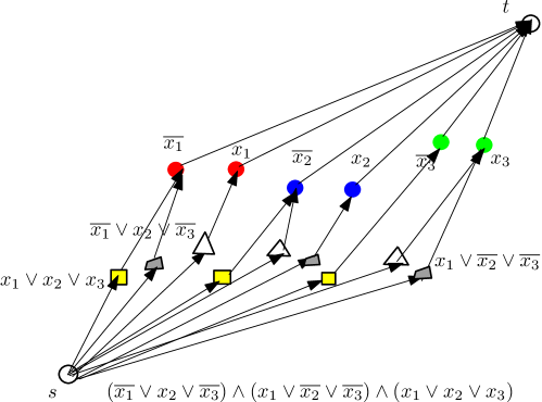
Figure 1: Illustration of the constructed directed colored graph $G$ from 3SAT. We also use different shapes for different clause vertices.

Lemma 3.1

ISCPCS is NP-hard.

The detailed proof is in the appendix, an example is given in Figure 1.

3.2 The free space diagram

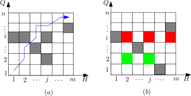
Figure 2: Illustration of the free space diagram of discrete Fréchet distance with precise input (a); and, the free space diagram of discrete Fréchet distance with imprecise input (b).

The free space diagram of the discrete Fréchet distance between a realization of $Q,H$ is composed of a grid of $n\times m$ cells, where $n$ and $m$ are the number of vertices in $Q$ and $H$ respectively. We first consider the case when both $Q,H$ are precise. In this case, let $q_{i}$ and $h_{j}$ denote the $i$-th and $j$-th vertex of $Q,H$ respectively. Each pair $(q_{i},h_{j})$ corresponds to the cell in the $i$-th row and the $j$-th column. From the definition of the discrete Fréchet distance, it corresponds to a monotone path in the grid from cell (1,1) to $(n,m)$. In the sequel, for the ease of description, we sometimes loosely call such a path “a monotone path”. We cover the details regarding such a path next.

Cell $C[i,j]=(q_{i},h_{j})$ is painted white if $d(q_{i},h_{j})\leq\epsilon$, which indicates that this cell can be passed by a potential monotone path. Cell $C[i,j]=(q_{i},h_{j})$ is painted gray if $d(q_{i},h_{j})>\epsilon$, which indicates that this grid cannot be passed by any monotone path. Each cell $C[i,j]$ could reach its monotone neighboring cell $C[i,j+1],C[i+1,j]$ or $C[i+1,j+1]$ if both of them are painted white. The discrete Fréchet distance is the minimum $\epsilon$ such that there is a path from cell (1,1) to $(n,m)$ and the path is monotone in both horizontal and vertical directions. See Figure 2 (a) for an example.

Now, we consider the free space diagram when $H=(h_{1},h_{2},...,h_{m})$ is a precise vertex sequence and $Q=(q_{1},q_{2},...,q_{n})$ is an imprecise region sequence. There are several cases below.

• (1) If $d(q,h_{j})\leq\epsilon,\forall q\in q_{i}$, then the cell $C[i,j]$ is painted white and could be passed.

• (2) If $d(q,h_{j})>\epsilon,\forall q\in q_{i}$, then the cell $C[i,j]$ is painted gray and cannot be passed.

• (3-a) There are two vertices $h_{i},h_{j}$ and an imprecise vertex $q_{k}$ satisfying either $d(q,h_{i})\leq\epsilon$ or $d(q,h_{j})\leq\epsilon,\forall q\in q_{k}$, see Figure 3(a). Then, we paint the cell $C[k,i],C[k,j]$ with the same color, which show that either $C[k,i]$ or $C[k,j]$ can be passed, see Figure 2 (b). This case will be designed as a variable gadget.

• (3-b) There are three vertices $h_{i},h_{j},h_{k}$ and an imprecise vertex $q_{x}$ satisfying
  $d(q,h_{i})\leq\epsilon$, or $d(q,h_{j})\leq\epsilon$ or $d(q,h_{k})\leq\epsilon,\forall q\in q_{x}$, see Figure 3(b). Then we paint the cell $C[x,i],C[x,j]$ and $C[x,k]$ with the same color. This case can be designed as a clause gadget. Of course, it is possible that more than one of the cells $C[x,i],C[x,j],C[x,k]$ might be passed at the same time. But our objective is to make the discrete Fréchet distance as large as possible when only one of them is passed.

In fact, there could be more complicated cases than the three cases above, but we do not need them in our construction.

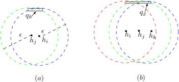
Figure 3: Illustration of the variable gadget and clause gadget.

3.3 The grid graph for the color-spanning set

The free space diagram of the discrete Fréchet distance is really a directed grid graph. Now we show how to convert the ISCPCS instance, e.g., in Figure 1, into a grid graph. The basic steps are as follows: the grid has $n+m+3$ rows and $3m+2n$ columns, and the colored cells in the grid correspond to the colored vertices in ISCPCS. The details are step by step as follows.

1. For the first row (from bottom up), all the cells are painted white, which means that all cells can be passed. The motivation is to make the starting cell (the lower-left cell $C[1,1]$, which corresponds to the start node $s$ in ISCPCS) in the grid graph reachable to all the colored clause cells (which correspond to clause vertices in ISCPCS).

2. From the 2nd row to the $(m+1)$-th row ($m$ is the number of clauses in the 3SAT instance from which the ISCPCS instance is constructed), each row has three cells with the same color. We call them clause cells, corresponding to the three clause vertices of the same color in ISCPCS. Each column has at most one clause cell. If there is a clause cell $C(k,j)$ in the $j$-th column, then the cells $C[i,j],2\leq i\leq n+1,i\neq k$, are painted white and could be passed. If there is no clause cell in the $j$-th column, then cells $C[i,j],2\leq i\leq n+1$, are painted by gray and could not be passed.

3. We do not put any clause cell in the $(m+2)$-th row. If there exists a clause cell $C[k,j]$, $2\leq k\leq n+1$, in the $j$-th column, then $C[m+2,j]$ is painted white and can be passed; otherwise, the cell $C[m+2,j]$ is painted gray and could not be passed.

4. From the $(m+3)$-th row to the $(n+m+2)$-th row ($n$ is the number of variables in the 3SAT instance from which the ISCPCS instance is constructed), each row has two cells with the same color. We call them variable cells, which correspond to two variable vertices in the ISCPCS instance. (For an example, see the cells painted with number $4$ in Figure 4.) Each column has at most one variable cell. If there is a variable cell $C[k,j]$ in the $j$-th column, then the cells $C[i,j],m+3\leq i\leq n+m+2,i\neq k$, are painted white and could be passed. If there is no variable cell in the $j$-th column, then cells $C[i,j],m+3\leq i\leq n+m+2,i\neq k$, are painted by gray and could not be passed.

5. For the last row (from bottom up), all the cells are painted white, which means that all cells can be passed. The motivation is to make sure that all the variable cells can connect to the final cell (the upper-right cell) in the grid graph, which corresponds to the destination node $t$ in ISCPCS.

6. There are a total of $(3m+2n)$ columns in the grid graph. If there are $k$ clause vertices connecting to a fixed variable vertex in ISCPCS, then there are $k$ clause cells connecting to a variable cell (say, $C[i,j]$). The $k$ clause cells are located from the $(j-k)$-th column to the $(j-1)$-th column, and the order of these columns are adjusted to make those $k$ clause cells arranged from lower-left to upper-right. (For an example, see Figure 4.) This unique design can ensure that any monotone path from $C[1,1]$ to $C[n+m+3,3m+2n]$ has to pass one clause cell and one variable cell connect to it.

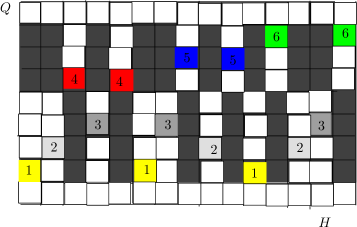
Figure 4: Illustration of the equivalence relation between the free space diagram (grid graph) and ISCPCS in Figure 1. The horizontal coordinates denote the precise points, while the vertical coordinates denote the imprecise points. A white cell means it can be passed, while the gray cell means they could not be passed, and the cells painted by the same color (and with the same number) means any one of them can be passed.

3.4 Realizing the grid graph geometrically

To complete the proof that deciding $F^{\max}(Q,H)\leq\epsilon$ is NP-hard, we need to construct a precise vertex sequence $H=(h_{1},h_{2},...,h_{3m+2n})$ and an imprecise vertex sequence $Q=(q_{1},q_{2},q_{3},...,q_{n+m+3})$ (where each imprecise vertex is modeled as a rectangle) such that the free space grid graph constructed above can be geometrically realized.

Throughout the remaining parts, let $C(a,r)$ (resp. $D(a,r)$) be a Euclidean circle (resp. disk) centered at $a$ and with radius $r$. The rectangles used to model imprecise points do not need to be along the same direction. The general idea of realizing the grid graph geometrically is as follows.

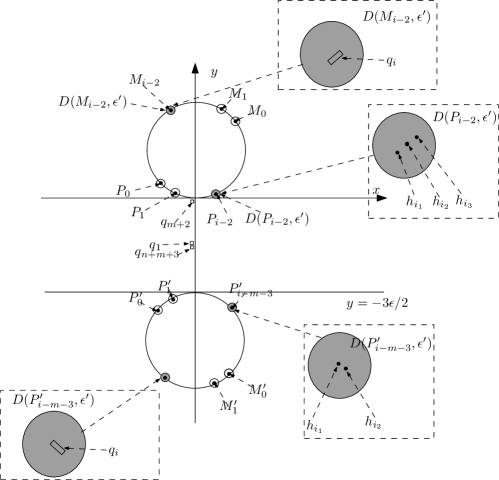
Figure 5: Illustration of the general idea of realizing the grid graph geometrically.

1. For the 2nd to the $(m+1)$-th rows of the grid graph, we design the points $P_{i}$, $M_{i},i=0,1,2,...,m-1$, which satisfy $d(P_{i},M_{i})=\epsilon$ and $d(P_{i},M_{j})\leq\epsilon-2\epsilon^{\prime}<\epsilon$ ($\epsilon^{\prime}\ll\epsilon$) when $i\neq j$. Each clause gadget is composed of three precise vertices $h_{i_{1}},h_{i_{2}},h_{i_{3}}$ ($i_{1},i_{2},i_{3}$ is the index of sequence $H$) and an imprecise vertex $q_{i}$ as in Figure 3(b). $h_{i_{1}},h_{i_{2}},h_{i_{3}}$ are located inside $D(P_{i-2},\epsilon^{\prime})$, $q_{i}$ is located inside $D(M_{i-2},\epsilon^{\prime})$ when ($2\leq i\leq m+1$). All the points $P_{i},i=0,1,2,...,m-1$ are located in a small region with diameter less than $\epsilon/10$.

2. For the $(m+3)$-th to the $(n+m+3)$-th rows, we design the points $P^{\prime}_{i}$, $M^{\prime}_{i},i=0,1,2,...,n-1$, which satisfy $d(P^{\prime}_{i},M^{\prime}_{i})=\epsilon$ and $d(P^{\prime}_{i},M^{\prime}_{j})\leq\epsilon-2\epsilon^{\prime}<\epsilon$ when $i\neq j$. Each variable gadget is composed of two precise vertices $h_{i_{1}},h_{i_{2}}$ and an imprecise vertex $q_{i}$ as in Figure 3(a). $h_{i_{1}},h_{i_{2}}$ are located inside $D(P^{\prime}_{i-m-3},\epsilon^{\prime})$, $q_{i}$ is located inside $D(M^{\prime}_{i-m-3},\epsilon^{\prime})$ when $m+3\leq i\leq n+m+2$. Again, all the points $P^{\prime}_{i},i=0,1,2,...,n-1$ are located in another small region with diameter less than $\epsilon/10$.

3. $d(P_{i},M^{\prime}_{j})>3\epsilon/2>\epsilon,d(P^{\prime}_{i},M_{j})>3\epsilon/2>\epsilon$. $d(p,q)\leq\epsilon$ when $p\in D(P_{i},\epsilon^{\prime}),q\in D(P_{j},\epsilon^{\prime}),i\neq j$, and $d(p,q)\leq\epsilon$ when $p\in D(P^{\prime}_{i},\epsilon^{\prime})$, $q\in D(P^{\prime}_{j},\epsilon^{\prime})$, and $i\neq j$.

4. For the first and last row, the first imprecise vertex $q_{1}$ and last imprecise vertex $q_{n+m+3}$ are located in a region $D((0,-3\epsilon/4),\epsilon^{\prime})$ which is fully covered by any circle $C(p,\epsilon)$ where $p\in\bigcup D(P_{i},\epsilon^{\prime})$ ($i=0,1,...,m-1$) and circle $C(p,\epsilon)$ where $p\in\bigcup D(P^{\prime}_{i},\epsilon^{\prime})$($i=0,1,...,n-1$).

5. For the $(m+2)$-th row, the vertex $q_{m+2}$ is located inide a region $D((0,0),\epsilon^{\prime})$, which is fully covered by the circle $C(p,\epsilon)$ where $p\in\bigcup D(P_{i},\epsilon^{\prime})$ ($i=0,1,...,m-1$) but not covered by any circle $C(p,\epsilon)$ where $p\in\bigcup D(P^{\prime}_{i},\epsilon^{\prime})$($i=0,1,...,n-1$).

Due to space constraints, the details for realizing the grid graph are given in the appendix (Section 7.2).

Theorem 3.2

Computing the upper bound of the discrete Fréchet-distance with imprecise input is NP-hard.

• From our construction and Lemma 1, $F^{max}(Q,H)>\epsilon$ if and only if there exist a choice that choose exactly one passable cell of each color such that there is no monotone path from lower-left cell to the upper-right cell in the equivalent free space grid graph, which holds on if and only there exist an induced subgraph $G_{s}$ consist of exactly one vertex of each color in equivalent colored graph $G$ such that in $G_{s}$ there is no monotone path from $s$ to $t$, which in turn is true if and only if the corresponding 3SAT instance is satisfiable. The total reduction time is $O((m+n)^{2})$, and the theorem is proven.       

4 The discrete Fréchet distance with shortcuts for imprecise input

As covered in the introduction, the discrete Fréchet distance is sensitive to local errors; hence, in practice, it makes sense to use the discrete Fréchet distance with shortcuts [8]. This is defined as follows. (We comment that this idea of taking shortcuts was used as early as in 2008 for simplifying protein backbones [9].)

• One-sided discrete Fréchet distance with shortcuts: For two point sequences $A=(a_{1},a_{2},a_{3},...,a_{n})$, and $B=(b_{1},b_{2},b_{3},...,b_{m})$, let $F_{c}(A,B)$ denote the discrete Fréchet distance with shortcuts on side $B$, where
  $F_{c}(A,B)=\min\{F(A,B^{\prime})\}$ and $B^{\prime}$ is a non-empty subsequence of $B$.

Alternatively, we can define the discrete Fréchet distance with shortcuts on side $B$ as follows. We loosely call each edge appearing in the set $E_{\delta}$ (in Def. 1) a match. Given a match $(a_{i},b_{j})$, the next match $(a_{k},b_{l})$ needs to satisfy one of the three conditions:

a) $k=i+1,l=j$;

b) $k=i,l>j$;

c) $k=i+1,l>j$.

In [8], Avraham et al. gave a definition of discrete Fréchet distance with shortcuts, they assumed no simultaneous jumps on both sides (i.e., case c) does not occur), though they claimed that their algorithm can be easily extended to this case when simultaneous jumps are allowed.

Now we define the discrete Fréchet distance with shortcuts for imprecise data as follows:

• $F^{\max}_{1}(U,W)$: For two region sequences $U=(u_{1},u_{2},...,u_{n})$ and $W=(w_{1},w_{2},...,w_{m})$, the upper bound of the discrete Fréchet distance with shortcuts on side $W$ is defined as $F^{\max}_{1}(U,W)=\max\{F_{c}(A,B)\}$, where $A=(a_{1},a_{2},...,a_{n})$ (resp. $B=(b_{1},b_{2},...,b_{m}$) is a possible realization of $U$ (resp. $W$) satisfying $a_{i}\in u_{i}$ and $b_{j}\in w_{j}$.

4.1 Computing $F^{\max}_{1}(U,W)$ when one sequence is imprecise

At first, we consider the case when $U$ is a precise vertex sequence composed of $n$ precise points in $R^{d}$, and $W$ is an imprecise vertex sequence, where each of the $m$ imprecise points is modeled as a ball in $R^{d}$.

Let $u^{\prime}_{i}$ denote the ball centered at $u_{i}$ with radius $\delta$, i.e., $u^{\prime}_{i}=D(u_{i},\delta)$. Let $M(i,j)$ denote the match or matching pair between $u_{i}$ and $w_{j}$.

For the discrete Fréchet distance with shortcuts on side $W$, we only need to consider the jump from $M(i,j)$ to $M(i+1,k)$ ($k\geq j$), and there is no need to consider the jump from $M(i,j)$ to $M(i,l)$($l\geq j$) . This is due to that the match $M(i,l)$ will jump to $M(i+1,l^{\prime})$ ($l^{\prime}\geq l$) finally when $i<n$, and we can jump directly from $M(i,j)$ to $M(i+1,l^{\prime})$ without passing through $M(i,l)$.

The algorithm to decide $F^{\max}_{1}(U,W)\leq\delta$ is as follows.

Starting from the starting matching pair $M(1,j^{*}(1))$ to the ending matching pair $M(n,j^{*}(n))$ if possible, where $j^{*}(1)$ is the smallest $k$ ($1\leq k\leq m$) which satisfies that $w_{k}\subseteq u^{\prime}_{1}$, $j^{*}(i)$ be the index of sequence $W$ computed by the decision procedure $F^{\max}_{1}(U,W)\leq\delta$ below for each fixed $i$, let $S$ denote the set of those matches (or matching pairs) $M(i,j^{*}(i))$.

[b] 1. $i=1,j=1$.
2. While ($i\leq n$)
            Find a smallest $k$ ($j\leq k\leq m$) which satisfies that $w_{k}\subseteq u^{\prime}_{i}$.
            If $k$ exists, let $j^{*}(i)=k$, add the match $M(i,j^{*}(i))$ to $S$,
              and update $j=k$, $i=i+1$.
            Else return $F^{\max}_{1}(U,W)>\delta$.
Return $F^{\max}_{1}(U,W)\leq\delta$.

Fig.7 The decision procedure for $F^{\max}_{1}(U,W)\leq\delta$, where $U$ is a precise sequence and $W$ is an imprecise sequence.

We will show that the above procedure correctly decides whether $F^{\max}_{1}(U,W)\leq\delta$.

Lemma 4.1

There exists a realization of $W$ to make $j^{*}(i)$ be the smallest index of sequence $W$ such that $M(i,j^{*}(i))$ is reachable by jump from $M(1,j^{*}(1))$ for each fixed $i$. That means there is no monotone increasing path from $M(1,j^{*}(1))$ to $M(i,j)$ when $1\leq j<j^{*}(i)$.

We prove this lemma by an induction on $i$.

(1) Basis: When $i=1$, then there exists a realization $(b_{1},b_{2},...,b_{j^{*}(1)-1})$ of $(w_{1},w_{2},...,w_{j^{*}(1)-1})$ respectively which satisfies $d(u_{1},b_{j})>\delta$ for $1\leq j<j^{*}(1)$. Hence, there exists a realization of $W$ which make the matching $M(1,j)$ is not reachable when $1\leq j<j^{*}(1)$.

(2) Inductive hypothesis: We assume that there exists a realization $(b_{1},b_{2},...,b_{j^{*}(k)-1})$ of $(w_{1},w_{2},...,w_{j^{*}(k)-1})$ which makes $M(k,j)$ ($1\leq j<j^{*}(k)$) not reachable when $i=k$.

(3) Inductive step: We consider the case when $i=k+1$. For $M(k+1,j)$, $j^{*}(k)\leq j<j^{*}(k+1)$ not in $S$ then there exists a realization $(b_{j^{*}(k)},...,b_{j^{*}(k+1)-1})$ of $(w_{f(k)},...,w_{j^{*}(k+1)-1})$ which satisfies $d(u_{k+1},b_{j})>\delta$, for $j^{*}(k)\leq j<j^{*}(k+1)$. Based on the inductive hypothesis, there exists a realization $(b_{1},b_{2},...,b_{j^{*}(k)})$ which makes $M(k,j)$, $1\leq j<j^{*}(k)$, not reachable. By combining the two parts, there exists a realization $(b_{1},b_{2},...,b_{j^{*}(k)},...,b_{j^{*}(k+1)-1})$ of $(w_{1},w_{2},...,w_{j^{*}(k)},...,w_{j^{*}(k+1)-1})$ which makes $M(k+1,j)$, where $1\leq j<j^{*}(k+1)$, not reachable.       

Lemma 4.2

In ${\mathbb{R}}^{d}$, given a precise vertex sequence $U$ with size $n$ and an imprecise vertex sequence $W$ with size $m$ (each modeled as a $d$-ball), whether $F^{\max}_{1}(U,W)\leq\delta$ can be determined in $O(d(n+m))$ time and space.

• If the above decision procedure returns “$F^{\max}_{1}(U,W)>\delta$” when $i=k+1$, then there exists a realization of $W$ to make $M(k+1,j)$ not reachable, for $k+1<n$ and $j^{*}(k)\leq j\leq m$, based on Lemma 4.1. That means $F^{\max}_{1}(U,W)>\delta$.

  If the above decision procedure returns “$F^{\max}_{1}(U,W)\leq\delta$”, then there exists a monotone path from $M(1,j^{*}(1))$ to $M(n,j^{*}(n))$ for any realization of $W$. The reason is that, for any $i$ and $j^{*}(i)$, $M(i,j^{*}(i))\in S$ implies $w_{j^{*}(i)}\subseteq u^{\prime}_{i}$, which means $F^{\max}_{1}(U,W)\leq\delta$. The correctness is hence proven.

  As for the running time, checking whether $w_{j}\subseteq u^{\prime}_{i}$ takes $O(d)$ time. The decision procedure incrementally tests on a row- and column-monotone path. Therefore, it runs in $O(d(m+n))$ time and space.       

Let $\delta_{i,j}=d(u_{i},c_{j})+r_{j}$ where $c_{j}$ and $r_{j}$ are the center and radius of $w_{j}$ respectively. For the optimization problem, there are a total of $O(mn)$ events when $\delta$ increases continuously. Here, an event $w_{j}\subseteq u^{\prime}_{i}$ occurs when $\delta$ increases to $\delta_{ij}$. Therefore, we can solve the optimization problem of computing $F^{\max}_{1}(U,W)$ in $O(dmn\log mn)$ time by sorting $\delta_{i,j}$’s and performing a binary search. We show how to improve this bound below. We first consider the planar case in the next theorem.

Theorem 4.3

In ${\mathbb{R}}^{2}$, given a precise vertex sequence $U$ with size $n$ and an imprecise vertex sequence $W$ with size $m$, all modeled as disks in ${\mathbb{R}}^{2}$ with an equal radius, $F^{\max}_{1}(U,W)$ can be computed in $O((m^{2/3}n^{2/3}+m+n)\log^{3}(m+n))$ time.

• The event $w_{j}\subseteq u^{\prime}_{i}$ occurs when $\delta=\delta_{i,j}$. We do not need to sort the $O(mn)$ distances; instead, we can use the distance selection algorithm in [19] as follows. One can select the $k$-th smallest pairwise distance $d_{k}$ in $A\times B$, where $A$ and $B$ are two precise vertex sequences in the plane and $|A|=n,|B|=m$. The running time of this distance selection algorithm is $O((m^{2/3}n^{2/3}+m+n)\log^{2}(m+n))$ [19]. By combining this distance selection algorithm and the binary search, we can compute $F^{\max}_{1}(U,W)$ in $O((m+n)\log(mn)+(m^{2/3}n^{2/3}+m+n)\log^{2}(m+n)\log(mn))$ $=O((m^{2/3}n^{2/3}+m+n)\log^{3}(m+n))$ time.       

Unfortunately, the distance selection algorithm could not be extended to high dimensional space. Hence, in a dimension higher than two, we use a dynamic programming method to compute $F^{\max}_{1}(U,W)$.

Let $U(i,j)$ (resp. $W(i,j)$) denote the partial sequence $U(i,j)=(u_{i},u_{i+1},...,u_{j})$ (resp. $W(i,j)=(w_{i},w_{i+1},...,w_{j}))$. $F^{\max}_{1}(i,j)$ denotes the upper bound of the discrete Fréchet distance with shortcuts on side $W(1,j)$ for sequences $U(1,i)$ and $W(1,j)$, and $Z^{\max}_{1}(i,j)$ denotes the upper bound of the discrete Fréchet distance with shortcuts on side $W(1,j)$ between $U(1,i)$ and $W(1,j)$ on the condition that $w_{j}$ is retained (not cut), that means $w_{j}$ match $u_{i}$, namely $Z^{\max}_{1}(i,j)=\max\{F^{\max}_{1}(i-1,j),\delta_{i,j}\}$. While in $F^{\max}_{1}(i,j)$, $u_{i}$ may do not match $w_{j}$ as $w_{j}$ may be cut.

Then we have the recurrence relations as follows.

$$Z^{\max}_{1}(i+1,j)\\ =\left\{\begin{array}[]{ll}\max\{F^{\max}_{1}(i,j),\delta_{i+1,j}\},&\mbox{$i>0$}\\ \delta_{1,j},&\mbox{$i=0$}\end{array}\right.$$

$$F^{\max}_{1}(i,j+1)\\ =\left\{\begin{array}[]{ll}\min\{F^{\max}_{1}(i,j),Z^{\max}_{1}(i,j+1)\},&\mbox{$j>0$}\\ Z^{\max}_{1}(i,j+1),&\mbox{$j=0$}\end{array}\right.$$

We need to run these two recurrence relations alternatively, e.g. computing $Z^{\max}_{1}(i,*)$ ($(i,*)$ denotes $\{(i,j),1\leq j\leq m\}$), then $F^{\max}_{1}(i,*)$, then $Z^{\max}_{1}(i+1,*)$, etc. It is easy to see that this dynamic programming algorithm takes $O(mn)$ time and space after all the distances $\delta_{i,j}$ are calculated in $O(dmn)$ time and space. On the other hand, the space complexity can be improved as we only need to store a constant number of columns of values and compute $\delta_{i,j}$ when needed. Hence we have the following theorem.

Theorem 4.4

In ${\mathbb{R}}^{d}$, given a precise vertex sequences $U$ of size $n$ and an imprecise vertex sequences $W$ of size $m$ (each modeled as a $d$-ball), $F^{max}_{1}(U,W)$ can be computed in $O(dmn)$ time and $O(d(m+n))$ space.

4.2 Computing $F^{\max}_{1}(U,W)$ when both sequences are imprecise

In this subsection, we consider the problem of computing $F^{\max}_{1}(U,W)$ when both $U=(u_{1},u_{2},...,u_{n})$ and $W=(w_{1},w_{2},...,w_{m})$ are imprecise sequences, where each vertex is modeled as a disk in ${\mathbb{R}}^{2}$. (Our algorithm works in ${\mathbb{R}}^{d}$, but as it involves Voronoi diagram in ${\mathbb{R}}^{d}$, the high cost makes it impractical.)

For two imprecise sequences $U,W$, and a precise point $p$, the maximal distance between a precise point $p$ and a region $w_{x}$ is defined as $D_{\max}(p,w_{x})=\max\{d(p,q),q\in w_{x}\}$. Let $D_{\min}(p,j,k)=\min_{j\leq x\leq k}\{D_{\max}(p,w_{x})\}$ denote the minimal distance between a point $p$ and several regions $\{w_{j},w_{j+1},...,w_{k}\}$.

We define $D(i,j,k)=\max\{D_{\min}(p,j,k),p\in u_{i}\}$. In this subsection, we compute the $j^{*}(i)$ by using the decision procedure below:

[b] 1. $i=1,j=1$.
2. While ($i\leq n$)
            Find a smallest $k$ ($j\leq k\leq m$) which satisfies $D(i,j,k)\leq\delta$.
            If $k$ exists, let $j^{*}(i)=k$, add $M(i,j^{*}(i))$ to $S$,
               and update $j=k$, $i=i+1$.
            Else return $F^{\max}_{1}(U,W)>\delta$.
Return $F^{\max}_{1}(U,W)\leq\delta$.

Fig. 8 The decision procedure for $F^{\max}_{1}(U,W)\leq\delta$ when both $U$ and $W$ are imprecise sequences.

Lemma 4.5

Given two imprecise vertex sequences $U$ and $W$ with sizes $|U|=n$ and $|W|=m$, each vertex modeled as a disk in ${\mathbb{R}}^{2}$), $F^{\max}_{1}(U,W)\leq\delta$ can be determined in $O(m^{2}+n)$ time and $O(m+n)$ space.

• The correctness is given as follows.

  (1) If the decision procedure returns “$F^{max}_{1}(U,W)>\delta$”, then there exists a realization of $U$ and $W$ which makes it impossible to reach the last matching pair $M(n,j^{*}(n))$. The argument is similar to Lemma 4.1 and omitted here. That means $F^{max}_{1}(U,W)>\delta$.

  (2) If the decision procedure returns “$F^{max}_{1}(U,W)\leq\delta$”, then $S$ has $n$ elements, i.e., $S=\{M(1,j^{*}(1))$, $M(2,j^{*}(2))$, $M(3,j^{*}(2))$,…,$M(n,j^{*}(n))\}$, where $j^{*}(i)\leq j^{*}(i+1)$. We claim that there exists monotone matching pair set $\{M(i,j(i))|1\leq i\leq n\}$ ($j(i)\leq j^{*}(i)$) under any realization of $U$ and $W$, where $j(i)$ is an index of W and $u_{i}$ match $w_{j(i)}$ and $j(i)\leq j(i+1)$.

  We prove the claim by an induction on $i$.

  (2.1) Basis: When $i=1$, if all the matching pairs $M(1,j)$, $j\leq j^{*}(1)$, are not reachable, then there exists a realization $b_{x},1\leq x\leq j^{*}(1)$, and $a_{1}$ which satisfy $d(a_{1},b_{x})>\delta$. Then $D(1,1,j^{*}(1))>\delta$, and we have a contradiction, that means there exist $j(1)\leq j^{*}(1)$ such that $M(1,j(1))$ is possible under any realization.

  (2.2) Inductive hypothesis: We assume that the claim holds when $i=l$.

  (2.3) Inductive step: Now we consider the case when $i=l+1$. By the inductive hypothesis, there exists monotone matching set $M(1,j(1)),M(2,j(2)),...,M(l,j(l))$, $j(i)\leq j^{*}(i)$ under any realization of $U(1,l),W(1,j)$. As $D(l+1,j,j^{*}(l+1))\leq D(l+1,j^{*}(l),j^{*}(l+1))\leq\delta$, there exists a matching pair $M(l+1,j(l+1))$, where $j(l+1)\leq j^{*}(l+1)$, which is reachable by jumping directly from $M(l,j(l))$ under any realization of $U(l+1,l+1)$ and $W(j+1,j(l+1))$. Hence, if the decision procedure returns “$F^{max}_{1}(H,Q)\leq\delta$”, then $F^{max}_{1}(H,Q)\leq\delta$.

We now compute the time it takes to find a smallest $k$ ($j\leq k\leq m$) satisfying $D(i,j,k)\leq\delta$. The steps to compute $D(i,j,k)$ can be done as follows.

(I) We compute the inverted additive Voronoi Diagram [21] (iaVD) of imprecise vertices $w_{j},w_{j+1},...,w_{k}$ modeled as disks (may have different sizes), which takes $O((k-j)\log(k-j))$ time.

(II) If the imprecise region $u_{i}$ intersects the boundary of iaVD, then some vertex of the partial boundary within $u_{i}$ would be the realization of $u_{i}$ in computing $D(i,j,k)$. Otherwise, the imprecise region $u_{i}$ is located in the cell controlled by some site $w_{x}$. Then, the diameter of the region $u_{i}\cup w_{x}$ would be $D(i,j,k)$. This step takes $O(k-i)$ time.

As we need to construct the inverted additive Voronoi Diagram incrementally, each single insertion takes $O(s)$ time, where $s$ is the size of the iaVD. Hence the total time to find a smallest $k$ ($j\leq k\leq m$) is $\sum_{j\leq x\leq k}(x-j)=O((k-j)^{2})$. Therefore, the total time complexity is $\sum_{1\leq i\leq n}(j^{*}(i+1)-j^{*}(i))^{2}=O(m^{2}+n)$.       

For the optimization problem, we again use a dynamic programming algorithm to solve it. The algorithm is similar to that in Theorem 4.4 and the difference is to use $D(i,j,k)$ instead of $\delta_{i,j}$. The recurrence relation is as follows.

$$F^{\max}_{1}(i+1,k)\\ =\left\{\begin{array}[]{ll}\min_{1\leq j\leq k}\{\max\{F^{\max}_{1}(i,j),D(i+1,j,k)\}\},&\mbox{$i>0$}\\ D(1,1,k),&\mbox{$i=0$}\end{array}\right.$$

It seems that the dynamic programming algorithm takes $O(nm^{2})$ time after all the distances $D(i,j,k)$ are calculated in $O(nm^{3})$ time. However, we can use the Monge property to speed up the computation of dynamic programming, we only need to compute $O(nm)$ distances $D(i,j,k)$’s in $O(nm^{2})$ time.

(1) $F^{\max}_{1}(i,j)$ is a monotone decreasing function when $j$ increases for a fixed $i$.

(2) $D(i+1,j,k)$ is a monotone increasing function when $j$ increases for fixed $i$ and $k$.

(3) Let $j_{k}$ denote the index satisfying $F^{\max}_{1}(i+1,k)=\max\{F^{\max}_{1}(i,j_{k}),D(i+1,j_{k},k)\}$, and $j_{k+1}$ denote the index satisfying $F^{\max}_{1}(i+1,k+1)=$ $\max\{F^{\max}_{1}(i,j_{k+1})$, $D(i+1,j_{k+1},k+1)\}$, then $j_{k+1}\geq j_{k}$.

Hence we only need to try distances $D(i+1,j_{k},k+1),D(i+1,j_{k}+1,k+1),D(i+1,j_{k}+2,k+1),...,D(i+1,j_{k+1},k+1),D(i+1,j_{k+1}+1,k+1)$ when computing $F^{\max}_{1}(i+1,k+1)$ for a fixed $i$ and $k$, namely $(j_{k+1}-j_{k}+2)$ distances, hence the total number of distance is $O(m)$ for a fixed $i$.

Hence $F^{\max}_{1}(i+1,k)$ ($1\leq k\leq m$) can be calculated in $O(m)$ time after the distances $D(i+1,j,k)$ ($1\leq k\leq m$) are calculated for a fixed $i$. We then only need to try $O(m)$ distances $D(i+1,j,k)$ ($1\leq k\leq m$): the update of iaVD needs at most $O(m)$ insert operations, $O(m)$ deletion operations, and $O(m)$ query operations, each takes at most $O(m)$ time. Hence the total time is $O(m^{2})$ for a fixed $i$. Hence we have the theorem below.

Theorem 4.6

In ${\mathbb{R}}^{2}$, given two imprecise sequences $U$ and $W$ of size $n$ and $m$ respectively, where each imprecise vertex is modeled as a disk, $F^{max}_{1}(U,W)$ can be computed in $O(nm^{2})$ time.

We comment that when both $U$ and $W$ are imprecise, our algorithm could still work in ${\mathbb{R}}^{d}$. But due to the high cost (like constructing the $d$-dimensional Voronoi diagram), the algorithm then becomes impractical. Hence, we only focus on the problem in ${\mathbb{R}}^{2}$ for this case.

5 Concluding remarks

In this paper, we consider the problem of computing the discrete Fréchet distance of imprecise input. We address the open problem posed by Ahn [3, 4] et al. a few years ago, and show that the discrete Fréchet distance upper bound problem of imprecise data is NP-hard. And our NP-hardness proof is quite complicate, the construction has a combinatorial and a geometric part. In the combinatorial part, we interpret the imprecise discrete distance in terms of finding monotone paths through a colored grid graph; In the geometric part, we show that the relevant colored free space diagram grids can be realized geometrically. Given two imprecise vertex sequence $U,W$ (each vertex modeled as a $d$-dimensional ball), we show that the upper bound of the discrete Fréchet distance between $U$ and $W$ can be computed in polynomial time if allowing shortcuts on one side. It would be interesting to consider these problems under the continuous Fréchet distance.

6 Acknowledgments

CF’s research is supported by the Benjamin PhD Fellowship. BZ’s research is supported by the Open Fund of Top Key Discipline of Computer Software and Theory in Zhejiang Provincial Colleges at Zhejiang Normal University.

7 Appendix

7.1 Proof of Lemma 1

• Let $\phi$ be a Boolean formula in conjunctive normal form with $n$ variables $x_{1}$, $x_{2}$, $\ldots,x_{n}$ and $m$ clauses $C_{1}$, $C_{2}$, $\ldots,C_{m}$, each of size at most three. We take the following steps to construct an instance $G$ of ISCPCS.

  For each Boolean variable $x_{i},\overline{x_{i}}$ in $\phi$, we use two vertices with the same color (and different variables always use different colors), one denoted as $x_{i}$, the other denoted as $\overline{x_{i}}$. See $x_{1}$, $x_{2}$, and $x_{3}$ in Figure 1 for example. Eventually, we have to pick one of the two vertices to retain this color. One represents that the variable $x_{i}$ is assigned the True value, and the other corresponds to the value False.

  For each clause $C_{i}$ in $\phi$, we construct three vertices with the same color (which has never used before). (We use shapes instead of colors in Figure 1 to emphasize the difference with variables; for example, we use three triangular vertices in Figure 1 to denote clause $(\overline{x_{1}}\vee x_{2}\vee\overline{x_{3}})$). We then add directed edges between the clause vertices and variable vertices, the rule is as follows: let vertex $p_{i}$ be the vertex used to denote variable $\overline{x_{i}}$ (resp. $x_{i}$), and vertex $c_{i,j}$ be the vertex used to denote the clause $C_{j}$ which contains $x_{i}$ (resp. $\overline{x_{i}}$), then we add a directed edge from $c_{i,j}$ to $p_{i}$, see Figure 1.

  At last we add edges from the source $s$ to each vertex denoting a clause, and add edges from each vertex denoting a variable to the destination $t$. It is easy to ensure that there is no crossing between the edges: all the vertices denoting variables are arranged from left to right, there is a clause vertices for each literal (variable vertex), and each of the clause vertices connecting to a fixed variable vertex $x_{i}$ is just below the variable vertices $x_{i}$. Let the resulting directed geometric graph be $D$. We next complete the proof by proving that $\phi$ is satisfiable iff there exists an induced subgraph $G_{s}$ such that in $G_{s}$ there is no path from $s$ to $t$.

  ‘$\rightarrow$’ If $\phi$ is satisfiable with some truth assignment, then there is at least one true literal in each clause $C_{i}$. We show how to compute the induced subgraph $G_{s}$ from $G$ as follows. For each pair of variable vertices representing $\{x_{j},\overline{x_{j}}\}$, we pick one which is assigned True. Let $C_{i}=u\vee v\vee w$, where $u,v,w$ are literals in the form of $x_{j}$ or $\overline{x_{j}}$. Then we have three clause vetices $c_{u,i},c_{v,i}$ and $c_{w,i}$, of the same color $color_{i}$, representing the clause $C_{i}$. WLOG, just suppose that $u$ is a true literal in $C_{i}$ (pick any one true literal if there exist more than one literal in $C_{i}$ be true), and we choose the vertex $c_{u,i}$ to cover the color $color_{i}$. By construction, in $D$, there is no edge from the vertex $c_{u,i}$ to the vertex $p_{u}$ representing $u$. Hence, there is no path from $s$ to $t$ crossing the clause vertex $c_{u,i}$ (representing clause $C_{i}$). As this holds for all clauses and any path from $s$ to $t$ has to pass a clause vertex, hence there exists an induced subgraph $G_{s}$ consist of exactly one vertex of each color with no path from $s$ to $t$.

  ‘$\leftarrow$’ If there exists an induced subgraph $G_{s}$ consist of exactly one vertex of each color with no path from $s$ to $t$, we need to prove that $\phi$ is satisfiable. Suppose to the contrary that $\phi$ is not satisfiable, then at least one clause is not satisfiable. Let this clause be $C_{i}=u\vee v\vee w$, and let the clause vertices $c_{u,i}$, $c_{v,i}$ and $c_{w,i}$ connect to the variable vertices $p_{u}$, $p_{v}$ and $p_{w}$ in $D$ which correspond to the variables $\overline{u}$, $\overline{v}$, $\overline{w}$ respectively. As $u$, $v$ and $w$ are all false, $p_{u}$, $p_{v}$, $p_{w}$ are all picked in the induced subgraph. Then, there exists a path from $s$ to $t$ passing through $c_{u,i}$, $c_{v,i}$ or $c_{w,i}$, as one of them must be picked. A contradiction!

  Hence, $\phi$ is satisfiable if and only if there exists an induced subgraph $G_{s}$ consist of exactly one vertex of each color with no path from $s$ to $t$. The reduction obviously takes $O(n+m)$ time.       

7.2 Details for realizing the grid graph geometrically

The details for realizing the grid graph are given here. First, we create the points used for determining the position of the vertices in $H$ and $Q$. Let $\theta$ be satisfying that $\max\{m,n\}*\theta\leq\pi/20$. Let $N=\max\{m,n\}$, and WLOG, let $N$ be even. We construct a circle $C(O,r)$, where $O=(0,\epsilon/2)$ and $r=\epsilon/2$.

Figure 6: Illustration of the position of points $P_{i}$’s and $M_{i}$’s.

We construct a sequence of points $P_{i}$ ($i=0,1,2,...,N$) on the lower half of circle $C(O,r)$ in counterclockwise order, and the point $P_{N/2}$ overlaps with point $(0,0)$, see Figure 6. Note that the distance between two adjacent points $P_{i}$ and $P_{i+1}$ is $L=2\frac{\epsilon}{2}\sin\frac{\theta}{2}=\epsilon\sin\frac{\theta}{2}$, and $\angle P_{i}OP_{i+1}=\theta$, for $i=0,1,2,...,N-1$. Hence, all the points $P_{i},i=0,1,2,...,N$ are within a region of diameter less than $\frac{\pi}{20}\cdot\frac{\epsilon}{2}<\epsilon/10$. (We comment that in Figure 6, these points are spread out much more than they should be, as we need the space for putting the labels.)

We then construct a sequence of points $M_{i}$ ($i=0,1,2,...,N$) on the upper half of circle $C(O,r)$ in counterclockwise order. Each line $\overline{P_{i}M_{i}}$ crosses the center of $C(O,r)$; namely $M_{i}$ is the symmetry of the point $P_{i}$ about point $O$.

It is obvious that $d(M_{i},P_{i})=\epsilon$ and $d(M_{i},P_{j})<\epsilon,i\neq j$. Recall that $D(P_{i},\epsilon^{\prime})$ is the neighborhood (disk) centered at $P_{i}$ with radius be $\epsilon^{\prime}$. Here, we have $\epsilon^{\prime}=\frac{1}{2}\min\{\epsilon-d(P_{i},M_{j}),i\neq j\}$; moreover, $d(p,q)\leq(\epsilon-2\epsilon^{\prime})+2\epsilon^{\prime}\leq\epsilon$, for $p\in D(P_{i},\epsilon^{\prime})$, $q\in D(M_{j},\epsilon^{\prime})$, and $i\neq j$.

Let $P^{\prime}_{i}$ be the symmetry of the point $P_{i}$ along the horizontal line $y=-3\epsilon/4$. Let $M^{\prime}_{i}$ be the symmetry of the point $M_{i}$ along the horizontal line $y=-3\epsilon/4$. We finish the steps of our construction in order as follows.

Figure 7: Illustration of the deployment of vertices of $P_{i}$’s and $Q$, corresponding to Figure 4.

1. The imprecise vertices $\{q_{2},...,q_{m+1}\}$ used to construct the clause gadget are deployed in the upper half of the circle $C((0,\frac{\epsilon}{2}),\frac{\epsilon}{2})$. An example is given in Figure 7 (see $q_{2},q_{3},q_{4}$ there). For an imprecise vertex $q_{i},2\leq i\leq m+1$, three points $h_{i_{1}},h_{i_{2}},h_{i_{3}}$ are located in $D(P_{i-2},\epsilon^{\prime})$, $q_{i}$ is located in $D(M_{i-2},\epsilon^{\prime})$, and the three circles $C(h_{i_{1}},\epsilon),C(h_{i_{2}},\epsilon),C(h_{i_{3}},\epsilon)$ cover $q_{i}$ as in Figure 8. The clause gadget is constructed as follows. The point $h_{i_{2}}$ overlaps with $P_{i}$, $h_{i_{1}}$ is located to the left of line $\overline{P_{i-2}M_{i-2}}$ with a distance $\epsilon^{\prime}/3$ to $h_{i_{2}}$, and $h_{i_{3}}$ is located to the right of line $\overline{P_{i-2}M_{i-2}}$ with a distance $\epsilon^{\prime}/3$ to $h_{i_{2}}$. The points $h_{i_{1}},h_{i_{2}},h_{i_{3}}$ are located on the same line perpendicular to line $\overline{P_{i-2}M_{i-2}}$. The three intersections between $C(h_{i_{1}},\epsilon),C(h_{i_{2}},\epsilon),C(h_{i_{3}},\epsilon)$ are $s_{1},s_{2},s_{3}$ from left to right about the horizontal line $\overline{h_{i_{1}}h_{i_{3}}}$. Let $q_{i}$ be the rectangle with length $2\epsilon^{\prime}/3$ and width $\epsilon^{\prime\prime}$, the upper long side of $q_{i}$ crosses $s_{1},s_{3}$ and is symmetric along the line $P_{i-2}M_{i-2}$, and the lower long side of $q_{i}$ crosses $s_{2}$. $\epsilon^{\prime\prime}<d(s_{2},M_{i-2})=\epsilon-\sqrt{\epsilon^{2}-(\epsilon^{\prime}/3)^{2}}<\epsilon^{\prime}/3$. Hence $d(M_{i-2},q)<\epsilon^{\prime}$ when $q\in q_{i}$.

   The imprecise vertices $\{q_{j}|2\leq j\leq m+1,j\neq i\}$ are fully covered by $C(h_{i_{1}},\epsilon)$, $C(h_{i_{2}},\epsilon)$, $C(h_{i_{3}},\epsilon)$ as $d(p,q)<\epsilon$, $p\in D(P_{i},\epsilon^{\prime}),q\in D(M_{j},\epsilon^{\prime}),i\neq j$. The above design can ensure that, in the corresponding free space grid graph, either one of the three cells $C[i,i_{1}],C[i,i_{2}],C[i,i_{3}]$ can be passed by a potential monotone path, and the cells $C[i,j_{1}],C[i,j_{2}],C[i,j_{3}],j\neq i,$ can also be passed ($h_{j_{1}},h_{j_{2}},h_{j_{3}}$ and $q_{j}$, $j\neq i$, are used to construct another clause gadget), while the rest of cells in the $i$-th row cannot be passed.

2. The imprecise vertices $\{q_{m+3},...,q_{n+m+2}\}$ used to construct the variable gadgets are deployed in the lower half of another circle $C((0,-2\epsilon),\frac{\epsilon}{2})$. For an example, see Figure 7. For an imprecise vertex $q_{i},m+3\leq i\leq n+m+2$, two points $h_{i_{1}},h_{i_{2}}$ are located in $D(P^{\prime}_{i-m-3},\epsilon^{\prime})$, $q_{i}$ is located in $D(M^{\prime}_{i-m-3},\epsilon^{\prime})$ and the long side of $q_{i}$ is parallel to the tangent line at $M^{\prime}_{i-n-3}$. Two circles $C(h_{i_{1}},\epsilon),C(h_{i_{2},\epsilon})$ cover $q_{i}$ as in Figure 3(a) to construct a variable gadget. The other imprecise vertices $\{q_{j}|m+3\leq j\leq n+m+2,j\neq i\}$ are fully covered by $C(h_{i_{1}},\epsilon),C(h_{i_{2}},\epsilon)$, the precise location is similar to the construction in Figure 8. This design can ensure that, in the corresponding free space grid graph, one of the cells $C(i,i_{1}),C(i,i_{2})$ can be passed by a potential monotone path, and the cells $C(i,j_{1}),C(i,j_{2}),j\neq i$ can also be passed ($h_{j_{1}},h_{j_{2}}$ and $q_{j}$ are used to construct another variable gadget), but the other cells in the $i$-th row cannot be passed.

3. The first imprecise vertex $q_{1}$ and last imprecise vertex $q_{n+m+3}$ are deployed in $D((0,-3\epsilon/4),\epsilon^{\prime})$, which are fully covered by all the circles $C(p,\epsilon),p\in\bigcup D(P_{i},\epsilon^{\prime})$ or $p\in\bigcup D(P^{\prime}_{i},\epsilon^{\prime})$, as $(\frac{\epsilon}{10}+\frac{3\epsilon}{4}+2\epsilon^{\prime})<\epsilon$. This design can ensure that, in the corresponding free space grid graph, all the cells in the first row and last row can be passed by a potential monotone path.

4. The imprecise vertex $Q_{m+2}$ is deployed inside region $D((0,0),\epsilon^{\prime})$, which is only fully covered by any circle $C(p,\epsilon),p\in\bigcup D(P_{i},\epsilon^{\prime})$ . But it is not covered by the circle $C(p,\epsilon),p\in\bigcup D(P^{\prime}_{i},\epsilon^{\prime})$. This design above can ensure that, in the corresponding free space grid graph, all the cells $C[m+2,i_{1}],C[m+2,i_{2}],C[m+2,i_{3}]$ in the $m+2$-th row can be passed ($h_{i_{1}},h_{i_{2}},h_{i_{3}}$ are used to construct the clause gadget with $q_{i}$), while the other cells in the $(m+2)$-th row cannot be passed.

5. At last, we adjust the order and rename for the vertices in $H$. If there is a variable cell in the $j$-th row of the free space grid graph, and there are a total of $k$ clause cells connecting to it, say the row number of $k$ cells are $1^{\prime},2^{\prime},...,i^{\prime},...,k^{\prime}$ respectively, then we choose one point (never be renamed before) from the three points $h_{i^{\prime}_{1}},h_{i^{\prime}_{2}},h_{i^{\prime}_{3}}$ for each fixed $i^{\prime}$, and rename those $k$ points as $h_{j-k},h_{j-k+1},...,h_{j-1}$ in order.

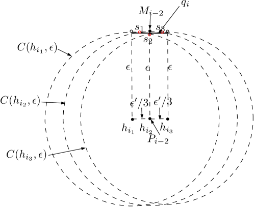
Figure 8: Illustration of the precise location of $h_{i_{1}},h_{i_{2}},h_{i_{3}}$ and $q_{i}$.

References

- [1] M. Abellanas, F. Hurtado, C. Icking, R. Klein, E. Langetepe, L. Ma, B. Palop, and V. Sacristan. Smallest color-spanning objects. Proc. 9th European Sympos. Algorithms (ESA’01), pp. 278–289, 2001.
- [2] P. Agarwal, R. Avraham, H. Kaplan, and M. Sharir. Computing the discrete Fréchet distance in subquadratic time. SIAM J. Comput., 43(2):429-449, 2014.
- [3] H-K. Ahn, C. Knauer, M. Scherfenberg, L. Schlipf, and A. Vigneron. Computing the discrete Fréchet distance with imprecise input. In Proc. ISAAC’10, pp. 422-433, 2010.
- [4] H-K. Ahn, C. Knauer, M. Scherfenberg, L. Schlipf, and A. Vigneron. Computing the discrete Fréchet distance with imprecise input. Int. J. Comput. Geometry Appl., 22(1):27-44, 2012.
- [5] H. Alt and M. Buchin. Semi-computability of the Fréchet distance between surfaces. In Proc. EuroCG’05, pp. 45-48, 2005.
- [6] H. Alt, A. Efrat, G. Rote, and C. Wenk. Matching planar maps. In Proc. SODA’03, pp. 589-598, 2003.
- [7] H. Alt and M. Godau. Computing the Fréchet distance between two polygonal curves. Int. J. Comput. Geometry Appl., 5:75-91, 1995.
- [8] R. Avraham, O. Filtser, H. Kaplan, M. Katz, and M. Sharir. The discrete Fréchet distance with shortcuts via approximate distance counting and selection. In Proc. SoCG’14, pages 377, 2014.
- [9] S. Bereg, M. Jiang, W. Wang, B. Yang, and B. Zhu. Simplifying 3D polygonal chains under the discrete Fréchet distance. In Proc. 8th Latin American Theoretical Informatics Sympos. (LATIN’08), pp. 630–641, 2008.
- [10] S. Brakatsoulas, D. Pfoser, R. Salas, and C. Wenk. On map-matching vehicle tracking data. In Proc. the 31st International Conf. on Very Large Data Bases (VLDB’05), pp. 853-864, 2005.
- [11] K. Buchin, M. Buchin, and C. Wenk. Computing the fréchet distance between simple polygons. Comput. Geom. Theory Appl., 41(1-2):2-20, 2008.
- [12] S. Das, P. Goswami, and S. Nandy. Smallest Color-Spanning Object Revisited. Int. J. Comput. Geometry Appl, 19(5):457-478, 2009.
- [13] A. Driemel and S. Har-Peled. Jaywalking your dog: Computing the Fréchet distance with shortcuts, SIAM J. Comput., 42(5):1830-1866, 2013.
- [14] T. Eiter and H. Mannila. Computing discrete fréchet distance. Technical report, Technische Universitat Wien, 1994.
- [15] C. Fan, O. Filtser, M. Katz, T. Wylie, and B. Zhu. On the chain pair simplification problem. In Proc. WADS’15, LNCS 9214, pp. 351-362, 2015.
- [16] C. Fan, J. Luo, and B. Zhu. Fréchet-distance on road networks. In Proc. CGGA’10, LNCS 7033, pp. 61-72, 2011.
- [17] M. Jiang, Y. Xu, and B. Zhu. Protein structure-structure alignment with discrete Fréchet distance. J. Bioinfo. and Comput. Biology, 6(1):51-64, 2008.
- [18] W. Ju, J. Luo, B. Zhu, and O. Daescu. Largest area convex hull of imprecise data based on axis-aligned squares. J. Comb. Optim., 26(4):832–859, 2013.
- [19] M. J. Katz and M. Sharir. An expander-based approach to geometric optimization, SIAM J. Comput., 26(5):1384-1408, 1997.
- [20] A. A.Khanban and A. Edalat. Computing Delaunay triangulation with imprecise input data. In Proc. 15th Canadian Conference on Computational Geometry (CCCG’03), pp. 94-97, 2003.
- [21] C. Knauer, M. Löffler, M. Scherfenberg, and T.Wolle. The directed Hausdorff distance between imprecise point sets. In Proc. ISAAC’09, LNCS 5878, pp. 720-729, 2009.
- [22] M. Löffler and J. Snoeyink. Delaunay triangulation of imprecise points in linear time after preprocessing. Comput. Geom. Theory Appl., 43(3):234-242, 2010.
- [23] M. Löffler and M.J. van Kreveld. Largest and smallest tours and convex hulls for imprecise points. In Proc. SWAT’06, LNCS 4059, pp. 375-387, 2006.
- [24] A. Maheshwari, J. Sack, K. Shahbaz, and H. Zarrabi-Zadeh. Fréchet distance with speed limits. Comput. Geom. Theory Appl., 44(2):110-120, 2011.
- [25] A. Maheshwari, J. Sack, K. Shahbaz, and H. Zarrabi-Zadeh. Staying close to a curve. Proc. CCCG’11, pp. 55-58, 2011.
- [26] G. Rote. Computing the Fréchet distance between piecewise smooth curves. Comput. Geom. Theory Appl., 37(3):162-174, 2007.
- [27] J. Sember and W. Evans. Guaranteed Voronoi diagrams of uncertain sites. In Proc. CCCG’08, 2008.
- [28] T. Wylie and B. Zhu. Protein chain pair simplification under the discrete Fréchet distance, IEEE/ACM Trans. Comput. Biology Bioinform., 10(6):1372-1383, 2013.
- [29] T. Wylie and B. Zhu. Following a curve with the discrete Fréchet distance. Theoretical Computer Science, 556:34-44, 2014.
- [30] B. Zhu. Protein local structure alignment with discrete Fréchet distance. J. of Comput. Biology, 14(10):1343-1351, 2007.