Pseudo energy wells in active systems

Abstract

Active stabilization in systems with zero or negative stiffness is an essential element of a wide variety of biological processes. We study a prototypical example of this phenomenon at a micro-scale and show how active rigidity, interpreted as a formation of a pseudo-well in the effective energy landscape, can be generated in an overdamped ratchet-type stochastic system. We link the transition from negative to positive rigidity with correlations in the noise and show that subtle differences in out-of-equilibrium driving may compromise the emergence of a pseudo-well.

The response of a living system to mechanical loading depends not only on the properties of the constituents and their connectivity, but also on the presence of non-thermal endogenous driving Broedersz and MacKintosh (2014). Thus, molecular motors can either stiffen the cytoskeleton through actively generated pre-stress Koenderink et al. (2009) or fluidize it by facilitating remodeling Ranft et al. (2010). Powered by ATP hydrolysis, living systems can also operate in mechanical regimes with negative passive stiffness as in the case of hair cells Martin et al. (2000); Batters et al. (2004) and muscle half-sarcomeres Vilfan and Duke (2003); Caruel et al. (2013). In those cases metabolic resources are used to modify the mechanical susceptibility of the system and stabilize the apparently unstable states Schillers et al. (2010); Hawkins and Liverpool (2014); Étienne et al. (2015).

At the structural level, active rigidity may be the outcome of tensegrity tightening Ingber et al. (2014), connectivity change Onck et al. (2005), steric interactions Fletcher and Mullins (2010), or the prestress exploiting strong nonlinearity of the passive response Pritchard et al. (2014); Ronceray et al. (2015). ATP induced stiffening can even take place at the level of individual structural elements as in the case of the Frank-Starling effect in cardiac muscles that cannot be explained by a simple filament overlap change Kobirumaki-Shimozawa et al. (2014).

In this Letter we show that active rigidity can also emerge at the micro-scale level through resonant non-thermal excitation of molecular degrees of freedom as in the case of an inverted pendulum Butikov (2011). Following this inertial prototype, we construct an example of a mechanically unstable overdamped system where stabilization and creation of a new pseudo-well in the effective energy landscape can be induced by a colored noise. The proposed mechanism of rigidity generation requires a finite distance from equilibrium and is therefore different from the more conventional entropic stabilization Vočadlo et al. (2003). The possibility of actively tunable rigidity opens interesting prospects not only in biomechanics Puglisi and Truskinovsky (2013) but also in engineering design incorporating negative stiffness Fritzen and Kochmann (2014) or aiming at synthetic materials stabilized dynamically Bukov et al. (2015); Sarkar et al. (2015).

We illustrate our idea on a simple bi-stable mechanical system described by a single collective variable: the negative stiffness is viewed as a result of coarse-graining in a microscopic system with domineering long range interactions Caruel et al. (2015). We assume that this ’snap-spring’ is exposed to both thermal and correlated noises and acts against a linear spring which qualifies it as a molecular motor operating in stall conditions Reimann (2002). Instead of the conventional focus on active force, we study in this Letter a possibility of generating by this motor active susceptibility.

The advantage of our analytically transparent setting is that we can distinguish the separate effects of thermal (scaled with temperature $D$) and non-thermal (scaled with affinity $A$) components of the noise on the effective energy landscape. We construct a non-equilibrium phase diagram in the space of parameters $(D,A)$ showing that bifurcations connecting different dynamic phases may be either sub-critical, indicating a first order phase transition, or super-critical, indicating a second order phase transition, with the overall behavior controlled by a tri-critical point. Some features of the observed dynamic transitions are reminiscent of the behavior of the Ising model in periodic magnetic field Gallardo et al. (2012) and the behavior of folded proteins subjected to periodic forces Fogle et al. (2015). We show however, that our system is highly sensitive to the stochastic nature of the nonequilibrium reservoir. Thus, in case of a periodic or dichotomous (DC) rocking force, a pseudo energy well exists in an extended domain of the parameter space, while it completely disappears if the noise is of Ornshtein-Uhlenbeck (OU) type.

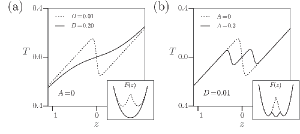
Figure 1: Force-elongation curves in the case of periodic driving (adiabatic limit). The equilibrium system ($A=0$) is shown in (a) and and out-of-equilibrium system ($A\neq 0$) - in (b). Here $k=0.6$.

Model. Consider the non-dimensional Langevin equation $\dot{x}=-\partial_{x}E+\sqrt{2D}\xi(t),$ where $\xi(t)$ is a standard delta correlated noise with zero average, $D$ is a measure of temperature and $E(x,z,t)=V(x)+k(x-z)^{2}/2-xf(t)$ is a time dependent potential. We assume that $V(x)=\left(|x|-1/2\right)^{2}/2$ is a bi-stable potential describing the conformational change and $z$ is a control parameter coupled through a spring of stiffness $k$ with the internal variable $x$. The energy is supplied to the system by a rocking force $f(t)$ characterized by an amplitude $A$ and a time scale $\tau$. The presence of a thermal noise in this mean field description suggests that the system has a finite size Paniconi and Oono (1997). The external force required to maintain the system in the steady regime is $T(z)=k[z-\overline{\langle x\rangle}],$ where $\overline{\langle x\rangle}=\underset{t\rightarrow\infty}{\lim}(1/t)\int_{0}^{t}\int_{-\infty}^{\infty}xp(x,t)dxdt$ is the double averaging over ensemble and time and $p(x,t)$ is the corresponding probability distribution.

The main object of our study is the effective potential $F(z)=\int^{z}T(s)ds$. While $z$ has been introduced as a constant parameter, it can be also viewed as a mesoscopic variable satisfying $\nu\dot{z}=-\partial_{z}E+f_{ext}+\sqrt{2\nu D}\xi(t)$ where the frictional timescale $\nu/k\gg\tau$ and $f_{ext}$ is a slowly varying external force. As we show in sup the dynamics of the ensemble and time averaged $z$ that we denote by $Z$ is governed by $\nu\dot{Z}=-\partial_{Z}F+\overline{f_{ext}}$. In the case of skeletal muscles, if $x$ characterizes the state of a generic cross bridge, $Z$ would be a measure of strain at the level of the whole half-sarcomere sup . Even in the absence of an explicit mesoscopic variables, the concept of an effective potential is useful for the study of the slow component of the motion Zaikin et al. (2000); *baltanas_experimental_2003; *landa_nonlinear_2013; *sarkar_controlling_2014.

Periodic driving. Suppose first that the driving is square shaped $f(t)=A(-1)^{n(t)}$ with $n(t)=\lfloor 2t/\tau\rfloor,$ where brackets denote the integer part. An analytically transparent case is when the correlation time $\tau$ is much larger than the escape time for the bi-stable potential $V$, e.g. Magnasco (1993). For $f(t)\equiv A$ we can find the stationary solution of the Fokker-Planck equation (with $z=const$) $\partial_{t}p=\partial_{x}\left[p\partial_{x}E+D\partial_{x}p\right]$ analytically, compute $\langle x(A)\rangle$ explicitly and then average the result over the period $\langle\langle x\rangle\rangle=[\langle x(A)\rangle+\langle x(-A)\rangle]/2$, see sup for details. The typical force-elongation curves $T(z)$ and the corresponding potentials $F(z)$, obtained in such adiabatic limit, are shown in Fig. 1. The equilibrium system with $A=0$ exhibits negative stiffness at $z=0$ where the effective potential $F(z)$ has a maximum (spinodal state). As temperature increases at $A=0$ we observe a standard entropic stabilization of the configuration $z=0$, see Fig. 1(a), which takes place as a second order phase transition at the equilibrium temperature $D_{e}=r/[8(1+k)]$ where $r$ is a root of a transcendental equation $1+\sqrt{r/\pi}\text{e}^{-1/r}/[1+\text{erf}(1/\sqrt{r})]=r/(2k)$ sup . As the degree of non-equilibrium, characterized by $A$, increases, the effective potential develops a pseudo-well with a minimum at $z=0$, see Fig. 1(b), and we associate this phenomenon with the emergence of active rigidity.

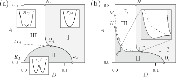
Figure 2: Phase diagram in ($A,D$) plane showing phases I,II and III: (a) - adiabatic limit, (b) - numerical solution at $\tau=100$ (b). $C_{A}$ is the tri-critical point, $D_{e}$ is the point of second order phase transion in a passive system. The Maxwell line for first order phase transition is shown by dots. Here $k=0.6$.

The non-equilibrium steady state (dynamic) phase diagram summarizing the results obtained in adiabatic approximation is shown in Fig. 2 (a). There, the ’paramagnetic’ phase I describes the regimes where the effective potential $F(z)$ is convex, the ’ferromagnetic’ phase II is a bi-stability domain where the potential $F(z)$ has a double well structure and, finally, phase III is where the function $F(z)$ has three convex branches separated by two concave (spinodal) regions. If we interpret the boundary $C_{A}-D_{e}$ separating phases I and II as a line of (zero force) second order phase transitions and the dashed line $C_{A}-M_{A}$ as a Maxwell line for the (zero force) first order phase transition, see sup , then $C_{A}$ will be a tri-critical point. Near this point the system can be described by the non-equilibrium Landau potential $F(z)=F_{0}+rz^{2}+qz^{4}+pz^{6}$ where the coefficients $r,q$ are the measures of passive and active excitations, respectively, while $p>0$ is a fixed parameter. Similar tri-critical point has been observed in the periodically driven mean field Suzuki-Kubo model of magnetism Tomé and de Oliveira (1990) which can be interpreted in our terms as a description of the $T=0$ behavior only.

The adiabatic approximation fails at low temperatures (small $D$) where the escape time diverges and in this domain the corrected phase diagram was obtained numerically by computing the appropriate periodic solutions of the Fokker-Plank equation, see Fig. 2 (b). The high temperature part of the diagram (tri-critical point, point $D_{e}$ and the vertical asymptote of the boundary separating phases I and III at large values of $A$ are captured adequately by the adiabatic approximation. The new feature is a dip of the boundary separating Phases II and III at some $D<D_{e}$ leading to an interesting re-entrant behavior (cf. Van den Broeck et al. (1994); Pilkiewicz and Eaves (2014)) which is an effect of stochastic resonance. To verify our numerics in the low temperature domain we used the Kramers approximation, to show that indeed $A=1/2$ at point $K$ and $A=1/2+k/4$ at point $M$, see sup .

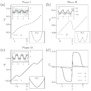
Figure 3: (a-c) Typical tension-length relations in phases I, II and III. Points $\alpha$, $\beta$ and $\gamma$ are the same as in Fig. 2 (b); (d) shows the active component of the force. Inserts illustrate the behavior of stochastic trajectories in each of the phases (gray lines) and their ensemble averages (black lines) at $z\simeq 0$. The other parameters: $k=0.6$, $\tau=100$.

Force-elongation relations in different points of the ($A,D$) phase diagram (Fig. 2 (b)) are shown in Fig. 3 where the insets illustrate the typical stochastic trajectories. We observe that while in phase I thermal fluctuations dominate periodic driving and undermine the two wells structure of the potential, in phase III the jumps between the two energy wells are fully synchronized with the rocking force. In phase II the system shows intermediate behavior with uncorrelated jumps between the wells. We conclude that the pseudo-well in phase III has a resonant nature and remark that somewhat similar phenomena were also observed in other driven out-of-equilibrium systems Cugliandolo et al. (2000); *munoz_generic_2005; *berthier_non-equilibrium_2013.

In Fig. 3(d) we show the active component of the force $T_{a}(z)=T(z;A)-T(z;0)$ representative of phases I, II and III. The active contribution is significant only in phase III and the corresponding plateau can be viewed as another signature of the presence of a pseudo-well. Interestingly, our prototypical device generates active tension of both signs which can be interpreted as pulling at $z>0$ and pushing at $z<0$. However, in the puling regime the linear spring is stretched while in the pushing regime it is compressed. Since in biological conditions the filaments responsible for passive stiffness would buckle in compression, e.g. Lenz et al. (2012), the pushing part of the active force-length relation is hardly realistic. On the other hand, the pulling part shows a striking resemblance to the isometric tetanus in skeletal muscles Gordon et al. (1966) that can be also driven through the bi-stable potential Sheshka and Truskinovsky (2014).

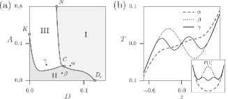
Figure 4: (a) Phase diagram in the case of DC driving. The identification of phases I, II,III is the same as in Fig. 2 (a,b). (b) Typical tension-length relations in different phases (b). Here $\tau=100$ and $k=0.6$.

In view of this analogy, detailed in sup , it is instructive to estimate the four non-dimensional parameters of the model by using the available data on molecular motors operating in muscle cells. We choose the time scale to be $\tau^{\star}=\eta/k_{0}\sim 0.1\text{ ms}$ where $\eta\sim 0.38\;\text{ms}.\;\text{pN}/\text{nm}$ is the viscosity adopted in Caruel et al. (2013) and $k_{0}\sim 3\;\text{pN}/\text{nm}$ is the stiffness of the cross-bridge in pre and post power stroke configurations. The spatial scale is $l^{\star}=a\sim 10\text{nm}$, the characteristic size of a motor power-stroke Linari et al. (2010) and the stress scale is $k^{\star}=k_{0}$. This leads to an energy scale $E^{\star}=k_{0}a^{2}\sim 200\;\text{pN}.\text{nm}$. Then, the non-dimensional parameters can be estimated as follows. Parameter $k=k_{m}/k^{\star}\sim 0.6$, where $k_{m}$ is the stiffness of the elastic part of the myosin motor Lewalle et al. (2008); Barclay et al. (2010). Temperature is $D=k_{B}\Theta/E^{\star}\sim 0.01$ where $k_{B}=4.10\text{ pN}.\text{nm}$ is the Boltzmann constant and $\Theta\sim 300\text{K}$ the ambient temperature. For the active driving time scale, we estimate $\tau=\tau_{a}/\tau^{\star}\sim 100$ where $\tau_{a}=40\text{ ms}$ is the characteristic time of ATP hydrolysis Howard (2001). Finally we take $A=\sqrt{\Delta\mu/E^{\star}}\approx 0.5$ where $\Delta\mu=20k_{B}\Theta$ is the degree of non-equilibrium of the hydrolysis reaction Howard (2001). The obtained estimate ($A=0.5,D=0.01$) suggests that muscle myosins, operating in stall conditions (isometric contractions), are in phase III. The proposed representation of the ATP hydrolysis (through parameter $A$) explains stabilization of the power stroke mechanism in skeletal muscles in the negative stiffness regime Caruel et al. (2013) and may be also behind titin based force generating mechanism at long sarcomere lengths that does not rely on actin-myosin based cross-bridge interactions Schappacher-Tilp et al. (2015).

Dichotomous driving. To ascertain the robustness of these results we now consider a different representation of the external forcing as a dichotomous (DC) or telegraphic noise, e.g. Ichiki et al. (2012); Nagai et al. (2015). In this case $f(t)=A(-1)^{n(t)},$ where $n(t)$ is a Poisson process with ($P(n)=e^{-\lambda}\lambda^{n}/n!$ and rate parameter $\lambda=1/(2\tau)$; we thus have $\left\langle f(t)\right\rangle=A\exp(-t/\tau)$ and $\left\langle f(t),f(s)\right\rangle=A^{2}\exp(-|t-s|/\tau).$ The DC driven system is controlled by the same number of parameters as the periodically driven system, however, the problem is no longer analytically tractable. The numerical solution of the ensuing stochastic differential equation shows that the qualitative structure of the phase diagram in the ($A,D$) plane remains the same as in the case of periodic driving, see Fig.4. We checked our numerical results by considering an analytically tractable double limit when $\tau\rightarrow 0$, $A\rightarrow\infty$, while $\tilde{D}=A^{2}\tau$ remains finite. In this limit phase III disappears because the system can be viewed as exposed to a white noise with effective temperature $D^{*}=\sqrt{D^{2}+\tilde{D}^{2}}$. Then there is only a second order phase transition at the expected value of the parameter $D^{*}_{e}=r/[8(1+k)]$. This simple limit highlights the crucial role of correlations in the noise ($\tau\neq 0$). Our next example, however, shows that correlations per se are not enough.

Ornstein-Uhlenbeck driving. Suppose now that $f(t)$ is a solution of a linear stochastic differential equation $\dot{f}=-f(t)/\tau+A\sqrt{2/\tau}\xi_{f}(t),$ where $\xi_{f}(t)$ is a standard white noise independent of $\xi(t)$. Such non-equilibrium driving is known as Ornstein-Uhlenbeck (OU) noise, e.g. Bartussek (1997); Nagai et al. (2015) , and its first ($\left\langle f(t)\right\rangle$) and second ($\left\langle f(s)f(t)\right\rangle$) moments are the same as in the case of DC if we assume, without loss of generality, that $f(0)=A$. The Fokker-Planck equation for the probability density $p(x,f,t)$ takes the form $\partial_{t}p=\partial_{x}(p\partial_{x}E+D\partial_{x}p)+\tau^{-1}\partial_{f}(fp+A^{2}\partial_{f}p).$ By solving it numerically we obtain a phase diagram shown in Fig. 5(a). A striking feature of this diagram is that phase III is missing because, in contrast to periodic and DC case, the noise is now unbounded and the system can always escape from a neighborhood of a resonant state. The behavior of the force-elongation relations shown in Fig. 5(b) is compatible with the idea of purely entropic stabilization, in particular, the limit of thermal noise is again recovered when $\tau\rightarrow 0$ and $A\rightarrow\infty$, with $\tilde{D}=A^{2}\tau$ fixed.

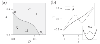
Figure 5: (a) Phase diagram in the case of OU driving. The identification of phases I, II is the same as in Fig. 2 (a,b). (b) The typical tension-length relations in different phases. Here $\tau=100$ and $k=0.6$.

Zero temperature limit. To clarify further the differences between our three representations of a non-equilibrium bath, we compare in all three cases the ($\tau,\tilde{D}$) phase diagrams corresponding to the limit $D\rightarrow 0$ where the thermal component of the noise is absent. In the DC case the solution of the limiting Fokker-Plank equation can be written explicitly Hänggi and Jung (1995)

$$p_{DC}(x)\sim Q(x)^{-1}\exp\left(-\int^{x}\frac{\partial_{y}\tilde{V}(y)/\tau}{A^{2}-(\partial_{y}\tilde{V}(y))^{2}}dy\right).$$

where $Q=A^{2}-(\partial_{x}\tilde{V}(x))^{2}$ and $\tilde{V}=V+k(x-z)^{2}/2$. The choice of the normalization constant depends on the parameters and is detailed in sup . The resulting phase diagram, shown in Fig. 6(a), exhibits all three phases with a tri-critical point $C^{\prime}$ located at $\tau_{C^{\prime}}=[2(k+1)]^{-1}$ and $\tilde{D}_{C^{\prime}}=D_{e}+[2(k+1)]^{-1}/4$. The behavior of the force-elongation relations in different phases is illustrated in Fig. 6(b).

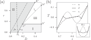
Figure 6: (a) Phase diagram in the case of DC driving. The identification of phases I, II and III is the same as in Fig. 2 (a,b). The dash-dotted line - the boundary between phases II and III (periodic driving); the dashed line - the boundary between Phases I and II (OU driving). (b) Typical tension-length relations in the case of DC driving in different phases (b). Parameters $k=0.6$, $D=0$.

In the case of OU driving with $D=0$ an analytical approximation of the stationary probability distribution is available for small $\tau$ only Hänggi and Jung (1995)

$$p_{OU}(x)\sim R(x)\exp\left(-\frac{\tilde{V}(x)+\tau(\partial_{x}\tilde{V}(x))^{2}/2}{A^{2}\tau}\right)$$

where $R(x)=|1+\tau\partial_{xx}\tilde{V}(x)|$, see sup for the details. The resulting phase diagram does not contain phase III and the line dividing phases I and II is shown in Fig. 6(a) (dashed line). The problem with periodic driving exhibits in the limit $D\rightarrow 0$ only phases II and III even for rapidly oscillating external fields, see the dash-dotted line in Fig. 6(a). In this perspective, the DC driving emerges as an intricate amalgam of OU and periodic noises with none of them dominating the other.

Conclusions. To complement the existing microscopic models of force generation (Brownian ratchets), we proposed a conceptually similar model of rigidity generation (Brownian snap-springs). The model, invoking some interesting parallels between condensed matter physics and biomechanics, shows that by controlling the degree of non-equilibrium in the system, one can modify the structure of the effective energy landscape. In particular, this implies that unstable or marginally stable mechanical states may be stabilized by out-of-equilibrium ATP hydrolysis reaction. Our results also suggest that the mechanical action of a non-equilibrium reservoir can be crucially sensitive to the higher moments of the stochastic noise.

The authors thank J.-F. Joanny, R. García García and M. Caruel for helpful discussions.

References

- Broedersz and MacKintosh (2014) C. P. Broedersz and F. C. MacKintosh, Rev. Mod. Phys. 86, 995 (2014).
- Koenderink et al. (2009) G. H. Koenderink, Z. Dogic, F. Nakamura, P. M. Bendix, F. C. MacKintosh, J. H. Hartwig, T. P. Stossel, and D. A. Weitz, PNAS 106, 15192 (2009).
- Ranft et al. (2010) J. Ranft, M. Basan, J. Elgeti, J.-F. Joanny, J. Prost, and F. Jülicher, PNAS 107, 20863 (2010).
- Martin et al. (2000) P. Martin, A. D. Mehta, and A. J. Hudspeth, PNAS 97, 12026 (2000).
- Batters et al. (2004) C. Batters, M. I. Wallace, L. M. Coluccio, and J. E. Molloy, Phil. Trans. R. Soc. Lond. B 359, 1895 (2004).
- Vilfan and Duke (2003) A. Vilfan and T. Duke, Biophys. J. 85, 818 (2003).
- Caruel et al. (2013) M. Caruel, J.-M. Allain, and L. Truskinovsky, Phys. Rev. Lett. 110, 248103 (2013).
- Schillers et al. (2010) H. Schillers, M. Wälte, K. Urbanova, and H. Oberleithner, Biophys. J. 99, 3639 (2010).
- Hawkins and Liverpool (2014) R. J. Hawkins and T. B. Liverpool, Phys. Rev. Lett. 113, 028102 (2014).
- Étienne et al. (2015) J. Étienne, J. Fouchard, D. Mitrossilis, N. Bufi, P. Durand-Smet, and A. Asnacios, PNAS , 201417113 (2015).
- Ingber et al. (2014) D. E. Ingber, N. Wang, and D. Stamenović, Rep. Prog. Phys. 77, 046603 (2014).
- Onck et al. (2005) P. R. Onck, T. Koeman, T. van Dillen, and E. van der Giessen, Phys. Rev. Lett. 95, 178102 (2005).
- Fletcher and Mullins (2010) D. A. Fletcher and R. D. Mullins, Nature 463, 485 (2010).
- Pritchard et al. (2014) R. H. Pritchard, Y. Y. S. Huang, and E. M. Terentjev, Soft Matter 10, 1864 (2014).
- Ronceray et al. (2015) P. Ronceray, C. Broedersz, and M. Lenz, arXiv:1507.05873 (2015).
- Kobirumaki-Shimozawa et al. (2014) F. Kobirumaki-Shimozawa, T. Inoue, S. A. Shintani, K. Oyama, T. Terui, S. Minamisawa, S. Ishiwata, and N. Fukuda, J. Physiol. Sci. 64, 221 (2014).
- Butikov (2011) E. I. Butikov, J. Phys. A: Math. Theor. 44, 295202 (2011).
- Vočadlo et al. (2003) L. Vočadlo, D. Alfè, M. J. Gillan, I. G. Wood, J. P. Brodholt, and G. D. Price, Nature 424, 536 (2003).
- Puglisi and Truskinovsky (2013) G. Puglisi and L. Truskinovsky, Phys. Rev. E 87, 032714 (2013).
- Fritzen and Kochmann (2014) F. Fritzen and D. M. Kochmann, Int. J. Solids Struct. 51, 4101 (2014).
- Bukov et al. (2015) M. Bukov, L. D’Alessio, and A. Polkovnikov, Adv. Phys. 64, 139 (2015).
- Sarkar et al. (2015) P. Sarkar, A. Shit, S. Chattopadhyay, and S. K. Banik, Chem. Phys. 458, 86 (2015).
- Caruel et al. (2015) M. Caruel, J. M. Allain, and L. Truskinovsky, J. Mech. Phys. Solids 76, 237 (2015).
- Reimann (2002) P. Reimann, Phys. Rep. 361, 57 (2002).
- Gallardo et al. (2012) R. Gallardo, O. Idigoras, P. Landeros, and A. Berger, Phys. Rev. E 86, 051101 (2012).
- Fogle et al. (2015) C. Fogle, J. Rudnick, and D. Jasnow, arXiv:1502.00343 [cond-mat] (2015).
- Paniconi and Oono (1997) M. Paniconi and Y. Oono, Phys. Rev. E 55, 176 (1997).
- (28) See Supplemental Material at [URL will be inserted by publisher].
- Zaikin et al. (2000) A. A. Zaikin, J. Kurths, and L. Schimansky-Geier, Phys. Rev. Lett. 85, 227 (2000).
- Baltanás et al. (2003) J. P. Baltanás, L. Lopez, I. I. Blechman, P. S. Landa, A. Zaikin, J. Kurths, and M. A. F. Sanjuán, Phys. Rev. E 67, 066119 (2003).
- Landa and McClintock (2013) P. S. Landa and P. V. E. McClintock, Phys. Rep. 532, 1 (2013).
- Sarkar et al. (2014) P. Sarkar, A. K. Maity, A. Shit, S. Chattopadhyay, J. R. Chaudhuri, and S. K. Banik, Chem. Phys. Lett. 602, 4 (2014).
- Magnasco (1993) M. O. Magnasco, Phys. Rev. Lett. 71, 1477 (1993).
- Tomé and de Oliveira (1990) T. Tomé and M. J. de Oliveira, Phys. Rev. A 41, 4251 (1990).
- Van den Broeck et al. (1994) C. Van den Broeck, J. M. R. Parrondo, and R. Toral, Phys. Rev. Lett. 73, 3395 (1994).
- Pilkiewicz and Eaves (2014) K. R. Pilkiewicz and J. D. Eaves, Soft Matter 10, 7495 (2014).
- Cugliandolo et al. (2000) L. F. Cugliandolo, D. R. Grempel, and C. A. da Silva Santos, Phys. Rev. Lett. 85, 2589 (2000).
- Muñoz et al. (2005) M. A. Muñoz, F. d. l. Santos, and M. M. T. d. Gama, Eur. Phys. J. B 43, 73 (2005).
- Berthier and Kurchan (2013) L. Berthier and J. Kurchan, Nat. Phys. 9, 310 (2013).
- Lenz et al. (2012) M. Lenz, T. Thoresen, M. L. Gardel, and A. R. Dinner, Phys. Rev. Lett. 108, 238107 (2012).
- Gordon et al. (1966) A. M. Gordon, A. F. Huxley, and F. J. Julian, J. Physiol. 184, 170 (1966).
- Sheshka and Truskinovsky (2014) R. Sheshka and L. Truskinovsky, Phys. Rev. E 89, 012708 (2014).
- Lewalle et al. (2008) A. Lewalle, W. Steffen, O. Stevenson, Z. Ouyang, and J. Sleep, Biophys. J. 94, 2160 (2008).
- Barclay et al. (2010) C. Barclay, R. Woledge, and N. Curtin, Prog. Biophys. Mol. Bio. 102, 53 (2010).
- Linari et al. (2010) M. Linari, M. Caremani, and V. Lombardi, Proc. Biol. Sci. 277, 19 (2010).
- Howard (2001) J. Howard, Mechanics of motor proteins and the cytoskeleton (Sinauer Associates Inc.-Publishers Sunderland, Massachusetts, 2001).
- Schappacher-Tilp et al. (2015) G. Schappacher-Tilp, T. Leonard, G. Desch, and W. Herzog, PloS one 10 (2015).
- Ichiki et al. (2012) A. Ichiki, Y. Tadokoro, and M. I. Dykman, Phys. Rev. E 85, 031106 (2012).
- Nagai et al. (2015) K. H. Nagai, Y. Sumino, R. Montagne, I. S. Aranson, and H. Chaté, Phys. Rev. Lett. 114, 168001 (2015).
- Bartussek (1997) R. Bartussek, in Stochastic Dynamics, Lecture Notes in Physics No. 484, edited by L. Schimansky-Geier and T. Pöschel (Springer Berlin Heidelberg, 1997) pp. 68–80.
- Hänggi and Jung (1995) P. Hänggi and P. Jung, in Advances in Chemical Physics, Vol. 89 (John Wiley & Sons Inc, 1995) pp. 239–326.