A test of the nature of the Fe K Line in the neutron star low-mass X-ray binary Serpens X-1

Abstract

Broad Fe K emission lines have been widely observed in the X-ray spectra of black hole systems, and in neutron star systems as well. The intrinsically narrow Fe K fluorescent line is generally believed to be part of the reflection spectrum originating in an illuminated accretion disk, and broadened by strong relativistic effects. However, the nature of the lines in neutron star LMXBs has been under debate. We therefore obtained the longest, high-resolution X-ray spectrum of a neutron star LMXB to date with a 300 ks Chandra HETGS observation of Serpens X-1. The observation was taken under the “continuous clocking” mode and thus free of photon pile-up effects. We carry out a systematic analysis and find that the blurred reflection model fits the Fe line of Serpens X-1 significantly better than a broad Gaussian component does, implying that the relativistic reflection scenario is much preferred. Chandra HETGS also provides highest spectral resolution view of the Fe K region and we find no strong evidence for additional narrow lines.

1. Introduction

Broad iron emission lines have been widely discovered in Active Galactic Nuclei (AGN; Tanaka et al. 1995; Fabian et al. 2009; Brenneman et al. 2011), and low-mass X-ray binaries (LMXBs) including stellar-mass black holes (Done & Zycki, 1999; Miller et al., 2002; Miller, 2007; Reis et al., 2009) and neutron stars (NS; Asai et al. 2000; Barret et al. 2000; Oosterbroek et al. 2001; Di Salvo et al. 2005; Bhattacharyya & Strohmayer 2007; Iaria et al. 2007; Cackett et al. 2008, 2009a, 2010; Sanna et al. 2013; Di Salvo et al. 2015; Pintore et al. 2015). An accretion disk is believed to orbit the central object, and a hard X-ray source, either a powerlaw continuum or a blackbody component (potentially the “boundary layer”), emits hard X-rays that illuminate the accretion disk. Atomic transitions take place after the high-energy photons are absorbed, resulting in a reflection spectrum including several narrow emission lines and a broad feature peaked around 20-30 keV which is known as “Compton hump” (Lightman & White, 1988; George & Fabian, 1991; Ross & Fabian, 1993; Matt et al., 1993; Ross & Fabian, 2005; García & Kallman, 2010a; Ballantyne et al., 2012).

The Fe K$\alpha$ fluorescent line is the most prominent feature in the reflection spectrum. When appearing in the X-ray spectra of AGN and LMXBs, the intrinsically narrow Fe lines sometimes show broad, asymmetric profiles which are generally believed to be shaped by a series of relativistic effects induced from strong gravitational fields (Fabian et al., 1989, 2000). As relativistic effects are stronger in the area closer to the compact object, the line profile is sensitive to the inner radius of the accretion disk. If the accretion disk extends to the innermost stable circular orbit (ISCO), one can, under certain assumptions, obtain an estimate of the black hole spin by measuring the inner radius of the accretion disk (Bardeen et al., 1972). The Fe K$\alpha$ line profile has been a powerful tool to measure black hole spin (e.g., Miller et al., 2002; Reynolds & Nowak, 2003; Brenneman & Reynolds, 2006; Miller, 2007; Reis et al., 2008, 2012). The inner radius of the accretion disk in a NS system can be determined by the same method. The accretion disk in a NS system could be truncated by the stellar surface or the boundary layer between the disk and the NS, if the NS is larger than its ISCO, or by a strong stellar magnetic field. An upper limit of the stellar radius of a NS can be given by measuring the inner radius of the disk, and hence help understand its equation of state (e.g. Piraino et al. 2000; Cackett et al. 2008). Bhattacharyya (2011) reported more detailed calculations to show how future instruments can directly constrain NS equation of state models using relativistic disk lines.

In NS systems, the Fe K$\alpha$ lines are usually not as prominent (EW $\sim$ 100 eV) as those seen in AGN and black hole binaries (BHBs) due to extra continuum emission from the boundary layer. It has been widely accepted that relativistic Fe K lines are common in AGN (Reynolds & Nowak, 2003) and BHBs (Miller, 2007), though some suggest line profiles to be caused by warm absorbers (Inoue & Matsumoto, 2003) or Comptonization (Laurent & Titarchuk, 2007). Nonetheless, whether Fe K lines in NS systems are relativistically broadened is still under debate. Ng et al. (2010) analyzed a number of XMM-Newton NS spectra and concluded that statistical evidence of asymmetric iron line profiles is lacking and the lines are broadened by Compton scattering in a disk corona (Misra & Kembhavi, 1998; Misra & Sutaria, 1999). Reynolds & Wilms (2000) showed that the continuum source required in the Compton scattering model to produce the broad iron line violates the blackbody limit. Although the calculation was based on the AGN case, small radii of the Compton clouds are still required to maintain the high ionization level in NS systems, which would make gravitational effects dominant (Fabian et al., 1995). Furthermore, the pile-up correction applied in Ng et al. (2010) reduced the signal-to-noise ratio of the data and made it difficult to detect relativistic iron lines (see Figure 2 in Miller et al. 2010). Cackett et al. (2010) examined a large sample of Suzaku NS spectra and found that the relativistic reflection scenario is much preferred. The iron line detections with Suzaku are less affected by photon pile-up effects than those of XMM-Newton, thus the conclusion that iron lines are asymmetric is likely more robust. A study of the effects of pile-up in X-ray CCD detectors by Miller et al. (2010) showed that while pile-up can distort the Fe K line profiles, it tends to artificially narrow them (in contrast with Ng et al. 2010).

Detections made with spectrometers that suffer no photon pile-up effects become important to determine the iron line profiles. The re-analyses of archival BeppoSAX data of 4U 1705-44 implied the existence of asymmetric Fe K lines (Piraino et al., 2007; Lin et al., 2010; Cackett et al., 2012; Egron et al., 2013). NuSTAR sees an asymmetric line in Serpens X-1 (Miller et al., 2013) with line properties consistent with Suzaku measurements from Cackett et al. (2008, 2010, 2012). The pile-up free detectors BeppoSAX and NuSTAR both reach the conclusion of relativistic iron lines. These instruments are, however, not capable of detecting possible narrow line components on top of the broad Fe K lines. Chandra HETGS is so far the only instrument that offers a pile-up free observation at high spectral resolution (approximate $\Delta$E$\sim$30 eV at 6 keV).

The neutron star LXMB Serpens X-1 was discovered in 1965 (Friedman et al., 1967). Being a persistent, bright X-ray source, Serpens X-1 has been observed with major X-ray missions, including Einstein (Vrtilek et al., 1986), ASCA (Asai et al., 2000), EXOSAT (Seon & Min, 2002), BeppoSAX (Oosterbroek et al., 2001), INTEGRAL (Masetti et al., 2004), XMM-Newton (Bhattacharyya & Strohmayer, 2007), Suzaku (Cackett et al., 2008, 2010) and recently with NuSTAR (Miller et al., 2013). It was also detected in optical (Hynes et al., 2004) and radio (Migliari et al., 2004) band. Relativistic Fe K lines have been reported several times in previous Suzaku, XMM-Newton and NuSTAR observations (Bhattacharyya & Strohmayer, 2007; Cackett et al., 2008, 2010; Miller et al., 2013). In this paper we study the latest high-resolution Chandra HETGS observation, which is the longest Chandra grating observation of a neutron star LMXB to date. We present detailed data analysis and results in the following sections. The Galactic absorption column $N_{\rm H}$ is assumed to be $4.4\times 10^{21}$ cm^-2(Dickey & Lockman, 1990) with “wilm” abundances (Wilms et al., 2000) throughout all our analyses, which were done using the XSPEC 12.8.2 package (Arnaud, 1996). All errors quoted in the paper are given at the 90 per cent confidence level.

2. Data Reduction

Serpens X-1 was observed with the Chandra High Energy Transmission Grating Spectrometer (HETGS) during 2014 June $27-29$ and 2014 August $25-26$ (Obs. ID: 16208, 16209), totaling a good exposure of $\sim$ 300 ks. The observation was taken using the “continuous clocking (CC)” mode. We reduced the data following the standard procedures using the latest CIAO V4.6 software package. The CC mode provides 2.85 ms time resolution, the observation is hence clear of photon pile-up effects and has negligible backgrounds. In this work we concentrate on the HEG (high energy grating) data which covers the Fe line energy band. We found the HEG +1 and $-1$ spectra to differ at the $5-10$% level, especially around the area of a chip gap in the +1 spectrum. Thus, we tested a number of methods to improve the +1 spectrum (see Appendix). However, the discrepancy cannot be completely eliminated, and thus we only use the HEG $-1$ spectrum in this work.

The spectra of each observation from June and August 2014 are similar and we combined them to form a long spectrum. All spectral bins from 2-8 keV have more than 30 counts per bin and thus no rebinning is required. We found a number of wiggles in the spectrum below 2 keV that could not be modeled. Their locations matched those where there are significant sharp changes in the effective area. We therefore use the $2.0-8.0$ keV energy band in the following analysis. A restricted energy band is often used for the data taken under the CC mode to avoid artificial instrumental artifacts (e.g., Cackett et al., 2009b; Miller et al., 2011, 2012; Degenaar et al., 2014).

The upper panel of Fig. 1 displays the $0.4-10.0$ keV light curves of Serpens X-1 during the observation. It can be seen that there is a weak type I X-ray burst, which originates from the thermonuclear burning of matter on the NS surfaces (Woosley & Taam, 1976; Lamb & Lamb, 1978; Strohmayer & Bildsten, 2006), in the later observation (shown in blue data points). The X-ray burst lasted for a few hundreds of seconds and contributed $\sim 4.7\times 10^{4}$ counts, which is only $\sim$ 0.5 per cent of the total $\sim 8.9\times 10^{6}$ counts of the entire observation. Since the burst is such a small fraction of the total counts and casts no effects on the spectrum, we did not exclude the data during the X-ray burst.

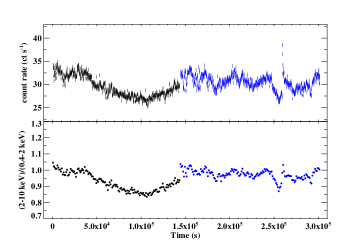
Figure 1.— The upper panel shows the 0.4-10 keV light curve of Serpens X-1. The light curve was extracted from the first order HEG data. The gap between the observations has been discarded. Black points stand for data extracted from the first half of the observation, and blue ones for the second. There is a weak type I X-ray burst containing $\sim$ 0.5 per cent of the total counts in the second half of the observation. The lower panel shows the hardness ratio, which is the hard (2-10 keV) light curve divided by the soft (0.4-2.0 keV) light curve.

Table 1Best-fitting parameters for different continuum models. Model 1a/1b includes both DISKBB and BBODY components; Model 2a/2b composes of DISKBB and the powerlaw continuum; Model 3a/3b comprises of BBODY and powerlaw components. Both Model 3a and Model 3b gave most reasonable fitting parameters.

Component	Parameter	Model 1a	Model 1b	Model 2a	Model 2b	Model 3a	Model 3b
TBABS	$N_{\rm H}$ ($10^{22}$ cm-2)	(0.44)	(0.44)	(0.44)	(0.44)	(0.44)	(0.44)
DISKBB	$kT_{\rm disk}$ (keV)	$1.34^{+0.05}_{-0.03}$	$1.42\pm 0.04$	$1.42\pm 0.01$	$1.44^{+0.01}_{-0.02}$	$\cdots$	$\cdots$
	$N_{\rm disk}$	$80.0^{+6.8}_{-8.3}$	$68.3^{+6.5}_{-3.4}$	$60.1^{+2.3}_{-3.0}$	$61.7^{+1.4}_{-2.8}$	$\cdots$	$\cdots$
BBODY	$kT_{\rm bb}$ (keV)	$2.39^{+0.33}_{-0.19}$	$2.90^{+0.82}_{-0.44}$	$\cdots$	$\cdots$	$0.90^{+0.20}_{-0.17}$	$0.90^{+0.02}_{-0.01}$
	$N_{\rm bb}$ ($10^{-2}$)	$2.6\pm 0.1$	$2.5^{+0.5}_{-0.2}$	$\cdots$	$\cdots$	$2.3\pm 0.1$	$2.4\pm 0.1$
POWERLAW	$\Gamma$	$\cdots$	$\cdots$	$0.94^{+0.28}_{-0.12}$	$0.68^{+0.29}_{-0.35}$	$1.78\pm 0.02$	$1.80\pm 0.02$
	$N_{\rm pow}$	$\cdots$	$\cdots$	$0.10\pm 0.04$	$0.05^{+0.05}_{-0.03}$	$0.88\pm 0.03$	$0.87^{+0.03}_{-0.02}$
GAUSSIAN	$E_{\rm line}$ (keV)	$6.62^{+0.04}_{-0.13}$	$6.48^{+0.09}_{-0.06}$	$6.52^{+0.05}_{-0.07}$	$6.43^{+0.05}_{-0.03}$	$6.43^{+0.05}_{-0.03}$	$6.40^{+0.02}$
	$\sigma$ (keV)	$0.26^{+0.15}_{-0.06}$	$0.61_{-0.11}$	$0.41_{-0.03}$	$0.61_{-0.03}$	$0.41_{-0.01}$	$0.61_{-0.02}$
	$N_{\rm gau}$ ($10^{-3}$)	$1.9^{+1.1}_{-0.5}$	$4.6^{+0.6}_{-1.4}$	$3.1^{+0.3}_{-0.4}$	$5.0\pm 0.6$	$3.1^{+0.3}_{-0.4}$	$5.3\pm 0.6$
	EW (eV)	$48^{+11}_{-10}$	$115^{+42}_{40}$	$76^{+20}_{-16}$	$123^{+75}_{-29}$	$74^{+16}_{-14}$	$128^{+41}_{-35}$
$\chi^{2}/d.o.f.$		2052/1852	2051/1852	2072/1852	2056/1852	2184/1852	2148/1852

3. Data Analysis

3.1. Continuum

Continuum models for NS LMXBs can be degenerate, at least over narrow wavelength ranges, as we have here. They can be equally well explained by different continuum models consisting of a disk blackbody, a blackbody-like component (to fit the boundary layer emission) and a powerlaw or Comptonized component (e.g., Barret 2001; Lin et al. 2007). We test three different continuum models, which are a disk blackbody plus a blackbody (Model 1), a disk blackbody plus a powerlaw (Model 2), and a blackbody plus a powerlaw (Model 3), in order to find out necessary spectral components required to interpret the spectrum of Serpens X-1 in this observation. As mentioned in section 2, we use the HEG $-1$ over the $2.0-8.0$ keV energy band. The Galactic absorption is modelled by TBABS in XSPEC, the accretion disk blackbody emission by DISKBB, and the thermal emission from the NS boundary layer by BBODY.

An iron emission line has been clearly detected in the HEG $-1$ spectrum, and we start by modeling the feature with a Gaussian line (GAUSSIAN in XSPEC). In all our fits, we restrict the line energy to be in the range of $6.4-6.97$ keV, where neutral/ionized iron K$\alpha$ lines can only appear. However, given the relatively narrow energy range of the continuum, we find that the width ($\sigma$) of the Gaussian tends to be large values (1 - 1.5 keV), and large normalizations giving equivalent widths (EWs) greater than 500 eV, even when fixing the energy of the line to 6.4, 6.7 or 6.97 keV. Since this is not seen in neutron star LMXB spectra, we restrict the width of the Gaussian based on previous fits to Serpens X-1. For instance, the broadest width that Ng et al. (2010) get when fitting a Gaussian to XMM data of Serpens X-1 is $\sigma=0.27^{+0.14}_{-0.11}$ keV. Fits to other archival spectra of Ser X-1 tend to give slightly broader Gaussians than this. For instance, averaging all the fits in Cackett et al. (2012) we find an average Gaussian width of $\sigma=0.61$ keV. Using these as a guide, we try spectral fits with (a) $\sigma$ restricted to be less than the upper limit of 0.41 keV from Ng et al., and (b) $\sigma$ restricted to be less than 0.61 keV from Cackett et al. (2012).

Including a broad Gaussian component in the iron line energy band significantly improves the fit (the smallest improvement was $\Delta\chi^{2}\sim 150$ lower with three fewer d.o.f), confirming the clear detection of the broad iron emission line (also see differences between model residuals in Fig. 2). In Table 1 we show the fitting results of the three possible continuum models. Note that we also tried fitting with all three continuum components, but found that the power-law index became unconstrained in those fits.

Models 1b & 2a-b give comparable quality fits, however, all result in unphysical parameters. In Model 1b, when a larger $\sigma$ is allowed than Model 1a, we get an unusually high blackbody temperature (see Table 1). Furthermore, when replacing the Gaussian with a DISKLINE, we get an unphysical blackbody temperature ($>5$ keV), which is insensitive to the data (the peak of the blackbody is well outside of the HEG energy range). A typical blackbody temperature seen in NS systems is generally below $\sim$ 2.5 keV(Lin et al., 2010, 2012; Piraino et al., 2012; Di Salvo et al., 2015). In Model 2a-b the photon indices for the power-law are very hard ($\Gamma=0.94$), which is also unexpected as photon indices of NS usually fall into the 1.5-3.0 range (Cackett et al., 2010, 2012; Egron et al., 2013; Di Salvo et al., 2015). Therefore, while Model 3a-b do not give the best fit statistically, we use that model for the continuum in the following analysis.

It is interesting to note that both models 1a and 1b fit equally well, yet have quite different Gaussian widths. This can be viewed as evidence that the broad line is asymmetric, since a relativistic line with a narrow core and broad red wing can be well fit by two Gaussians - one reasonably narrow and one broad (Cackett et al., 2008, 2012). Fits with two Gaussians to Suzaku spectra of Ser X-1 yield widths of 0.14 keV and 0.64 keV (Cackett et al., 2012), comparable to the widths in models 1a and 1b.

3.2. Iron Line

An iron emission line was clearly detected in the spectrum, implying that a reflection component is present in the system. The iron line of Serpens X-1 seems to extend for at least 1 keV, indicating possible signatures of relativistic effects similar to those seen in stellar-mass black holes and AGN. We test the nature of the line by fitting several different models. If the line is broadened by relativistic effects, it should be better fitted by a relativistic line model rather than a broad Gaussian. Given the high spectral resolution of the Chandra HEG, we also have the opportunity to test whether there are any narrow line components that contribute to the line shape that are otherwise unresolved with other detectors.

First, we tested the relativistic reflection model by fitting the Fe emission line using the DISKLINE (Fabian et al., 1989) model in XSPEC. We replaced the broad Gaussian component in Model 3a/3b with DISKLINE to build a new model (hereafter Model 4a). See Table 2 for best-fitting values. This model fits significantly better than a broad Gaussian, with an improvement of $\Delta\chi^{2}=133$ for two more degrees of freedom. We find an inner disk radius of $7.7\pm 0.1~{}R_{\rm G}$ (where $R_{\rm G}=GM/c^{2}$), and an inclination of $24\pm 1$ degrees. We show the iron line profile and the best-fitting DISKLINE model in Fig. 3. The DISKLINE component clearly fits the Fe line very well. Other relativistic line models such as LAOR and RELLINE were also tested, and all of them fit the Fe line as well as DISKLINE does, with similar parameters. Note that if we use Model 1a/1b for the continuum instead of Model 3a/3b, we get consistent DISKLINE parameters, and a large improvement in $\chi^{2}$ ($\Delta\chi^{2}\sim 72-73$), though because of the narrow energy range we get a high blackbody temperature which is unconstrained.

Table 2Best-fitting spectral parameters, testing different models for the Fe K emission line. Model 4a tests a relativistic line, while models 4b tests narrow lines only and 4c tests a combination of a broad Gaussian and narrow lines. The relativistic line model is by far the best fit. Note that the definition of emissivity index $\beta$ in the DISKLINE model is $\epsilon(r)=r^{\beta}$ (where $r$ is the disk radius) instead of $\epsilon(r)=r^{-q}$, and here we quote $q$, which is equal to $-\beta$.

Component	Parameter	Model 3b	Model 4a	Model 4b	Model 4c
TBABS	$N_{\rm H}$ ($10^{22}$ cm-2)	(0.44)	(0.44)	(0.44)	(0.44)
BBODY	$kT_{\rm bb}$ (keV)	$0.90^{+0.02}_{-0.01}$	$0.89^{+0.01}_{-0.02}$	$0.89\pm 0.01$	$0.90\pm 0.01$
	$N_{\rm bb}$ ($10^{-2}$)	$2.4\pm 0.1$	$2.4\pm 0.1$	$2.2\pm 0.1$	$2.3\pm 0.1$
POWERLAW	$\Gamma$	$1.80\pm 0.02$	$1.74\pm 0.02$	$1.75\pm 0.02$	$1.78\pm 0.01$
	$N_{\rm pow}$	$0.87^{+0.03}_{-0.02}$	$0.81^{+0.03}_{-0.02}$	$0.88^{+0.02}_{-0.03}$	$0.88\pm 0.01$
GAUSS 1 (broad)	$E_{\rm line1}$	$6.40^{+0.02}$	$\cdots$	$\cdots$	$6.4^{+0.03}$
	$\sigma$ (keV)	$0.61_{-0.02}$	$\cdots$	$\cdots$	$0.41_{-0.01}$
	$N_{\rm gau}$ ($10^{-3}$)	$5.3\pm 0.6$	$\cdots$	$\cdots$	$2.7\pm 0.3$
	EW (eV)	$128^{+41}_{-35}$	$\cdots$	$\cdots$	$64^{+16}_{-14}$
GAUSS 2 (width=0)	$E_{\rm line2}$	$\cdots$	$\cdots$	$6.57\pm 0.01$	$6.57\pm 0.01$
	$N_{\rm gau}$ ($10^{-4}$)	$\cdots$	$\cdots$	$2.1^{+0.6}_{-0.4}$	$1.4\pm 0.5$
	EW (eV)	$\cdots$	$\cdots$	$5^{+2}_{-1}$	$3^{+2}_{-1}$
GAUSS 3 (width=0)	$E_{\rm line3}$	$\cdots$	$\cdots$	$6.67\pm 0.01$	$6.67\pm 0.01$
	$N_{\rm gau}$ ($10^{-4}$)	$\cdots$	$\cdots$	$1.8^{+0.5}_{-0.4}$	$1.2\pm 0.5$
	EW (eV)	$\cdots$	$\cdots$	$5^{+1}_{-2}$	$3\pm 1$
DISKLINE	$E_{\rm line}$ (keV)	$\cdots$	$6.97_{-0.02}$	$\cdots$	$\cdots$
	$q$	$\cdots$	$5.65^{+0.51}_{-0.43}$	$\cdots$	$\cdots$
	$R_{\rm in}$ ($RM/c^{2}$)	$\cdots$	$7.7\pm 0.1$	$\cdots$	$\cdots$
	inclination	$\cdots$	$24\pm 1$	$\cdots$	$\cdots$
	$N_{\rm diskline}$ ($10^{-3}$)	$\cdots$	$5.8\pm 0.5$	$\cdots$	$\cdots$
	$EW$ (eV)	$\cdots$	$149\pm 15$	$\cdots$	$\cdots$
$\chi^{2}/d.o.f.$		2148/1852	2015/1850	2286/1851	2149/1848

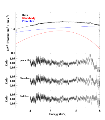
Figure 2.— The top panel shows the unfolded spectrum of Serpens X-1 with decomposed model components. We display the data/model ratios of the continuum model tbabs*(bbody + powerlaw), Model 3 and Model 3a in lower panels.

Next, we tested if the line could be fitted by two narrow Gaussian components (Model 4b). The line width $\sigma$ of each narrow Gaussian component was set to be zero. Model 4b gives a significantly worse fit than Model 3b, indicating that narrow lines alone cannot fit the data. We next tested for the presence of narrow lines in addition to a broad component (Model 4c), which gave a comparable fit than Model 3b, but a significantly worse fit than the relativistic line ($\Delta\chi^{2}=134$ higher, with two fewer d.o.f.). A model including three narrow lines was tested but did not improve the fit. We also tried to set the line energies of the narrow Gaussian components to be those of the Fe XXV (6.67 keV) and Fe XXVI (6.97 keV) lines, and again this did not yield a better fit. The equivalent widths of the narrow Gaussian lines in Model 4b and 4c are all small (EW $\sim 3-5$ eV). We also tested using narrow Gaussian components with physical upper limits of the line widths as well. Assuming a narrow line originates from outer part of the accretion disk and is broadened by thermal effects in a $\sim 10^{7}$ K gas, the line width should be $\sigma\lesssim 0.007$ keV. This again made no improvement in the fit. From the series of tests, we conclude that there is no strong evidence of narrow emission lines. We present detailed 6.0-7.0 keV data/model ratio in the lower panel of Fig. 4. It can be clearly seen that Model 4a fits this band very well and no obvious emission or absorption features are present.

In conclusion, of all the models we tried to fit the Fe K line in Serpens X-1, we find that a relativistic line model fits significantly better than any others, which indicates that the Fe line profile is caused by relativistic broadening and no narrow line components are required to explain the spectrum. The result acts to validate the relativistic reflection scenario.

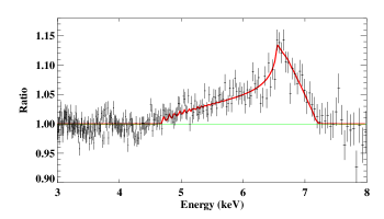
Figure 3.— The figure shows the Fe line profile of Serpens X-1. The spectrum is modeled as tbabs(bbody + powerlaw + diskline), and the plot is produced by setting the normalization of DISKLINE to be 0. The plot is visually binned with “septplot rebin” in XSPEC. The bin sizes through the Fe line are $\sim$ 0.042 keV. The red line shows model. It can been seen that the DISKLINE model fits the asymmetric line very well.

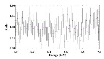
Figure 4.— The figure shows the 6.0-7.0 keV data/model ratio fitted using the DISKLINE model. The data are unbinned with bin sizes of $\sim$ 0.008 keV. It can be seen that no obvious emission or absorption features presenting in the figure.

3.3. Relativistic Reflection Model

As the Fe emission line is best interpreted by the relativistic reflection scenario, we replace the DISKLINE component in Model 4a with a blurred broadband reflection model. The reflection model self-consistently accounts for not only the Fe K line, but other lines and continuum emission expected due reflection, and broadening due to Comptonization based on the ionization parameter. The reflection model is then blurred by relativistic effects.

In NS systems, the accretion disk may be illuminated by the thermal emission coming from the boundary layer of the NS or by a power-law continuum, resulting in reflected emission (Cackett et al., 2010; D’Aì et al., 2010). The continuum of Serpens X-1 in this observation is dominated by the power-law component, and we use the REFLIONX model (Ross & Fabian, 2005), which calculates the broadband reflection spectrum from the accretion disk illuminated by a power-law continuum. The convolution model we use to account for relativistic effects is the KDBLUR kernel. We assumed the outer radius to be 400 $R_{\rm G}$. The iron abundance $A_{\rm Fe}$ was set to vary in the range between 1 and 4 times of solar value. The model fits the spectrum well, and we report the best-fitting parameters in Table 3. The values of the inner radius $R_{\rm in}$ and inclination angle $i$ we obtained are very similar to those given by Model 4a. The model using REFLIONX yielded a better fit than Model 4a ($\Delta\chi^{2}\sim 50$ lower with one fewer d.o.f.).

We also tested the XILLVER reflection model (García & Kallman, 2010b; García et al., 2013). While the fit using XILLVER yielded a worse fit than that using the REFLIONX grid, but the best-fitting parameters are comparable to that of Model 4a. In Table 3 it can be seen that models using different reflection grids gave consistent results. Parameters of KDBLUR obtained from both models are fairly similar, and both gave a inner radius of $R_{\rm in}\sim 7-8R_{\rm G}$ and a low inclination angle ($i\sim 30$).

Table 3The table lists fitting results of the relativistic reflection models. It can be seen that REFLIONX and XILLVER yield similar parameters.

Component	Parameter	REFLIONX	XILLVER
TBABS	$N_{\rm H}$	(0.44)	(0.44)
BBODY	$kT_{\rm bb}$ (keV)	$0.86\pm 0.01$	$0.87\pm 0.01$
	$N_{\rm bb}$ ($10^{-2}$)	$2.7\pm 0.1$	$2.6\pm 0.1$
POWERLAW	$\Gamma$	$1.68\pm 0.03$	$1.75\pm 0.03$
	$N_{\rm pow}$	$0.56\pm 0.06$	$0.73^{+0.02}_{-0.04}$
KDBLUR	$q$	$5.1^{+1.8}_{-1.0}$	$4.4^{+1.1}_{-0.7}$
	$R_{\rm in}$ ($R_{\rm G}$)	$7.1^{+1.1}_{-0.6}$	$8.4^{+1.1}_{-0.2}$
	$i$ (deg)	$29\pm 1$	$33\pm 1$
REFLECTION	$A_{\rm Fe}$	$1.00^{+0.56}_{-0.11}$	$1.52^{+1.47}_{-0.60}$
	$\xi$	$270^{+80}_{-30}$	$130^{+70}_{-30}$
	$N_{\rm ref}$	$6.8^{+2.0}_{-2.3}\times 10^{-5}$	$0.19^{+0.64}_{-0.15}$
$\chi^{2}/d.o.f.$		1968/1849	2012/1848

4. Discussion

We analyzed a 300 ks Chandra/HEG observation of the NS LMXB Serpens X-1. We fit a number of models to the $2-8$ keV HEG $-1$ spectrum to examine the nature of the Fe emission line, and find that the origin of the line is best explained by relativistically broadened reflection. Fitting broadband reflection models implies an inner radius of $\sim 7-8$ $R_{\rm G}$ and a low inclination of $i\sim 25^{\circ}-35^{\circ}$. In the following we discuss the robustness of the line parameters and compare our results with previous literature.

4.1. Choice of continuum model

It is difficult to constrain the continuum using a restricted $2-8$ keV energy band, and we choose the model with most reasonable fitting parameters (a blackbody and a powerlaw) to be the continuum in this work. In fact, Serpens X-1 has only been observed in the soft state, and the powerlaw component is usually weak. To explain the spectrum of a NS in the soft state, a continuum composed of a disk blackbody component contributed by the accretion disk and a blackbody component possibly caused by the thermal emission from the boundary layer (Model 1a/1b) is more likely. If replacing the Gaussian component with the DISKLINE model in Model 1a/1b and re-fitting the spectrum, we still obtain DISKLINE parameters similar to those of Model 4a ($E_{\rm line}=6.93\pm 0.04$ keV; emissivity index = $-5.2^{+0.5}_{-0.3}$; $R_{\rm in}=7.2\pm 0.1$ $R_{\rm G}$; $i=26\pm 1^{\circ}$). We also conduct the same test on Model 2a/2b, and find that the choice of continuum does not affect the parameters of the DISKLINE component.

Assuming the continuum of Serpens X-1 is soft and dominated by the thermal emission from the boundary layer, the illuminating source is then the blackbody component. In order to further test the broadband relativistic reflection model with a soft continuum (disk blackbody plus blackbody), we use the BBREFL grid (Ballantyne 2004; reflection calculated assuming a blackbody component to illuminate the accretion disk) instead of REFLIONX to account for reflection. The model composed of a soft continuum and relativistic reflection (KDBLUR*BBREFL) gives the best-fitting inner radius $R_{\rm in}=8.1^{+0.7}_{-1.2}$ $R_{\rm G}$ and inclination angle $i=34^{+1}_{-3}$^∘, which are consistent with those obtained using a harder continuum with the REFLIONX/XILLVER grids.

4.2. No additional narrow line components

In section 3.2 we test various models to fit the Fe K line and show that the line can simply be fitted by a relativistically broadened reflection component. Given the unique spectral resolution of Chandra HETGS, we have an opportunity to test for the presence of any narrow lines, in addition to the broad line. We find that including narrow lines in addition to a broad Gaussian gives a worse fit than the relativistic line alone. We include narrow Gaussian components with reasonable line energies (6.4 keV, 6.67 keV and 6.97 keV) to Model 4a and the broadband relativistic reflection models to examine the existence of narrow lines. Narrow components at 6.4 keV and 6.67 keV do not improve the fit of Model 4a, and the narrow Gaussian line at 6.97 keV improves the fit marginally ($\Delta\chi^{2}\sim 3$ lower than Model 4a). The narrow lines at 6.67 keV and 6.97 keV improve the fit of the REFLIONX model marginally ($\Delta\chi^{2}\sim 5-10$ lower than the REFLIONX model), but equivalent widths of these lines are low (EW $\sim 2$ eV). Furthermore, examination of Figure 4 shows no evidence for narrow lines in the residuals of the relativistic line fit. Hence, we conclude that there is no strong evidence of narrow components.

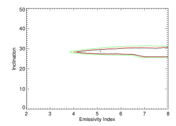
Figure 5.— The figure shows the contour plot of the emissivity index against the inclination angle, which was calculated from the REFLIONX model. The contours are plotted at 67% (black), 90% (red) and 99% (green) confidence levels. It can be seen that there is no claer degeneracy between emissivity and inclination angle.

4.3. Comparison with Previous Work

Bhattacharyya & Strohmayer (2007), Cackett et al. (2010) and Miller et al. (2013) reported the existence of relativistic Fe K lines in Serpens X-1 using XMM-Newton, Suzaku and NuSTAR data, respectively. In Bhattacharyya & Strohmayer (2007) the continuum was modeled as an absorbed Comptonization (compTT) plus a disk blackbody, while in the later two pieces of work a full continuum (a disk blackbody, a blackbody plus a powerlaw) was used. Bhattacharyya & Strohmayer (2007) used the LAOR model to fit the Fe K line, while Cackett et al. (2010) and Miller et al. (2013) used the blurred BBREFL and REFLIONX models to account for relativistic reflection. Bhattacharyya & Strohmayer (2007) obtained a inclination angle of $i\sim 40^{\circ}-50^{\circ}$, which is higher than the best-fitting values of Cackett et al. (2010) ($i\lesssim 25^{\circ}$) and Miller et al. (2013) ($i\lesssim 20^{\circ}$) and this work ($i\sim 30^{\circ}$). Cackett et al. (2010) also analyzed the same XMM-Newton data set used in Bhattacharyya & Strohmayer (2007) and found that low inclination ($i\lesssim 30^{\circ}$) is preferred.

Cackett et al. (2010) and Miller et al. (2013) both obtained a low emissivity index of $q\sim 2.3$, while a higher value of $q\sim 4-5$ is required in this work. We note that inclination and emissivity can be degenerate (see Fig. 8 in Cackett et al., 2010), but the degeneracy was not found in this work (see Fig. 5). The emissivity index depends on the Fe K line profile, and it is likely that the line profile is slightly different from those of previous observations because the better spectral resolution of Chandra grating data in this energy band. Regardless, our fits suggest a small inner radius, consistent with previous findings. In this work, the broad iron line profile implies an inner radius of $\sim 7-8$ $R_{\rm G}$. Previous analyses on XMM-Newton, Suzaku and NuSTAR data suggest the inner radius to be $\sim 4-25$ $R_{\rm G}$, $\sim 6-8$ $R_{\rm G}$, and $\sim 6-8.5$ $R_{\rm G}$, respectively. The XMM-Newton observation was taken under timing mode with a short exposure time, which causes some uncertainties in constraining parameters. The later Suzaku, NuSTAR and current observations all give well-constrained, consistent measurements of the inner radius. Although different continuum models were used to fit the spectra of Serpens X-1 observed with various instruments at different times/fluxes, previous and current analyses all indicate the source to have low inclination angle and small inner radius.

All previous observations of Serpens X-1 discussed above place the inner disk radius close to the ISCO. When comparing to the broader class of NS LMXBs, most other sources have an inner disk radius consistent with the ISCO, regardless of source luminosity (for instance see Figure 7 of Cackett et al., 2010, for a comparison over two orders of magnitude in luminosity). Clear exceptions to this are SAX J1808.4$-$3658 (Cackett et al., 2009a; Papitto et al., 2009), IGR J170480$-$2446 (Miller et al., 2011), and GRO J1744$-$28 (Degenaar et al., 2014), all of which are pulsars whose magnetic field must truncate the inner accretion flow. In low/hard states, accretion flow models suggest that the disk should recess, being replaced by a hot radiatively inefficient flow (see e.g., Done et al., 2007, for a review). However, iron line studies of NS LXMBs in low states do not show large disk truncation. For instance, a NuSTAR observation of 4U 1608-52 at 1-2 per cent of the Eddington limit has a disk that extends close to the ISCO (Degenaar et al., 2015), while broadband Suzaku observations of 4U 1705$-$44 at 3 per cent Eddington also shows the disk is not truncated at large radii (Di Salvo et al., 2015). Thus, the majority of NS LMXBs, including Serpens X-1, show inner disk radii that are close to the ISCO, with no strong dependence on state or luminosity.

5. Conclusion

We analyze the latest long HETGS data of Serpens X-1 and examine the nature of its Fe emission line. A thermal blackbody component possibly contributed by the boundary layer of the NS, and a power-law component provides a good fit to the continuum without unphysical parameters. By studying the Fe emission line in the spectrum, we find that the relativistic reflection scenario is much preferred, which is consistent with previous studies. Cackett et al. (2010) analyzed Suzaku data of Serpens X-1 and found relativistically-blurred iron emission lines. The recent NuSTAR observation (Miller et al., 2013) confirms the presence of the relativistic iron line, together with the Compton hump. In this work, we construct several models to test the relativistic reflection scenario and find that blurred reflection explains the Fe line profile significantly better than single/multiple Gaussian lines. Thanks to the remarkable resolving power of Chandra HETGS, the grating spectrum is capable of detecting narrow emission lines. In our analysis, no narrow line components are required, and must be weak if existent.

The broad iron line profile implies a small inner radius, and we obtain an inner radius of $\sim 7-8R_{\rm G}$. This sets an upper limit to the NS radius of $\sim 15-17$ km (assuming the mass of the NS is $\sim$ 1.4 $M_{\odot}$). Furthermore, a low inclination angle of $\sim 25-35$ degrees is found, which is consistent with the previous measurements. We also find that the choice of continuum does not affect the values of the line-related parameters, which further confirms the robustness of the fitting results. We conclude that the Fe emission line observed in the X-ray spectrum of Serpens X-1 is broad and shaped by relativistic effects.

Appendix A Discrepancy between the +1 and $-1$ Spectra

We aim at analyzing data with the maximum signal-to-noise ratio, so seek to combine the HEG +1 and $-1$ spectra. The HEG $\pm 1$ spectra are, however, discrepant and not suitable for combination. In Fig. 6 we plot the detector effective areas and data/model ratio of the HEG $\pm 1$ spectra (+1 in black and $-1$ in red data points) fitted by a simple continuum tbabs*(diskbb + bbody + powerlaw). It can been seen that the $\pm 1$ spectra disagree in most of the HEG energy band (at the $5-10$% level), though both show similar Fe line profiles when the continuum is properly modeled. The wiggles and emission features shown in the $-1$ spectrum below 2.0 keV cannot be modeled and match changes in the effective area, thus are likely due to calibration uncertainties. There are obvious deviations over the $2-5$ keV band between the $\pm 1$ spectra. It seems the HEG +1 spectrum suffers calibration problems, while the HEG $-1$ spectrum does not show unexpected features in the $2-5$ keV energy band. The location of the zeroth order image on the chip determines at which energies the chip gaps lie. Here, a 1 arcmin y-offset was applied on the zeroth order in order to place it in a location to avoid any chip gaps near the Fe K band. This results in a chip gap at around 2.5 keV in the +1 spectrum. Use of such an offset is not widely reported previously, which may explain the issues here. The $\sim$2.5 keV drop in the +1 spectrum matches with a large change in the effective area due to a chip gap (as marked by dashed lines in Fig. 6). Uncertain calibration around this gap clearly leads to the residuals. There also seems to be excess emission around the $3-4$ keV. This has been a known issue for HETGS data in CC mode, probably causing by improper order sorting table (OSIP) or charge transfer inefficiency (CTI) corrections¹.

Different from the “time event (TE)” mode, in CC mode every CCD suffers from time-dependent CTI. The CTI correction relies on charge trap maps for each device to predict charge losses and correct them. Nevertheless, in CC mode charges are clocked continuously and possibly leads to time-dependent charge trap maps, and each CCD suffers from this effect. Inappropriate CTI correction may cause events to fall out of the OSIP. So far, alternate trap maps for CC mode are not found, but the Chandra calibration team provided a few possible methods to solve this issue. One can primarily use HEG $-1$ and MEG +1 orders only, or apply a custom OSIP to possibly fix the problem.

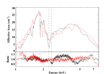
Figure 6.— We plot the HEG +1 (in black) and $-1$ (in red) detector effective areas in the upper panel. The lower panel of the figure shows the Serpens X-1 HEG +1 (black data points) and $-1$ (red data points) data/model ratios. The continuum is modeled as tbabs*(diskbb + bbody + powerlaw). The plot reveals the poor calibration of the HEG +1 spectrum. The vertical dashed lines are intended to help guide the eye.

We examined the order-sorting regions of each CCD by plotting the grating wavelength (wavelength times order) against the wavelength over the CCD wavelength ($hc$/ENERGY). Only HEG first order data have been used, and we show the order-sorting regions of chips S2 and S3, where the $\sim$ $2-5$ keV $\pm 1$ spectra were extracted from, in Fig. 7. Ideally data points should be evenly distributed along the $y=1$ axis. Most events on chip S2 lie slightly above unity (and so as those on S1, S4 and S5), while the distribution of those on chip S3 shows mild curvatures, which might be the reason that the +1 spectrum is not consistent with the $-1$ spectrum. One possible way to improve the $\pm 1$ spectral agreement is to modify the event file and bring the $y$-value in Fig. 7 close to unity. We first tried to correct the ENERGY column in the level=1.5 (after order-sorting) event file by dividing the column by the average $y$-value of each chip, and extract spectra from the corrected event file. We also tried a more sophisticated method, which is modifying the ENERGY column node by node, i.e., applying a spline fit to make every event lies on $y=1$. However, neither of the methods made the spectra noticeably better. We then tried to modify the level=1 (before order-sorting) event file and re-run tg_resolve_events to process order-sorting on the corrected event file, and extracted a new spectrum from the new event file after order-sorting. Modifying the level=1 event file does give different spectra, but it seems it causes problems to order-sorting and the spectra are clearly not corrected properly.

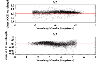
Figure 7.— The order-sorting region of chips S2 and S3. The x-axis is the wavelength times order, and the y-axis the absolute value of x-value over the CCD wavelength. The figure shows the selected events during the order-sorting process. The mild curvature shown in S3 might be the cause of discrepancy between the HEG $\pm 1$ spectra.

Another method to tackle this issue is to widen the order-sorting window. When data are taken under the CC mode, the Y position of an event is not known, and the order selection can be tricky. In some cases the spectra can be smoothed out by including events fell out of the OSIP. When running tg_resolve_events, by setting the script to disable the original OSIP file and indicating numbers of parameters “osort_hi” and “osort_lo”, one can customize the size of the order-sorting window. We set both osort_hi and osort_lo to be 0.2 (including events fell in the regime $0.8<y<1.2$ in Fig. 7) to widen the event order-sorting window. We find that this does not help eliminate discrepancies between the $\pm 1$ spectra, but on the contrary, makes the issue worse. By widening the order-sorting window, more events are selected and hence spectra with higher fluxes are created. The 3-4 keV excess emission in the +1 spectrum turned to be larger than the original spectrum before correction. In this case, widening the order-sorting window does not effectively solve the problem.

We look for a correction that would remove the 3-4 keV excess from the HEG +1 spectrum. As widening the order-sorting would increase the flux of this energy band, narrowing the window might give a correction that we need. We find that setting osort_hi=0.2 and osort_lo=0.04 (including events fell in the regime $0.96<y<1.2$) improves the agreement of the $\pm 1$ spectra. The corrected +1 spectrum does not completely match the $-1$ spectrum, but the flux level between $2-5$ keV is much more similar than the spectrum before correction. Although unfortunately it is still not good enough to combine the $\pm 1$ spectra and achieve maximum signal-to-noise ratio, we find that applying a SMEDGE component in XSPEC with negative optical depth to the +1 spectrum when fitting significantly improves data agreement over the $2-5$ keV energy band. The SMEDGE component can mimic the sharp feature caused by the change in effective area and reduce the residuals. Yet it seems that different continuum models are required to fit the +1 and $-1$ spectra, thus we only present results of the $-1$ spectrum in the paper. Nevertheless, fitting the +1 spectrum including the SMEDGE and allowing for a different continuum model than the $-1$ spectrum, results in the same conclusions and consistent parameters for the relativistic iron line.

References

- Arnaud (1996) Arnaud, K. A. 1996, in Astronomical Society of the Pacific Conference Series, Vol. 101, Astronomical Data Analysis Software and Systems V, ed. G. H. Jacoby & J. Barnes, 17
- Asai et al. (2000) Asai, K., Dotani, T., Nagase, F., & Mitsuda, K. 2000, ApJS, 131, 571
- Ballantyne (2004) Ballantyne, D. R. 2004, MNRAS, 351, 57
- Ballantyne et al. (2012) Ballantyne, D. R., Purvis, J. D., Strausbaugh, R. G., & Hickox, R. C. 2012, ApJ, 747, L35
- Bardeen et al. (1972) Bardeen, J. M., Press, W. H., & Teukolsky, S. A. 1972, ApJ, 178, 347
- Barret (2001) Barret, D. 2001, Advances in Space Research, 28, 307
- Barret et al. (2000) Barret, D., Olive, J. F., Boirin, L., et al. 2000, ApJ, 533, 329
- Bhattacharyya (2011) Bhattacharyya, S. 2011, MNRAS, 415, 3247