Causal Space-Times on a Null Lattice

Martin Schaden Department of Physics, Rutgers University, 101 Warren Street, Newark NJ 07102
Abstract

I investigate a discrete model of quantum gravity on a causal null-lattice with $SL(2,\mathbb{C})\,$structure group. The description is geometric and foliates in a causal and physically transparent manner. The general observables of this model are constructed from local Lorentz symmetry considerations only. For smooth configurations, the local lattice actions reduce to the Hilbert-Palatini action, a cosmological term and the three topological terms of dimension four of Pontyagin, Euler and Nieh-Yan. Consistency conditions for a topologically hypercubic complex with null 4-simplexes are derived and a topological lattice theory that enforces these non-local constraints is constructed. The lattice integration measure is derived from an $SL(2,\mathbb{C})\,$-invariant integration measure by localization of the non-local structure group. This measure is unique up to a density that depends on the local 4-volume. It can be expressed in terms of manifestly coordinate invariant geometrical quantities. The density provides an invariant regularization of the lattice integration measure that suppresses configurations with small local 4-volumes. Amplitudes conditioned on geodesic distances between local observables have a physical interpretation and may have a smooth ultraviolet limit. Numerical studies on small lattices in the unphysical strong coupling regime of large imaginary cosmological constant suggest that this model of triangulated causal manifolds is finite. Two topologically different triangulations of space-time are discussed: a single, causally connected universe and a duoverse with two causally disjoint connected components. In the duoverse, two hypercubic sublattices are causally disjoint but the local curvature depends on fields of both sublattices. This may simulate effects of dark matter in the continuum limit.

Diffeomorphism invariant quantum gravity, Palatini action, topological hypercubic lattice,causal triangulation, invariant regularization, spinor formalism, light cone, manifold constraints, dark matter
pacs:
04.60.Gw, 04.60.Nc, 04.20.Gz
preprint: HEP-TH

LABEL:FirstPage1 LABEL:LastPage#1120

I Introduction

The first order Hilbert-Palatini formulationPalatini of classical general relativity (GR) is equivalent to Einstein’s in the absence of torsion. Astronomical observations currently cannot distinguish between the two formulations. However, in the presence of fermionic matter it seems natural to include an a priori independent $SL(2,\mathbb{C})\,$-connection that describes the parallel transport of spinors in curved space-time. Including the cosmological term, the Hilbert-Palatini action on the four-dimensional Lorentzian manifold $M$ is given by the differential volume form, isAshtekar and Lewandowski (2004),

$$S_{\rm HP}=\frac{1}{l_{P}^{2}}\int_{M}e^{a}\wedge e^{b}\wedge[\frac{\Lambda}{6}e^{c}\wedge e^{d}-R^{cd}({\omega})]\varepsilon_{abcd}\ .$$ (1)

The length scale $l_{P}=\sqrt{32\pi G\hbar/c^{3}}$ here is proportional to the Planck length. PhenomenologicallyBarrow and Shaw (2011) the cosmological constant $\Lambda$ is positive and incredibly small in natural units111In natural units $\hbar=c=l_{P}=1$. The Minkowski metric $\eta=\text{diag}(1,\dots,1,-1)$ with ”mostly positive” signature $(+++-)$ is used throughout and Einstein’s summation convention for repeated diagonal indices is adopted. The symbol $\varepsilon({abcd})=\varepsilon_{abcd}=-\varepsilon^{abcd}$ gives the sign of the permutation of its arguments with $\varepsilon(1234)=1$. Following common conventions, lower- (upper-) case letters from the beginning of the Latin alphabet denote Lie-algebra indices of $so(3,1)$ and $sl(2,C)$ respectively. Latin indices from the middle of the alphabet are used for tensors. Greek indices will be reserved for labeling parametrization invariant (lattice) objects., with $\lambda=\Lambda l_{P}^{2}=32\pi\Lambda\ell_{\text{Planck}}^{2}\sim 1.7\times 10^{-119}$. From a semi-classical point of view this small cosmological constant is related to quantum fluctuations of the total 4-volume of the currently observable universe (see Appendix A). The $e^{a}$ in  Eq.(1) are the Einstein-Cartan co-frame 1-forms,

$$e^{a}=e^{a}_{k}dx^{k},$$ (2)

and $R^{ab}({\omega})$ is the (dimensionless) $so(3,1)$ curvature 2-form,

$${{R}^{ab}}({\omega})=d{{{\omega}}^{ab}}+{{{\omega}}^{a}_{{\hskip 3.5pt{c}}}}\wedge{{{\omega}}^{cb}}$$ (3)

with connection 1-form ${{{\omega}}^{ab}}=-{{{\omega}}^{ba}}$. The Hilbert-Palatini action of  Eq.(1) does not depend on the frame and is defined even if the co-frame is not invertible everywhere.

This first order formulation in terms of co-frames differs from one in terms of frames in that it is polynomial in all fields and depends on the signed invariant volume element. The Lagrangian of  Eq.(1) is proportional to $\text{det}(e)$ rather than $|\text{det}(e)|$ and changes sign under improper (local) Lorentz transformations. The action of Eq.(1) classically is equivalent to the Einstein-Hilbert action only for orientable manifolds with $\text{det}(e)>0$ everywhere. The Hilbert-Palatini action thus includes information on the local orientation of the manifold not provided by the metric. For a quantum theory of orientable manifolds, the co-frames of the discretized model must all have the same orientation. More important for a discrete version of GR is that forms are geometrical quantities that do not depend on the parametrization of the manifold. Contrary to the co-frame $e^{a}_{k}(x)$ and the connection $\omega^{ab}_{k}(x)$, the 1-forms $e^{a}(x)$ and $\omega^{ab}(x)$ are geometrical objects. In the first order formulation, the coupling to matter may also be expressed in terms of forms only (see Appendix B). The remaining local internal symmetry of such an oriented model is $SO(3,1)$ and causality further restricts this to the connected component $SO^{+}(3,1)\sim$ $SL(2,\mathbb{C})\,$.

In the absence of torsion, the Hilbert-Palatini action of  Eq.(1) is (twice) the real part of the action for self-dual connections and the classical phase space may be restricted accordinglyAshtekar (1986, 1987); Jacobson and Smolin (1988). This has been the starting point of most Hamiltonian approaches to quantum gravityAshtekar (1987); Jacobson and Smolin (1988); Smolin (2003); Ashtekar and Lewandowski (2004).

It is difficult to regulate Hamiltonian continuum theories. A lattice formulation in terms of geometrical quantities potentially could overcome these difficulties. However, in dynamic triangulations based on Regge’s simplicial descriptionRegge (1961); Loll (1998) of GR, a crumpling instability leads to non-causal configurationsAmbjørn and Jurkiewicz (1992); Agishtein and Migdal (1992); Bialas et al. (1997); Catterall et al. (1998). Ambjørn, Jurkiewicz and LollAmbjørn et al. (2004, 2007) realized that a restriction to causal manifolds may stabilize this model in some regions of the coupling space. They solved the causality constraintsTeitelboim (1983a, b) with a particular dynamic triangulation.

Here I elaborate on a recently proposedSchaden (2015) causal lattice formulation of  Eq.(1). The discrete counterparts of forms provide a geometric triangulation of space-time. To accommodate the conventional coupling to matter, the co-frame 1-form will be treated as distinct from the $SL(2,\mathbb{C})\,$ connection. The co-frame thus will not be considered a component of a single gauge connection as inMacDowell and Mansouri (1977); Mansouri (1977); Witten (1988a); Catterall et al. (2012).

The resulting model is a hybrid between a conventional lattice gauge theory and the rigid simplicial approach of ReggeRegge (1961); Loll (1998), Ambjørn and LollAmbjørn et al. (2004, 2007, 2010, 2013). It differs from ordinary lattice gauge theory in that the geometry of the lattice depends on the field configuration on it, but unlike the Ambjørn-Loll approach, the basic variables are $SL(2,\mathbb{C})\,$-variant spinors. The lattice retains a fixed (hypercubic) coordination but its cells vary in shape and size. Distances between nodes of the lattice in particular depend on the configuration of lattice variables. We consider triangulations for which the separations between neighboring events are light-like. Such a null-lattice does not of itself introduce a length scale and an ultraviolet cutoff is required to ensure a minimal coarseness of the triangulation. The latter breaks scale invariance dynamically but allows one to compute finite distances on a finite lattice. Measured quantities are related to lattice amplitudes with certain geometrical characteristics. The critical limit of this model thus differs from that of ordinary lattice gauge theories where the lattice geometry is assumed fixed from the outset.

The present model is based on the same principle as the Global Positioning SystemFang (1986); Abel and Chaffee (1991); Fang (1992) (GPS): The intersection of forward light-cones from four spatially separate events is a later event.

In the GPS, the (spatial) space-time separations of the emitted signals are determined using atomic clocks on satellites with known orbits. These satellites furthermore emit a string of signals (events). In the idealized lattice setting, the emitting event is itself specified by the intersection of four previously emitted signals. The intersection of light cones in this sense defines an event of the causal null lattice. The resulting network of events with light-like separation in principle could be traced all the way back to the Big Bang, the single event from which all others derive causally.

The analogy with the GPS implies that exactly 4 events must lie on the backward light cone of every event and that every event must illuminate 4 others. The coordination of the network thus has a fixed value of $2d$ in $d$ space-time dimensions and is not arbitrary. We will use the nodes of a hypercubic lattice to label the intersection events and indicate their causal relation.

The use of light-like links solves the causality problem. However, instead of reality constraintsAshtekar (1987); Jacobson and Smolin (1988), certain conditions have to be met to ensure that a configuration gives a triangulated manifold. These consistency conditions are derived in  Sect.V and a local Topological Lattice Theory (TLT) which enforces them is constructed in  Sect.V.2. The model thus represents causal manifolds by simplicial complexes. Its point set of events preserves causal order, a feature this model shares with causal set theorySorkin (2007); Bombelli et al. (1987); Brightwell and Luczak (2015). However, local Lorentz invariance is imposed by averaging over equivalent configurations rather than emergent and the network is designed to represent triangulated causal manifolds only. In the strong coupling limit of  Sect.IX the model becomes a random measure of spatial lengths that satisfy certain constraints.

II The lattice

We will consider a four-dimensional topological lattice $\mathbf{\Lambda}$ with hypercubic coordination. This lattice labels events and gives causal relations between them, but does not of itself specify a manifold. Topologically hypercubic implies that the adjacencies of events are those of a hypercubic lattice but, of itself, does not specify distances or angles between neighboring events. It does imply that each event has 8 neighbors and that links between neighboring events can be oriented.

Refer to caption

a)

Refer to caption

b)

Figure 1: a) [Wikipedia File:HC P1-P3.png] Tetrahedral-octahedral triangulation of a spatial hyperplane. Each node has coordination 12. b) the immediate neighborhood of a node on the hyperplane. The four B-tetrahedrons with a common node are shown in blue and the four F-tetrahedrons are shown in yellow. Each of these two sets of tetrahedrons includes all nodes of the spatial hyperplane although only their union with the interstitial octahedrons is space-filling. Every edge is shared by one F- and one B-tetrahedron and every vertex is common to four B- and four F- tetrahedrons. Note that the 8 faces of the octahedral voids coincide with those of four B- and four F-tetrahedrons. For an general 3-dimensional Cauchy surface the tetrahedrons in general will be neither equal nor regular.

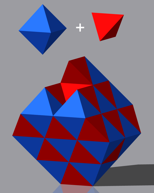
By analogy with the GPS, the coordination of the null-lattice in 3+1 dimensions is 8, with 4 future and 4 past events associated with each node. This may be realized by a lattice with hypercubic structure. That this is the only possibility can be seen by examining flat Minkowski space-time. To this end consider first a spatial hyperplane $P_{0}$ of Minkowski space. The intersection of light-cones from a tetrahedron of adjacent nodes in $P_{0}$ defines a single node in a later hyperplane. To conserve the number of nodes, each node of a spatial hyperplane therefore must be common to 4, otherwise disjoint tetrahedrons. One thus is led to the triangulation of $P_{0}$ by a regular tetrahedral-octahedral honeycomb. The nodes of the hyperplane $P_{0}$ (at ”time” $n_{4}=0$)222In Minkowski space the spatial hyperplanes correspond to global time, but a spatial hypersurface with constant depth $n_{4}$ of Lorentzian space-time in general will not be one to constant cosmic time. thus can be labeled by even integers,

$$P_{0}=\{(2n_{1},2n_{2},2n_{3},0);\ n_{1},n_{2},n_{3}\in\mathbb{Z}\text{ with }n_{1}+n_{2}+n_{3}=0\mod 2\}\ .$$ (4)

This tetrahedral-octahedral tesselation of flat 3-dimensional space with coordination 12 is shown in  Fig. 1a). The 12 spatial neighbors of a node form 4 disjoint sets of 3 that neighbor each other. Together with the common node, these are the vertices of 4 (spatial) tetrahedrons. We will call this a set of F-tetrahedrons (or ”forward” tetrahedrons). In  Fig. 1b) they are colored yellow. The complementary set of 4 (blue in  Fig. 1b)) B-tetrahedrons (or ”backward” tetrahedrons) have the same common node and every edge of a B-tetrahedron also is the edge of an F-tetrahedron, but B- and F- tetrahedrons do not share a face. The vicinity of the node $(0,0,0,0)$ of the lattice $\mathbf{\Lambda}$ includes the following sets of nodes,

$\displaystyle\begin{smallmatrix}(-1,\phantom{-}1,\phantom{-}1,-1)\\ (\phantom{-}1,-1,\phantom{-}1,-1)\\ (\phantom{-}1,\phantom{-}1,-1,-1)\\ (-1,-1,-1,-1)\end{smallmatrix}\begin{smallmatrix}\xrightarrow{\text{illumination}}\\ \xleftarrow{\text{intersection}}\end{smallmatrix}$ $\displaystyle\overbrace{\left.\begin{smallmatrix}(0,\phantom{-}0,\phantom{-}0,\phantom{-}0)&(-2,\phantom{-}2,\phantom{-}0,\phantom{-}0)&(-2,\phantom{-}0,\phantom{-}2,\phantom{-}0)&(0,\phantom{-}2,\phantom{-}2,\phantom{-}0)\\ (2,-2,\phantom{-}0,\phantom{-}0)&(\phantom{-}0,\phantom{-}0,\phantom{-}0,\phantom{-}0)&(\phantom{-}0,-2,\phantom{-}2,\phantom{-}0)&(2,\phantom{-}0,\phantom{-}2,\phantom{-}0)\\ (2,\phantom{-}0,-2,\phantom{-}0)&(\phantom{-}0,\phantom{-}2,-2,\phantom{-}0)&(\phantom{-}0,\phantom{-}0,\phantom{-}0,\phantom{-}0)&(2,\phantom{-}2,\phantom{-}0,\phantom{-}0)\\ (0,-2,-2,\phantom{-}0)&(-2,\phantom{-}0,-2,\phantom{-}0)&(-2,-2,\phantom{-}0,\phantom{-}0)&(0,\phantom{-}0,\phantom{-}0,\phantom{-}0)\end{smallmatrix}\ \right\}}^{\text{B-tetrahedrons}}\text{F-tetrahedrons}$
$\displaystyle\hskip 50.00008pt\text{illumination}\uparrow\downarrow\text{intersection}$
$\displaystyle\hskip 3.00003pt\begin{smallmatrix}(1,-1,-1,\phantom{-}1)&(-1,\phantom{-}1,-1,\phantom{-}1)&(-1,-1,\phantom{-}1,\phantom{-}1)&(1,\phantom{-}1,\phantom{-}1,\phantom{-}1)\end{smallmatrix}\ .$ (5)

If the four nodes of a column/row label the vertices of a B/F- tetrahedron,  Eq.(II) may be interpreted as follows: the forward light cones333To represent Minkowski space by an integer lattice the speed of light may conveniently be taken as $c=1/\sqrt{3}$. of the B-tetrahedron at depth $n_{4}=-1$ illuminate the four F-tetrahedrons (rows) at depth $n_{4}=0$. The events of the selected B-tetrahedron of the $n_{4}=-1$ hyperplane thus are on the backward light cone of the $(0,0,0,0)$ node. Each node at $n_{4}=-1$ is at the intersection of four backward light cones based at the vertices of an F-tetrahedron in the $n_{4}=0$ hyperplane. The rows/columns of the matrix of vertices on the $n_{4}=0$ hyperplane label the vertices of F/B- tetrahedrons with the common node $(0,0,0,0)$. The forward light cones from the vertices of a B-tetrahedron in the $n_{4}=0$ hyperplane intersect at a vertex of the $n_{4}=1$ hyperplane and the corresponding B-tetrahedron is illuminated by this vertex. The four vertices obtained as intersections of light cones from four B-tetrahedrons that include the $(0,0,0,0)$ node form the F-tetrahedron of the $n_{4}=1$ hyperplane in  Eq.(II). Its vertices are on the forward light cone of $(0,0,0,0)$.

Although but a small local section of the whole lattice,  Eq.(II) illustrates the general construction:

  • A spatial Cauchy surface is triangulated by B-tetrahedrons with no common edge. Every vertex of this triangulation is common to four B-tetrahedrons.

  • Vertices of the next spatial hypersurface correspond to the intersection of four forward light cones emanating from the nodes of a B-tetrahedron of the earlier Cauchy surface.

  • The vertices obtained from four B-tetrahedrons with a common node form an F-tetrahedron of the later spatial hypersurface. They lie on the forward light cone of the node that is common to the B-tetrahedrons. Four of these F-tetrahedrons have one node in common but do not share an edge.

  • The corresponding B-tetrahedrons of the later hyperplane share an edge with each of six surrounding F-tetrahedrons.

  • the procedure is repeated to obtain the spatial hypersurface of the next depth. One thus arrives at a foliated causal description of space-time.

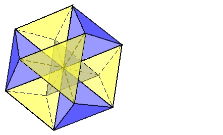
Fig. 2 illustrates the analogous construction in 1+1 and 2+1 space-time dimensions. The hypercubes in 2+1 dimensions are three-dimensional cubes and the tetrahedrons of a spatial hypersurface become triangles of a two-dimensional, hexagonally triangulated surface. Note that the F- and B- triangles individually suffice to determine the (hexagonally) triangulated two-dimensional surface. In 1+1 dimensional space-time the cubes reduce to squares and the (F/B) triangles become line segments that coincide. Note that the number of independent spatial lengths is the number of geometrical degrees of freedom in any dimension, that is $1,3$ and $6$ per node in $d=2,3$ and $4$ dimensions respectively.

Refer to caption
Figure 2: Topological lattices in $1+1$ and $2+1$ space-time dimensions. Forward null vectors are in red and the corresponding backward (B) and forward (F) spatial simplexes are shown in blue and yellow respectively. a) In 1+1 dimensions these spatial simplexes are 1-dimensional and coincide. Forward and backward light-cones are triangles with indicated apexes. Events and their causal relation correspond to nodes and links on this topologically square null-lattice. b) In $2+1$ space-time dimensions the topological null-lattice is cubic and the 2-dimensional spatial hypersurfaces are hexagonally triangulated with coordination 6. [As discussed in the text, the construction of a null-lattice in $3+1$ dimensions is analogous, with hypercubes replacing cubes and tetrahedrons replacing the triangles. The tetrahedral-octahedral triangulation of 3-dimensional spatial hypersurfaces in  Fig. 1 has coordination 12.] The 3(4) vertices of blue B-triangles (tetrahedrons) are the apexes of future light cones (with rays shown in red). Their intersection corresponds to the node of a yellow F-triangle (tetrahedron) on a future Cauchy surface. The subset of F- or B-triangles (tetrahedrons) both triangulate a 2(3)-dimensional Cauchy surface. The triangles (tetrahedrons) of a causal 2(3)+1 dimensional Lorentzian manifold in general are not regular and the lattice is deformed as in a).

We triangulated flat Minkowski space, but the construction can be generalized to causal Lorentzian manifolds. Future events again are at the intersection of (four) forward light-cones from a spatial B-tetrahedron of earlier events, although these B-tetrahedrons generally are not regular. Four spatial B-tetrahedrons with a common event define the events of a future F-tetrahedron. The construction fails if the four light cones emanating from the vertices of a B-tetrahedron do not intersect. With only a finite number of nodes this can occur near curvature singularities such as the singular world line of a black hole or the singular surface of a cosmic string. In the present construction such singular defects can only occur in the critical limit where the number of nodes becomes arbitrary large while the total 4-volume remains finite.

The main challenge will be to ensure that field configurations describe causally triangulated manifolds. Since each space-like edge of a B-tetrahedron is shared with an F-tetrahedron, the endpoints of every spatial edge lie on the backward light cone of a unique future event and on the forward light cone of a unique past event. One can glue the edges of F- and B-tetrahedons to a pure 3-complex only if these (spatial) lengths coincide for the respective past and future 4-simplexes. The Topological Lattice Theories (TLT’s) constructed in  Sect.V and Appendix D ensure this consistency condition is satisfied and allow one to uniquely construct the triangulated causal manifold.

Eq.(II) implies that events of the piecewise linear oriented manifold may be labeled by integer quartets of a hypercubic lattice,

$$\mathbf{\Lambda}=\{\mathbf{n}=\sum_{\mu=1}^{4}n_{\mu}\mathbf{\Delta}_{\mu};\ n_{\mu}\in\mathbb{Z}\}\ ,$$ (6)

with forward lattice displacements,

$$\mathbf{\Delta}_{1}=(1,-1,-1,1),\ \mathbf{\Delta}_{2}=(-1,1,-1,1),\ \mathbf{\Delta}_{3}=(-1,-1,1,1),\ \mathbf{\Delta}_{4}=(1,1,1,1)\ .$$ (7)

The labels of 12 spatially neighboring events of a node on the same hyperplane are found by adding the (12) differences of these displacements to the label of the node. This completes the construction of the topologically hypercubic lattice $\mathbf{\Lambda}$ that labels events of the causal universe.

In an alternate scenario connections and co-frames are placed on separate links. In addition to $\mathbf{\Lambda}$ we in this case consider the lattice with ”time-conjugate” forward displacements,

$$\bar{\mathbf{\Delta}}_{1}=(1,-1,-1,-1),\ \bar{\mathbf{\Delta}}_{2}=(-1,1,-1,-1),\ \bar{\mathbf{\Delta}}_{3}=(-1,-1,1,-1),\ \bar{\mathbf{\Delta}}_{4}=(1,1,1,-1)\ .$$ (8)

By construction these satisfy,

$\displaystyle\mathbf{\Delta}_{\mu}-\mathbf{\Delta}_{\nu}+\bar{\mathbf{\Delta}}_{\nu}-\bar{\mathbf{\Delta}}_{\mu}$ $\displaystyle=0\text{ for all }\ \mu,\nu$
$\displaystyle\mathbf{\Delta}_{\mu}+\mathbf{\Delta}_{\nu}+\bar{\mathbf{\Delta}}_{\rho}+\bar{\mathbf{\Delta}}_{\sigma}$ $\displaystyle=0\text{ for }\ \ \{\mu,\nu,\rho,\sigma\}=\{1,2,3,4\}\ .$ (9)

The displacements of  Eq.(8) and  Eq.(7) are oppositely oriented444The lattice displacements $\{\mathbf{\Delta}_{\mu}\}$ ($\{\bar{\mathbf{\Delta}}_{\mu}\}$) form left(right)-handed systems. and related by the orthogonal matrix $O$ with $\det{O}=-1$,

$$\bar{\mathbf{\Delta}}_{\mu}=\sum_{\nu}O_{\mu\nu}\mathbf{\Delta}_{\nu}\ \ \text{with }O=\frac{1}{2}{\left(\begin{array}[]{rrrr}1&-1&-1&-1\\ -1&1&-1&-1\\ -1&-1&1&-1\\ -1&-1&-1&1\\ \end{array}\right)}\ .$$ (10)

The conjugate forward displacements of  Eq.(8) generate a hypercubic lattice with nodes labeled by,

$$\bar{\mathbf{\Lambda}}=\{\mathbf{n}=\sum_{\mu=1}^{4}n_{\mu}\bar{\mathbf{\Delta}}_{\mu};\ n_{\mu}\in\mathbb{Z}\}\ .$$ (11)

By  Eq.(II), the labels of all ’even’ nodes of $\mathbf{\Lambda}$ and $\bar{\mathbf{\Lambda}}$ coincide and the corresponding events are identified, with

$$\mathbf{\Lambda}\cap\bar{\mathbf{\Lambda}}=\{\mathbf{n}=\sum_{\mu=1}^{4}n_{\mu}\bar{\mathbf{\Delta}}_{\mu};\ \sum^{4}_{\mu=1}n_{\mu}=0\mod 2\}\ .$$ (12)

However, the union $\mathbf{\Lambda}\cup\bar{\mathbf{\Lambda}}$ leaves ’odd’ nodes of $\bar{\mathbf{\Lambda}}$ out in the cold and generally leads to an unstable model. This can be avoided by including a second, translated copy $\mathbf{\Lambda}^{\prime}$ of $\mathbf{\Lambda}$ that coincides with $\bar{\mathbf{\Lambda}}$ at odd nodes,

$$\mathbf{\Lambda}^{\prime}=\{\mathbf{n}=\bar{\mathbf{\Delta}}_{4}+\sum_{\mu=1}^{4}n_{\mu}\mathbf{\Delta}_{\mu};\ n_{\mu}\in\mathbb{Z}\}\ .$$ (13)

The combined lattice,

$$\mathbf{\Lambda}_{d}=\mathbf{\Lambda}\cup\mathbf{\Lambda}^{\prime}\cup\bar{\mathbf{\Lambda}}=\mathbf{\Lambda}\cup\mathbf{\Lambda}^{\prime}\ ,$$ (14)

is the union of the hypercubic lattice $\mathbf{\Lambda}$ with vertices of the $\mathbf{\Lambda}^{\prime}$ lattice at the centers of its cells. This body-centered hypercubic $C_{4}^{2}$ lattice, the 16-cell honeycomb of 4-dimensional Euclidean space, is the 4-dimensional analogue of a body-centered cubic lattice. The Euclidean distance to each of the 24 nearest neighbors of a vertex on this lattice is 2 in the present parameterization and unit 3-spheres whose centers coincide with vertices of $\mathbf{\Lambda}_{d}$ have the densest packing in 4-dimensional Euclidean spaceMusin (2003). The hypercubic sub-lattices $\mathbf{\Lambda}$ and $\mathbf{\Lambda}^{\prime}$ are in dual positions, i.e. $\mathbf{\Lambda}$ could be interpreted as the dual hypercubic lattice to $\mathbf{\Lambda}^{\prime}$. $\bar{\mathbf{\Lambda}}\subset\mathbf{\Lambda}_{d}$ is a hypercubic sub-lattice of $\mathbf{\Lambda}_{d}$ whose even and odd nodes coincide with nodes of $\mathbf{\Lambda}$ and $\mathbf{\Lambda}^{\prime}$ respectively.

Inclusion of the dual hypercubic lattice leads to a more symmetric and appealing construction at the price of ”doubling” the number of causally connected components. Locally, the two components, $\mathbf{\Lambda}$ and $\mathbf{\Lambda}^{\prime}$, of the ”duoverse” $\mathbf{\Lambda}_{d}$ are causally disjoint although the space-time geometry of each connected component will be determined by the field content on both. From the point of view of one of its causally connected components, the duoverse $\mathbf{\Lambda}_{d}$ resembles a single universe constructed on $\mathbf{\Lambda}$ only. The (gravitational) field content of both scenarios in fact is the same.

III Fields and Observables

To obtain the Lorentzian lattice model with causal dynamics, consider first the topologically hypercubic lattice $\mathbf{\Lambda}$ of the universe. For the duoverse a similar construction holds on the hypercubic $\bar{\mathbf{\Lambda}}$ sub-lattice.

Links are ordered pairs of neighboring nodes of $\mathbf{\Lambda}$. We adopt standard conventions and use $[\mathbf{n},\mathbf{n}^{\prime}]\ \text{or }[\mathbf{n},\mathbf{n}+\mathbf{\Delta}_{\mu}]\equiv[\mathbf{n},\mathbf{n}+\mu]\equiv[\mathbf{n},\mu]$ to identify links of $\mathbf{\Lambda}$ - whichever notation is more convenient. $\mathbf{\Lambda}$ is naturally oriented by the displacements of  Eq.(7). Links $[\mathbf{n}+\mu,\mathbf{n}]\equiv[\mathbf{n}+\mu,-\mu]$ are said to be reversed. Sometimes more general paths $[\mathbf{n}_{0},\mathbf{n}_{1},\mathbf{n}_{2},\dots]$ have to be considered. They are given by a contiguous set of oriented links $[\mathbf{n}_{i},\mathbf{n}_{i+1}]\in\mathbf{\Lambda}$.

The variables $E^{AA^{\prime}}_{\mu}(\mathbf{n})$ of this lattice formulation are a finite lattice version of the continuum 1-form $e^{AA^{\prime}}_{k}(\mathbf{n})dx^{k}$ in spinorial representationPenrose and MacCallum (1973). The differential $dx^{k}$ is represented by a contravariant vector $l^{k}_{\mu}$ that approximates the ”displacement” to the node $\mathbf{n}+\mu$ along the geodesic ${\cal C}[\mathbf{n},\mathbf{n}+\mu]$ between the two events,

$$E^{AA^{\prime}}_{\mu}(\mathbf{n}):=e^{AA^{\prime}}_{k}(\mathbf{n})l^{k}_{\mu}(\mathbf{n})\sim\left.e^{AA^{\prime}}_{k}\frac{dx^{k}}{d\lambda}\right|_{\mathbf{n}}\frac{\Delta\lambda}{l_{P}}\ .$$ (15)

The contravariant displacement vector $l^{k}_{\mu}$ is uniquely defined using the affine parametrization of a geodesic with $x(\lambda=0)\equiv x(\mathbf{n})$ and $x(\lambda=1)\equiv x(\mathbf{n}+\mu)$ and $\Delta\lambda=1$. In natural units it is the tangent $u^{k}_{\mu}(\lambda=0)=u^{k}_{\mu}(\mathbf{n})$ to the so affine parameterized geodesic ${\cal C}[\mathbf{n},\mathbf{n}+\mu]$ joining the two events555This geometric interpretation of $E^{AA^{\prime}}_{\mu}(\mathbf{n})$ is owedcom (2016) to T. Jacobson.,

$$l^{k}_{\mu}(\mathbf{n})=\frac{1}{l_{P}}\left.\frac{dx^{k}}{d\lambda}\right|_{{\cal C}[\mathbf{n},\mathbf{n}+\mu]}(\lambda=0):=\frac{1}{l_{P}}u^{k}_{\mu}(\mathbf{n})\ .$$ (16)

The dimension of the displacement vector has here been absorbed by $l_{P}$ so that all variables of the lattice model are dimensionless. We effectively are measuring length in units of $l_{P}=\sqrt{32\pi\hbar G/c^{3}}\approx 1.6\times 10^{-34}m$, time in units of $l_{P}/c$ and energy in units of $\hbar c/l_{P}$. $l_{P}$ here is a dimensional unit on the same footing as $\hbar$ and $c$. The only gravitational coupling of this lattice model is the dimensionless cosmological constant $\lambda=\Lambda l_{P}^{2}$. It plays a rôle analogous to that of the (in 3+1 dimensional space-time) dimensionless couplings $\alpha=e^{2}/(\hbar c)$ and $g^{2}$ of the electro-weak and strong interactions.

The displacement vector $l^{k}_{\mu}(\mathbf{n})$ of  Eq.(16) for given events $\mathbf{n}$ and $\mathbf{n}+\mu$ is a (uniquely defined) contravariant vector and its contraction with the co-frame $e^{AA^{\prime}}_{k}(\mathbf{n})$ to $E_{\mu}(\mathbf{n})$ in  Eq.(15) is a scalar. A smooth change of coordinates in the vicinity of the event $\mathbf{n}$ in particular transforms $l^{k}_{\mu}(\mathbf{n})$ and the co-frame $e_{k}(\mathbf{n})$, but not $E_{\mu}(\mathbf{n})$. For lack of a better name, we refer to $\{E_{\mu}(\mathbf{n}),\mu=1,\dots,4\}$ as a lat-frame at the node $\mathbf{n}$, even though this ”frame” is parametrization invariant.

In Appendix B first order actions for spinors, scalars and gauge fields are written in terms of (diffeomorphism invariant) forms. Displacements and co-frames thus never appear separately and the corresponding actions for the discretized model can be written in terms of lat-frames only. This is desirable, since the diffeomorphism group does not act on the triangulation of a continuous manifold by a finite number of points. Apart from an internal $SL(2,\mathbb{C})\,$symmetry, the present lattice model thus is a dynamical triangulation that preserves coordination number.

The matrices $E_{\mu}(\mathbf{n})$ transform homogeneously under local $SL(2,\mathbb{C})\,$transformations,

$$E_{\mu}(\mathbf{n})\longrightarrow g(\mathbf{n})E_{\mu}(\mathbf{n})g^{\dagger}(\mathbf{n})\ \ \text{ with }g(\mathbf{n})\in\textrm{$SL(2,\mathbb{C})\,$}\ ,$$ (17)

and the $SL(2,\mathbb{C})\,$invariant inner product on this space of anti-hermitian matrices is,

$$X\cdot Y:=-{\textstyle\frac{1}{2}}{\rm Tr}\varepsilon X^{T}\varepsilon Y=-{\textstyle\frac{1}{2}}X^{AB^{\prime}}\varepsilon_{AB}Y^{BA^{\prime}}\varepsilon_{A^{\prime}B^{\prime}}\in\mathbb{R}$$ (18)

where $X^{T}=-X^{*}$ denotes the transpose of the anti-hermitian matrix $X=-X^{\dagger}$ and $\varepsilon=\left(\begin{smallmatrix}0&1\\ -1&0\end{smallmatrix}\right)$ is the $SL(2,\mathbb{C})\,$invariant tensor.

It sometimes is more convenient to consider lat-frames as $so^{+}(3,1)$ vectors. The relation to their spinorial representation is provided by an orthogonal basis of anti-hermitian $2\times 2$ matrices666We in particular consider a basis in which the $\vec{\sigma}=(\sigma_{1},\sigma_{2},\sigma_{3})$-matrices are traceless anti-hermitian generators of an $su(2)$ algebra and $\sigma_{4}=i{\mathbb{1}}$.,

$$\{\sigma^{AB^{\prime}}_{a},a=1,\dots,4;\sigma_{a}=-\sigma_{a}^{\dagger}\ \text{with }\ {\rm Tr}\,\sigma^{a}\sigma_{b}=2\delta^{a}_{b},\text{ where}\ \sigma^{a}_{A^{\prime}B}:=\varepsilon_{BC}\sigma^{CC^{\prime}}_{a}\varepsilon_{C^{\prime}A^{\prime}}\}.$$ (19)

The spinor and vector components of lat-frames are related by,

$$E^{AB^{\prime}}_{\mu}(\mathbf{n})=\sum_{a=1}^{4}\sigma_{a}^{AB^{\prime}}E^{a}_{\mu}(\mathbf{n});\ E^{a}_{\mu}={\textstyle\frac{1}{2}}{\rm Tr}\sigma^{a}E_{\mu}\ .$$ (20)

and the scalar product of  Eq.(18) in the vector representation is,

$$X\cdot Y=X^{a}\eta_{ab}X^{b}\ ,$$ (21)

with $\eta_{ab}=\text{diag}(1,1,1,-1)$  .

As discussed previously, to ensure causality and in analogy with the GPS, all forward displacements are chosen light-like,

$$E_{\mu}(\mathbf{n})\cdot E_{\mu}(\mathbf{n})=g_{jk}(\mathbf{n})l^{j}_{\mu}(\mathbf{n})l^{k}_{\mu}(\mathbf{n})=0\ \text{ with }\ -i{\rm Tr}E_{\mu}>0\ .$$ (22)

The same causal manifold may be triangulated in a number of ways, but its triangulation by a topological null-lattice is unique up to the placement of events on the boundary of the manifold. [For a more detailed discussion of a conic manifold see Appendix E.]

Up to $SL(2,\mathbb{C})\,$transformations, a null lat-frame represents the 6 spatial distances $\ell_{\mu\nu}(\mathbf{n})>0$ between four events on the forward light-cone of $\mathbf{n}$,

$$\ell^{2}_{\mu\nu}(\mathbf{n})=(E_{\mu}-E_{\nu})\cdot(E_{\mu}-E_{\nu})=-2E_{\mu}(\mathbf{n})\cdot E_{\nu}(\mathbf{n})=-2g_{ik}(\mathbf{n})l^{i}_{\mu}(\mathbf{n})l^{k}_{\nu}(\mathbf{n})\geq 0\ .$$ (23)

These lengths are coordinate invariant geometrical quantities. Modulo $SL(2,\mathbb{C})\,$transformation, a null lat-frame thus describes $6$ geometric degrees of freedom.

In general, lat-frames are not proportional to the co-frames in any coordinate system777The displacement matrices $l^{k}_{\mu}(\mathbf{n})$ generally do not correspond to a smooth coordinate transformation $\partial x^{k}/\partial x^{\prime\mu}(\mathbf{n})$ at more than one node.. However, they may be identified with (forward) null co-frames in Minkowski space-time888The null lat-frames for instance can be taken proportional to co-frames of the system $S^{\prime}$ related to Minkowski space with metric $g_{ik}=\text{diag}(1,1,1,-1)$ by the linear coordinate transformation $4x^{\prime 1}=-x^{1}+x^{2}+x^{3}+x^{4}/\sqrt{3},\ 4x^{\prime 2}=x^{1}-x^{2}+x^{3}+x^{4}/\sqrt{3},\ 4x^{\prime 3}=x^{1}+x^{2}-x^{3}+x^{4}/\sqrt{3},4x^{\prime 4}=-x^{1}-x^{2}-x^{3}+x^{4}/\sqrt{3}$. This transformation preserves orientation and, as required by  Eq.(23), scalar products of the lat-frames are negative semi-definite. The metric in $S^{\prime}$ is $g^{\prime}_{\mu\nu}=E^{\text{Mink}}_{\mu}\cdot E^{\text{Mink}}_{\nu}=-4$ for $\mu\neq\nu$ and vanishes for $\mu=\nu$., for instance,

$$E^{\text{Mink}}_{1}=i\left(\begin{smallmatrix}\sqrt{3}+1&-1+i\\ -1-i&\sqrt{3}-1\\ \end{smallmatrix}\right),\ E^{\text{Mink}}_{2}=i\left(\begin{smallmatrix}\sqrt{3}+1&1-i\\ 1+i&\sqrt{3}-1\\ \end{smallmatrix}\right),\ E^{\text{Mink}}_{3}=i\left(\begin{smallmatrix}\sqrt{3}-1&1+i\\ 1-i&\sqrt{3}+1\\ \end{smallmatrix}\right),\ E^{\text{Mink}}_{4}=i\left(\begin{smallmatrix}\sqrt{3}-1&-1-i\\ -1+i&\sqrt{3}+1\\ \end{smallmatrix}\right).$$ (24)

$SL(2,\mathbb{C})\,$-transformed and scaled null lat-frames give an equivalent description of discretized Minkowski space-time. Note that the lattice displacement vectors in $S^{\prime}$ are $l^{k}_{\mu}=a\delta^{k}_{\mu}$. The global lattice constant $a$ gives the coarseness of the discretization (in units of $l_{P}$). This reflects the possibility of choosing a local inertial system that describes the immediate neighborhood of an event. The resulting piecewise linear approximation to a smooth manifold can be justified for a sufficiently ”fine” lattice, but fails to reproduce curvature singularities. These singularities may only be recovered in the critical limit where the number of events becomes infinite.

Eq.(18) and  Eq.(22) imply that null lat-frames are singular matrices and may be represented by complex bosonic 2-component spinors $\xi^{A}_{k},\,(A=1,2)$,-

$$E_{\mu}^{AB^{\prime}}(\mathbf{n})=i(\xi_{\mu}\otimes\xi^{*}_{\mu})_{\mathbf{n}}^{AB^{\prime}}=i\xi_{\mu}^{A}(\mathbf{n})\xi^{*B^{\prime}}_{\mu}(\mathbf{n})\ ,$$ (25)

where $\xi^{*}_{\mu}$ denotes the complex conjugate spinor. A primed upper case Latin index indicates that the spinor transforms with the complex conjugate representation of $SL(2,\mathbb{C})\,$. There is no summation over the repeated Greek index999Only diagonally related, repeated indices, i.e. ${}_{A}\!\!\nearrow^{A}$ and ${}^{B}\!\!\searrow_{B}$, are summed. $\mu$ in  Eq.(25). Components of the conjugate $\chi^{c}$ of any spinor $\chi$ are,

$$\chi^{c}_{A}:=\chi^{B}\varepsilon_{BA}\ .$$ (26)

$\xi_{\mu}(\mathbf{n})$ and its conjugate $\xi^{c}_{\mu}(\mathbf{n})$ thus transform inversely under $SL(2,\mathbb{C})\,$,

$$\xi^{A}_{\mu}(\mathbf{n})\longrightarrow g^{A}_{\ B}(\mathbf{n})\xi^{B}_{\mu}(\mathbf{n})\ \Leftrightarrow\ \xi^{c}_{\mu\,A}(\mathbf{n})\longrightarrow\xi^{c}_{\mu\,B}(\mathbf{n})g^{-1B}_{\ \ \ \ A}(\mathbf{n}),\text{ for }g(\mathbf{n})\in\textrm{$SL(2,\mathbb{C})\,$}\ .$$ (27)

A lat-frame in addition is invariant under local $U^{4}(1)$ phase transformations of the spinors,

$$\xi_{\mu}(\mathbf{n})\rightarrow\xi^{\prime}_{\mu}(\mathbf{n})=e^{-i\psi_{\mu}(\mathbf{n})}\xi_{\mu}(\mathbf{n})\text{ and }\xi^{*}_{\mu}(\mathbf{n})\rightarrow\xi^{\prime*}_{\mu}(\mathbf{n})=e^{i\psi_{\mu}(\mathbf{n})}\xi^{*}_{\mu}(\mathbf{n}),\ \ \psi_{\mu}(\mathbf{n})\in\mathbb{R}\ .$$ (28)

A spinor may be compared to another by parallel transport along links of the lattice to a common node. The parallel transport of a spinor from $\mathbf{n}+\Delta_{\mu}$ to $\mathbf{n}$ is given by matrix $U_{\mu}(\mathbf{n})\equiv U[\mathbf{n},\mu]\equiv U[\mathbf{n},\mathbf{n}+\Delta_{\mu}]\in\textrm{$SL(2,\mathbb{C})\,$}$. Nodes of the lattice thus are associated with four spinors and its oriented links $[\mathbf{n},\mu]$ with parallel transport matrices. On a (periodic) hypercubic null-lattice with $N$ nodes there are altogether $4N$ spinors and $4N$ transport matrices. Under the $SL(2,\mathbb{C})\,$structure group the transport matrices transform as ($g(\mathbf{n})\in\textrm{$SL(2,\mathbb{C})\,$}$),

$$U^{A}_{\mu B}(\mathbf{n})\rightarrow g^{A}_{\ C}(\mathbf{n})U^{C}_{\mu D}(\mathbf{n})g^{-1D}_{\ \ \ \ B}(\mathbf{n}+\mu)\ .$$ (29)

Although consistent with  Eq.(29), the reversed lattice link will not be associated with the inverse-, but rather with the hermitian conjugate transport matrix,

$$U[\mathbf{n},\mathbf{n}^{\prime}]=U^{\dagger}[\mathbf{n}^{\prime},\mathbf{n}]\ .$$ (30)

Since the representation of $SL(2,\mathbb{C})\,$ is not unitary,  Eq.(30) eliminates closed (Wilson) loops of $SL(2,\mathbb{C})\,$transport matrices101010The identification $U[\mathbf{n},\mathbf{n}^{\prime}]=U^{-1}[\mathbf{n}^{\prime},\mathbf{n}]$ would include closed (Wilson) loops of the form ${\rm Tr}U[\mathbf{n}_{1},\mathbf{n}_{2}]U[\mathbf{n}_{2},\mathbf{n}_{3}]\dots U[\mathbf{n}_{r},\mathbf{n}_{1}]$ as basic $SL(2,\mathbb{C})\,$invariants. from the $SL(2,\mathbb{C})\,$-invariant observables one can construct for this lattice. Eqs. (27), (29) and (30) imply that the basic $SL(2,\mathbb{C})\,$invariants of this model are contiguous strings of transport matrices bookended by spinors,

$$I_{\mu\nu}^{(r)}[\mathbf{n}_{0},\mathbf{n}_{1},\dots,\mathbf{n}_{r}]:=\xi^{c}_{\mu}(\mathbf{n}_{0})U[\mathbf{n}_{0},\mathbf{n}_{1}]U[\mathbf{n}_{1},\mathbf{n}_{2}]\dots U[\mathbf{n}_{r-1},\mathbf{n}_{r}]\xi_{\nu}(\mathbf{n}_{r})\ ,$$ (31)

where $[\mathbf{n}_{0},\mathbf{n}_{1},\dots,\mathbf{n}_{r}]$ is a continuous chain of forward oriented links. For reference we separately list and name the three shortest invariants,

$\displaystyle f_{\mu\nu}(\mathbf{n})$ $\displaystyle:=\xi^{c}_{\mu A}(\mathbf{n})\xi^{A}_{\nu}(\mathbf{n})\equiv\xi^{c}_{\mu}(\mathbf{n})\xi_{\nu}(\mathbf{n})=:I_{ij}^{(0)}[\mathbf{n}]\ ,$ (32a)
$\displaystyle\psi_{\mu\nu\rho}(\mathbf{n})$ $\displaystyle:=\xi^{c}_{\mu A}(\mathbf{n})U^{A}_{\rho B}(\mathbf{n})\xi^{B}_{\nu}(\mathbf{n}+\rho)\equiv\xi^{c}_{\mu}(\mathbf{n})U[\mathbf{n},\mathbf{n}_{1}]\xi_{\nu}(\mathbf{n}_{1})=:I_{\mu\nu}^{(1)}[\mathbf{n},\mathbf{n}+\rho]\ ,$ (32b)
$\displaystyle\chi_{\mu\nu\rho\sigma}(\mathbf{n})$ $\displaystyle:=\xi^{c}_{\mu A}(\mathbf{n})U^{A}_{\rho B}(\mathbf{n})U^{B}_{\sigma C}(\mathbf{n}+\rho)\xi^{C}_{\nu}(\mathbf{n}+\rho+\sigma)$
$\displaystyle\hskip 30.00005pt\equiv\xi^{c}_{\mu}(\mathbf{n})U[\mathbf{n},\mathbf{n}_{1}]U[\mathbf{n}_{1},\mathbf{n}_{2}]\xi_{\nu}(\mathbf{n}_{2})=:I_{\mu\nu}^{(2)}[\mathbf{n},\mathbf{n}+\rho,\mathbf{n}+\rho+\sigma]\ .$ (32c)

The invariants of Eqs. (31) and (32) in general are complex and physical observables necessarily depend on the corresponding complex conjugate invariants as well. The path of the latter is reversed and they are bookended by hermitian conjugate spinors. Invariance under the local $U^{4}(1)$ phase transformations of  Eq.(28) implies that physical observables locally conserve four separate spinor numbers. They thus depend only on the null lat-frames of  Eq.(25).  Sect.V.2 exploits the $U^{4}(1)$ symmetry to construct a local TLT that constrains the space of lattice spinor configurations to those that correspond to triangulated causal manifolds.

The magnitude of the symplectic form $f_{\mu\nu}(\mathbf{n})=-f_{\nu\mu}(\mathbf{n})$ on the space of spinors at site $\mathbf{n}$ is the spatial length $\ell^{2}_{\mu\nu}(\mathbf{n})$ of  Eq.(23),

$$\ell^{2}_{\mu\nu}(\mathbf{n})={\rm Tr}\varepsilon E^{T}_{\mu}(\mathbf{n})\varepsilon E_{\nu}(\mathbf{n})=|f_{\mu\nu}(\mathbf{n})|^{2}\geq 0\ ,$$ (33)

where we used Eqs. (25) and (32a). Note that the length $\ell^{2}_{\mu\nu}$ vanishes only if the two spinors $\xi_{\mu}$ and $\xi_{\nu}$ are linearly dependent.

In four dimensions the 6 complex variables of the anti-symmetric matrix $f_{\mu\nu}(\mathbf{n})$ are constrained by the fact that its Pfaffian vanishes,

$$\text{Pf}(f(\mathbf{n})):=\frac{1}{8}\sum_{\mu\nu\rho\sigma}\varepsilon(\mu\nu\rho\sigma)f_{\mu\nu}(\mathbf{n})f_{\rho\sigma}(\mathbf{n})=f_{12}(\mathbf{n})f_{34}(\mathbf{n})+f_{13}(\mathbf{n})f_{42}(\mathbf{n})+f_{14}(\mathbf{n})f_{23}(\mathbf{n})=0\ .$$ (34)

The matrix $f(\mathbf{n})$ thus depends on 10 real parameters only. Four of these are overall phases of the spinorsPenrose and MacCallum (1973) (see  Eq.(28)). The remaining 6 real degrees of freedom are the spatial lengths $\ell_{\mu\nu}(\mathbf{n})\geq 0$ of  Eq.(33).

The vanishing Pfaffian implies that the magnitudes of the three complex numbers in  Eq.(34) satisfy triangle inequalities,

$$0\leq a(\mathbf{n})\leq b(\mathbf{n})+c(\mathbf{n}),\ \ \ 0\leq b(\mathbf{n})\leq c(\mathbf{n})+a(\mathbf{n}),\ \ \ 0\leq c(\mathbf{n})\leq a(\mathbf{n})+b(\mathbf{n})\ ,$$ (35)

with,

$\displaystyle a(\mathbf{n}):=$ $\displaystyle\ell_{12}(\mathbf{n})\ell_{34}(\mathbf{n})=|f_{12}(\mathbf{n})f_{34}(\mathbf{n})|$
$\displaystyle b(\mathbf{n}):=$ $\displaystyle\ell_{13}(\mathbf{n})\ell_{24}(\mathbf{n})=|f_{13}(\mathbf{n})f_{42}(\mathbf{n})|$
$\displaystyle c(\mathbf{n}):=$ $\displaystyle\ell_{14}(\mathbf{n})\ell_{23}(\mathbf{n})=|f_{14}(\mathbf{n})f_{23}(\mathbf{n})|\ .$ (36)

For non-negative $a,b$, and $c$, the triangle inequalities of  Eq.(35) can be combined to the single inequality,

$$0\geq\left.a^{4}+b^{4}+c^{4}-2a^{2}b^{2}-2b^{2}c^{2}-2c^{2}a^{2}\right|_{\mathbf{n}}=\det{\ell^{2}_{\mu\nu}(\mathbf{n})}\ .$$ (37)

The triangle inequalities of  Eq.(35) thus are equivalent to requiring that the local four volume $V(\mathbf{n})=\sqrt{-\det{\ell^{2}_{\mu\nu}(\mathbf{n})}}$ be real. The fact that causality restricts the spatial lengths $\ell_{\mu\nu}(\mathbf{n})$ so simply is one reason for considering null lat-frames. The converse holds as well: given six non-vanishing positive lengths $\{\ell_{\nu\mu}=\ell_{\mu\nu}>0,1\leq\mu<\nu\leq 4\}$ with $\det{\ell^{2}_{\mu\nu}}\leq 0$, an anti-symmetric complex matrix $f_{\mu\nu}$ with $|f_{\mu\nu}|=\ell_{\mu\nu}$ can be constructed whose Pfaffian vanishes. The spinors then are reconstructed as follows.

The vanishing Pfaffian of  Eq.(34) implies that $f_{\mu\nu}(\mathbf{n})$ and its dual $f^{\mu\nu}(\mathbf{n}):={\textstyle\frac{1}{2}}\sum_{\rho\sigma}\epsilon(\mu\nu\rho\sigma)f_{\rho\sigma}(\mathbf{n})$ are antisymmetric $4\times 4$ matrices of rank 2. The null space of $f^{\mu\nu}(\mathbf{n})$ thus is spanned by two linearly independent vectors $\xi_{\mu}^{A}$,

$$\sum_{\nu}f^{\mu\nu}(\mathbf{n})\xi_{\nu}^{A}(\mathbf{n})=0,\ \text{for}\ A=1,2\ .$$ (38)

Up to normalization these define $f_{\mu\nu}(\mathbf{n})$ itself. The fact that any 4-dimensional anti-symmetric matrix with vanishing Pfaffian is represented by a set of spinors is exploited in  Sect.V and Appendix C.

IV Field Assignments and Lattice Actions

The model is completed by assigning this field content to links and nodes of the lattice and constructing the lattice action and integration measure. We will consider two distinct scenarios:

IV.1 The Universe

Only the hypercubic $\mathbf{\Lambda}$ lattice of  Eq.(6) is utilized in this case. Each of its oriented links $[\mathbf{n},\mu]$ is associated with an $SL(2,\mathbb{C})\,$transport matrix $U_{\mu}(\mathbf{n})$. The reversed link is associated with the hermitian conjugate transport matrix $U^{\dagger}_{\mu}(\mathbf{n})$ as in  Eq.(30).

Each node $\mathbf{n}\in\mathbf{\Lambda}$ furthermore is associated with a null lat-frame $\{E_{\mu}(\mathbf{n}),\;\mu=1,\dots,4\}$ that gives the light-like displacements in the forward direction from $\mathbf{n}$ to the events $\{\mathbf{n}+\mathbf{\Delta}_{\mu},\mu=1,\dots,4\}$.

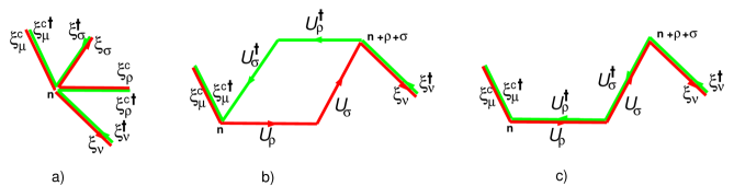
The lattice action is constructed from purely imaginary $SL(2,\mathbb{C})\,$invariant lattice 4-forms with real coefficients. The two most local candidates for the lattice action are,

$\displaystyle\mathcal{V}_{\mu\nu\rho\sigma}(\mathbf{n}):=$ $\displaystyle{\rm Tr}E_{\mu}(\mathbf{n})\varepsilon E^{T}_{\nu}(\mathbf{n})\varepsilon E_{\rho}(\mathbf{n})\varepsilon E^{T}_{\sigma}(\mathbf{n})\varepsilon=2i\varepsilon(\mu\nu\rho\sigma)\det[E]:=2i\varepsilon(\mu\nu\rho\sigma)V(\mathbf{n})$
$\displaystyle=$ $\displaystyle f^{*}_{\mu\nu}(\mathbf{n})f_{\nu\rho}(\mathbf{n})f^{*}_{\rho\sigma}(\mathbf{n})f_{\sigma\mu}(\mathbf{n})\ ,$ (39a)
$\displaystyle{\cal P}_{\mu\nu\rho\sigma}(\mathbf{n}):=$ $\displaystyle\chi_{\mu\nu\rho\sigma}(\mathbf{n})\chi^{*}_{\mu\nu\sigma\rho}(\mathbf{n})={\rm Tr}\varepsilon E^{T}_{\mu}(\mathbf{n})\varepsilon U_{\rho}(\mathbf{n})U_{\sigma}(\mathbf{n}+\rho)E_{\nu}(\mathbf{n}+\rho+\sigma)U^{\dagger}_{\rho}(\mathbf{n}+\sigma)U^{\dagger}_{\sigma}(\mathbf{n})$
$\displaystyle=$ $\displaystyle\xi^{c}_{\mu A}(\mathbf{n})U^{A}_{\rho B}(\mathbf{n})U^{B}_{\sigma C}(\mathbf{n}+\rho)\xi^{C}_{\nu}(\mathbf{n}+\rho+\sigma)\xi^{*\dot{C}}_{\nu}(\mathbf{n}+\sigma+\rho)U_{\rho\dot{C}}^{*\ \dot{B}}(\mathbf{n}+\sigma)U_{\sigma\dot{B}}^{*\ \dot{A}}(\mathbf{n})\xi^{*c}_{\mu\dot{A}}(\mathbf{n})\ ,$ (39b)

These contributions to the action are depicted graphically in Figs. 3a) and 3b) respectively.

Refer to caption
Figure 3: Quasi-local contributions to the invariant action on a null-lattice in $d=3+1$ dimensions. a) The cosmological term $\mathcal{V}_{\mu\nu\rho\sigma}(\mathbf{n})$ at site $\mathbf{n}$ of  Eq.(39). Spinors $\xi_{\mu}(\mathbf{n})$ are shown as red segments along lattice direction $\mu$, hermitian conjugate spinors $\xi^{\dagger}_{\mu}$ are depicted in green. Color flows from conjugate spinors $\xi^{c}_{\mu}$ defined by Eq.(26) to spinors $\xi_{\nu}$ and from $\xi^{\dagger}_{\nu}$ to $\xi^{c\,\dagger}_{\mu}$. Two directed line segments of the same color joined at $\mathbf{n}$ form the $SL(2,\mathbb{C})\,$-invariant (red) $f_{\mu\nu}(\mathbf{n})$ of Eq.(32a) (or its complex conjugate (green)). The contribution to the cosmological term of site $\mathbf{n}$ is the product of these invariants with the sign determined by the permutation of $(\mu\nu\rho\sigma)$. b) The ${\cal P}_{\mu\nu\rho\sigma}(\mathbf{n})$ curvature contribution to  Eq.(39). The depiction of spinors at sites $\mathbf{n}$ and $\mathbf{n}+\rho+\sigma$ is as in a), but these now are parallel transported along links in $\rho$- and $\sigma$- direction by $SL(2,\mathbb{C})\,$transport matrices as shown. The (red) spinors $\xi_{\mu}$ are parallel transported by the $SL(2,\mathbb{C})\,$-matrices $U$, whereas their (green) hermitian conjugates counterparts $\xi^{\dagger}_{\mu}$ are transported by the hermitian conjugate $SL(2,\mathbb{C})\,$-matrices $U^{\dagger}\neq U^{-1}$. The contribution to the lattice Hilbert-Palatini action is given by the product of these two overlaps with a sign determined by the permutation of $(\mu\nu\rho\sigma)$. c) The ${\cal Q}_{\mu\nu\rho\sigma}$ topological term of  Eq.(40). In the continuum limit his term does not affect classical equations of motion and could be included in the lattice action with a purely imaginary coefficient. Similar to the cosmological contribution a), the corresponding path does not enclose a plaquette and does not measure local curvature.

The other two quasi-local observables,

$\displaystyle\ell^{2}_{\mu\nu}(\mathbf{n}):=$ $\displaystyle{\rm Tr}\varepsilon E^{T}_{\mu}(\mathbf{n})\varepsilon E_{\nu}(\mathbf{n})=|f_{\mu\nu}(\mathbf{n})|^{2}=\ell^{2}_{\nu\mu}(\mathbf{n})$ (40a)
$\displaystyle{\cal Q}_{\mu\nu\rho\sigma}(\mathbf{n}):=$ $\displaystyle|\chi_{\mu\nu\rho\sigma}(\mathbf{n})|^{2}={\rm Tr}\varepsilon E^{T}_{\mu}(\mathbf{n})\varepsilon U_{\rho}(\mathbf{n})U_{\sigma}(\mathbf{n}+\rho)E_{\nu}(\mathbf{n}+\rho+\sigma)U^{\dagger}_{\sigma}(\mathbf{n}+\rho)U^{\dagger}_{\rho}(\mathbf{n})$
$\displaystyle=$ $\displaystyle\xi^{c}_{\mu A}(\mathbf{n})U^{A}_{\rho B}(\mathbf{n})U^{B}_{\sigma C}(\mathbf{n}+\rho)\xi^{C}_{\nu}(\mathbf{n}+\rho+\sigma)\xi^{*\dot{C}}_{\nu}(\mathbf{n}+\sigma+\rho)U^{*\ \dot{B}}_{\sigma\dot{C}}(\mathbf{n}+\rho)U^{*\ \dot{A}}_{\rho\dot{B}}(\mathbf{n})\xi^{*c}_{\mu\dot{A}}(\mathbf{n})\ ,$ (40b)

are real. The first of these invariants are the spatial lengths of  Eq.(33) and is symmetric in its indices. The totally anti-symmetric part of ${\cal Q}_{\mu\nu\rho\sigma}(\mathbf{n})$ is the lattice analog of a topological contribution to the continuum action. This term could be (and its continuum analog often isHolst (1996); Ashtekar (1986); Kaul and Sengupta (2012)) included but will not be considered in the following. We furthermore do not investigate other, less local, contributions to the lattice action. The invariant (real) lattice action111111The weight $e^{iS^{\text{inv.}}_{\text{HP}}}$ of a configuration is a pure phase. for a causally connected universe thus is,

$$S^{\text{uni.}}_{\text{HP}}=i\sum_{\mu\nu\rho\sigma}\varepsilon(\mu\nu\rho\sigma)\sum_{\mathbf{n}\in\mathbf{\Lambda}}[\mathcal{P}_{\mu\nu\rho\sigma}(\mathbf{n})+\frac{\lambda}{12}\mathcal{V}_{\mu\nu\rho\sigma}(\mathbf{n})]\ ,$$ (41)

where $\lambda$ is the dimensionless cosmological constant. We have absorbed the coefficient (and dimensionality) of the curvature term in the normalization of the spinors (or equivalently, of the lat-frame $E_{\mu}$). On a hypercubic lattice the HP-action takes the same form whether the lat-frame is light-like or not, but the relation between events of $\mathbf{\Lambda}$ in general would be acausal. Null lat-frames assure causality, but only a subset of such lattice configurations corresponds to triangulated manifolds (see  Sect.V).

IV.2 The Duoverse

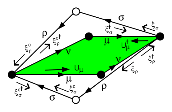
The duoverse is obtained by placing the field content on the lattice $\mathbf{\Lambda}_{d}$ of  Eq.(14). In some ways this scenario is more restrictive and appealing than the universe. In analogy with optics, nodes $\mathbf{n}\in\bar{\mathbf{\Lambda}}$ of the hypercubic sub-lattice $\bar{\mathbf{\Lambda}}\subset\mathbf{\Lambda}_{d}$ will be referred to as ”active” nodes. All other nodes $\bar{\mathbf{n}}\in\mathbf{\Lambda}_{d}\backslash\bar{\mathbf{\Lambda}}$ of $\mathbf{\Lambda}_{d}$ are ”passive” or inert in this construction. In Table 1 and  Fig. 4, active nodes are denoted by solid dots and passive ones by open circles. Half the nodes of $\mathbf{\Lambda}$ and $\mathbf{\Lambda}^{\prime}$ are passive. Active links are between two active nodes whereas passive links are between an active and a passive node. The hypercubic sub-lattices $\mathbf{\Lambda}$ and $\mathbf{\Lambda}^{\prime}$ are composed of passive links only. Depending on whether the initial or final node is active, oriented passive links are of two kinds $[\mathbf{n},\bar{\mathbf{n}}]$ and $[\bar{\mathbf{n}},\mathbf{n}]$. There are no links between two passive nodes in this construction. $SL(2,\mathbb{C})\,$transport matrices $U_{\mu}(\mathbf{n})$ reside on oriented active links $[\mathbf{n},\mathbf{n}^{\prime}=\mathbf{n}+\bar{\mathbf{\Delta}}_{\mu}]\in\bar{\mathbf{\Lambda}}$ only. The reversed active link being associated with the hermitian conjugate transport matrix as in  Eq.(30) and Table 1.  Fig. 4 depicts these assignments for a $\rho\sigma$-plaquette of $\mathbf{\Lambda}$ (or $\mathbf{\Lambda}^{\prime}$) and a $\mu\nu$-plaquette of $\bar{\mathbf{\Lambda}}$ that have two active nodes in common.

 $$\begin{array}[]{c|c|c}&\text{\ \ \ oriented \ \ }&\text{\ \ reversed\ \ }\\ \hline\cr\text{active links}&&\\ {\mathbf{n}}\;\bullet\xrightarrow{\ \ \bar{\mathbf{\Delta}}\mu\ \ \ }\bullet\;\mathbf{n}^{\prime}&U_{\mu}(\mathbf{n})&U^{\dagger}_{\mu}(\mathbf{n})\\ \hline\cr\text{passive links}&&\\ {\mathbf{n}}\;\bullet\xrightarrow{\ \ \mathbf{\Delta}\mu\ \ \ }\circ\;\bar{\mathbf{n}}&\xi_{\mu}(\mathbf{n})&\xi^{\dagger}_{\mu}(\mathbf{n})\\ \bar{\mathbf{n}}\;\circ\xrightarrow{\ \ \mathbf{\Delta}\mu\ \ \ }\bullet\;{\mathbf{n}}&\xi^{c}_{\mu}(\mathbf{n})&\xi^{c\dagger}_{\mu}(\mathbf{n})\end{array}$$
Table 1: Links and field assignments of the duoverse. Solid dots ($\bullet$) denote active nodes of the sublattice $\bar{\mathbf{\Lambda}}$, whereas open circles ($\circ$) are passive nodes of $\mathbf{\Lambda}$ (or $\mathbf{\Lambda}^{\prime}$). Assignments depend on whether a closed path traverses a link in the direction of its orientation or reverse to it. Passive ($\circ$) nodes act like mirrors: they are never crossed and reverse the direction of a path. A path on a passive link thus always retraces itself. Active nodes on the other hand do not reverse the direction of a path. Physical observables of the duoverse are associated with closed lattice loops.
Refer to caption
Figure 4: Plaquettes of the duoverse. A $\mu\nu$-plaquette of events (solid nodes) in $\bar{\mathbf{\Lambda}}$ and the corresponding $\rho\sigma$-plaquette of $\mathbf{\Lambda}$ ($\mathbf{\Lambda}^{\prime}$). Solid dots ($\bullet$) denote active events of $\bar{\mathbf{\Lambda}}$. Passive events of $\mathbf{\Lambda}$ ($\mathbf{\Lambda}^{\prime}$) are shown as empty circles ($\circ$). Note that spinors $\xi$ ($\xi^{c}$) reside on outgoing (incoming) passive links whereas $SL(2,\mathbb{C})\,$transport matrices occupy active links. Links traversed in reverse direction are associated with hermitian conjugate variables. The local $SL(2,\mathbb{C})\,$structure group acts at active sites of $\bar{\mathbf{\Lambda}}$ only.

The number of degrees of freedom of the universe and of the duoverse are the same, since they have the same number of active nodes and active links. In both arrangements each active link is associated with an $SL(2,\mathbb{C})\,$transport matrix and each active node with four forward null vectors. The structure group $SL(2,\mathbb{C})\,$acts at active nodes only. The passive nodes of the duoverse carry no additional dynamical information. In the next section the triangulated manifold is reconstructed from outgoing passive links of $\mathbf{\Lambda}$ ($\mathbf{\Lambda}^{\prime}$) only. In the duoverse forward and backward light cones of active nodes are glued at passive nodes, whereas they are glued at active nodes in the universe. The universe and duoverse thus differ only in the manner the complex is formed from the basic simplexes.

A path on $\mathbf{\Lambda}$ either traverses a link in the direction of its orientation or in the reverse direction. In the duovers one considers closed loops on the lattice whose direction reverses at passive nodes $\bar{\mathbf{n}}\in\mathbf{\Lambda}_{d}\backslash\bar{\mathbf{\Lambda}}$. Passive nodes (open circles ($\circ$) in Table 1 and  Fig. 4) are never crossed and reverse the direction of a path. Paths on the other hand do not reverse direction at active nodes.

The four shortest loops on $\mathbf{\Lambda}_{d}$ of this kind are,

$\displaystyle{\cal C}_{a}[\mathbf{n};\mu\nu\rho\sigma]$ $\displaystyle:=[\mathbf{n}+\mathbf{\Delta}_{\mu},\mathbf{n},\mathbf{n}-\mathbf{\Delta}_{\nu},\mathbf{n},\mathbf{n}+\mathbf{\Delta}_{\rho},\mathbf{n},\mathbf{n}-\mathbf{\Delta}_{\sigma},\mathbf{n},\mathbf{n}+\mathbf{\Delta}_{\mu}]\ ;\ \text{sgn}[{\cal C}_{a}]=\varepsilon(\mu\nu\rho\sigma)\ ,$
$\displaystyle{\cal C}_{b}[\bar{\mathbf{n}};\mu\nu\rho\sigma]$ $\displaystyle:=[\bar{\mathbf{n}},\bar{\mathbf{n}}+\mathbf{\Delta}_{\sigma},\bar{\mathbf{n}}+\mathbf{\Delta}_{\sigma}+\bar{\mathbf{\Delta}}_{\mu},\bar{\mathbf{n}}-\mathbf{\Delta}_{\rho},\bar{\mathbf{n}},\bar{\mathbf{n}}-\mathbf{\Delta}_{\rho},\bar{\mathbf{n}}+\mathbf{\Delta}_{\sigma}+\bar{\mathbf{\Delta}}_{\nu},\bar{\mathbf{n}}+\mathbf{\Delta}_{\sigma},\bar{\mathbf{n}}]\ ;\ \text{sgn}[{\cal C}_{b}]=\varepsilon(\mu\nu\rho\sigma)\ ,$
$\displaystyle{\cal C}_{c}[\mathbf{n};\mu\nu]$ $\displaystyle:=[\mathbf{n}+\mathbf{\Delta}_{\mu},\mathbf{n},\mathbf{n}-\mathbf{\Delta}_{\nu},\mathbf{n},\mathbf{n}+\mathbf{\Delta}_{\mu}]\ ,$
$\displaystyle{\cal C}_{d}[\bar{\mathbf{n}};\mu\nu\rho\sigma]$ $\displaystyle:=[\bar{\mathbf{n}},\bar{\mathbf{n}}+\mathbf{\Delta}_{\sigma},\bar{\mathbf{n}}+\mathbf{\Delta}_{\sigma}+\bar{\mathbf{\Delta}}_{\mu},\bar{\mathbf{n}}-\mathbf{\Delta}_{\rho},\bar{\mathbf{n}},\bar{\mathbf{n}}-\mathbf{\Delta}_{\rho},\bar{\mathbf{n}}-\mathbf{\Delta}_{\rho}-\bar{\mathbf{\Delta}}_{\nu},\bar{\mathbf{n}}+\mathbf{\Delta}_{\sigma},\bar{\mathbf{n}}]\ ;\ \text{sgn}[{\cal C}_{d}]=\varepsilon(\mu\nu\rho\sigma)\ .$ (42)

Using the assignments of Table. 1, these closed loops correspond precisely to the densities of Eqs. (39) and (40). Reflection at passive nodes is required by the local $U^{4}(1)$ symmetry and ensures that spinors combine with complex conjugate spinors to anti-hermitian (null) lat-frames. Introducing the sign of a loop as in  Eq.(IV.2), the lattice action of  Eq.(41) for the duoverse can be succinctly written,

$$iS^{\text{duo.}}_{\text{HP}}=\sum_{{\cal C}_{b}}\text{sgn}[{\cal C}_{b}]\mathcal{P}({\cal C}_{b})-\frac{\lambda}{12}\sum_{{\cal C}_{a}}\text{sgn}[{\cal C}_{a}]\mathcal{V}({\cal C}_{a})\ ,$$ (43)

where the sums extend over the elementary loops of  Eq.(IV.2) on $\mathbf{\Lambda}_{d}$. Expressions for the densities $\mathcal{V}({\cal C}_{a}[\mathbf{n};\mu\nu\rho\sigma])=\mathcal{V}_{\mu\nu\rho\sigma}(\mathbf{n})$ and $\mathcal{P}({\cal C}_{b}[\bar{\mathbf{n}};\mu\nu\rho\sigma])=\mathcal{P}_{\sigma\rho\mu\nu}(\bar{\mathbf{n}}+\mathbf{\Delta}_{\sigma})$ are given by  Eq.(39) and  Eq.(39) respectively. The imaginary parts of the expressions in  Eq.(40) and  Eq.(40a) vanish. ${\cal C}_{d}$-loops with real coefficients give purely imaginary contributions to the lattice action.

Field assignments and reflection rules thus dictate the form of the lattice action of the duoverse. Every configuration of the duoverse corresponds to two causally disjoint manifolds whose events are labeled by the hypercubic sub-lattices $\mathbf{\Lambda}$ and $\mathbf{\Lambda}^{\prime}$. The events on each of these manifolds are causally related to events of the same manifold, but not to events on the other. Parallel transport on spatial links between one sub-manifold and the other is possible, but the matter fields of each causal component do not interact. Matter and energy of one causally connected component of the duoverse thus influences the curvature of the other, but there apparently is no causal communication between the two manifolds. 1111footnotetext: Lyrics to the song ”The Makings of You” by Curtis Mayfield: Add a little sugar, honeysuckle/ And a great big expression of happiness/ Boy, you couldn’t miss/ With a dozen roses/ Such will astound you/ The joy of children laughing around you/ These are the makings of you/ It is true, the makings of you/ The righteous way to go/ Little one would know/ Or believe if I told them so/ You’re second to none/ The love of all mankind/ Should reflect some sign of these words/ I’ve tried to recite/ They’re close but not quite/ Almost impossible to do/ Reciting the makings of you/

V Makings offootnotemark: Causal Manifolds

Although causal manifolds are triangulated by null lat-frames as described in  Sect.II, not every lattice configuration corresponds to a triangulated manifold. For a causal simplicial complex the vertices of every B-tetrahedron must lie on the backward light cone of a future event. This condition is the same for uni- and duo-verses, since the two manifolds corresponding to $\mathbf{\Lambda}$ and $\mathbf{\Lambda}^{\prime}$ lattices can be reconstructed independently. For definiteness we here consider the reconstruction of the $\mathbf{\Lambda}$ manifold.

V.1 Consistency Conditions of the Simplicial Complex

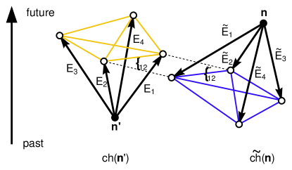
Necessary and sufficient conditions for constructing the triangulated manifold are obtained by considering the 4-simplexes of the pure complex. The complex is composed of two types of simplexes (which could be viewed as being local charts of an atlas), $ch(\mathbf{n})$ and $\widetilde{ch}(\mathbf{n})$,

$\displaystyle ch(\mathbf{n})=\{\mathbf{n},\mathbf{n}+\mu;\mu=1,\dots 4\}$ $\displaystyle\ \ \text{and}\ \ \ \widetilde{ch}(\mathbf{n})=\{\mathbf{n},\mathbf{n}-\mu;\mu=1,\dots 4\}\ .$ (44)

As schematically indicated in  Fig. 5, these simplexes are composed of an apex event and four causally related events on its forward or backward light cone respectively. We will refer to these special Minkowski simplexes with four light-like and six spatial edges as forward (backward) null-simplexes121212The corresponding 2-dimensional road atlas would be composed of charts that include just three cities, with one-way roads connecting a central city to the other two. The central city of any chart also is the central city of one other chart with reversed one-way roads (these two charts could be labeled past and future). In the universe every city is a central city on some chart. In the atlas of the duoverse peripheral cities (passive nodes) never are central ones on any chart. Every city is at the intersection of two one-way roads in both atlases..

Refer to caption
Figure 5: Color online. Schematic depiction of the elementary null-simplexes $ch(\mathbf{n}^{\prime})$ and $\widetilde{ch}(\mathbf{n})$ forming the simplicial complex of the duoverse with passive ($\circ$) and active ($\bullet$) nodes. In the universe all nodes are active. The four arrows of each simplex represent displacements to nodes on the forward ($ch(\mathbf{n}^{\prime})$) and backward ($\widetilde{ch}(\mathbf{n})$) light cone of the active nodes $\mathbf{n}^{\prime}$ and $\mathbf{n}$. They are specified by the forward and backward lat-frames $E_{\mu}(\mathbf{n}^{\prime})$ and $\widetilde{E}_{\mu}(\mathbf{n})$ respectively. These illuminate F- and B-tetrahedrons whose 6 spatial lengths are shown in yellow and blue. Dashed lines connect nodes that are to be identified in the pure simplicial complex. The corresponding common edge of the F-and B-tetrahedron has spatial length $\ell_{12}(\mathbf{n}-\Delta_{1}-\Delta_{2})=\widetilde{\ell}_{12}(\mathbf{n})$. This is the geometrical content of  Eq.(46). The four nodes $(\mathbf{n},\mathbf{n}-\Delta_{1},\mathbf{n}-\Delta_{2},\mathbf{n}=\mathbf{n}-\Delta_{1}-\Delta_{2}$ form a plaquette of the topologically hypercubic lattice with $\ell_{12}(\mathbf{n}-\Delta_{1}-\Delta_{2})=\widetilde{\ell}_{12}(\mathbf{n})$ on the diagonal. Note that the backward null lat-frames $\widetilde{E}_{\mu}$ are redundant (and not included as variables of the model): if the 6 spatial lengths $\widetilde{\ell}_{\mu\nu}$ of the B-tetrahedron satisfy the inequalities of  Eq.(V.1), the relative location of the apex $\mathbf{n}$ of the oriented backward null-simplex is uniquely determined.

Four of the faces of such a null-simplex of Minkowski space are tetrahedrons with 3 spatial and 3 null edges, the edges of the fifth (F- or B-) tetrahedron are all spatial. Any two of these simplexes (charts) have at most two events (and thus at most one length) in common. The non-trivial intersections of such simplexes are (with $\mu\neq\nu$),

$\displaystyle ch(\mathbf{n})$ $\displaystyle\cap ch(\mathbf{n}+\mu)$ $\displaystyle=$ $\displaystyle\{\mathbf{n}+\mu\}$
$\displaystyle ch(\mathbf{n})$ $\displaystyle\cap\widetilde{ch}(\mathbf{n}+\mu)$ $\displaystyle=$ $\displaystyle\{\mathbf{n},\mathbf{n}+\mu\},$ $\displaystyle\text{with }\ell^{2}_{\mu\mu}(\mathbf{n})=\widetilde{\ell}^{2}_{\mu\mu}(\mathbf{n}+\mu)=0$
$\displaystyle ch(\mathbf{n})$ $\displaystyle\cap ch(\mathbf{n}+\mu-\nu)$ $\displaystyle=$ $\displaystyle\{\mathbf{n}+\mu\}$
$\displaystyle ch(\mathbf{n})$ $\displaystyle\cap\widetilde{ch}(\mathbf{n})$ $\displaystyle=$ $\displaystyle\{\mathbf{n}\}$
$\displaystyle ch(\mathbf{n})$ $\displaystyle\cap\widetilde{ch}(\mathbf{n}+2\mu)$ $\displaystyle=$ $\displaystyle\{\mathbf{n}+\mu\}$
$\displaystyle ch(\mathbf{n})$ $\displaystyle\cap\widetilde{ch}(\mathbf{n}+\mu+\nu)$ $\displaystyle=$ $\displaystyle\{\mathbf{n}+\mu,\mathbf{n}+\nu\},$ $\displaystyle\text{with }\ell^{2}_{\mu\nu}(\mathbf{n})=\widetilde{\ell}^{2}_{\mu\nu}(\mathbf{n}+\mu+\nu)\ .$ (45)

Simplexes (charts) of the duoverse include a single active node ($\mathbf{n}$) and four passive ones.The first two intersections of  Eq.(V.1) can be ignored in this case because they do not occur in the simplicial complex of the duoverse (i.e. are not in the atlas).

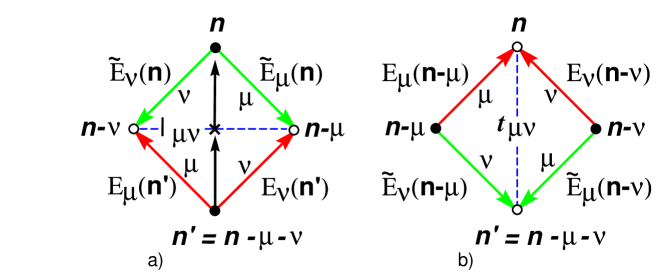
Introducing the backward null lat-frame $\{\widetilde{E}_{\mu}(\mathbf{n}),\mu=1,\dots,4\}$ on the backward light cone of an event $\mathbf{n}$ in the same manner as the forward null lat-frame $\{E_{\mu}(\mathbf{n}),\mu=1,\dots,4\}$ was defined on the forward light cone of $\mathbf{n}$, the simplexes (charts) can be consistently glued at their common overlap only if

$$\ell^{2}_{\mu\nu}(\mathbf{n}^{\prime}):=-2E_{\mu}(\mathbf{n}^{\prime})\cdot E_{\nu}(\mathbf{n}^{\prime})=-2\widetilde{E}_{\mu}(\mathbf{n})\cdot\widetilde{E}_{\nu}(\mathbf{n}):=\widetilde{\ell}^{2}_{\mu\nu}(\mathbf{n})\ ,\ \text{with }\mathbf{n}^{\prime}=\mathbf{n}-\mu-\nu\ \text{for all }\mu,\nu\ \text{ and }\mathbf{n}\ .$$ (46)

The same conclusion is reached by examining the typical $\mu\nu$-plaquette of the $\mathbf{\Lambda}$ lattice shown in  Fig. 6. If the lattice configuration is to represent a triangulated manifold, the events labeled by $\mathbf{n}-\mu$ and $\mathbf{n}-\nu$ need to be on the backward light cone of $\mathbf{n}$ and on the forward light cone of the event labeled by $\mathbf{n}^{\prime}=\mathbf{n}-\mu-\nu$. Note that $\mathbf{n}-\mu=\mathbf{n}^{\prime}+\nu$ and $\mathbf{n}-\nu=\mathbf{n}^{\prime}+\mu$ are the only nodes of the lattice in the intersection of these light cones.

Refer to caption
Figure 6: Color online. Constraints of a triangulated manifold. Plaquettes of $\mathbf{\Lambda}$ in the duoverse are of type a), with two spatially separate passive ($\circ$) nodes and two time-like separate active ($\bullet$) nodes or of type b), with two spatially separate active nodes and two time-like separate passive ones. Forward (backward) null lat-frames of the configuration are shown as red (green) arrows that point away from an active vertex and toward a passive one. In the universe all nodes are active. To construct a consistent simplicial complex, the spatial separation $\ell_{\mu\nu}$ between the events labeled by the nodes $\mathbf{n}-\mu$ and $\mathbf{n}-\nu$ must be the same for local inertial systems at $\mathbf{n}$ and $\mathbf{n}-\mu-\nu$. The time-like separation $t_{\mu\nu}$ between events represented by passive nodes $\mathbf{n}$ and $\mathbf{n}^{\prime}$ also is the same for local inertial systems at the active nodes $\mathbf{n}-\mu$ and $\mathbf{n}-\nu$. In a) the center-event of a plaquette at the midpoint of the spatial diagonal is marked by a cross ($\times$) and its time-like separation to the two active nodes indicated by solid (black) arrows (see  Sect.VII).

Including the case $\mu=\nu$,  Eq.(46) altogether imposes 10 independent $SL(2,\mathbb{C})\,$-invariant constraints per site on the backward lat-frames.

Equality of the time-like separation $t^{2}_{\mu\nu}$ between events $\mathbf{n}$ and $\mathbf{n}^{\prime}$ (see  Fig. 6b ) as viewed from inertial systems associated with $\mathbf{n}-\mu$ and $\mathbf{n}-\nu$ similarly requires that,

$$0=E_{\nu}(\mathbf{n}-\nu)\cdot\widetilde{E}_{\mu}(\mathbf{n}-\nu)-E_{\mu}(\mathbf{n}-\mu)\cdot\widetilde{E}_{\nu}(\mathbf{n}-\mu)\ \text{for all }\mu,\nu\ \text{ and }\mathbf{n}\ .$$ (47)

These are 6 additional independent linear constraints per site. The altogether 16 constraints per site of  Eq.(46) and  Eq.(47) offset the 16 degrees of freedom per site of the $\widetilde{E}$’s. No additional dynamical degrees of freedom have been introduced and one thus should be able to construct a TLT that constrains lattice configurations to those representing triangulated causal manifolds.

Eq.(46) as well as  Eq.(47) are invariant under local $SL(2,\mathbb{C})\,$transformations of all the lat-frames, but  Eq.(46) is invariant under independent $SL(2,\mathbb{C})\,$transformation of the backward and forward lat-frames at each active site. For a given configuration of forward null vectors $\{E_{\mu}(\mathbf{n});[\mathbf{n},\mu]\in\mathbf{\Lambda}\}$ the constraints (46) imply that,

$$\{0<\widetilde{\ell}_{\mu\nu}(\mathbf{n})=\ell^{2}_{\mu\nu}(\mathbf{n}-\mu-\nu)=-2E_{\mu}(\mathbf{n}-\mu-\nu)\cdot E_{\nu}(\mathbf{n}-\mu-\nu),\ \text{for }1\leq\mu<\nu\leq 4\}\ ,$$ (48)

are the spatial lengths of the 6 edges of a B-tetrahedron whose four vertices are on the backward light-cone of the event $\mathbf{n}$.

The six additional constraints of  Eq.(47) on the other hand apparently only serve to localize the additional $SL(2,\mathbb{C})\,$-invariance $\widetilde{E}_{\mu}(\mathbf{n})\rightarrow g(\mathbf{n})\widetilde{E}_{\mu}(\mathbf{n})g^{\dagger}(\mathbf{n})$ of the solution to  Eq.(46). The ten $SL(2,\mathbb{C})\,$-invariant constraints of  Eq.(46) in fact suffice to (uniquely) construct the whole complex. The geometry of this complex does not depend on the additional $SL(2,\mathbb{C})\,$degrees of freedom of the backward lat-frames.

As in the GPS Fang (1986); Abel and Chaffee (1991); Fang (1992), the apex $\mathbf{n}$ can be reconstructed from the vertices of the B-tetrahedron of $\widetilde{ch}(\mathbf{n})$. The discussion of light-cones in  Sect.IV implies that this is possible only if the 6 spatial lengths $\widetilde{\ell}_{\mu\nu}(\mathbf{n})=\ell_{\mu\nu}(\mathbf{n}-\mu-\nu)>0$ of  Eq.(48) satisfy the inequalities,

$\displaystyle\widetilde{\ell}_{12}(\mathbf{n})\widetilde{\ell}_{34}(\mathbf{n})$ $\displaystyle\leq\widetilde{\ell}_{13}(\mathbf{n})\widetilde{\ell}_{24}(\mathbf{n})+\widetilde{\ell}_{14}(\mathbf{n})\widetilde{\ell}_{23}(\mathbf{n})\ ,$
$\displaystyle\widetilde{\ell}_{13}(\mathbf{n})\widetilde{\ell}_{24}(\mathbf{n})$ $\displaystyle\leq\widetilde{\ell}_{12}(\mathbf{n})\widetilde{\ell}_{34}(\mathbf{n})+\widetilde{\ell}_{14}(\mathbf{n})\widetilde{\ell}_{23}(\mathbf{n})\ ,$
$\displaystyle\widetilde{\ell}_{14}(\mathbf{n})\widetilde{\ell}_{23}(\mathbf{n})$ $\displaystyle\leq\widetilde{\ell}_{12}(\mathbf{n})\widetilde{\ell}_{34}(\mathbf{n})+\widetilde{\ell}_{13}(\mathbf{n})\widetilde{\ell}_{24}(\mathbf{n})\ ,\ \text{for all}\ \mathbf{n}\ .$ (49)

Since all the lengths are positive, we again can combine the triangle inequalities of  Eq.(V.1) to the single requirement that,

$$\det{\widetilde{\ell}_{\mu\nu}(\mathbf{n})}\leq 0\ ,\ \text{for all}\ \mathbf{n}\ .$$ (50)

The inequalities of  Eq.(V.1) are $SL(2,\mathbb{C})\,$-invariant and select configurations of null lat-frames that represent triangulated causal manifolds. Due to  Eq.(50) the consistency conditions are the requirement that the 4-volume of every backward simplex $\widetilde{V}(\mathbf{n}):=\sqrt{-\det{\widetilde{\ell}^{2}_{\mu\nu}(\mathbf{n})}}$ be real.

These quasi-local but non-linear consistency conditions on the lattice configuration not only are reasonable and necessary but also are sufficient to reconstruct the oriented backward lat-frame up to $SL(2,\mathbb{C})\,$ transformation from the set of lengths $\{\widetilde{\ell}_{\mu\nu}(\mathbf{n})\}$ (see Appendix C). As outlined in  Sect.II, one then can reconstruct the simplicial complex of the triangulated manifold uniquely. The conditions of  Eq.(50) in some sense are ”integrability conditions” of the causal lattice.

V.2 The Manifold TLT

We here construct a local TLT whose partition function vanishes when  Eq.(V.1) is violated and is a (non-vanishing) constant otherwise. The TLT partition function evidently is proportional to the product of Heaviside functions that enforce the inequalities of Eq.(V.1). We wish to have a local integral representation of it. Many such representations exist. In Appendix D an equivariant BRST construction is used to obtain a local TLT in terms of the lat-frames that ensures  Eq.(46). Unfortunately this local TLT depends explicitly on the backward lat-frames and more than doubles the number of lattice variables. One also can simply enforce the single inequality of  Eq.(50), which is of rather high order in the lattice variables.

Here we construct a simpler TLT based on the spinor formulation of the lattice model. It requires just two new variables (spinor phases) per site to enforce  Eq.(V.1) with a local lattice action of the same scaling dimension as the cosmological term.

Consider therefore the representation of backward null lat-frames $\widetilde{E}_{\mu}^{A\dot{B}}(\mathbf{n})$ by spinors $\widetilde{\xi}^{A}_{\mu}(\mathbf{n})$,

$$\widetilde{E}_{\mu}^{AB^{\prime}}(\mathbf{n})=-i(\widetilde{\xi}_{\mu}\otimes\widetilde{\xi}^{*}_{\mu})^{AB^{\prime}}=-i\widetilde{\xi}_{\mu}^{A}(\mathbf{n})\widetilde{\xi}^{*B^{\prime}}_{\mu}(\mathbf{n})\ .$$ (51)

The only difference to representation of forward lat-frames by spinors in Eq.(25) is the minus sign in  Eq.(51). It implies that $-i{\rm Tr}\widetilde{E}_{\mu}(\mathbf{n})=-(|\widetilde{\xi}_{\mu}^{1}(\mathbf{n})|^{2}+|\widetilde{\xi}_{\mu}^{2}(\mathbf{n})|^{2})<0$. $\widetilde{E}_{\mu}(\mathbf{n})$ thus is on the backward light cone.

Events labeled by $\mathbf{n}-\mu$ and $\mathbf{n}-\nu$ are spatially separated by,

$$\widetilde{\ell}_{\mu\nu}(\mathbf{n})=|\widetilde{\xi}^{A}_{\mu}(\mathbf{n})\varepsilon_{AB}\widetilde{\xi}^{B}_{\nu}(\mathbf{n})|\ ,$$ (52)

and  Eq.(46) demands that,

$$\widetilde{\ell}^{2}_{\mu\nu}(\mathbf{n})=\ell^{2}_{\mu\nu}(\mathbf{n}-\mu-\nu)=|f_{\mu\nu}(\mathbf{n}-\mu-\nu)|^{2}\ .$$ (53)

A configuration of forward spinors $\{\xi_{\mu}(\mathbf{n})\}$ thus is compatible with a triangulated manifold only if real phases $\varphi_{\mu\nu}(\mathbf{n})=\varphi_{\nu\mu}(\mathbf{n})$ and backward spinors $\widetilde{\xi}_{\mu}(\mathbf{n})$ exist for which,

$$\widetilde{\xi}^{A}_{\mu}(\mathbf{n})\varepsilon_{AB}\widetilde{\xi}^{B}_{\nu}(\mathbf{n})=\widetilde{f}_{\mu\nu}(\mathbf{n}):=e^{i\varphi_{\mu\nu}(\mathbf{n})}f_{\mu\nu}(\mathbf{n}-\mu-\nu)\ \text{for all }\mathbf{n},\mu,\nu\ .$$ (54)

The skew-symmetric matrix $\widetilde{f}_{\mu\nu}(\mathbf{n})$ defined by the right-hand-side of  Eq.(54) is described by spinors only if its Pfaffian vanishes131313If $\text{Pf}[\widetilde{f}(\mathbf{n})]=0$, $\widetilde{f}_{\mu\nu}(\mathbf{n})=\gamma(X_{\mu}Y_{\nu}-X_{\nu}Y_{\mu})$ where the two linearly independent vectors $X_{\mu}$ and $Y_{\mu}$ span the two-dimensional kernel of the dual tensor $\widetilde{f}^{\mu\nu}=\sum_{\rho,\sigma}{\textstyle\frac{1}{2}}\varepsilon(\mu\nu\rho\sigma)\widetilde{f}_{\rho\sigma}(\mathbf{n})$ and $\gamma$ is a complex number. A possible set of spinors then is $\widetilde{\xi}_{\mu}(\mathbf{n})=(\gamma X_{\mu},Y_{\mu})$.. A configuration therefore represents a triangulated manifold only if a set of phases $\{\varphi_{\mu\nu}(\mathbf{n})=\varphi_{\nu\mu}(\mathbf{n})\in\mathbb{R}\}$ exists for which

$$0=\text{Pf}(\widetilde{f}(\mathbf{n}))=\widetilde{f}_{12}(\mathbf{n})\widetilde{f}_{34}(\mathbf{n})+\widetilde{f}_{13}(\mathbf{n})\widetilde{f}_{42}(\mathbf{n})+\widetilde{f}_{14}(\mathbf{n})\widetilde{f}_{23}(\mathbf{n})\ \text{for all}\ \mathbf{n}\ ,$$ (55)

where $\widetilde{f}_{\mu\nu}(\mathbf{n})$ is given by  Eq.(54). Note that this formulation of the consistency condition assures the existence of backward spinors $\widetilde{\xi}_{\mu}(\mathbf{n})$ without explicitly constructing them.

The phases $\{\varphi_{\mu\nu}(\mathbf{n})\}$ can be found and  Eq.(55) satisfied only if the magnitudes of the three complex numbers,

$\displaystyle\widetilde{a}(\mathbf{n})$ $\displaystyle:=|f_{12}(\mathbf{n}-\mathbf{\Delta}_{1}-\mathbf{\Delta}_{2})f_{34}(\mathbf{n}-\mathbf{\Delta}_{3}-\mathbf{\Delta}_{4})|=\widetilde{\ell}_{12}(\mathbf{n})\widetilde{\ell}_{34}(\mathbf{n})$
$\displaystyle\widetilde{b}(\mathbf{n})$ $\displaystyle:=|f_{13}(\mathbf{n}-\mathbf{\Delta}_{1}-\mathbf{\Delta}_{3})f_{42}(\mathbf{n}-\mathbf{\Delta}_{2}-\mathbf{\Delta}_{4})|=\widetilde{\ell}_{13}(\mathbf{n})\widetilde{\ell}_{24}(\mathbf{n})$
$\displaystyle\widetilde{c}(\mathbf{n})$ $\displaystyle:=|f_{14}(\mathbf{n}-\mathbf{\Delta}_{1}-\mathbf{\Delta}_{4})f_{23}(\mathbf{n}-\mathbf{\Delta}_{2}-\mathbf{\Delta}_{3})|=\widetilde{\ell}_{14}(\mathbf{n})\widetilde{\ell}_{23}(\mathbf{n})\ ,$ (56)

form the sides of a triangle. To construct the pure simplicial complex of a triangulated causal manifold, the spatial lengths $\widetilde{\ell}_{\mu\nu}(\mathbf{n})=|f_{\mu\nu}(\mathbf{n}-\mathbf{\Delta}_{\mu}-\mathbf{\Delta}_{\nu})|=\ell_{\mu\nu}(\mathbf{n}-\mathbf{\Delta}_{\mu}-\mathbf{\Delta}_{\nu})$ thus must satisfy the inequalities of  Eq.(V.1).

Suppose that for a configuration of forward spinors a set of phases $\varphi_{\mu\nu}$ can be found for which  Eq.(55) is satisfied. We first demonstrate that a physically equivalent configuration of forward spinors exists in this case that satisfies  Eq.(55) with vanishing phases.

The $U^{4}(1)$ invariance of physical observables (and lat-frames) of  Eq.(28) implies the equivalence of phases,

$$\varphi_{\mu\nu}(\mathbf{n})\equiv\varphi^{\prime}_{\mu\nu}(\mathbf{n})=\varphi_{\mu\nu}(\mathbf{n})-\psi_{\mu}(\mathbf{n}-\mu-\nu)-\psi_{\nu}(\mathbf{n}-\mu-\nu)\ .$$ (57)

For $\text{Pf}[\widetilde{f}(\mathbf{n})]=0$ the overall phase is irrelevant and we need only construct a representative set of spinors for which the phases of the three terms of the Pfaffian coincide, that is

$$\varphi^{\prime}_{12}(\mathbf{n})+\varphi^{\prime}_{34}(\mathbf{n})=\varphi^{\prime}_{13}(\mathbf{n})+\varphi^{\prime}_{42}(\mathbf{n})=\varphi^{\prime}_{14}(\mathbf{n})+\varphi^{\prime}_{23}(\mathbf{n})\ .$$ (58)

Given the initial set of phases $\{\varphi_{\mu\nu}(\mathbf{n})\}$ for which  Eq.(55) is satisfied, the $2N$ linear constraints of  Eq.(58) on the $4N$ phases $\psi_{\mu}(\mathbf{n})$ in general allow for an infinite set of solutions. To have a more manageable set we restrict to $\psi_{1}(\mathbf{n})=-\psi_{2}(\mathbf{n})$ and $\psi_{3}(\mathbf{n})=-\psi_{4}(\mathbf{n})$. Defining $\psi_{\pm}(\mathbf{n}):=\psi_{1}(\mathbf{n})\pm\psi_{3}(\mathbf{n})=-\psi_{2}(\mathbf{n})\mp\psi_{4}(\mathbf{n})$, the conditions of  Eq.(58) then decouple into two equations,

$\displaystyle\psi_{+}(\mathbf{n}-\mathbf{\Delta}_{2}-\mathbf{\Delta}_{4})-\psi_{+}(\mathbf{n}-\mathbf{\Delta}_{1}-\mathbf{\Delta}_{3})$ $\displaystyle=\varphi_{12}(\mathbf{n})+\varphi_{34}(\mathbf{n})-\varphi_{13}(\mathbf{n})-\varphi_{24}(\mathbf{n})\hskip 30.00005pt\mod{2\pi}$
$\displaystyle\psi_{-}(\mathbf{n}-\mathbf{\Delta}_{2}-\mathbf{\Delta}_{3})-\psi_{-}(\mathbf{n}-\mathbf{\Delta}_{1}-\mathbf{\Delta}_{4})$ $\displaystyle=\varphi_{12}(\mathbf{n})+\varphi_{34}(\mathbf{n})-\varphi_{14}(\mathbf{n})-\varphi_{23}(\mathbf{n})\hskip 30.00005pt\mod{2\pi}\ ,$ (59)

that relate the $\psi_{\pm}$ angles at the endpoints of two diagonals of a hypercube. With appropriate boundary conditions  Eq.(V.2) uniquely determines the angles $\psi_{\pm}(\mathbf{n}),\mod{2\pi}$. The angles $\psi_{1}(\mathbf{n})=(\psi_{+}(\mathbf{n})+\psi_{-}(\mathbf{n}))/2$ and $\psi_{2}(\mathbf{n})=(\psi_{+}(\mathbf{n})-\psi_{-}(\mathbf{n}))/2$ then are known modulo $\pi$ and the new spinors $\{\xi^{\prime}_{\mu}(\mathbf{n}),\mu=1,\dots,4\}$ are determined up to sign.

Let us therefore attempt to construct the TLT that enforces the manifold condition by imposing $\text{Pf}[\widetilde{f}(\mathbf{n})]=0$ at all nodes $\mathbf{n}$ as a $U^{2}(1)$ gauge condition on the spinors. This ”gauge” conditions has a solution only if the corresponding configuration of forward null lat-frames represents a triangulated manifold141414The forward null lat-frames do not depend on the spinor phases and are $U^{4}(1)$ invariants..

We introduce ghosts $c_{\pm}$ and a corresponding BRST-doublet of complex anti-ghosts $\bar{c},\bar{c}^{*}$ as well as complex Lagrange multiplier fields $\eta,\eta^{*}$. The nilpotent BRST-variation of the spinor phases $\psi_{\pm}$ and of these additional fields is,

$\displaystyle s\psi_{\pm}(\mathbf{n})$ $\displaystyle=c_{\pm}(\mathbf{n}),\ sc_{\pm}(\mathbf{n})=0$ $\displaystyle s\bar{c}(\mathbf{n})$ $\displaystyle=\eta(\mathbf{n}),\ s\eta(\mathbf{n})=0$ $\displaystyle s\bar{c}^{*}(\mathbf{n})$ $\displaystyle=\eta^{*}(\mathbf{n}),\ s\eta^{*}(\mathbf{n})=0\ ,$ (60)

with a trivial extension to other fields. We therefore consider the TLT with the BRST-exact Lagrangian,

$\displaystyle\mathcal{L}_{TLT}(\mathbf{n})$ $\displaystyle=s[\bar{c}^{*}(\mathbf{n})\text{Pf}[f^{\prime}(\mathbf{n})]+\bar{c}(\mathbf{n})\text{Pf}[f^{\prime*}(\mathbf{n})]+i\frac{\alpha}{2}(\eta^{*}(\mathbf{n})\bar{c}(\mathbf{n})+\eta(\mathbf{n})\bar{c}^{*}(\mathbf{n}))]$
$\displaystyle=\eta^{*}(\mathbf{n})\text{Pf}[f^{\prime}(\mathbf{n})]+\eta(\mathbf{n})\text{Pf}[f^{\prime}(\mathbf{n})]+i\alpha\eta(\mathbf{n})\eta^{*}(\mathbf{n})+$ (61)
$\displaystyle\hskip 30.00005pt+i\left(\begin{matrix}\bar{c}(\mathbf{n})&\bar{c}^{*}(\mathbf{n})\end{matrix}\right)\cdot\left(\begin{matrix}f^{\prime*}_{13}(\mathbf{n})f^{\prime*}_{42}(\mathbf{n})&f^{\prime*}_{14}(\mathbf{n})f^{\prime*}_{32}(\mathbf{n})\\ f^{\prime}_{13}(\mathbf{n})f^{\prime}_{42}(\mathbf{n})&f^{\prime}_{14}(\mathbf{n})f^{\prime}_{32}(\mathbf{n})\end{matrix}\right)\cdot\left(\begin{matrix}c_{+}(\mathbf{n}-\mathbf{\Delta}_{1}-\mathbf{\Delta}_{3})-c_{+}(\mathbf{n}-\mathbf{\Delta}_{2}-\mathbf{\Delta}_{4})\\ c_{-}(\mathbf{n}-\mathbf{\Delta}_{1}-\mathbf{\Delta}_{4})-c_{-}(\mathbf{n}-\mathbf{\Delta}_{2}-\mathbf{\Delta}_{3})\end{matrix}\right)\ ,$

where we have introduced a gauge-parameter $\alpha\geq 0$. $f^{\prime}(\mathbf{n})$ in  Eq.(V.2) depends on the spinorial phases and is the skew-symmetric matrix with components,

$\displaystyle f^{\prime}_{12}(\mathbf{n})$ $\displaystyle=-f^{\prime}_{21}(\mathbf{n}):=f_{12}(\mathbf{n}-\mathbf{\Delta}_{1}-\mathbf{\Delta}_{2})$
$\displaystyle f^{\prime}_{34}(\mathbf{n})$ $\displaystyle=-f^{\prime}_{43}(\mathbf{n}):=f_{34}(\mathbf{n}-\mathbf{\Delta}_{3}-\mathbf{\Delta}_{4})$
$\displaystyle f^{\prime}_{13}(\mathbf{n})$ $\displaystyle=-f^{\prime}_{31}(\mathbf{n}):=e^{-i\psi_{+}(\mathbf{n}-\mathbf{\Delta}_{1}-\mathbf{\Delta}_{3})}f_{13}(\mathbf{n}-\mathbf{\Delta}_{1}-\mathbf{\Delta}_{3})$
$\displaystyle f^{\prime}_{24}(\mathbf{n})$ $\displaystyle=-f^{\prime}_{42}(\mathbf{n}):=e^{+i\psi_{+}(\mathbf{n}-\mathbf{\Delta}_{2}-\mathbf{\Delta}_{4})}f_{24}(\mathbf{n}-\mathbf{\Delta}_{2}-\mathbf{\Delta}_{4})$
$\displaystyle f^{\prime}_{14}(\mathbf{n})$ $\displaystyle=-f^{\prime}_{41}(\mathbf{n}):=e^{-i\psi_{-}(\mathbf{n}-\mathbf{\Delta}_{1}-\mathbf{\Delta}_{4})}f_{14}(\mathbf{n}-\mathbf{\Delta}_{1}-\mathbf{\Delta}_{4})$
$\displaystyle f^{\prime}_{23}(\mathbf{n})$ $\displaystyle=-f^{\prime}_{32}(\mathbf{n}):=e^{+i\psi_{-}(\mathbf{n}-\mathbf{\Delta}_{2}-\mathbf{\Delta}_{3})}f_{23}(\mathbf{n}-\mathbf{\Delta}_{2}-\mathbf{\Delta}_{3})\ .$ (62)

The partition function of this TLT is,

$\displaystyle Z^{TLT}_{\alpha}[\xi]$ $\displaystyle\propto\prod_{\mathbf{n}}\int dc_{+}(\mathbf{n})dc_{-}(\mathbf{n})d\bar{c}(\mathbf{n})d\bar{c}^{*}(\mathbf{n})\int_{S_{1}\times S_{1}}d\psi_{+}(\mathbf{n})d\psi_{-}(\mathbf{n})\int_{\mathbb{R}^{2}}d\eta(\mathbf{n})d\eta^{*}(\mathbf{n})e^{i\mathcal{L}_{TLT}(\mathbf{n})}$
$\displaystyle\propto\prod_{\mathbf{n}}\int_{S_{1}\times S_{1}}d\psi_{+}(\mathbf{n})d\psi_{-}(\mathbf{n})\widetilde{V}(\mathbf{n})\;e^{-\frac{1}{\alpha}\left|\text{Pf}[f^{\prime}(\mathbf{n})]\right|^{2}}\ .$ (63)

The last expression is obtained by integrating over ghost and Lagrange multiplier fields and

$$\widetilde{V}(\mathbf{n}):={\textstyle\frac{1}{2}}\text{Im}f^{\prime}_{13}(\mathbf{n})f^{\prime*}_{32}(\mathbf{n})f^{\prime}_{24}(\mathbf{n})f^{\prime*}_{41}(\mathbf{n})={\textstyle{\frac{i}{4}}}\det{\left(\begin{matrix}f^{\prime*}_{13}(\mathbf{n})f^{\prime*}_{42}(\mathbf{n})&f^{\prime*}_{14}(\mathbf{n})f^{\prime*}_{32}(\mathbf{n})\\ f^{\prime}_{13}(\mathbf{n})f^{\prime}_{42}(\mathbf{n})&f^{\prime}_{14}(\mathbf{n})f^{\prime}_{32}(\mathbf{n})\end{matrix}\right)}\ .$$ (64)

In the limit $\alpha\rightarrow 0^{+}$, only spinor configurations that satisfy $\text{Pf}[f^{\prime}(\mathbf{n})]\sim 0$ contribute significantly to the integral of  Eq.(V.2). This is the condition we wish to enforce, but one can show Witten (1988b); Baulieu and Schaden (1998); Schaden (1999) that151515Viewing $\text{Pf}[f^{\prime}(.)]$ as a smooth 2N-dimensional real vector field on $T_{2N}=(S_{1}\times S_{1})^{N}$ with coordinates $(\psi_{+}(.),\psi_{-}(.))$, this is a consequence of the Poincaré-Hopf theoremBirmingham et al. (1991). $Z^{TLT}_{\alpha}[\xi]$ is proportional to the Euler characteristic of the 2N-dimensional torus $T_{2N}=(S_{1}\times S_{1})^{N}$. As defined in  Eq.(V.2) $Z^{TLT}_{\alpha}[\xi]$ therefore vanishesNeuberger (1987); Schaden (1999) for any $\alpha>0$ and spinor configuration $\{\xi\}$. This TLT thus fails to constrain to configurations that satisfy the consistency condition.

Fortunately this can be rectified. We already know that any skew-symmetric complex matrix with vanishing Pfaffian may be written in terms of spinors. Configurations that contribute significantly to the integral of  Eq.(V.2) in the limit $\alpha\rightarrow 0^{+}$ thus can be written in terms of backward spinors as,

$$f^{\prime}_{\mu\nu}(\mathbf{n})=\widetilde{\xi}^{A}_{\mu}(\mathbf{n})\varepsilon_{AB}\widetilde{\xi}^{B}_{\nu}(\mathbf{n})\ .$$ (65)

For $\text{Pf}[f^{\prime}(\mathbf{n})]=0$, $\widetilde{V}(\mathbf{n})$, given by  Eq.(64), therefore is just the (signed) four dimensional volume element,

$$\widetilde{V}(\mathbf{n})=-\textstyle{\frac{i}{2}}{\rm Tr}\widetilde{E}_{3}(\mathbf{n})\varepsilon\widetilde{E}^{T}_{2}(\mathbf{n})\varepsilon\widetilde{E}_{4}(\mathbf{n})\varepsilon\widetilde{E}_{1}^{T}(\mathbf{n})=\det[\widetilde{E}(\mathbf{n})]\ ,$$ (66)

of the backward null lat-frames given by Eq.(51). The lengths $\widetilde{\ell}_{\mu\nu}(\mathbf{n})=|f^{\prime}_{\mu\nu}(\mathbf{n})|$ themselves do not depend on spinor phases. Positive and negative contributions to $Z^{TLT}_{0^{+}}[\xi]$ in  Eq.(V.2) thus arise from different signs of the 4-volumes $\widetilde{V}(\mathbf{n})$ of configurations with the same set of spatial lengths $\{\widetilde{\ell}_{\mu\nu}(\mathbf{n})\}$. Non-singular solutions to $\text{Pf}[f^{\prime}(\mathbf{n})]=0$ in fact come in pairs with $\widetilde{V}(\mathbf{n})$ of opposite sign and this leads to $Z^{TLT}_{0^{+}}[\xi]=0$.

Orientable manifolds on the other hand ought to be triangulated by spinor configurations for which $\widetilde{V}(\mathbf{n})>0$ at all sites $\mathbf{n}$. It thus is tempting to modify the TLT to,

$$\widetilde{Z}^{TLT}[\xi]=\lim_{\alpha\rightarrow 0^{+}}\prod_{\mathbf{n}}\alpha^{-1}\int_{S_{1}\times S_{1}}d\psi_{+}(\mathbf{n})d\psi_{-}(\mathbf{n})\widetilde{V}(\mathbf{n})\Theta[\widetilde{V}(\mathbf{n})]\;e^{-\frac{1}{\alpha}\left|\text{Pf}[f^{\prime}(\mathbf{n})]\right|^{2}}\ ,$$ (67)

where $\Theta[x]$ is the Heaviside distribution. The question arises whether $\widetilde{Z}^{TLT}$ is a topological integral that does not depend on generic variations of the spinor configuration. This generally will not be true if the number of (pairs of) solutions depends on the configuration.

We can assure ourselves that this is not the case by explicit evaluation of  Eq.(67). Note that $\widetilde{V}(\mathbf{n})$, defined in  Eq.(64), depends on the following differences of the angles in  Eq.(V.2) only,

$\displaystyle\theta(\mathbf{n})$ $\displaystyle={\textstyle\frac{1}{2}}(\Psi_{+}(\mathbf{n}-\mathbf{\Delta}_{2}-\mathbf{\Delta}_{4})-\Psi_{+}(\mathbf{n}-\mathbf{\Delta}_{1}-\mathbf{\Delta}_{3})+\Psi_{-}(\mathbf{n}-\mathbf{\Delta}_{2}-\mathbf{\Delta}_{3})-\Psi_{-}(\mathbf{n}-\mathbf{\Delta}_{1}-\mathbf{\Delta}_{4}))$
$\displaystyle\varphi(\mathbf{n})$ $\displaystyle=\Psi_{+}(\mathbf{n}-\mathbf{\Delta}_{2}-\mathbf{\Delta}_{4})-\Psi_{+}(\mathbf{n}-\mathbf{\Delta}_{1}-\mathbf{\Delta}_{3})-\Psi_{-}(\mathbf{n}-\mathbf{\Delta}_{2}-\mathbf{\Delta}_{3})+\Psi_{-}(\mathbf{n}-\mathbf{\Delta}_{1}-\mathbf{\Delta}_{4})\ .$ (68)

The partition function of  Eq.(67) thus factorizes in the form,

$$\widetilde{Z}^{TLT}[\xi]=\prod_{\mathbf{n}}\Upsilon[f_{12}(\mathbf{n}-\mathbf{\Delta}_{1}-\mathbf{\Delta}_{2})f_{34}(\mathbf{n}-\mathbf{\Delta}_{3}-\mathbf{\Delta}_{4}),f_{13}(\mathbf{n}-\mathbf{\Delta}_{1}-\mathbf{\Delta}_{3})f_{42}(\mathbf{n}-\mathbf{\Delta}_{2}-\mathbf{\Delta}_{4}),f_{14}(\mathbf{n}-\mathbf{\Delta}_{1}-\mathbf{\Delta}_{4})f_{23}(\mathbf{n}-\mathbf{\Delta}_{2}-\mathbf{\Delta}_{3})]\ ,$$ (69)

with,

$$\Upsilon[a,b,c]:=\lim_{\alpha\rightarrow 0^{+}}\frac{1}{\pi\alpha}\int_{0}^{2\pi}d\theta\int_{0}^{2\pi}d\varphi\ \text{Im}(bc^{*}e^{i\varphi})\Theta[\text{Im}(bc^{*}e^{i\varphi})]\exp\left\{-\frac{1}{\alpha}\left|a+b\;e^{i(\theta+\varphi/2)}+c\;e^{i(\theta-\varphi/2)}\right|^{2}\right\}\ .$$ (70)

For $\alpha\rightarrow 0^{+}$ the two-dimensional integral of  Eq.(70) may be evaluated semiclassically. The exponent vanishes only at (absolute) extrema that satisfy the triangle inequalities,

$$|a|\leq|b|+|c|\ \wedge\ |b|\leq|c|+|a|\ \wedge\ |c|\leq|a|+|b|\ ,$$ (71)

If  Eq.(71) holds, these extrema correspond to angles $\bar{\theta},\bar{\varphi}$ that satisfy,

$$|a|^{2}=|b|^{2}+|c|^{2}+2\text{Re}\;bc^{*}e^{i\bar{\varphi}}\ ,\ e^{2i\bar{\theta}}=\frac{a(b^{*}e^{-i\bar{\varphi}/2}+c^{*}e^{i\bar{\varphi}/2})}{a^{*}(be^{i\bar{\varphi}/2}+ce^{-i\bar{\varphi}/2})}\ .$$ (72)

As  Fig. 7 illustrates, the exponent generically vanishes at pairs of absolute minima161616If $a$ is taken to be real, the two extrema correspond to letting $(b,c)\rightarrow(b^{*},c^{*})$., with angles $\bar{\varphi}$ and $\bar{\varphi}^{\prime}$ related by $bc^{*}e^{i\bar{\varphi}}=b^{*}c\,e^{-i\bar{\varphi}^{\prime}}$. Both extrema satisfy  Eq.(72), but give the opposite sign for $\widetilde{V}(\mathbf{n})=\text{Im}\;bc^{*}e^{i\bar{\varphi}}$.

Refer to caption
Figure 7: The pair of generic extrema with $a+b+c=0$ for given magnitudes of the complex numbers $b$ and $c$. The magnitudes $|a|,|b|,|c|$ satisfy the triangle inequalities of  Eq.(71). Both solutions coincide only if $|a|=||b|\pm|c||$.

The Gaussian integral over fluctuations around these absolute minima furthermore are the same and proportional to $\alpha/|\text{Im }bc^{*}e^{i\bar{\varphi}}|$ The total contribution to the partition function for $\alpha\rightarrow 0^{+}$ thus gives the vanishing Euler characteristic of the 2-torus if one sums over both minima. Taking only solutions with positive volume in Eq.(70) on the other hand leads to a non-vanishing partition function that generically does not depend on $a,b$ and $c$ as long as these satisfy the inequalities of  Eq.(71). $\Upsilon[a,b,c]$ on the other hand vanishes exponentially in the limit $\alpha\rightarrow 0+$ when  Eq.(71) is violated. $\Upsilon[a,b,c]$ thus is an integral representation of the distribution,

$$\Upsilon(a,b,c)=\Theta(|a|+|b|-|c|)\ \Theta(|b|+|c|-|a|)\ \Theta(|c|+|a|-|b|)=\Theta(2a^{2}b^{2}+2b^{2}c^{2}+2c^{2}a^{2}-a^{4}-b^{4}-c^{4})\ ,$$ (73)

Where $\Theta(x)$ is the Heaviside function. It is a constant if $a,b,c$ satisfy triangle inequalities and vanishes otherwise.

The TLT partition function of  Eq.(67) thus constrains the space of configurations to those satisfying  Eq.(V.1) that correspond to triangulated causal manifolds. Note that $\widetilde{Z}^{TLT}$ is a topological lattice integral in the limit $\alpha\rightarrow 0^{+}$ only. For $\alpha>0$, the integral does depend on the configuration. However, the limit $\alpha\rightarrow 0^{+}$ appears to be smooth and well-defined for $|a|^{2}>\alpha$. Regularization of the model in  Sect.VIII.3 ensures that this bound is satisfied.

VI Partial Localization to an $SU(2)$-structure group

The action of Eq.(41) is real and the weight $e^{iS_{\text{HP}}}$ of a configuration therefore oscillatory. Although $S_{\text{HP}}$ is unbounded, it is conceivable that configurations with very large classical action do not contribute to the integral, as in ordinary Fresnel integrals.

Even if this is the case, the Lorentzian model with the lattice action of  Eq.(41) is not well defined because its $SL(2,\mathbb{C})\,$structure group is not compact. The infinite volume of this group formally cancels in the expectation value of invariant physical observables, but it prevents one from defining a finite generating function even for a lattice with a finite number of sites. Contrary to ordinary lattice gauge theories with compact structure group, the $SL(2,\mathbb{C})\,$structure group of this model has to be localized to a compact subgroup for the generating function to be defined. The localization to an $SU(2)$-invariant lattice theory (where only the subgroup of local spatial rotations remains free) in fact is unique. The following partial gauge fixing of lattice configurations in this sense does not suffer of a Gribov Gribov (1978); Singer (1978) ambiguity.

Consider the local $SU(2)$-invariant Morse function constructed from the spinors of a single active node $\mathbf{n}$,

$$W_{\xi}[g(\mathbf{n})]=\sum_{\mu}w_{\mu}(\mathbf{n})\xi^{\dagger}_{\mu}(\mathbf{n})g^{\dagger}(\mathbf{n})g(\mathbf{n})\xi_{\mu}(\mathbf{n})=\sum_{\mu}w_{\mu}(\mathbf{n})\tau^{(g)}_{\mu}(\mathbf{n})\ ,$$ (74)

where $\{w_{\mu}(\mathbf{n})\}$ is a set of non-negative weights. This Morse function is proportional to an average over the positive time components $\tau^{(g)}_{\mu}=-i{\textstyle\frac{1}{2}}{\rm Tr}g(\mathbf{n})E_{\mu}(\mathbf{n})g^{\dagger}(\mathbf{n})$ of the $SL(2,\mathbb{C})\,$-transformed null lat-frame. It is bounded below and invariant under the $SU(2)$ subgroup of spatial rotations. Considered as a function of $g(\mathbf{n})\in\textrm{$SL(2,\mathbb{C})\,$}$ for a given spinor configuration, $W_{\xi}[g(\mathbf{n})]$ thus is a function on the coset space $\textrm{$SL(2,\mathbb{C})\,$}/SU(2)$ only. Decomposing $g\in\textrm{$SL(2,\mathbb{C})\,$}$ into a hermitian and a unitary part, both of unit determinant,

$$g=uh,\text{with }h=h^{\dagger}=e^{-i\vec{v}\cdot\vec{\sigma}},\ \text{and }u\in SU(2)\ ,$$ (75)

critical points of $W_{\xi}$ are characterized by,

$$0=-i\sum_{\mu}w_{\mu}(\mathbf{n})\xi^{\dagger}_{\mu}(\mathbf{n})\,\vec{\sigma}\,\xi_{\mu}(\mathbf{n})\ .$$ (76)

The $3\times 3$ Hessian matrix $H$ of this Morse function is strictly positive and proportional to the identity,

$$H(\mathbf{n})={\mathbb{1}}\sum_{\mu}w_{\mu}(\mathbf{n})\tau^{(g)}_{\mu}(\mathbf{n})={\mathbb{1}}W_{\xi}[g(\mathbf{n})]\ .$$ (77)

$\det[H(\mathbf{n})]$ vanishes only if $W_{\xi}[g(\mathbf{n})]=0$, that is, when the null lat-frame is singular171717The invariant regularization of the theory in  Sect.VIII.3 implies that $\det{E(\mathbf{n})}:=\det{(E^{a}_{\mu}(\mathbf{n}))}>0$ for all $\mathbf{n}$.. The non-trivial solution to  Eq.(76) thus is unique (modulo spatial $SU(2)$ rotations) and the Euler characteristic $\chi(\textrm{$SL(2,\mathbb{C})\,$}/SU(2))=\chi(H_{3})=1$. Note that this partial gauge eliminates one of the Lorentz components of a forward null lat-frame as a dynamical variable.

Several partial localizations of this kind are of special interest. They differ only in the choice of weights $w_{\mu}(\mathbf{n})\geq 0$ in  Eq.(74).

  • The most practical partial localization uses just two linearly independentfootnotemark: null vectors at each node. Setting $w_{1}(\mathbf{n})=w_{2}(\mathbf{n})=0$ and $w_{3}(\mathbf{n})=w_{4}(\mathbf{n})>0$, the gauge condition of  Eq.(76) implies that $\vec{E}_{4}(\mathbf{n})=-\vec{E}_{3}(\mathbf{n})$ and $\tau_{3}(\mathbf{n})=\tau_{4}(\mathbf{n})=|\vec{E}_{3}(\mathbf{n})|$, i.e. the corresponding two events appear simultaneous in this local inertial system. A spinorial solution to this condition is,

    $$\xi_{4}^{1}(\mathbf{n})=-\xi_{3}^{2*}(\mathbf{n}),\ \ \ \xi_{4}^{2}(\mathbf{n})=\xi_{3}^{1*}(\mathbf{n})\ .$$ (78)

    It is unique up to $U(1)$ phase transformations of the spinors. Note that  Eq.(78) is compatible with the choice made in  Sect.V to solve the consistency constraints with $\psi_{3}(\mathbf{n})=-\psi_{4}(\mathbf{n})$. Due to its simplicity, the partial localization of  Eq.(78) will be used in much of the following.

  • It may be desirable to choose equal weights for three of the four components, i.e. $w_{4}(\mathbf{n})=0$ and $w_{1}(\mathbf{n})=w_{2}(\mathbf{n})=w_{3}(\mathbf{n})>0$. The spatial components of three null vectors here form a triangle whose side-lengths are the temporal components of these null vectors. However, an explicit solution to  Eq.(76) in terms of the spinors is quite involved.

  • Sometimes a more equitable gauge condition is preferable that weights all components equally $w_{1}(\mathbf{n})=w_{2}(\mathbf{n})=w_{3}(\mathbf{n})=w_{4}(\mathbf{n})$ .  Eq.(76) then implies that the spatial parts of the four null-vectors of the lat-frame sum to zero. This gauge condition is used to reconstruct the backward lat-frame in Appendix C.

  • The weights $w_{\mu}(\mathbf{n})$ in  Eq.(74) can be any positive $SL(2,\mathbb{C})\,$-invariants of the fields. A judicious choice of these invariants may sometimes be advantageous (as ’t Hooft gauges are in spontaneously broken gauge theories). In the next section we have occasion to consider path-dependent gauges where the weights $w_{\mu}(\mathbf{n})$ depend on $\mathbf{n}$ in a manner that simplifies the computation of a path-dependent quantity, such as the proper time.

The partial localization of $SL(2,\mathbb{C})\,$to the SU(2) subgroup at each site of the lattice may also be achieved by an equivariant BRST construction Birmingham et al. (1991); Schaden (1999). Since the gauge condition here is ultra-local, the construction here is rather trivial, but it illustrates the general principle. The nilpotent BRST variation of the spinors, ghosts ($\vec{c}$ and $\vec{\omega}$) and auxiliary fields ($\vec{b}$ and $\vec{\bar{c}}$) is,

$\displaystyle s\xi_{\mu}$ $\displaystyle={\textstyle\frac{1}{2}}(\vec{c}+\vec{\omega})\cdot\vec{\sigma}\xi_{\mu}\ ,$ $\displaystyle s\xi^{\dagger}_{\mu}$ $\displaystyle={\textstyle\frac{1}{2}}\xi^{\dagger}_{\mu}\vec{\sigma}\cdot(\vec{c}-\vec{\omega})$
$\displaystyle s\vec{c}$ $\displaystyle=\vec{\omega}\times\vec{c}\ ,$ $\displaystyle s\vec{\omega}$ $\displaystyle={\textstyle\frac{1}{2}}\vec{c}\times\vec{c}+{\textstyle\frac{1}{2}}\vec{\omega}\times\vec{\omega}$
$\displaystyle s\vec{\bar{c}}$ $\displaystyle=\vec{b}+\vec{\omega}\times\vec{\bar{c}}\ ,$ $\displaystyle s\vec{b}$ $\displaystyle=\vec{\omega}\times\vec{b}+{\textstyle\frac{1}{2}}\vec{\bar{c}}\times(\vec{c}\times\vec{c})\ ,$ (79)

Note that the $\vec{\omega}$-ghosts here generate $SU(2)$ transformations. The partial localization then is implemented by extending the $SL(2,\mathbb{C})\,$-invariant lattice action by the $SU(2)$-invariant and BRST-exact part,

$\displaystyle S_{GF}$ $\displaystyle=s\sum_{\mathbf{n}}\vec{\bar{c}}(\mathbf{n})\cdot\left(\frac{i\gamma}{2}\Big{(}\vec{b}(\mathbf{n})+\kappa\,\vec{\bar{c}}(\mathbf{n})\times\vec{c}(\mathbf{n})\Big{)}+\sum_{\mu}w_{\mu}(\mathbf{n})\xi_{\mu}^{\dagger}(\mathbf{n})\vec{\sigma}\xi_{\mu}(\mathbf{n})\right)$
$\displaystyle=\sum_{\mathbf{n}}\Big{[}\vec{b}(\mathbf{n})\cdot\left(i\gamma\kappa\,\vec{\bar{c}}(\mathbf{n})\times\vec{c}(\mathbf{n})+\sum_{\mu}w_{\mu}(\mathbf{n})\xi_{\mu}^{\dagger}(\mathbf{n})\vec{\sigma}\xi_{\mu}(\mathbf{n})\right)+\vec{\bar{c}}(\mathbf{n})\cdot\vec{c}(\mathbf{n})\sum_{\mu}w_{\mu}(\mathbf{n})\xi_{\mu}^{\dagger}(\mathbf{n}){\mathbb{1}}\xi_{\mu}(\mathbf{n})+$
$\displaystyle\hskip 70.0001pt+\frac{i\gamma}{2}\,\vec{b}(\mathbf{n})\cdot\vec{b}(\mathbf{n})-\frac{i\gamma}{4}(\vec{\bar{c}}(\mathbf{n})\times\vec{\bar{c}}(\mathbf{n}))\cdot(\vec{c}(\mathbf{n})\times\vec{c}(\mathbf{n}))\Big{]}$
$\displaystyle=i\sum_{\mathbf{n}}\Big{[}\frac{\gamma}{2}\left(\vec{b}(\mathbf{n})+\kappa\,\vec{\bar{c}}(\mathbf{n})\times\vec{c}(\mathbf{n})-\frac{i}{\gamma}\sum_{\mu}w_{\mu}(\mathbf{n})\xi_{\mu}^{\dagger}(\mathbf{n})\vec{\sigma}\xi_{\mu}(\mathbf{n})\right)^{2}+\frac{1}{2\gamma}\left(\sum_{\mu}w_{\mu}(\mathbf{n})\xi_{\mu}^{\dagger}(\mathbf{n})\vec{\sigma}\xi_{\mu}(\mathbf{n})\right)^{2}\ +$
$\displaystyle\hskip 30.00005pt+i\kappa\,(\vec{\bar{c}}(\mathbf{n})\times\vec{c}(\mathbf{n}))\cdot\sum_{\mu}w_{\mu}(\mathbf{n})\xi_{\mu}^{\dagger}(\mathbf{n})\vec{\sigma}\xi_{\mu}(\mathbf{n})-i\vec{\bar{c}}(\mathbf{n})\cdot\vec{c}(\mathbf{n})\sum_{\mu}w_{\mu}(\mathbf{n})\xi_{\mu}^{\dagger}(\mathbf{n}){\mathbb{1}}\xi_{\mu}(\mathbf{n})\ +$
$\displaystyle\hskip 60.00009pt+\gamma\frac{\kappa^{2}-1}{4}(\vec{\bar{c}}(\mathbf{n})\times\vec{\bar{c}}(\mathbf{n}))\cdot(\vec{c}(\mathbf{n})\times\vec{c}(\mathbf{n}))\Big{]}$ (80)

where $\kappa$ and $\gamma\geq 0$ are gauge parameters. Observables and the extended lattice action, do not depend on the $\vec{\omega}$ ghosts that generate local SU(2) variations. The Grassmann integrals of $\vec{\omega}$ therefore can be saturated and the equivariant BRST variation $s_{e}$ is obtained by formally setting $\vec{\omega}=0$ in  Eq.(VI),

$\displaystyle s_{e}\xi_{\mu}$ $\displaystyle={\textstyle\frac{1}{2}}\vec{c}\cdot\vec{\sigma}\xi_{\mu}\ ,$ $\displaystyle s_{e}\xi^{\dagger}_{\mu}$ $\displaystyle={\textstyle\frac{1}{2}}\xi^{\dagger}_{\mu}\vec{\sigma}\cdot\vec{c}$
$\displaystyle s_{e}\vec{c}$ $\displaystyle=0\ ,$
$\displaystyle s_{e}\vec{\bar{c}}$ $\displaystyle=\vec{b}\ ,$ $\displaystyle s_{e}\vec{b}$ $\displaystyle={\textstyle\frac{1}{2}}\vec{\bar{c}}\times(\vec{c}\times\vec{c})\ .$ (81)

The equivariant BRST variation $s_{e}$ is nilpotent on SU(2)-invariant functionals only: formally $s^{2}_{e}$ generates $SU(2)$ variations with gauge parameters ${\textstyle\frac{1}{2}}\vec{c}(\mathbf{n})\times\vec{c}(\mathbf{n})$. Note that the quartic ghost interaction of  Eq.(VI) vanishes for $\kappa=\pm 1$ or $\gamma=0$ only. Since $S_{GF}$ is ultra-local, this part of the action can be absorbed in the integration measure at each site. The fact that the expectation of $SL(2,\mathbb{C})\,$-invariant observables does not depend on the gauge parameters implies that the limit $\gamma\rightarrow 0^{+}$ is smooth. One recovers the gauge condition of  Eq.(76) in this limit and the Grassmann integral over the ghost fields provides the factor $\det[H(\mathbf{n})]$ in the local bosonic measure of the spinors, where the Hessian $H(\mathbf{n})$ is given by  Eq.(77). $S_{\text{GF}}$ shows that  Eq.(76) is just one of many ways to localize $SL(2,\mathbb{C})\,$ to the compact $SU(2)$ subgroup.

VII Proper times of causal paths

A basic quantity of interest is the geodesic distance between two nodes of this lattice. Contrary to ordinary lattice gauge theory, this distance depends on the lattice configuration and is not specified a priori. The proper time of a causal (time-like) path between two nodes depends on the configuration and correlation functions will have to be conditional on this proper time.

In Sect. V we saw that lattice configurations which satisfy the inequalities of  Eq.(V.1) can be interpreted as triangulated causal manifolds (or of two disjoint causal manifolds in the case of the duoverse). Here we define geodesic distances on these manifolds and in particular define the proper time of a causal path between two nodes for any consistent lattice configuration.

Two nodes $\mathbf{n}$ and $\mathbf{n}^{\prime}$ of the $\mathbf{\Lambda}$- (or of the $\mathbf{\Lambda}^{\prime}$-) lattice are (uniquely) related by,

$$\mathbf{n}^{\prime}=\mathbf{n}+\sum_{\mu}h_{\mu}\mathbf{\Delta}_{\mu}\ .$$ (82)

The four integers $\{h_{\mu}\}$ give the following causal relations between the nodes $\mathbf{n}$ and $\mathbf{n}^{\prime}$,

$\displaystyle h_{\mu}$ $\displaystyle\geq 0,\ \text{for all }\mu=1,\dots,4\ ,$ $\displaystyle\mathbf{n}^{\prime}\geq\mathbf{n};$ $\mathbf{n}^{\prime}$ is in the future of $\mathbf{n}$
$\displaystyle h_{\mu}$ $\displaystyle\leq 0,\ \text{for all }\mu=1,\dots,4\ ,$ $\displaystyle\mathbf{n}^{\prime}\leq\mathbf{n};$ $\mathbf{n}^{\prime}$ is in the past of $\mathbf{n}$
$\displaystyle\text{otherwise}\ ,$ $\displaystyle\mathbf{n}^{\prime}\not\sim\mathbf{n};$ $\displaystyle\ \ \text{$\mathbf{n}^{\prime}$ and $\mathbf{n}$ are not causally related}\ .$ (83)

A lattice path $\mathfrak{P}_{L}$ of depth $L$ from node $\mathbf{n}_{0}$ to node $\mathbf{n}_{L}$ is a list of contiguous nodes,

$$\mathfrak{P}_{L}=[\mathbf{n}_{0},\mathbf{n}_{1},\dots,\mathbf{n}_{L}]=\{\mathbf{n}_{0},\mathbf{n}_{i}=\mathbf{n}_{i-1}\pm\mathbf{\Delta}_{\mu_{i-1}},\ \text{for }i=1,\dots,L\}\ .$$ (84)

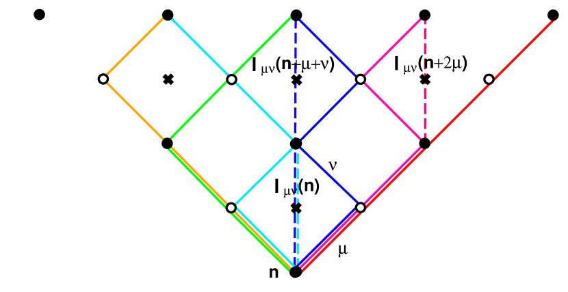
Since the separation between any two adjacent events of the null lattice is light-like, the proper time of a path like $\mathfrak{P}_{L}$ vanishes. To allow for paths that are time-like, additional events of the manifold must be considered. It is natural to include events that bisect the spatial diagonals of plaquettes. In  Fig. 4 these are marked by a cross ($\times$). These additional (centered) events of a plaquette based at the active node $\mathbf{n}$ will be denoted by $\widehat{\mathbf{n}}$. Note that the plaquette is uniquely determined by the events on the path before and after $\widehat{\mathbf{n}}$. The temporal and spatial separation of these center-events to other events of the same plaquette are readily computed in terms of the null lat-frames of a single inertial system.

Consider a $\mu\nu$-plaquette based at the active node $\mathbf{n}$ with ”center” $\widehat{\mathbf{n}}$. Viewed from an inertial system with origin at the active node $\mathbf{n}$, the event proper time to the event $\hat{\mathbf{n}}$ is $\Delta s=\sqrt{-{\textstyle\frac{1}{2}}E_{\mu}(\mathbf{n})\cdot E_{\nu}(\mathbf{n})}={\textstyle\frac{1}{2}}\ell_{\mu\nu}(\mathbf{n})>0$. Due to  Eq.(46) the proper time between $\widehat{\mathbf{n}}$ and $\mathbf{n}^{\prime}=\mathbf{n}+\mu+\nu$ on the same plaquette. determined in the inertial system at $\mathbf{n}^{\prime}$, is the same $\Delta s^{\prime}=\sqrt{-{\textstyle\frac{1}{2}}\widetilde{E}_{\mu}(\mathbf{n})\cdot\widetilde{E}_{\nu}(\mathbf{n})}={\textstyle\frac{1}{2}}\ell_{\mu\nu}(\mathbf{n})=\Delta s$ . Note that the proper time $2\Delta s=\ell_{\mu\nu}$ between $\mathbf{n}$ and $\mathbf{n}^{\prime}$ is largest for a path that passes through the central node $\widehat{\mathbf{n}}$ of the diagonal. The spatial separation of the event at $\widehat{\mathbf{n}}$ from the events labeled by $\mathbf{n}+\mu$ and $\mathbf{n}+\nu$ also181818Although the $SL(2,\mathbb{C})\,$invariant square of the distances have opposite sign, proper times and spatial lengths here are both defined positive. is ${\textstyle\frac{1}{2}}\ell_{\mu\nu}(\mathbf{n})$.

Extending  Eq.(84) to include paths $\mathfrak{\bar{P}}_{L}$ of depth $L$ between two (active) nodes $\mathbf{n}$ and $\mathbf{n}^{\prime}$ that can pass through central nodes, we consider contiguous lists of events of the form,

$$\mathfrak{\bar{P}}_{L}=\{\mathbf{n}_{0},\dots,\mathbf{n}_{j-1},\widehat{\mathbf{n}}_{j},\mathbf{n}_{j+1},\dots,\mathbf{n}_{k-1},\widehat{\mathbf{n}}_{k},\mathbf{n}_{k+1},\dots,\mathbf{n}_{L}\}\ .$$ (85)

Note that any center-event $\widehat{\mathbf{n}}_{k}$ in this list is flanked by two (active) nodes of the same plaquette. We can select the causal paths from an (active) node $\mathbf{n}_{0}$ to an active node $\mathbf{n}_{L}\geq\mathbf{n}_{0}$ by demanding that each of its increments either be light- or time-like in the forward direction. A causal path $\mathfrak{C}_{L}$ thus is a list of $L$ contiguous events of the form191919Every causal path between two active nodes $\mathbf{n}$ and $\mathbf{n}^{\prime}\geq\mathbf{n}$ has the same depth $L=\sum_{\mu}h_{\mu}$ .,

$$\mathfrak{C}_{L}=\{\mathbf{n}_{0},\dots,\mathbf{n}_{j-1},\widehat{\mathbf{n}}_{j},\mathbf{n}_{j+1},\dots,\mathbf{n}_{k-1},\widehat{\mathbf{n}}_{k},\mathbf{n}_{k+1},\dots,\mathbf{n}_{L}\}\ ,$$ (86)

with time- or light-like positive increments only. Every point of a causal path thus is in the immediate future of the previous one. The adjacent active events determine the plaquette ($\mu\nu$) on which a center-event $\widehat{\mathbf{n}}_{k}$ is located. The proper time $s(\mathfrak{C}_{L})$ of a causal path is the sum of the proper times of its increments,

$$s(\mathfrak{C}_{L}):=\sum_{\widehat{\mathbf{n}}_{k}\in\mathfrak{C}_{L}}2\sqrt{-{\textstyle\frac{1}{2}}E_{\mu}(\mathbf{n}_{k-1})\cdot E_{\nu}(\mathbf{n}_{k-1})}=\sum_{\widehat{\mathbf{n}}_{k}\in\mathfrak{C}_{L}}|f_{\mu\nu}(\mathbf{n}_{k-1})|\geq 0\ ,\ \ \text{with }\mathbf{n}_{k+1}=\mathbf{n}_{k-1}+\mathbf{\Delta}_{\mu}+\mathbf{\Delta}_{\nu}\ .$$ (87)

The sum is over center-nodes of the path only, since all other increments are null and do not contribute to the proper time. Note that the proper time defined by  Eq.(87) is an observable composed of basic invariants of the lattice. The consistency condition of  Eq.(46) has to be satisfied, but the backward lat-frames of the configuration need not be reconstructed to define this proper time. That  Eq.(87) is a physically sensible definition of the proper time of a causal path can be seen by choosing inertial systems (a gauge), in which the spatially separate events of any traversed plaquette are simultaneous (we proved in  Sect.VI that this path-dependent choice of gauge is possible and unique up to spatial rotations). In the corresponding inertial systems, the proper time between the two active nodes also gives the spatial extent $\ell_{\mu\nu}(\mathbf{n})$ of the plaquette.  Eq.(87) merely defines the proper time of the whole path as the sum of these increments202020Note in this context that for a $34$-plaquette in an inertial system at $\mathbf{n}$ that satisfies  Eq.(78), $|f_{34}(\mathbf{n})|=|\xi_{3}^{1}|^{2}+|\xi_{3}^{2}|^{2}=\tau_{3}=\tau_{4}$. .  Fig. 8 depicts some causal paths of depth $L=4$ and their proper times.

Refer to caption
Figure 8: (Color online) Nodes of the duoverse related to $\mathbf{n}$ by causal paths in the $\mu\nu$-plane. Several causal paths of depth $L=4$ through active nodes ($\bullet$), passive nodes ($\circ$) and central nodes ($\times$) are shown in different colors. Solid sections of a path do not contribute to its proper time. Dashed sections of a path through a central node contribute $\ell_{\mu\nu}$ to the proper time, where $\ell_{\mu\nu}>0$ is the spatial separation between the two passive nodes of the same plaquette. In the universe all nodes are active and there is a central node on each plaquette.

For any particular consistent causal lattice configuration one may select the lattice path with the longest proper time and define the geodesic distance between two causally related nodes as,

$$d(\mathbf{n},\mathbf{n}^{\prime}):=\max_{\mathfrak{\bar{C}}_{L}:\mathbf{n}\rightarrow\mathbf{n}^{\prime}}s(\mathfrak{\bar{C}}_{L})\ ,$$ (88)

where $L=\sum_{\mu}h_{\mu}$ is the depth of all causal paths that relate $\mathbf{n}$ to $\mathbf{n}^{\prime}$. The number of causal paths that connect a given pair of (active) nodes is finite but can be rather large: the number of causal paths with vanishing proper time already is $L!/(h_{1}!h_{2}!h_{3}!h_{4}!)$. In general $d(\mathbf{n},\mathbf{n}^{\prime})=0$ only if $\mathbf{n}^{\prime}=\mathbf{n}+L\mathbf{\Delta}_{\mu}$, but the geodesic distance between some events may be quite small (of Planck size) even for a large number of steps $L$. From a macroscopic point of view such events essentially are on light-like geodesics.

These considerations apply to a given causal configuration only. Since the weight $e^{iS_{\rm HP}}$ of the Lorentzian lattice is complex, the weighted proper time of a given path between two causally related nodes in general could be complex even though it is a positive real quantity for any particular configuration. Stationary phase approximation suggests that the average proper time is (almost) real for sufficiently deep paths, but could be complex for paths of a few steps. The geodesic distance between close-by nodes depends on the configuration and a physical interpretation of correlation functions between two local observables (say $V(\mathbf{n})$ and $V(\mathbf{n}^{\prime})$) such as

$$\langle V(\mathbf{n})V(\mathbf{n}^{\prime})\rangle\ ,$$ (89)

is hardly possible if the geodesic distance between the lattice points $\mathbf{n}$ and $\mathbf{n}^{\prime}$ fluctuates. One perhaps instead should consider conditional amplitudes like,

$$\langle V(\mathbf{n})V(\mathbf{n}^{\prime})\rangle_{d(\mathbf{n},\mathbf{n}^{\prime})=\tau}\ .$$ (90)

Here the correlator is the (complex) weighted average with respect to configurations whose geodesic distance between the two lattice vertices $\mathbf{n}$ and $\mathbf{n}^{\prime}$ is given by $\tau$. One then could ask how this amplitude depends on $\tau>0$. The conditional amplitude of  Eq.(90) thus gives the correlation between the local 4-volumes of a subset of all causal configurations. Since the theory is not invariant under translations, the conditioning of amplitudes in general will have to be more severe. It may in particular be necessary to fix the geodesic distance of an event to the Big Bang, because correlators like that in  Eq.(90) almost surely depend on the epoch.

For nodes $\mathbf{n}$ and $\mathbf{n}^{\prime}$ related by causal paths of great depth $L$, the conditioning in  Eq.(90) may not be that important, because the geodesic distance in this case is relatively well defined and should not differ much from the leading semi-classical estimate. Conditional and unconditional correlators coincide in this approximation. One thus perhaps can compute the asymptotic large-distance behavior of amplitudes in the conventional fashion. However, only conditioned correlators may be well defined at short distances on a finite lattice.

VIII Integration Measure, Regularization and Orientation

To compute expectation values of $SL(2,\mathbb{C})\,$-invariant observables, an integration measure for the spinors and transport matrices must be specified. Contrary to ordinary lattice gauge theories with fixed lattice spacing, the short-distance behavior of the present lattice model in addition needs to be regularized in a coordinate invariant geometrical fashion. The proper measure satisfies both objectives and in addition ensures that configurations of this lattice model correspond to oriented triangulated manifolds.

VIII.1 Polar Parametrization of Spinors

In a ”spherical” parametrization of the spinors by their magnitude $\tau$ and (real) angles $0\leq\psi_{\mu}<2\pi$, $0\leq\varphi_{\mu}<2\pi$, $0\leq\theta_{\mu}\leq\pi$,

$$\xi_{\mu}(\mathbf{n})=\sqrt{\tau_{\mu}(\mathbf{n})}e^{i\psi_{\mu}(\mathbf{n})}\widehat{\xi}_{\mu}(\mathbf{n})=\sqrt{\tau_{\mu}(\mathbf{n})}e^{i\psi_{\mu}(\mathbf{n})}\left(\begin{smallmatrix}e^{-i\varphi_{\mu}(\mathbf{n})/2}\cos(\theta_{\mu}(\mathbf{n})/2)\\ e^{i\varphi_{\mu}(\mathbf{n})/2}\ \ \sin(\theta_{\mu}(\mathbf{n})/2)\end{smallmatrix}\right),$$ (91)

$\tau_{\mu}(\mathbf{n})$ is the only non-compact variable,

$$0<\tau_{\mu}(\mathbf{n})=\sum_{A=1}^{2}|\xi_{\mu}^{A}(\mathbf{n})|^{2}=-i{\rm Tr}E_{\mu}(\mathbf{n})\ .$$ (92)

$U^{4}(1)$-invariance of physical observables implies that they do not depend on the phase $\psi_{\mu}(\mathbf{n})$ of the spinors. In spherical coordinates the singular anti-hermitian matrix $E_{\mu}(\mathbf{n})$ thus is parameterized by its temporal extent, $\tau_{\mu}$, and the three-dimensional unit vector,

$$\widehat{r}_{\mu}(\mathbf{n})=(\sin\theta_{\mu}(\mathbf{n})\cos\varphi_{\mu}(\mathbf{n}),\sin\theta_{\mu}(\mathbf{n})\sin\varphi_{\mu}(\mathbf{n}),\cos\theta_{\mu}(\mathbf{n}))\ ,$$ (93)

which specifies the direction of the null-ray in a local inertial system at $\mathbf{n}$.

In the parametrization of  Eq.(91), the forward null lat-frames may be written,

$$E_{\mu}(\mathbf{n})=i\xi_{\mu}(\mathbf{n})\otimes\xi^{\dagger}_{\mu}(\mathbf{n})=i\tau_{\mu}(\mathbf{n})P_{\mu}(\mathbf{n})\ ,$$ (94)

where the projector $P_{\mu}(\mathbf{n})$ is the matrix,

$$P_{\mu}(\mathbf{n})=P(\widehat{r}_{\mu}(\mathbf{n})):=\frac{1}{2}({\mathbb{1}}-i\vec{\sigma}\widehat{r}_{\mu}(\mathbf{n}))=\frac{1}{2}\left(\begin{smallmatrix}1+\cos(\theta_{\mu}(\mathbf{n}))&e^{-i\varphi_{\mu}(\mathbf{n})}\sin(\theta_{\mu}(\mathbf{n}))\\ e^{i\varphi_{\mu}(\mathbf{n})}\sin(\theta_{\mu}(\mathbf{n}))&1-\cos(\theta_{\mu}(\mathbf{n}))\\ \end{smallmatrix}\right)\ .$$ (95)

Using Eqs. (94) and (95) in  Eq.(39), the 4-volume element $V(\mathbf{n})$ of the 5-simplex formed by the four null vectors of a node is given by,

$$V(\mathbf{n})=\frac{1}{16}\tau_{1}\tau_{2}\tau_{3}\tau_{4}\det\left(\begin{smallmatrix}\widehat{r}_{1}&1\\ \widehat{r}_{2}&1\\ \widehat{r}_{3}&1\\ \widehat{r}_{4}&1\\ \end{smallmatrix}\right)_{\mathbf{n}}=\tau_{1}(\mathbf{n})\tau_{2}(\mathbf{n})\tau_{3}(\mathbf{n})\tau_{4}(\mathbf{n})\widehat{V}(\mathbf{n})\ ,$$ (96)

with

$$\widehat{V}(\mathbf{n})=\frac{1}{16}\det\left(\begin{smallmatrix}\widehat{r}_{1}-\widehat{r}_{4}\\ \widehat{r}_{2}-\widehat{r}_{4}\\ \widehat{r}_{3}-\widehat{r}_{4}\\ \end{smallmatrix}\right)_{\mathbf{n}}=-\frac{i}{48}\sum_{\mu\nu\rho\sigma}\varepsilon(\mu\nu\rho\sigma){\rm Tr}P_{\mu}(\mathbf{n})\varepsilon P_{\nu}(\mathbf{n})\varepsilon P_{\rho}(\mathbf{n})\varepsilon P_{\sigma}(\mathbf{n})\varepsilon\ .$$ (97)

The 4-volume thus is proportional to the three-dimensional volume of a tetrahedron with vertices at the unit vectors $\widehat{r}_{1},\widehat{r}_{2},\widehat{r}_{3}$ and $\widehat{r}_{4}$. It vanishes only when these four points are coplanar and changes sign when a vertex is reflected through the plane of the other three.

In a system where  Eq.(78) holds, the dependence on $\tau_{4}$ and $\widehat{r}_{4}$ can be eliminated. The 4-volume in this case assumes the form,

$$V_{\text{GF}}(\mathbf{n})=\frac{1}{16}\tau_{1}\tau_{2}\tau^{2}_{3}\det\left(\begin{smallmatrix}\widehat{r}_{1}&1\\ \widehat{r}_{2}&1\\ \widehat{r}_{3}&1\\ -\widehat{r}_{3}&1\\ \end{smallmatrix}\right)_{\mathbf{n}}=\frac{1}{8}\tau_{1}(\mathbf{n})\tau_{2}(\mathbf{n})\tau^{2}_{3}(\mathbf{n})\ \left(\widehat{r}_{1}(\mathbf{n})\times\widehat{r}_{2}(\mathbf{n})\right)\cdot\widehat{r}_{3}(\mathbf{n})\ ,$$ (98)

and is proportional to the three-volume spanned by the spatial components of $E_{1}(\mathbf{n}),\;E_{2}(\mathbf{n})$ and $E_{3}(\mathbf{n})$.

VIII.2 Localized Lattice Integration Measure

Since transport matrices and lat-frames are invariants, the diffeomorphism group does not constrain the integration measure. However, invariance under the $SL(2,\mathbb{C})\,$structure group and the local $U^{4}(1)$ to a large extent dictates the local integration measure of this lattice model. The invariant integration measure for the $SL(2,\mathbb{C})\,$transport matrices is the Haar measure of $SL(2,\mathbb{C})\,$. For matrices in the fundamental representation of $SL(2,\mathbb{C})\,$of the form,

$$U=\left(\begin{smallmatrix}\alpha&\beta\\ \gamma&\delta\end{smallmatrix}\right),\ \text{ with }(\alpha,\beta,\gamma,\delta)\in\mathbb{C}^{4}\ \text{ and }\alpha\delta-\beta\gamma=1\ ,$$ (99)

the left and right invariant Haar measure is proportional toBarut and Raczka ,

$$d\mu[U]=\delta^{2}(1+\beta\gamma-\alpha\delta)d\alpha d\alpha^{*}d\beta d\beta^{*}d\gamma d\gamma^{*}d\delta d\delta^{*}=d\alpha d\alpha^{*}d\beta d\beta^{*}d\gamma d\gamma^{*}/|\alpha|^{2}\ .$$ (100)

For the purpose of analytic continuation of $SL(2,\mathbb{C})\,$to a compact $SU(2)_{L}\times SU(2)_{R}$ it may be more convenient to parameterize $U\in\textrm{$SL(2,\mathbb{C})\,$}$ in terms of 5 compact Euler angles $0\leq\psi<2\pi,0\leq\theta,\bar{\theta}<\pi,0\leq\phi,\bar{\phi}<4\pi$ and a single non-compact variable $0\leq\bar{\psi}<\infty$,

$$U=e^{\sigma_{3}\psi/2}\;e^{\sigma_{2}\theta/2}\;e^{\sigma_{3}\phi/2}\;e^{i\sigma_{3}\bar{\psi}/2}\;e^{\sigma_{2}\bar{\theta}/2}\;e^{\sigma_{3}\bar{\phi}/2}\ ;\ \ U^{\dagger}=e^{-\sigma_{3}\bar{\phi}/2}\;e^{-\sigma_{2}\bar{\theta}/2}\;e^{i\sigma_{3}\bar{\psi}/2}e^{-\sigma_{3}\phi/2}\;e^{-\sigma_{2}\theta/2}\;e^{-\sigma_{3}\psi/2}\ \ .$$ (101)

The corresponding $SL(2,\mathbb{C})\,$-invariant Haar measure is proportional to,

$$d\mu[U]=d\psi\sin\theta d\theta d\phi d\bar{\psi}\sin\bar{\theta}d\bar{\theta}d\bar{\phi}\ ,$$ (102)

over the entire parameter domain.212121Formally the analytic continuation of $SL(2,\mathbb{C})\,$to compact $SU(2)_{L}\times SU(2)_{R}$ corresponds to a change of the integration contour for $\bar{\psi}$ from the positive real axis to the imaginary one, $\bar{\psi}\rightarrow\pm i\bar{\psi}$. However, this ”Wick rotation” of the high-dimensional integral must be carried out with careWitten (2011) for the contribution from the contour at infinity to vanish. Although important for numerical simulations, this article does not further pursue the analytic continuation of the lattice integrals.

Invariance under $SL(2,\mathbb{C})\,$transformations of  Eq.(17) furthermore greatly restricts the local integration measure for the null-vectors $E_{\nu}(\mathbf{n})$ and for the corresponding spinors. For the spherical representation of  Eq.(94) the $SL(2,\mathbb{C})\,$-invariant measure at each lattice site is proportional to,

$$d\mu[E_{\nu}]\propto d^{4}E_{\nu}\ \delta^{+}(E_{\nu}\cdot E_{\nu})\propto\tau_{\nu}d^{+}\tau_{\nu}\;d\Omega(\widehat{r}_{\nu})\ .$$ (103)

$d\Omega(\widehat{r}_{\nu})=\sin(\theta_{\nu})d\theta_{\nu}d\varphi_{\nu}$ here is the $SO(3)$-invariant measure on $S_{2}$ in spherical coordinates and $d^{+}\tau_{\mu}=\Theta[\tau_{\mu}]d\tau_{\mu}$. The corresponding $SL(2,\mathbb{C})\,$-invariant measure for the spinors includes the integration measure for the phase $\psi_{\nu}$. Local $U(1)$ invariance requires that,

$$d\mu[\xi_{\nu}]\propto\tau_{\nu}d^{+}\tau_{\nu}d\psi_{\nu}d\Omega(\widehat{r}_{\nu})\ ,$$ (104)

where the domain of the three angles is $0\leq\psi_{\nu}\leq 2\pi,0\leq\theta_{\nu}\leq\pi$ and $0\leq\varphi_{\nu}<2\pi$. In the gauge of  Eq.(78), the local integration measure for the spinors at each node thus is of the form,

$$\int_{0}^{\infty}\tau_{3}^{3}d\tau_{3}\int_{0}^{\infty}\tau_{2}d\tau_{2}\int_{0}^{\infty}\tau_{1}d\tau_{1}\int_{S_{2}}d\Omega_{3}\int_{S_{2}}d\Omega_{2}\int_{S_{2}}d\Omega_{1}\int_{0}^{2\pi}d\psi_{3}\int_{0}^{2\pi}d\psi_{1}\;\rho(V)\ .$$ (105)

The local $U^{4}(1)$-invariance of observables was here exploited to set $\psi_{2}=-\psi_{1}$ and $\psi_{4}=-\psi_{3}$ and the determinant of the Hessian of  Eq.(77) leads to the weight proportional to $\tau_{3}^{3}$ in  Eq.(105). The measure of  Eq.(105) distinguishes $\mu=3$ from $\mu=1,2$, since the partial $SL(2,\mathbb{C})\,$gauge-fixing of  Eq.(78) does not treat the lat-frames equitably.

Requiring $SL(2,\mathbb{C})\,$- invariance thus determines the local integration measure up to an invariant density. $\rho(V)\geq 0$ in  Eq.(105) is a positive semi-definite function of local $SL(2,\mathbb{C})\,$-invariants. All these local invariants are constructed from $f_{\mu\nu}(\mathbf{n})$ and they include the 4-volume $V(\mathbf{n})$ of  Eq.(96). Note that $\rho(V)$ in the presnt model generally will depend on the local 4-volume: in the first order formulation of Appendix B, auxiliary 0-forms are introduced to linearize matter actions. Integrating over such non-dynamical fields leads to a factor of $1/\sqrt{V(\mathbf{n})}$ in the lattice measure at each site for each auxiliary degree of freedom. $\rho(V)$ must compensate for the introduction of such non-dynamical and unphysical degrees of freedom. Note that the dependence of the classical lattice action on the cosmological constant could also be absorbed in $\rho(V)$.

Assuming that $\rho(V<0)=0$ resolves the sign ambiguity of the volume element and ensures that all lattice configurations correspond to oriented complexes. The next section exploits the fact that the critical limit of the model depends on the asymptotic behavior of $\rho(V)$ for $V\rightarrow 0$ only.

The partially localized integration measure of  Eq.(105) is manifestly invariant under the residual $SU(2)$ structure group. The local rotational invariance of observables therefore can be exploited to completely localize the residual $SU(2)$ structure group. This localization of a compact group is not compatible Schaden (1999); Neuberger (1987) with a BRST-construction, but one evidently can choose lat-frames in which the $\mu=3$ ray has spherical coordinate $\theta_{3}=0$, with $\varphi_{3}$ undetermined, and the $\mu=2$ ray defines the $xz$-plane with $\varphi_{2}=0$. Renaming $\varphi_{1}\rightarrow\varphi$, the local 4-volume of  Eq.(98) in this complete gauge is given by,

$$V^{\prime}_{\text{GF}}(\mathbf{n})=\frac{1}{8}\tau_{1}(\mathbf{n})\tau_{2}(\mathbf{n})\tau^{2}_{3}(\mathbf{n})\sin{\theta_{1}(\mathbf{n})}\sin{\theta_{2}(\mathbf{n})\sin{\varphi(\mathbf{n})}}\ .$$ (106)

The local volume element $V$ in this case is positive for $0<\varphi<\pi$ and negative for $\pi<\varphi<2\pi$ (since $0\leq\theta_{1},\theta_{2}<\pi$). One thus can restrict to oriented lattice configurations by the integration domain of $\varphi$ ! For oriented configurations, the integrals of the remaining spinor variables at each active node $\mathbf{n}$ of the fully localized model are,

$$\int_{0}^{\infty}\tau_{3}^{3}d\tau_{3}\int_{0}^{\pi}d\varphi\int_{0}^{\infty}\tau_{2}d\tau_{2}\int_{0}^{\infty}\tau_{1}d\tau_{1}\int_{0}^{\pi}\sin{\theta_{2}}d\theta_{2}\int_{0}^{\pi}\sin{\theta_{1}}d\theta_{1}\int_{0}^{2\pi}d\psi_{3}\int_{0}^{2\pi}d\psi_{1}\;\rho(V^{\prime}_{\text{GF}})\ ,$$ (107)

where the spinors associated with a node are parameterized as,

$$\xi_{4}=\sqrt{\tau_{3}}e^{-i\psi_{3}}\left(\begin{smallmatrix}0\\ 1\end{smallmatrix}\right)\ ;\ \xi_{3}=\sqrt{\tau_{3}}e^{i\psi_{3}}\left(\begin{smallmatrix}1\\ 0\end{smallmatrix}\right)\ ;\ \xi_{2}=\sqrt{\tau_{2}}e^{-i\psi_{1}}\left(\begin{smallmatrix}\cos{(\theta_{2}/2)}\\ \sin{(\theta_{2}/2)}\end{smallmatrix}\right)\ ;\ \xi_{1}=\sqrt{\tau_{1}}e^{i\psi_{1}}\left(\begin{smallmatrix}e^{-i\varphi/2}\cos(\theta_{1}/2)\\ e^{i\varphi/2}\ \ \sin(\theta_{1}/2)\end{smallmatrix}\right)\ .$$ (108)

Ignoring222222The integrals over $\psi_{1}$ and $\psi_{3}$ in  Eq.(107) are absorbed by the TLT of Eq.(67) that enforces the consistency condition. Observables do not depend on these angles. the remaining spinor angles $\psi_{1}$ and $\psi_{3}$,  Eq.(107) is an integral over the correct number (6 per site) of $SL(2,\mathbb{C})\,$-invariant degrees of freedom.

VIII.3 Invariant Regularization

Although discrete, this lattice model is not necessarily regular at short distances and may not possess a critical limit. Configurations for which the local lattice volume $V(\mathbf{n})$ is arbitrary small are not suppressed by triangulating the manifold and may dominate the lattice integral. A minimal coarseness must be imposed to avoid the associated UV-instability and obtain a UV-finite lattice model. The UV stability of the model thus is related to the behavior of the density $\rho(V)$ at small $V$. Note that the local 4-volume element $V(\mathbf{n})$ is invariant under reparametrization because the lat-frames are (see  Eq.(15)).

Since events are defined by the intersection of light-cones, one cannot demand that the local 4-volume be of fixed size. A viable model requires only that $\rho(V)$ suppress configurations with small local 4-volumes $V(\mathbf{n})$. In the critical limit when the number of lattice sites $N$ becomes large, while the total 4-volume of the universe remains constant, only the asymptotic behavior of $\rho(V)$ for small $V$ matters. I will assume that it is power-like

$$\rho(V\sim 0)\propto\Theta[V]\,V^{\gamma}(1+{\cal O}(V))\ ,$$ (109)

with an a priori unknown global exponent $\gamma$ that could depend on the number of lattice sites $N$ and on the cosmological constant $\lambda$ (and possibly other lattice couplings).

In the complete gauge of  Eq.(78), the asymptotic UV behavior of the density in  Eq.(109) leads to lattice integrals at each (active) node of the form,

$$\int_{0}^{\infty}\tau_{3}^{3+2\gamma}d\tau_{3}\int_{0}^{\pi}(\sin{\varphi})^{\gamma}d\varphi\int_{0}^{\infty}\tau^{1+\gamma}_{2}d\tau_{2}\int_{0}^{\infty}\tau^{1+\gamma}_{1}d\tau_{1}\int_{0}^{\pi}(\sin{\theta_{2}})^{1+\gamma}d\theta_{2}\int_{0}^{\pi}(\sin{\theta_{1}})^{1+\gamma}d\theta_{1}\int_{0}^{2\pi}d\psi_{3}\int_{0}^{2\pi}d\psi_{1}\ ,$$ (110)

where the parametrization of the spinors is given in  Eq.(108).

For a lattice with $N$ sites, the total 4-volume of the uni- (or duo-)verse will be constant on a curve $\gamma(\lambda;N)$. The intersection of these curves in the limit $N\rightarrow\infty$ then formally yields the critical points $\gamma_{*},\lambda_{*}$ of the continuum theory (if a critical limit exists).

IX The Strong Coupling Limit $\lambda\rightarrow\infty$

It is interesting to consider the (naïve) strong coupling limit of this model in which curvature terms of the action are simply neglected. The lattice action in this limit is ultra-local and the model has a number of symmetries232323Although the evolution of our universe is believed to be dominated by the cosmological term long after the Big Bang, we here consider rather small lattices that hardly provide a faithful representation of the universe in its later stages.. These enable us to define a finite lattice model and establish that $\gamma^{*}=-2$ in this strong coupling limit. At this critical value of the exponent $\gamma$ the 4-volume of the universe collapses for any lattice with a finite number of sites.

Using  Eq.(108) and the definition of  Eq.(32a), the lattice integrals of  Eq.(110) at each active node $\mathbf{n}$ may be written in terms of the invariant lengths $\ell^{2}_{\mu\nu}(\mathbf{n})$ of  Eq.(33) as,

$$\left(\prod_{\mu<\nu}\int_{0}^{\infty}d\ell^{2}_{\mu\nu}\right)V^{\gamma-1}\Upsilon(a,b,c)\ ,$$ (111)

with $\Upsilon$ defined in  Eq.(73) and,

$$a(\mathbf{n})=\ell_{12}(\mathbf{n})\ell_{34}(\mathbf{n}),\ \ \ b(\mathbf{n})=\ell_{13}(\mathbf{n})\ell_{24}(\mathbf{n}),\ \ \ c(\mathbf{n})=\ell_{14}(\mathbf{n})\ell_{23}(\mathbf{n})\ .$$ (112)

Expressed by the lengths, the local invariant volume element of  Eq.(39) is,

$$V(\mathbf{n})=\sqrt{-\det(\ell^{2}_{\mu\nu}(\mathbf{n}))}=\left(2a^{2}b^{2}+2b^{2}c^{2}+2c^{2}a^{2}-a^{4}-b^{4}-c^{4}\right)_{\mathbf{n}}^{1/2}\ .$$ (113)

Note that the triangle inequalities imposed by the $\Upsilon$-distribution in  Eq.(111) arise automatically in the change of integration variables. They ensure that the volume in  Eq.(113) is real. The fact that the localized measure of  Eq.(110) can be expressed in terms of $SL(2,\mathbb{C})\,$-invariants indirectly confirms that the localization was unique.

Since the cosmological part of the lattice action $S_{SC}\sim\sum_{\mathbf{n}}V(\mathbf{n})$ is ultra local, the generating function of the naïve strong coupling limit decomposes into a product of independent generating functions for each site when consistency constraints are ignored. We restrict the configuration space to consistent complexes (that represent triangulated causal manifolds) by imposing the inequalities of  Eq.(V.1), respectively  Eq.(50). The generating function $Z_{SC}[\lambda;\gamma]$ in the naïve strong coupling limit we are considering formally thus is,

$$Z_{SC}[\lambda;\gamma]=\prod_{\mathbf{n}\in\bar{\mathbf{\Lambda}}}\left[\left(\prod_{\mu<\nu}\int_{0}^{\infty}d\ell^{2}_{\mu\nu}\right)V^{\gamma-1}e^{-4i\lambda V}\Upsilon(a,b,c)\Upsilon(\widetilde{a},\widetilde{b},\widetilde{c})\right]_{\mathbf{n}}\ ,$$ (114)

where $\widetilde{a},\widetilde{b}$ and $\widetilde{c}$ are given by the $\widetilde{\ell}_{\mu\nu}(\mathbf{n})=\ell_{\mu\nu}(\mathbf{n}-\mu-\nu)$ as in  Eq.(V.2). The $\Upsilon$-distributions of  Eq.(73) ensure that the integral in Eq.(114) is over configurations $\{\ell_{\mu\nu}(\mathbf{n})\}$ that correspond to triangulated causal manifolds only. Note that the triangle inequalities of  Eq.(73) actually depend on the squares of the lengths $\ell^{2}_{\mu\nu}$ only, as might be expected since the continuum action in this limit depends on the metric $g_{ik}$ only.

For a hypercubic lattice with $N^{4}$ active sites and periodic boundary conditions, the variables of  Eq.(112) and  Eq.(V.2) are invariant under $3N^{3}$ continuous scaling symmetries. These form an Abelian dilation group generated by,

$\displaystyle\delta^{(i)}_{\mathbf{n}}\ell_{i4}(\mathbf{n}^{\prime})=\ell_{i4}(\mathbf{n}^{\prime})\ \ \ \delta^{(i)}_{\mathbf{n}}\ell_{jk}(\mathbf{n}^{\prime})=-\ell_{jk}(\mathbf{n}^{\prime}),$ $\displaystyle\text{for all }\mathbf{n}^{\prime}=\mathbf{n}+q\Delta^{(i)}\ \text{with }q\in\mathbb{Z}\ \text{and }\{i,j,k\}=\{1,2,3\}$
$\displaystyle\text{where }\Delta^{(i)}:=\mathbf{\Delta}_{j}+\mathbf{\Delta}_{k}-\mathbf{\Delta}_{i}-\mathbf{\Delta}_{4}\ .$ (115)

This definition of the generators may appear to single out the $4$-th lattice direction, but in fact implies only that $\ell_{\mu\nu}$ scales oppositely to $\ell_{\rho\sigma}$, with $\{\mu,\nu,\rho,\sigma\}=\{1,2,3,4\}$. By definition $\delta_{\mathbf{n}}^{(i)}\equiv\delta_{\mathbf{n}^{\prime}}^{(i)}$ if $\mathbf{n}$ and $\mathbf{n}^{\prime}$ differ by a multiple of $\Delta^{(i)}$. There thus are only $3N^{3}$ independent generators on a periodic $N^{4}$ lattice and the number of these scaling symmetries is proportional to the number of sites on the 3-dimensional surface of a hyper-cubic lattice. If one ignores the consistency constraints, the number of independent scaling generators increases to $3N^{4}$ and is proportional to the number of lattice sites.

One readily verifies that the integration measure $\prod_{\mathbf{n},\mu<\nu}\int_{0}^{\infty}d\ell^{2}_{\mu\nu}$ of  Eq.(114) is invariant under the dilation group generated by  Eq.(IX). The periodic lattice thus is invariant under $3N^{3}$ non-compact scaling symmetries and the generating function of  Eq.(114) diverges.

Refer to caption
Figure 9: Conic lattice: an impressionist rendering of the conic part of the 4-dimensional universe that is causally connected to the Big Bang (the event labeled by (0,0,0,0)). [This figure does not represent results of a numerical simulation.] The four ”spinal” null rays on the light cone emanating from the Big-Bang event are depicted together with events on them. Spatial hyperplanes labeled by their depth $L$ are indicated schematically. Note that these hyperplanes do not correspond to cosmic time because the vertices of the spatial tetrahedrons of a null-simplex generally are not simultaneous in any inertial system. The sketch presumes that these hyperplanes rapidly approach $S_{3}$-hyperspheres with increasing lattice depth. The connected part of the duoverse sketched here is rather small with a maximal depth $L=7$, that is all its events can be reached in $\leq 7$ light-like steps from the Big Bang.

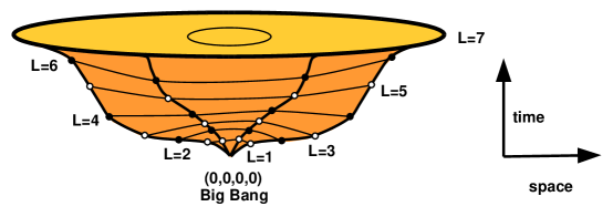
However, the expectation of observables that are invariant under these scaling symmetries, such as any lattice 4-volume, can be computed by localizing the integrals with respect to the scaling group. More interestingly, this dilation group generally is broken by boundary conditions at the ”surface” of the lattice. For physical reasons, we would like to model the causally connected part of the universe by a conic four-dimensional lattice like the one sketched in  Fig. 9. This conic section is obtained by standing a hypercubic lattice on one of its corners and cutting it off at the spatial hyperplane with depth $L_{\text{max}}$; the apex at $\mathbf{n}=(0,0,0,0)$ of the cone in this simple model represents the Big Bang (BB), all other events on the lattice being causally related to it.

The quantities $a,b,c$ of  Eq.(112) are invariant under the scaling symmetries by construction and the 4-volume of  Eq.(113) is as well. $V^{2}(\mathbf{n})$ furthermore is a quadratic form in $a^{2},b^{2},c^{2}$ which in addition is invariant under a local SL(2,R) symmetry. Although this local SL(2,R) may be an accidental symmetry of the action and explicitly broken by curvature contributions, it also is a non-compact symmetry of the local integration measure without consistency constraints. If consistency constraints are imposed, only a subgroup of local SL(2,R) transformations at boundary nodes is preserved.

In Appendix E the scaling symmetries of  Eq.(IX) and the local SL(2,R) are examined in detail. It is found that these non-compact residual symmetries can be localized by imposing boundary conditions on the cone. Viewing these boundary conditions as a localization by the symmetry, one can adjust the integration measure so that the expectation of invariant observables does not depend on them. The boundary conditions of  Eq.(158) effectively identify parts of faces of the global spatial tetrahedron of given depth $L$. Note that this identification turns the triangulated 3-dimensional spatial hyperplane of depth $L$ of the hypercubic lattice we started with into a triangulated closed 3-manifold.

Ignoring restriction of the integration domain imposed by $\Upsilon(\widetilde{a},\widetilde{b},\widetilde{c})$, the generating function $Z_{SC}$ of  Eq.(114) factorizes in generating functions at each site. The local SL(2,R) and scaling symmetries in this case (see Appendix E) allow one to deduce that,

$$Z_{SC}[\lambda;\gamma]=\left(\frac{z(\gamma)}{\lambda}\right)^{N(\gamma+2)}\ ,$$ (116)

where $N$ is the number of sites of the lattice and $z(\gamma)$ for $\gamma>-2$ is a finite integral that does not depend on $\lambda$. From  Eq.(116), the expected 4-volume of the lattice universe at strong coupling thus is given by,

$$\langle iV^{\text{Univ.}}\rangle_{SC}=-\frac{1}{4}\frac{\partial}{\partial\lambda}\ln Z_{SC}[\lambda;\gamma]=\frac{(\gamma+2)N}{4\lambda}\ ,$$ (117)

when consistency constraints are ignored. The variance of the total 4-volume in this case is,

$$\langle(iV^{\text{Univ.}})^{2}\rangle_{SC}-\langle iV^{\text{Univ.}}\rangle^{2}_{SC}=\frac{\partial^{2}}{16\partial\lambda^{2}}\ln Z_{SC}[\lambda;\gamma]=\frac{(\gamma+2)N}{16\lambda^{2}}=\frac{\langle iV^{\text{Univ.}}\rangle_{SC}}{4\lambda}\geq 0\ .$$ (118)

The standard interpretation of $Z_{SC}$ as generating (here depth-) ordered vacuum expectation values Since the expectation of the variance of an hermitian operator ought to be positive,  Eq.(118) implies that the 4-volume of Lorentzian space-time should be associated with an anti-hermitian operator $\hat{V}$ on the Hilbert space and that one measures eigenvalues of $i\hat{V}^{\text{Univ.}}$. This is in keeping with anti-unitary time conjugation in ordinary space-time: although $V(\mathbf{n})$ changes sign, $iV(\mathbf{n})$ is invariant under time reversal. This assignment is compatible with the fact that the generating function of the strong coupling limit turns into a real probability measure upon analytic continuation $4i\lambda\rightarrow\beta>0$.

Figure 10: (Color online) Numerical results for a consistent conic null lattice at strong coupling. The cosmological constant in this numerical study is purely imaginary $\beta=4i\lambda=1$. $\gamma>-2$ is the exponent of the density $\rho(V)\propto V^{\gamma}$. a) Running averages of the invariant subvolumes $\langle V(L)\rangle$ up to depth $L\leq L_{\text{max}}=7$ of the conic lattice. $\langle V(\text{Univ.})\rangle=\langle V(L_{\text{max}})\rangle$ is the average total 4-volume of the conic null lattice. b) Distribution of the total 4-volume of the conic null lattice with $L_{max}=7$ for $\beta=1$ and $\gamma=-1.95$. c) Dependence of the average 4-volume of the null lattice on the depth to the apex of the cone for $\beta=1$ and $\gamma=-1.95$. Note that the 4-volume increases much slower than the number of nodes, $\text{\#nodes}\propto L^{4}$. d) Total 4-volume of the cone up to depth $L_{\text{max}}$ for $\beta=1$ but different exponents $\gamma$. The numerical results for $\gamma=-1.5,-1.8,-1.95$ and a constrained linear fit to them are shown. The extrapolation to vanishing 4-volume at $\gamma=\gamma^{*}\sim-2$ is within the numerical accuracy of the simulations.

Inclusion of the consistency conditions requires numerical simulation even in the naïve strong coupling limit. The numerical results for a conic null-lattice with a maximal depth $L_{\text{max}}=7$ (corresponding to $330$ nodes) for a purely imaginary cosmological constant $\beta=4i\lambda=1$ are presented in  Fig. 10. For these simulations the residual non-compact ”surface” symmetries were all localized in the way described in Appendix E. For Im$\lambda<0$, the corresponding generating function is finite and a Metropolis-Hastings algorithm was used to obtain the shown results for $\beta=1$.  Fig. 10d) shows that the 4-volume of the cone vanishes for $\gamma\sim-2$. The constraints imposed by the consistency conditions therefore do not change the critical exponent $\gamma^{*}$. This is not too surprising, since the consistency constraints are irrelevant for the UV-behavior of the model. To see reasonably fast convergence on the finite lattice, we simulated the model for $\gamma\geq-1.95$.  Fig. 10a) shows expected volumes $\langle V(L)\rangle$ of the cone up to depth $L$, $\langle V(7)\rangle=\langle V^{\text{Univ.}}\rangle$ corresponding to the volume of the null lattice cone itself. These are some of the invariants of this model. They all converge even for $\gamma=-1.95\sim\gamma^{*}$ with the largest fluctuations in $V(0)$, the 4-volume of the simplex whose apex is the Big Bang event. The expected 4-volume of the cone cut at successive slices increases monotonically with depth.  Fig. 10c) shows that does not increase as fast as one might expect if each simplex on average had the same 4-volume (as in the unconstrained case): the number of nodes in each of the sub-volumes is $\text{\#nodes}(L)=1,5,15,35,70,126,210,330$ for $L=0,1,2,3,4,5,6,7$ respectively. Requiring causality thus changes the ”shape” of the Universe even at strong coupling.  Fig. 10b) depicts the (unnormalized) distribution of the total 4-volume $V(7)$ of the lattice cone at $\beta=1$ and $\gamma=-1.95$. It resembles a $\Gamma$-distribution.

Apart from an analytical continuation to real values of $\lambda>0$, the naïve strong coupling limit of this model appears to be accessible numerically. Although devoid of curvature, this limit perhaps is not quite as trivial and uninteresting as might be presumed.

X Summary and Discussion

We considered the triangulation of causal Lorentz manifolds by a null lattice with hypercubic coordination. The nodes of this lattice represent space-time events. Spinors describe the light-like separation to neighboring events in the inertial system of the node at which they are based. Links between nodes are associated with $SL(2,\mathbb{C})\,$transport matrices. The basic $SL(2,\mathbb{C})\,$-invariant observables of this model are those of  Eq.(31). Despite the labeling by a lattice, this is a geometrical construction based on simplexes with four light-like edges and six spatial ones. It is similar to Regge’sRegge (1961); Loll (1998) approach but retains fixed coordination and is based on an internal $SL(2,\mathbb{C})\,$symmetry. As shown in  Sect.II, the triangulation of a causal manifold by light-like signals is physical and coordinate invariant. Macroscopically this method is used to triangulate events by radio signals cemitted from four GPS satellites. Conceptually the only difference here is that the emission events are themselves triangulated in the same fashion instead of being determined by atomic clocks on known orbits.

We investigated two topologically different causal Lorentz manifolds: the universe with a single causally connected component and the duoverse with two. In some ways, the latter is aesthetically more appealing. Its lattice structure topologically is that of a body-centered hypercubic lattice whose two hypercubic sub-lattices are in dual position.The causally disconnected components of the duoverse are described by fields on these mutually dual sub-lattices which are joined by spatial links (on which $SL(2,\mathbb{C})\,$transport matrices live) only. Physical observables in the duoverse are constructed from closed lattice loops and the lattice Hilbert-Palatini action is given by a sum of elementary loops (see  Eq.(43)). The duoverse could offer a novel accommodation for dark matter that does not interact causally with ordinary matter but does affect the observed local curvature. Depending on global boundary conditions, the two causally disconnected components of the duoverse in fact could be conjugate parts of a single non-orientable connected manifold and thus could lead to novel interpretations of the ”arrow of time”, the absence of anti-matter in our part of the duoverse and other globally two-sided phenomena. However, a universe with a single causally connected component seems to be a viable, if less compelling, alternative.

Ignoring global considerations, we first addressed local issues of the lattice theory. In  Sect.V necessary and sufficient conditions for a lattice configuration to represent a triangulated causal manifold were derived. For null lat-frames the local lattice ”metric”, $\ell^{2}_{\mu\nu}=|f_{\mu\nu}(\mathbf{n})|^{2}$, with (complex) amplitudes $f_{\mu\nu}=-f_{\nu\mu}$ defined by  Eq.(32a), is positive semi-definite, vanishing for $\mu=\nu$. The components of this symmetric matrix of spatial lengths satisfy the triangle inequalities of  Eq.(35) with sides given by  Eq.(III). These inequalities are equivalent to demanding that $\det(\ell^{2}_{\mu\nu})\leq 0$, which is necessary for a real local 4-volume. The consistency condition of  Eq.(46) requires that the six spatial lengths on the backward light cone of a node satisfy the corresponding inequalities of  Eq.(V.1), i.e. that the local volume of the corresponding backward null-simplex $\widetilde{ch}(\mathbf{n})$ is real as well. In the spinor formulation, this consistency requirement can be imposed by the TLT of  Eq.(67). The corresponding TLT for null-latframes is obtained in Appendix D. Equivalently, these inequalities may be enforced by Heaviside distributions.

The $SL(2,\mathbb{C})\,$structure group of this lattice theory is not compact and the invariant generating function diverges for any finite number of sites. In  Sect.VI the $SL(2,\mathbb{C})\,$structure group was partially localized to the compact $SU(2)$ subgroup of spatial rotations. This is always possible and a local (equivariant) TFT was constructed that effects this partial gauge fixing. For simplicity and physical reasons, we mainly considered the constraints of  Eq.(78).

The integration measure of this lattice model is strongly constrained by its $SL(2,\mathbb{C})\,$structure group and local $U^{4}(1)$-invariance of the spinors. The measure for the $SL(2,\mathbb{C})\,$transport matrices is the (non-compact) Haar measure. The lattice integration measure for a spherical parametrization of the spinors was derived in  Sect.VIII. The invariant integration measure is determined up to a density $\rho(V)$ that depends on local $SL(2,\mathbb{C})\,$invariants only, and in particular depends on the local 4-volume $V(\mathbf{n})$. We used the gauge condition of  Eq.(78) to localize this $SL(2,\mathbb{C})\,$-invariant integration measure for the spinors. Although not necessary for numerical evaluation, we in addition completely localized the residual compact $SU(2)$-structure group. The spherical parametrization of the spinors in this case is given in  Eq.(108). This completely localized measure for the spinors in fact can be rewritten in terms of the manifestly $SL(2,\mathbb{C})\,$-invariant spatial lengths of  Eq.(33) as in  Eq.(111). The restrictions on the length variables arise automatically in the change of variables.

The apriori undetermined density $\rho(V)$ of the integration measure allows for an invariant regularization of the short-distance behavior of the model that suppresses small local 4-volumes. Assuming the leading dependence of the density $\rho(V)$ for $V\sim 0$ to be power-like as in  Eq.(109), we argue that the lattice integration measure in the spinor parametrization of  Eq.(108) is  Eq.(110). It depends on a parameter $\gamma$. For a lattice with a large number $N$ of sites, the dependence of $\gamma(\lambda,N)$ on the cosmological coupling constant may be determined by demanding that the uni- (or duo-)verse have a given average total observable 4-volume. Critical values $\gamma^{*}$ and $\lambda^{*}$ are points of intersection of these curves as the number of sites $N\rightarrow\infty$.

Sect.IX examined this model in the naïve strong coupling limit, in which the cosmological term dominates and curvature corrections are ignored. The lattice action in this limit is ultra-local and depends on the local 4-volume only.  Eq.(113) gives the local 4-volume in terms of the length variables. Since there is no dependence on transport matrices, the lattice model simplifies in this unphysical limit and the action and measure can be expressed in terms of the six invariant lengths $\ell^{2}_{\mu\nu}(\mathbf{n})$ at each site. We considered a conic lattice where the apex of the topologically hypercubic complex represents the Big Bang and the cone terminates at a spatial depth $L_{\text{max}}$. We systematically found a number of additional non-compact surface symmetries that reflect the fact that there is some freedom in the placement of events on the boundary of the conic manifold: certain choices of events on the boundary can lead to different consistent triangulations of the same manifold and we therefore believe that these lattice symmetries are a consequence of residual diffeomorphisms on the boundary of the manifold. In Appendix E this residual group of lattice symmetries is systematically derived. Since the group of residual symmetries is non-compact, it must be localized before attempting a numerical simulation. We find that this is achieved by imposing certain boundary conditions and adjusting the integration measure so that the expectation of invariant observables does not depend on this localization. In the naïve strong coupling limit these observables include all partial lattice 4-volumes. The boundary conditions on spatial lengths of  Eq.(158) change the topology of the original hyperplane to depth $L$ to that of a closed 3-manifold, much like the identification of the endpoints of a spatial segment to given depth $L$ in the 1+1 dimensional results in a cone with topology $R^{+}\times S_{1}$.

Implementing the additional boundary constraints, numerical simulations on small conic lattices with $L_{\text{max}}\leq 7$ and purely imaginary cosmological constant $4i\lambda=\beta=1$ converge rather well in the naïve strong coupling limit (see  Fig. 10. They indicate that the critical exponent at which the 4-volume of the finite cone vanishes is $\gamma^{*}\simeq-2$ in the consistent model. This is to be expected since the consistency constraints are non-local, and $\gamma^{*}=-2$ when they are relaxed. The numerical results also show that the naïve strong coupling limit of the consistent theory is not trivial: we computed the expected partial 4-volumes of the cone at depths $0\leq L\leq L_{\text{max}}=7$.  Fig. 10c) shows that they increase much slower than the number of simplexes. When consistency conditions are imposed, the generating functional no longer factorizes into independent generating functions for each simplex and the simulations show that the correlations in fact are substantial. These initial numerical results are encouraging and perhaps warrant a more detailed investigation of the model.

A number of issues have to be resolved before this lattice model becomes numerically accessible. Most importantly, the Lorentzian lattice weight of any configuration is a phase $e^{iS_{HP}}$. Lacking an analytic continuation, it is difficult242424New approachesAarts et al. (2010); Greensite (2014); Langfeld et al. (2015); Gattringer and Kniely (2015), originally developed to accommodate a non-vanishing chemical potential in ordinary lattice gauge theories, may help overcome this problem. to numerically evaluate expectations with complex generating functions. The oscillatory integrals in fact may be finite (as are Fresnel integrals) but are difficult to control and evaluate numerically. We so far only verified that the strong coupling limit of this model may be well defined for a purely imaginary cosmological constant.

The complex weight of the Lorentzian model also makes it difficult to define an ”average” proper time between two causally related nodes.  Eq.(87) and  Eq.(88) are a reasonable definition of the proper time of a path and of the geodesic distance between two causally related active nodes of any particular causal configuration only. For an ensemble of such configurations, the proper time of a path between two particular nodes fluctuates and its average could even be a complex quantity. To address the general problem of defining distances in fluctuating geometries, one could consider conditioned amplitudes such as  Eq.(90). In ordinary LGT’s this conditioning has no effect since distances between lattice nodes are known a priori on a space-time manifold that does not fluctuate. However, such a conceptual change in the definition of quantum amplitudes may be crucial in the construction of a quantum field theory based on ensembles of causal manifolds.

Acknowledgements.
I would like to thank D. Zwanziger and P. Cooper for encouragement and a first reading of the manuscript and am deeply indebted to T. Jacobson for constructive criticism. Many improvements and clarifications on the original manuscript derive from our Socratic dialoguecom (2016).

Appendix A Naturalness of the Cosmological Constant in Semi-Classical Quantum Gravity

I argue semi-classically that the incredibly small value of the dimensionless cosmological constant $\lambda=32\pi\ell_{\text{Planck}}^{2}\Lambda\sim 10^{-120}$ is related to the quantum fluctuations of the 4-volume $V_{4}$ of the observable universe. A similar argument is given in Sorkin (2007); Barrow and Shaw (2011), but here I treat the cosmological constant as a coupling constant rather than the expectation of a fluctuating field. This coupling generally will itself depend on the epoch, i.e. on the 4-volume of the observable universe and on the energy density $\rho$ of matter. The infrared free dimensionless coupling $\lambda=32\pi\Lambda\ell^{2}_{P}$ tends to vanish at large cosmic scales but $\lambda$ is assumed to remain large compared to $\ell_{\text{Planck}}^{4}\rho$ (the cosmological term then dominates the evolution of the universe at later stages). Conversely, $\lambda$ could be large but dominated by the energy density in the early universe and lead to a strongly coupled theory that may be difficult to describe (semi-)classically.

Let us therefore just note that fluctuations $\Delta V$ of the 4-volume of the observable universe proportional to the expected 4-volume $\langle V\rangle$,

$$(\Delta V)^{2}:=\langle V^{2}\rangle-\langle V\rangle^{2}=l^{4}_{c}V\ ,$$ (119)

semi-classically imply a cosmological constant

$$\lambda=\Lambda l_{P}^{2}=32\pi\Lambda\ell^{2}_{\text{Planck}}\sim\frac{32\pi(16\pi^{2})\ell_{\text{Planck}}^{4}}{l_{c}^{2}\sqrt{V}}\ .$$ (120)

Eq.(119) follows if the total 4-volume of the universe is composed of a large number, $N$, of volumes $v_{i}$ drawn independently from a single distribution whose variance is finite252525In this case $l^{4}_{c}=(\Delta v)^{2}/\bar{v}$, where $\bar{v}$ is the mean and $(\Delta v)^{2}$ is the variance of this distribution.. That the variance of the 4-volume is proportional to the 4-volume itself continues to hold under somewhat weaker assumptions. Much of the argument in Sorkin (2007) is devoted to deriving  Eq.(119) from causal set theoryBombelli et al. (1987); Carlip (2014). Note that the present model comes close to a concrete realization of this idea: the total number of nearly independent 4-volumes in the strong coupling regime of  Sect.IX is $N=L^{4}$ at depth $L$ where $L$ is proportional to cosmic time at later stages of the evolution.

Averaging over many oscillations of the phase $e^{iS/\hbar}\sim e^{-i\Lambda V_{4}/(8\pi\ell_{\text{Planck}}^{2})}$ in the functional integral would lead to vanishing correlation functions.262626The overall constant phase due to the average 4-volume cancels and is irrelevant in a semi-classical computation of amplitudes. Fluctuations of the cosmological part of the action $S$ thus cannot greatly exceed $h=2\pi\hbar$. Neglecting curvature and matter contributions to the action, the cosmological term provides the main restriction on volume fluctuations.

In epochs dominated by the cosmological part of the action, a semi-classical approach to quantum gravity therefore implies,

$$\frac{\Lambda}{8\pi\ell^{2}_{\text{Planck}}}\Delta V\sim 2\pi\ .$$ (121)

With the estimate  Eq.(119) in  Eq.(121), one then arrives at  Eq.(120).

In  Eq.(120) we introduced the Planck length $\ell_{\text{Planck}}=\sqrt{G\hbar/c^{3}}$. It is the length scale associated with semi-classical gravitational phenomena and it would be unnatural if $l_{c}\ll\ell_{\text{Planck}}$. For the purpose of a rough estimate it suffices to assume that $l_{c}\sim\ell_{\text{Planck}}$, although it may be a few times larger.

It remains to determine the average 4-volume of the observable universe. A somewhat naïve estimate in terms of the radius $r\sim 4.4\times 10^{26}m$ of the observable universe and its age $c\tau\sim 1.3\times 10^{26}m$ yields

$$\lambda\lesssim(32\pi)16\pi^{2}\sqrt{3\ell^{4}_{\text{Planck}}/(4\pi r^{3}c\tau)}\sim 3\times 10^{-120}\ ,$$ (122)

which is about $1/5$ of the value of $\lambda\sim 1.7\times 10^{-119}$ found experimentally272727The coupling $\lambda=\Lambda l_{P}^{2}=32\pi\Lambda\ell^{2}_{\text{Planck}}$ used here is about $32\pi\sim 100$ times the cosmological constant in Planck units. and about twice $(32\pi)/t_{U}^{2}\sim 1.6\times 10^{-120}$ where $t_{U}=8\times 10^{60}$ is the present expansion age of the universe in natural unitsBarrow and Shaw (2011). Considering the crudeness of the estimates, this is encouraging and an indication that gravity is quantized: $\lambda\gg 10^{-120}$ would imply highly suppressed quantum fluctuations and cast doubt on a semi-classical description of quantum gravity. $\lambda\ll 10^{-120}$ on the other hand would imply an unnaturally large universe.

Note that consistent with an infrared free coupling, quantum fluctuations of a 4-volume larger than the observable one ought to be larger and the cosmological constant correspondingly smaller.

The cosmological constant often is considered an effective representation of the vacuum energy density. Its small value compared to typical (often UV-divergent) vacuum energies has been used as an argument for super-symmetric theories. However, the measured effective cosmological constant we are considering does not represent these vacuum energies. As with other coupling constants, only the renormalized cosmological constant can be measured. If quantum gravity is regularized, the measured effective cosmological constant is the difference of a bare cosmological constant and the ground state energy density of matter. It essentially determines the average 4-volume of the observable universe and has little to do with vacuum energies.

Appendix B First order Matter Actions

The first order Hilbert-Palatini action of  Eq.(1) can be written in terms of forms. These diffeomorphism invariant objects retain their geometrical meaning when space-time is discretized. The coupling to matter also can be written in terms of forms and first order matter actions continue to depend polynomially on the co-frame 1-form (with the same sign ambiguity as the Hilbert-Palatini action).

In curved space-time, the first order formulation of the invariant action for a gauge field with curvature two-form ${\cal F}(A)=F_{ik}(A)\;dx^{i}\wedge dx^{k}$ is,

$$S_{A}=\frac{1}{g^{2}}\int_{M}e^{a}\wedge e^{b}\wedge[\frac{1}{6}e^{c}\wedge e^{d}{\rm Tr}{{B}^{ef}}{{B}_{ef}}-2{\rm Tr}{{B}^{cd}}{\cal F}(A)]\varepsilon_{abcd}\ ,$$ (123)

where the trace is over internal degrees of freedom and $B_{ab}=-B_{ba}$ are auxiliary 0-forms. A shift of the auxiliary fields leads to the equivalent and more familiar non-polynomial action,

$$S_{A}=\frac{1}{g^{2}}\int_{M}d^{4}x\;\text{det}(e)\;{\rm Tr}[{{F}_{ik}}(A){{F}^{ik}}(A)-4{{B}^{ab}}{{B}_{ab}}]\ ,\ \text{with}\ \ F^{ik}(A)=g^{il}g^{km}F_{lm}(A)\ ,$$ (124)

if the co-frame is invertible. The first order action of  Eq.(123) thus differs from the more conventional quadratic action by a local correction to the cosmological constant that depends on the auxiliary fields. In the lattice formulation the auxiliary fields could be integrated out. This would change the local density of the integration measure in  Sect.VIII.2 to by a factor proportional to the local 4-volume $V^{-3}$, $\rho(V)\rightarrow V^{-3}\rho(V)$. Correlators that do not depend on the auxiliary fields thus remain unaltered and the additional term does not change the dynamics and can be absorbed in a change of the local integration measure. Note that  Eq.(124) again is proportional to $\text{det}(e)$ rather than $|\text{det}(e)|$. Contrary to the quadratic action of Eq.(124), the first order form in Eq.(123) is polynomial in all fields and depends on the co-frame 1-form only.

There are some notable similarities between  Eq.(123) and  Eq.(1).  Eq.(123) in fact reduces to the Hilbert-Palatini action for ${\rm Tr}{{B}^{ab}}{\cal F}(A)=\frac{g^{2}}{2l_{P}^{2}}R^{ab}({\omega})$. This would be the case for an $so(3,1)$-curvature form in the fundamental representation and an auxiliary field $(B^{ab})_{cd}=\frac{\Lambda}{6}(\delta^{a}_{c}\delta^{b}_{d}-\delta^{a}_{d}\delta^{b}_{c})$ with $g^{2}=2\lambda/3$. The action is stationary for this particular auxiliary field only if the curvature, ${{\cal F}^{ab}}={{R}^{ab}}({\omega})-\frac{\Lambda}{3}e^{a}\wedge e^{b}=0$ vanishes. The classical Hilbert-Palatini action thus can be interpreted as an $so(3,1)$ gauge theoryMacDowell and Mansouri (1977); Mansouri (1977); Witten (1988a); Catterall et al. (2012) - with pure gauge configurations of $so(4,1)$ as classical solutions. Diffeomorphism invariance in this case is a property of the classical solutions onlyWitten (1988a).

The first order action for a scalar field in general coordinates is of the form,

$$S_{\phi}=\int_{M}e^{a}\wedge e^{b}\wedge e^{c}\wedge{\rm Tr}[{\textstyle\frac{1}{2}}B^{e}B_{e}e^{d}-B^{d}d\phi]\varepsilon_{abcd}\ .$$ (125)

The auxiliary fields $B^{a}$ again may be integrated out in favor of changing the density of the integration measure of  Sect.VIII.2 by $\rho(V)\rightarrow V^{-2}\rho(V)$.

The invariant action of a spinor field may also be written in terms of the co-frame 1-form without explicit reference to frames,

$$S_{\psi}=\int_{M}e^{a}\wedge e^{b}\wedge e^{c}\wedge\bar{\psi}\,\sigma^{d}{\cal D}\psi\;\varepsilon_{abcd}=\int_{M}d^{4}x\;\text{det}(e)\;\bar{\psi}\,\sigma^{a}e^{k}_{a}{\cal D}_{k}\psi\ .$$ (126)

Here $\bar{\psi}\,\sigma^{a}{\cal D}\psi=\bar{\psi}\,\sigma^{a}{\cal D}_{k}\psi\,dx^{k}$ is a 1-form and $\{\sigma^{a},\;a=1,\dots,4\}$ is a normalized basis of anti-hermitian $2\times 2$ matrices. Note that the spinor action is polynomial only if the $so(3,1)$-connection of the covariant derivative ${\cal D}\psi=d\psi+{\omega}^{ab}\sigma_{ab}\psi$ is assumed to not depend on the (co-)frame.

Without cosmological term, the Jacobian of the invariant volume may be absorbed in the Hamiltonian formulationJacobson and Smolin (1988) of the Hilbert-Palatini action written in terms of frames. This is not possible when a cosmological term or matter interactions are included. In terms of frames, the action of the interacting quantum theory in this case is inherently non-polynomial. A first order formulation of the action using co-frames on the other hand remains polynomial when coupled to matter.

Another reason for quantizing co-frames rather than frames is that the length scale $l_{P}$ can be absorbed in $e^{a}_{k}/l_{P}$. The canonical mass dimensions (with $\hbar=c=1$) of all fields and couplings in this case is non-negative in $d=4$ dimensions.

field or coupling $e_{k}^{a}/l_{P}$ $\omega_{k}^{ab}$ $\lambda$ $A_{k}$ $B^{ab}$ $g$ $\phi$ $B^{a}$ $\bar{\psi}\psi$
can. mass dim. 1 1 0 1 0 0 0 0 0

Table 1: Canonical dimensions of fields and couplings in $d=4$ dimensions

The first order actions depend on the dimensionality $d$ of space-time in two ways. The totally anti-symmetric Levi-Civita symbol $\varepsilon(abcd)$ with $d$ arguments plays a prominent rôle in Eqs. (1-126) and the number of co-frames in the monomials is determined by the order of the form they couple to [all actions may be written as inner products of a $p$-form constructed from the co-frames and a $d-p$ form that does not depend on them]. The number of local $d$-forms one can construct with the given field content to some extent determines the form of the local action, although not as uniquely as desired since $\phi$, $\bar{\psi}\psi$ and the auxiliary 0-forms are dimensionless. However, the local Hilbert-Palatini action of  Eq.(1) is unique in $d=4$ dimensions. The other three local $4$-forms one can construct with this field content, $e^{a}\wedge e^{b}\wedge{{R}_{ab}}({\omega})$, ${{R}_{ab}}({\omega})\wedge{{R}^{ab}}({\omega})$ and ${{R}^{ab}}({\omega})\wedge{{R}^{cd}}({\omega})\varepsilon_{abcd}$, are topological densities for the Nieh-Yan, Pontyagin and Euler characteristics of the manifoldKaul and Sengupta (2012) that do not alter the continuum dynamics.

In four dimensional space-time, vertices couple up to 6 fields in Eqs. (123) (125) and (126) but at most 4 in  Eq.(1). In $d>3$ dimensions, the first-order actions all lack quadratic terms. The lowest vertices in $d=4$ couple 3 fields and there is no “natural” $SL(2,\mathbb{C})\,$-invariant background about which a consistent perturbative expansion can be performed.

Appendix C Reconstruction of Backward Rays

We here explicitly reconstruct four light-like vectors $\widetilde{E}_{\mu}=(\vec{r}_{\mu},-\tau_{\mu})$ with $\tau_{\mu}=|\vec{r}_{\mu}|>0$ on the (past) light cone of a node whose inner products,

$$-2\widetilde{E}_{\mu}\cdot\widetilde{E}_{\nu}=2\tau_{\mu}\tau_{\nu}-2\vec{r}_{\mu}\cdot\vec{r}_{\nu}=\widetilde{\ell}^{2}_{\mu\nu},\ \ \text{for }\ \mu<\nu\ ,$$ (127)

are known. The spatial lengths $\{\widetilde{\ell}_{\mu\nu}=\widetilde{\ell}_{\nu\mu}>0,1\leq\mu<\nu\leq 4\}$ are assumed to satisfy the inequality  Eq.(50).

This reconstruction determines the local geometry of a lattice configuration and is found to be unique up to (local) Lorentz transformations. Note that in the universe the lengths $\widetilde{\ell}_{\mu\nu}$ are the invariant spatial distances between two active diagonal nodes of a lattice plaquette whereas they give the displacement between two passive or virtual nodes in the duoverse.

As explained in  Sect.VI we may choose a local inertial system in which,

$$\sum^{4}_{\mu=1}\vec{r}_{\mu}=0$$ (128)

Squaring  Eq.(128) and using  Eq.(127) to eliminate the scalar products, one finds that,

$$\left(\sum^{4}_{\mu=1}\tau_{\mu}\right)^{2}=\sum_{\mu<\nu}\widetilde{\ell}^{2}_{\mu\nu}=:16\bar{\tau}^{2}\ ,$$ (129)

where $\bar{\tau}$ denotes the average temporal separation of the four events from the node. Note that by construction $\bar{\tau}$ is minimal in the inertial system of  Eq.(128). Using that,

$$4\bar{\tau}(\tau_{\mu}+\tau_{\nu}-\tau_{\rho}-\tau_{\sigma})=\widetilde{\ell}^{2}_{\mu\nu}-\widetilde{\ell}^{2}_{\rho\sigma},\ \text{for }\{\mu,\nu,\rho,\sigma\}=\{1,2,3,4\}\ ,$$ (130)

one obtains the (rotation invariant) temporal separations to the four events,

$\displaystyle\tau_{\mu}$ $\displaystyle=\bar{\tau}+\frac{1}{16\bar{\tau}}\Big{(}\sum_{\nu\neq\mu}\widetilde{\ell}^{2}_{\mu\nu}-\sum_{\mu\neq\rho<\sigma\neq\mu}\widetilde{\ell}^{2}_{\rho\sigma}\Big{)}={\textstyle\frac{1}{2}}\left(\sum_{\nu\neq\mu}\widetilde{\ell}^{2}_{\mu\nu}\right)\Big{/}\sqrt{\sum_{\rho<\sigma}\widetilde{\ell}^{2}_{\rho\sigma}}\ .$ (131)

The condition of  Eq.(128) is invariant under rotation of the inertial system and we may choose one in which (in spherical coordinates),

$\displaystyle\vec{r}_{1}$ $\displaystyle=\tau_{1}(\sin\theta_{1}\cos\varphi_{1},\sin\theta_{1}\sin\varphi_{1},\cos\theta_{1})$
$\displaystyle\vec{r}_{2}$ $\displaystyle=\tau_{2}(\sin\theta_{2}\cos\varphi_{2},\sin\theta_{2}\sin\varphi_{2},\cos\theta_{2})$
$\displaystyle\vec{r}_{3}$ $\displaystyle=\tau_{3}(\sin\theta_{3},0,\cos\theta_{3})$
$\displaystyle\vec{r}_{4}$ $\displaystyle=\tau_{4}(0,0,1)\ ,$ (132)

with $0\leq\theta_{i}\leq\pi$ and $0\leq\varphi_{i}<2\pi$. In this inertial system, the three angles $\theta_{i}$ are uniquely determined in terms of the lengths $\widetilde{\ell}_{14},\widetilde{\ell}_{24}$ and $\widetilde{\ell}_{34}$ and the temporal components $\tau_{\mu}$ obtained in  Eq.(131),

$\displaystyle\sin(\theta_{i}/2)=\frac{\widetilde{\ell}_{i4}}{2\sqrt{\tau_{i}\tau_{4}}}\leq 1,\ \ i=1,2,3\ .$ (133)

The remaining angles $\varphi_{1}$ and $\varphi_{2}$ are found by noting that,

$\displaystyle\cos\varphi_{1}$ $\displaystyle=\frac{2\tau_{1}\tau_{3}(1-\cos\theta_{1}\cos\theta_{3})-\ell^{2}_{13}}{2\tau_{1}\tau_{3}\sin\theta_{1}\sin\theta_{3}}$
$\displaystyle\cos\varphi_{2}$ $\displaystyle=\frac{2\tau_{2}\tau_{3}(1-\cos\theta_{2}\cos\theta_{3})-\ell^{2}_{23}}{2\tau_{2}\tau_{3}\sin\theta_{2}\sin\theta_{3}}\ .$ (134)

Although the right hand sides are known,  Eq.(C) does not determine the angles $\varphi_{1,2}$ uniquely since $\cos\varphi=\cos(2\pi-\varphi)$. One thus in general has four distinct solutions to  Eq.(C). The choice is narrowed to (in general) two possibilities by requiring that,

$\displaystyle\ell^{2}_{12}=2\tau_{1}\tau_{2}(1-\cos\theta_{1}\cos\theta_{2}-\sin\theta_{1}\sin\theta_{2}\cos(\varphi_{1}-\varphi_{2}))\ .$ (135)

The reconstruction becomes unique for an orientable manifold with positive volume element, since the 4-volume spanned by the lat-frame $\{E_{\mu}\}$ is positive only if,

$$\cos\theta_{1}\sin\theta_{2}\sin\theta_{3}\sin\varphi_{2}-\cos\theta_{2}\sin\theta_{3}\sin\theta_{1}\sin\varphi_{1}+\cos\theta_{3}\sin\theta_{1}\sin\theta_{2}\sin(\varphi_{2}-\varphi_{1})>0\ .$$ (136)

Orientability thus selects between the two remaining choices for $\varphi_{1,2}$.

We here assumed that the solutions to  Eq.(133),  Eq.(C) and  Eq.(135) are consistent, i.e. that all angles are real. As argued in  Sect.V, this reconstruction is possible if the six spatial lengths $\{\ell_{\mu\nu}>0,\mu<\nu\}$ satisfy the inequality of  Eq.(50). Note that we implicitly require this inequality in the reconstruction when the 4-volume is assumed to be real and positive.

Appendix D Consistency in terms of lat-frames

We here construct a local TLT that imposes the constraints of  Eq.(46) and leaves the additional $SL(2,\mathbb{C})\,$free. This equivariant TLT Birmingham et al. (1991); Schaden (1999) is based on the nilpotent BRST transformation,

$\displaystyle s\widetilde{E}^{a}_{\mu}(\mathbf{n})$ $\displaystyle=c^{a}_{\mu}(\mathbf{n})+\omega^{a}_{\ b}(\mathbf{n})\widetilde{E}^{b}_{\mu}(\mathbf{n})$ $\displaystyle s\bar{c}^{\mu\nu}(\mathbf{n})$ $\displaystyle=g^{\mu\nu}(\mathbf{n})=g^{\nu\mu}(\mathbf{n})$
$\displaystyle sc^{a}_{\mu}(\mathbf{n})$ $\displaystyle=\phi^{a}_{\ b}(\mathbf{n})\widetilde{E}^{b}_{\mu}(\mathbf{n})+\omega^{a}_{\ b}(\mathbf{n})c^{b}_{\mu}(\mathbf{n})$ $\displaystyle sg^{\mu\nu}(\mathbf{n})$ $\displaystyle=0$
$\displaystyle s\phi^{a}_{\ b}(\mathbf{n})$ $\displaystyle=\omega^{a}_{\ c}(\mathbf{n})\phi^{c}_{\ b}(\mathbf{n})-\phi^{a}_{\ c}(\mathbf{n})\omega^{c}_{\ b}(\mathbf{n})$ $\displaystyle sb^{\mu\nu}(\mathbf{n})$ $\displaystyle=\bar{\omega}^{\mu\nu}(\mathbf{n})=-\bar{\omega}^{\nu\mu}(\mathbf{n})$
$\displaystyle s\omega^{a}_{\ b}(\mathbf{n})$ $\displaystyle=\omega^{a}_{\ c}(\mathbf{n})\omega^{c}_{\ b}(\mathbf{n})-\phi^{a}_{\ b}(\mathbf{n})$ $\displaystyle s\bar{\omega}^{\mu\nu}(\mathbf{n})$ $\displaystyle=0$ (137)

and the BRST-exact action,

$\displaystyle S_{TLT}$ $\displaystyle=s\sum_{\mu,\nu,\mathbf{n}}[\bar{c}^{\mu\nu}(\mathbf{n})(E_{\mu}(\mathbf{n}-\mu-\nu)\cdot E_{\nu}(\mathbf{n}-\mu-\nu)-\widetilde{E}_{\mu}(\mathbf{n})\cdot\widetilde{E}_{\nu}(\mathbf{n}))+2b^{\mu\nu}(\mathbf{n})\widetilde{E}_{\mu}(\mathbf{n})\cdot c_{\nu}(\mathbf{n})]$
$\displaystyle=\sum_{\mu,\nu,\mathbf{n}}g^{\mu\nu}(\mathbf{n})[E_{\mu}(\mathbf{n}-\mu-\nu)\cdot E_{\nu}(\mathbf{n}-\mu-\nu)-\widetilde{E}_{\mu}(\mathbf{n})\cdot\widetilde{E}_{\nu}(\mathbf{n})]+$
$\displaystyle\qquad\qquad+2[\bar{c}^{\mu\nu}(\mathbf{n})+\bar{\omega}^{\mu\nu}(\mathbf{n})]\widetilde{E}_{\mu}(\mathbf{n})\cdot c_{\nu}(\mathbf{n})+2b^{\mu\nu}(\mathbf{n})[\widetilde{E}_{\mu}(\mathbf{n})\cdot\phi(\mathbf{n})\cdot\widetilde{E}_{\nu}(\mathbf{n})+c_{\mu}(\mathbf{n})\cdot c_{\nu}(\mathbf{n})]\ .$ (138)

Here $c_{\mu}^{a}(\mathbf{n})$ are the ghosts associated with the backward lat-frames $\widetilde{E}_{\mu}^{a}(\mathbf{n})$. The ghosts $\omega^{ab}=-\omega^{ba}$ generate infinitesimal local $SO^{+}(3,1)$ transformations of the fields in  Eq.(D). $\phi^{ab}=-\phi^{ba}$ are the commuting topological ghostsBirmingham et al. (1991) that maintain the nilpotency of $s$. The remaining fields impose constraints and transform as doublets under this BRST. $g^{\mu\nu}(\mathbf{n})$ is a symmetric bosonic Lagrange multiplier field enforcing the constraints (46). $\bar{c}^{\mu\nu}(\mathbf{n})=\bar{c}^{\nu\mu}(\mathbf{n})$ are the corresponding 10 anti-ghosts at each site. The $b^{\mu\nu}(\mathbf{n})=-b^{\nu\mu}(\mathbf{n})$ are 6 bosonic fields with ghost number $-2$ that constrain the 16 ghosts $c^{a}_{\mu}(\mathbf{n})$. The $\bar{\omega}^{\mu\nu}(\mathbf{n})=-\bar{\omega}^{\nu\mu}(\mathbf{n})$ are their BRST-variations (with ghost number $-1$). The TLT-action of  Eq.(D) by construction is $SO^{+}(3,1)$ gauge invariant and does not depend on the ghost $\omega^{ab}$ that generates proper Lorentz transformations.

Changing variables of the topological ghost to $\phi_{\mu\nu}=s(\widetilde{E}_{\mu}\cdot c_{\nu})=\widetilde{E}^{a}_{\mu}\phi_{ab}\widetilde{E}^{b}_{\nu}+c_{\mu}\cdot c_{\nu}$, the bosonic integrals over $b^{\mu\nu}$ and $\phi^{\mu\nu}$ lead282828In $d$ space-time dimensions, the Jacobian for this change of variables is $\det{M}\propto(\det{\widetilde{E}})^{d-1}$ where $M$ is the $d(d-1)/2\times d(d-1)/2$ matrix $M^{[ab]}_{[\mu\nu]}(\mathbf{n})=\frac{\partial\phi_{\mu\nu}(\mathbf{n})}{\partial\phi_{ab}(\mathbf{n})}\propto\widetilde{E}^{a}_{\mu}(\mathbf{n})\widetilde{E}^{b}_{\nu}(\mathbf{n})-\widetilde{E}^{a}_{\nu}(\mathbf{n})\widetilde{E}^{b}_{\mu}(\mathbf{n})$ constructed from the $d\times d$-matrix $\widetilde{E}(\mathbf{n})$ at each site. to a factor $(\det{\widetilde{E}(\mathbf{n})})^{-3}$ at each lattice site. Combining symmetric and antisymmetric anti-ghosts to $\bar{C}^{\mu\nu}(\mathbf{n})=\bar{c}^{\mu\nu}(\mathbf{n})+\bar{\omega}^{\mu\nu}(\mathbf{n})$, there are altogether 16 anti-ghosts per site and a corresponding number of ghost fields $c_{\mu}^{a}$. The integration over ghosts and anti-ghosts yields a factor $(\det{\widetilde{E}_{\mu}^{a}(\mathbf{n})})^{4}$. In any space-time dimension, this TLT imposes altogether $d(d+1)/2$ local constraints and leads to a factor $\det{\widetilde{E}_{\mu}^{a}(\mathbf{n})}$ in the measure at each site. Note that this determinant arises due to the quadratic dependence of the constraint on $\widetilde{E}_{\mu}^{a}$ – we could have deduced this factor in the measure by a Faddeev-Popov like procedure. For an orientable manifold one must choose the orientation of the $\widetilde{E}_{\mu}$ so that $\det{\widetilde{E}_{\mu}^{a}(\mathbf{n})}\geq 0$ at every site.

In the TLT one simply drops (or saturates) the integral over the ghosts $\omega^{a}_{b}(\mathbf{n})$. Equivalently one may eliminate these fields in Eq.(D) from the outset and define an equivariant BRST transformation $s_{e}$ that is not nil-potent,

$\displaystyle s_{e}\widetilde{E}^{a}_{\mu}(\mathbf{n})$ $\displaystyle=c^{a}_{\mu}(\mathbf{n})$ $\displaystyle s_{e}\bar{c}^{\mu\nu}(\mathbf{n})$ $\displaystyle=g^{\mu\nu}(\mathbf{n})=g^{\nu\mu}(\mathbf{n})$
$\displaystyle s_{e}c^{a}_{\mu}(\mathbf{n})$ $\displaystyle=\phi^{a}_{\ b}(\mathbf{n})\widetilde{E}^{b}_{\mu}(\mathbf{n})$ $\displaystyle s_{e}g^{\mu\nu}(\mathbf{n})$ $\displaystyle=0$
$\displaystyle s\phi^{a}_{\ b}(\mathbf{n})$ $\displaystyle=0$ $\displaystyle s_{e}b^{\mu\nu}(\mathbf{n})$ $\displaystyle=\bar{\omega}^{\mu\nu}(\mathbf{n})=-\bar{\omega}^{\nu\mu}(\mathbf{n})$
$\displaystyle s_{e}\bar{\omega}^{\mu\nu}(\mathbf{n})$ $\displaystyle=0\ .$ (139)

$s_{e}^{2}$ is readily seen to generate a local $SO^{+}(3,1)$ transformation with parameters $\phi^{a}_{\ b}(\mathbf{n})$.

Upon integration of the $\phi_{\mu\nu},b^{\mu\nu},\bar{C}^{\mu\nu}$ and $c^{a}_{\mu}$-fields at each site we thus formally arrive at the local effective TLT action,

$$S_{\text{eff}}^{TLT}=\sum_{\mu,\nu,\mathbf{n}}g^{\mu\nu}(\mathbf{n})(E_{\mu}(\mathbf{n}-\mu-\nu)\cdot E_{\nu}(\mathbf{n}-\mu-\nu)-\widetilde{E}_{\mu}(\mathbf{n})\cdot\widetilde{E}_{\nu}(\mathbf{n}))+\bar{c}^{\mu}(\mathbf{n})\widetilde{E}^{a}_{\mu}(\mathbf{n})c_{a}(\mathbf{n})\ ,$$ (140)

where the integral over the new 4-component ghosts $c_{a}(\mathbf{n})$ and anti-ghosts $\bar{c}^{\mu}(\mathbf{n})$ yields the factor $\det{\widetilde{E}_{\mu}^{a}(\mathbf{n})}$ in the measure at each site. It is interesting to note that integrating some of the ghosts and Lagrange multiplier fields of the TLT action in Eq.(D) led to the effective local action of  Eq.(140) whose eBRST-symmetry is no longer manifest. Integration of the (anti-)ghosts $\bar{c}^{\mu}(\mathbf{n})$, $c_{a}(\mathbf{n})$ and of the Lagrange multiplier $g^{\mu\nu}(\mathbf{n})$ gives the TLT partition function,

$\displaystyle Z_{TLT}[E]$ $\displaystyle\propto\int\prod_{\mathbf{n}}\det\widetilde{E}(\mathbf{n})\Theta[\det\widetilde{E}(\mathbf{n})]\prod_{\mu}d^{4}\widetilde{E}_{\mu}(\mathbf{n})\ \Theta[-\widetilde{E}^{4}_{\mu}(\mathbf{n})]\prod_{\nu\leq\mu}\delta(E_{\nu}(\mathbf{n}-\mu-\nu)\cdot E_{\mu}(\mathbf{n}-\mu-\nu)-\widetilde{E}_{\mu}(\mathbf{n})\cdot\widetilde{E}_{\nu}(\mathbf{n}))$
$\displaystyle\propto\prod_{\mathbf{n}}\Upsilon(\widetilde{a}(\mathbf{n}),\widetilde{b}(\mathbf{n}),\widetilde{c}(\mathbf{n}))\left(\prod_{\mu<\nu}\int_{0}^{\infty}d\beta\;\delta(E_{\nu}(\mathbf{n}-\mu-\nu)\cdot E_{\mu}(\mathbf{n}-\mu-\nu)-\beta)\right)$
$\displaystyle\propto\prod_{\mathbf{n}}\Upsilon(\widetilde{a}(\mathbf{n}),\widetilde{b}(\mathbf{n}),\widetilde{c}(\mathbf{n}))\ ,$ (141)

where $\widetilde{a}(\mathbf{n}),\widetilde{b}(\mathbf{n}),\widetilde{c}(\mathbf{n})$ are given in terms of $\widetilde{\ell}^{2}(\mathbf{n})=-2E_{\nu}(\mathbf{n}-\mu-\nu)\cdot E_{\mu}(\mathbf{n}-\mu-\nu)=\ell^{2}(\mathbf{n}-\mu-\nu)\geq 0$ as in  Eq.(V.2) and the distribution $\Upsilon(a,b,c)$, defined in  Eq.(73), imposes the non-local inequalities of  Eq.(V.1). To arrive at the second line of  Eq.(D) we fixed the $SL(2,\mathbb{C})\,$-invariance of the backward lat-frames as was previously done for the forward lat-frames. We then changed integration variables from backward lat-frames to the corresponding $SL(2,\mathbb{C})\,$-invariant lengths. The resulting integration measure for the lengths is given by the analog of  Eq.(111) (with $\gamma=0$). The $\det{\widetilde{E}}$ factor cancels against the inverse local volume $V^{-1}$ of  Eq.(111). Due to the $\delta$-distributions, the restrictions on the domain of the backward lat-frames become the non-local inequality constraints on the forward latframes imposed by $\Upsilon(\widetilde{a}(\mathbf{n}),\widetilde{b}(\mathbf{n}),\widetilde{c}(\mathbf{n}))$.

The inequalities of  Eq.(V.1) thus may be imposed by a TLT with the local action of  Eq.(140).

Appendix E Boundary Conditions and Symmetries of a Conic Lattice

E.1 Naïve strong coupling without consistency constraints

Ignoring the consistency constraints, the integration measure of  Eq.(111) at each site $\mathbf{n}$ may be written,

$$\left(\prod_{\mu<\nu}\int_{0}^{\infty}d\ell^{2}_{\mu\nu}\right)(-g)^{(\gamma-1)/2}\Theta(-g)\ ,$$ (142)

where $g$ is a a quaratic form in $a^{2},b^{2},c^{2}$,

$$g=\det{(\ell^{2}_{\mu\nu})}=a^{4}+b^{4}+c^{4}-2a^{2}b^{2}-2b^{2}c^{2}-2c^{2}a^{2}=(a^{2},b^{2},c^{2})\left(\begin{smallmatrix}\hfill 1&\hfill-1&\hfill-1\\ \hfill-1&\hfill 1&\hfill-1\\ \hfill-1&\hfill-1&\hfill 1\end{smallmatrix}\right)\left(\begin{smallmatrix}a^{2}\\ b^{2}\\ c^{2}\end{smallmatrix}\right)\ ,$$ (143)

with $a,b,c$ given in terms of the lengths $\ell_{\mu\nu}(\mathbf{n})$ as in  Eq.(112). $g$ depends only on the squares of spatial separations and the SL(2,R) isometry that leaves $g<0$ invariant is generated by the real matrices,

$$T^{1}=\frac{1}{2}\left(\begin{smallmatrix}\hfill 1&\hfill 1&-1\\ \hfill 1&\hfill 1&-1\\ \hfill 0&\hfill 0&-2\end{smallmatrix}\right)\ ,\ T^{2}=\frac{1}{2\sqrt{3}}\left(\begin{smallmatrix}\hfill 3&-1&\hfill 1&\\ \hfill 1&-3&-1\\ \hfill 2&-2&\hfill 0\end{smallmatrix}\right)\ ,\ T^{3}=\frac{1}{\sqrt{3}}\left(\begin{smallmatrix}\hfill 0&\hfill 1&\hfill-1&\\ \hfill-1&\hfill 0&\hfill 1\\ \hfill 1&\hfill-1&\hfill 0\end{smallmatrix}\right)\ .$$ (144)

They commute to: $[T^{2},T^{3}]=T^{1},\ [T^{3},T^{1}]=T^{2},\ [T^{1},T^{2}]=-T^{3}$.

The action of this SL(2,R) on the 5-dimensional space,

$$Q=\{(\ell^{2}_{14},\ell^{2}_{24},\ell^{2}_{34},\ell^{2}_{23},\ell^{2}_{13},\ell^{2}_{12});\ \text{with}\ \det{(\ell^{2}_{\mu\nu})=-1}\}\ ,$$ (145)

is induced by (for instance) considering $Q$ as a fibre bundle over the 3-dimensional base $B=\{v:=(\ell^{2}_{23},\ell^{2}_{13},\ell^{2}_{12})\}$, with 2-dimensional fibers $F_{v}:=\{f=(\ell^{2}_{14},\ell^{2}_{24},\ell^{2}_{34});g_{v}(f)=1\}$ where $g_{v}(f)$ is the quadratic form of  Eq.(143) restricted to a base point,

$$g_{v}(f):=f^{T}M(v)f\ \ \text{ with }M(v)=\left(\begin{smallmatrix}-\ell^{4}_{23}&\hfill\ell^{2}_{23}\ell^{2}_{13}&\hfill\ell^{2}_{23}\ell^{2}_{12}\\ \hfill\ell^{2}_{13}\ell^{2}_{23}&-\ell^{4}_{13}&\hfill\ell^{2}_{13}\ell^{2}_{12}\\ \hfill\ell^{2}_{12}\ell^{2}_{23}&\hfill\ell^{2}_{12}\ell^{1}_{13}&-\ell^{4}_{12}\end{smallmatrix}\right)$$ (146)

The SL(2,R) acts on the fibers $F_{v}$ of this bundle with generators,

$$\widetilde{T}^{(i)}(v)=\text{diag}(\ell^{-2}_{23},\ell^{-2}_{13},\ell^{-2}_{12})\ T^{i}\ \text{diag}(\ell^{2}_{23},\ell^{2}_{13},\ell^{2}_{12})\ ,$$ (147)

and the corresponding variation of spatial separations is,

$$\delta^{(i)}\ell^{2}_{j4}=\widetilde{T}^{(i)k}_{\;j}(v)\ell^{2}_{k4}\ \text{with }\delta^{(i)}\ell^{2}_{23}=\delta^{(i)}\ell^{2}_{13}=\delta^{(i)}\ell^{2}_{12}=0\ .$$ (148)

To geometrically interpret the action of this SL(2,R), note that it changes only three lengths with a common vertex of the spatial tetrahedral face in a manner that preserves the 4-volume of the light-like 5-simplex. We chose a particular SL(2,R) subgroup of all 4-volume preserving transformations that leaves $v:=(\ell^{2}_{23}(\mathbf{n}),\ell^{2}_{13}(\mathbf{n}),\ell^{2}_{12}(\mathbf{n}))$ invariant and acts on the three lengths $f$ with common 4${}^{\text{th}}$ vertex. We could just as well have considered isomorphic SL(2,R) groups that act on another vertex and do not change the lengths of the corresponding triangular base of the tetrahedron. We label these SL(2,R) groups by the vertex they change, as SL(μ). They are related because $Q$ is invariant under 3 continuous dilation symmetries that do not transform $a,b$ or $c$. These dilations $\{D^{i},i=1,2,3\}$ commute with the SL(μ)’s and transform the lengths as,

$\displaystyle\ell_{14}\xrightarrow{D^{1}}e^{\alpha_{1}}\ell_{14}\;,\ \ell_{23}\xrightarrow{D^{1}}e^{-\alpha_{1}}\ell_{23}\ ;\ \ell_{24}\xrightarrow{D^{2}}e^{\alpha_{2}}\ell_{24}\;,\ \ell_{13}\xrightarrow{D^{2}}e^{-\alpha_{2}}\ell_{13}\ ;\ \ell_{34}\xrightarrow{D^{3}}e^{\alpha_{3}}\ell_{34}\;,\ \ell_{12}\xrightarrow{D^{3}}e^{-\alpha_{3}}\ell_{12}\ .$ (149)

It is readily verified that any SL(i) transformation is the composition of an SL(4) transformation with two dilations $D^{j}$ and $D^{k}$, where $\{i,j,k\}\in\{1,2,3\}$.

The volume preserving group of transformations of a null-simplex $ch(\mathbf{n})$ therefore is isomorphic to

$${\cal G}=\text{SL}^{(4)}\times D^{1}\times D^{2}\times D^{3}\ ,$$ (150)

and the remaining symmetry of the unconstrained lattice integration measure with $N$ sites is ${\cal G}^{N}$.

The expectation of quantities invariant under ${\cal G}^{N}$ can be evaluated by localizing the invariant measure of  Eq.(142). One for instance can demand at every node that,

$$a^{2}=b^{2}=c^{2}\ \text{ and }\ \ell^{2}_{14}=\ell^{2}_{23},\ \ell^{2}_{24}=\ell^{2}_{13},\ \ell^{2}_{34}=\ell^{2}_{12}\ ,$$ (151)

which is the same as requiring that the tetrahedron of the null-simplex be regularPenrose and Rindler (1984) with,

$$\sqrt{3}\ell^{4}_{\mu\nu}(\mathbf{n})=\sqrt{-g(\mathbf{n})}=V(\mathbf{n}),\ \text{for all}\ 1\leq\mu<\nu\leq 4\ .$$ (152)

The localization conditions of  Eq.(151) can be (uniquely) imposed. The last 3 conditions of  Eq.(151) evidently are reached by the dilation symmetries of  Eq.(149). To show that $a^{2}=b^{2}=c^{2}$ can always be satisfied by an SL(2,R) transformation, consider the Morse function,

$${\cal M}(h)=a^{4}(h)+b^{4}(h)+c^{4}(h)\geq 0$$ (153)

as a function of $h\in$SL(2,R)/SO(2). ${\cal M}(h)$ is invariant under the compact SO(2) subgroup of SL(2,R). The critical points of ${\cal M}(h)$ on SL(2,R)/SO(2) satisfy,

$$0=(a^{2}+b^{2}-2c^{2})(a^{2}+b^{2}+c^{2})=(a^{2}-b^{2})(a^{2}+b^{2}+c^{2})\ .$$ (154)

For $a^{2}+b^{2}+c^{2}>0$, ${\cal M}(h)$ is minimal when $a^{2}=b^{2}=c^{2}$ and the SL(2,R) transformation that reaches this minimum is unique up to (compact) $SO(2)$ rotations. Invariants of ${\cal G}$ thus are functions of the local 4-volume $V=-\sqrt{-\det\ell^{2}_{\mu\nu}}=\sqrt{-g}$ only. For the purpose of computing the expectation of an invariant, $I(V)$, one thus may localize the 6-dimensional integral of  Eq.(142) to a one-dimensional one over the 4-volume $V$ of each null-simplex,

$$\left(\prod_{\mu<\nu}\int_{0}^{\infty}d\ell^{2}_{\mu\nu}\right)(-g)^{(\gamma-1)/2}\Theta(-g)I(V)\ ,\ \longrightarrow\int_{0}^{\infty}dV\;V^{\gamma+1}\,I(V)\ .$$ (155)

Without the consistency constraints imposed by $\Upsilon(\widetilde{a},\widetilde{b},\widetilde{c})$ in  Eq.(114), the generating function in the naïve strong coupling limit would localize to,

$$Z_{SC}[\lambda;\gamma]\propto\prod_{\mathbf{n}\in\bar{\mathbf{\Lambda}}}\left[\int_{0}^{\infty}dV(\mathbf{n})\,V(\mathbf{n})^{\gamma+1}e^{-4i\lambda V(\mathbf{n})}\right]\propto\lambda^{-N(\gamma+2)}\ ,$$ (156)

which is  Eq.(116).

E.2 Consistent naïve strong coupling limit

The factors $\Upsilon(\widetilde{a},\widetilde{b},\widetilde{c})=\Theta(-\det{\widetilde{\ell}^{2}_{\mu\nu}(\mathbf{n})})$ in  Eq.(114) enforce consistency constraints of the complex which ensure that every configuration represents a triangulated causal manifold. These constraints destroy many of the symmetries of the measure we have in their absence and the generating function no longer decomposes into independent factors for each node. Consistency thus imposes some correlations that prevent us from analytically calculating the generating function. In the end we have to resort to numerical simulations in the consistent naïve strong coupling limit.

However, a non-compact subgroup of symmetries ${\cal S}\subset{\cal G}^{N}$ survives the consistency constraints. The generating function $Z_{SC}$ diverges and an efficient numerical simulation of the consistent lattice model at strong coupling demands that these non-compact symmetries be localized.

${\cal S}$ is systematically found by considering the action of subgroups of ${\cal G}$ on null-simplexes $ch(\mathbf{n}\in\partial C)$ on the boundary of the hypercubic cone $C$ and extending their action in a manner that preserves the 4-volumes of all forward and backward null-simplexes of the lattice. We determine the full set of symmetries in this way because any spatial length $\ell_{\mu\nu}(\mathbf{n})$ between two nodes, $\mathbf{n}+\mu$ and $\mathbf{n}+\nu$, on a (cubic) face of the boundary, $\partial C$, is not constrained by consistency. The finite hypercubic cone $C$ here is the collection of nodes,

$$C=\{\mathbf{n}=\sum_{\mu=1}^{4}n_{\mu}\mathbf{\Delta}_{\mu};n_{\mu}\in\mathbb{N}\ \text{with }L=\sum_{\mu=1}^{4}n_{\mu}\leq L_{\text{max}},\mu=1,\dots,4\}\ .$$ (157)

At least one of the $n_{\mu}$ vanishes for nodes $\mathbf{n}\in\partial C$ on the boundary of the cone $C$ . There are four generic types of nodes to consider on $\partial C$:

  1. 1)

    $0=n_{1}=n_{2}=n_{3}=n_{4}$.
    The apex of this null-simplex denotes the Big-Bang event. The diagonal links $[\mathbf{n}+\mu,\mathbf{n}+\nu]$ of $ch(0,0,0,0)$ are all on faces of $\partial C$ and their spatial lengths therefore are not constrained by consistency. The full group ${\cal G}$ is a symmetry of $ch(0,0,0,0)$.

  2. 2)

    $0=n_{1}=n_{2}=n_{3},n_{4}>0$.
    This 1-dimensional subspace of nodes is the 4${}^{\text{th}}$ spine of the cone $C$. The diagonal links $[\mathbf{n}+\mu,\mathbf{n}+\nu]$ of spinal null-simplexes are all on faces of $\partial C$ and their spatial lengths are not constrained by consistency. A spinal simplex thus is invariant under the full group ${\cal G}$.

  3. 3)

    $0=n_{1}=n_{2},n_{3}>0,n_{4}>0$.
    This is a 2-dimensional subspace of nodes on the surface of $C$. All diagonal links except $[\mathbf{n}+\mathbf{\Delta}_{1},\mathbf{n}+\mathbf{\Delta}_{2}]$ are on a face of the tetrahedron and therefore are not constrained by consistency. The corresponding length $\ell_{12}(\mathbf{n})$ is invariant under $SL^{(4)}\times D^{1}\times D^{2}\subset{\cal G}$. Note that $D^{1}$ and $D^{2}$ each act on a pair of lengths on faces of $\partial C$. The action of $D^{3}$ rescales the lengths $\ell_{34}(\mathbf{n})$ (which is on a face) and $\ell_{12}(\mathbf{n})=\widetilde{\ell}_{12}(\mathbf{n}+\mathbf{\Delta}_{1}+\mathbf{\Delta}_{2})$ inversely. To preserve the volume of the (adjacent) backward null-simplex $\widetilde{ch}(\mathbf{n}+\mathbf{\Delta}_{1}+\mathbf{\Delta}_{2})$, this dilation also has to rescale $\widetilde{\ell}_{34}(\mathbf{n}+\mathbf{\Delta}_{1}+\mathbf{\Delta}_{2})=\ell_{34}(\mathbf{n}+\mathbf{\Delta}_{1}+\mathbf{\Delta}_{2}-\mathbf{\Delta}_{3}-\mathbf{\Delta}_{4})$. It therefore also has to rescale $\ell_{12}(\mathbf{n}+\mathbf{\Delta}_{1}+\mathbf{\Delta}_{2}-\mathbf{\Delta}_{3}-\mathbf{\Delta}_{4})$, etc. As discussed below, this continues until the length $\ell_{12}(\mathbf{n}^{\prime})$ between two nodes on another face is rescaled. The length $\ell_{12}(\mathbf{n}^{\prime})$ scales inversely to $\ell_{34}(\mathbf{n})$ on the original face. The action of $D^{3}$ on $ch(\mathbf{n})$ thus can be extended to a non-local symmetry that involves a string of cells.

  4. 4)

    $n_{1}=0,n_{2}>0,n_{3}>0,n_{4}>0$.
    The diagonal links $[\mathbf{n}+\mathbf{\Delta}_{2},\mathbf{n}+\mathbf{\Delta}_{3}]$, $[\mathbf{n}+\mathbf{\Delta}_{2},\mathbf{n}+\mathbf{\Delta}_{4}]$ and $[\mathbf{n}+\mathbf{\Delta}_{3},\mathbf{n}+\mathbf{\Delta}_{4}]$ of length $\ell_{23}(\mathbf{n}),\ell_{24}(\mathbf{n})$ and $\ell_{34}(\mathbf{n})$ are on faces of $\partial C$ but do not have a common vertex. The action of the SL(1) on this null-simplex can be extended to a symmetry. Although it changes the lengths of $\ell_{12}(\mathbf{n}),\ell_{13}(\mathbf{n})$ and $\ell_{14}(\mathbf{n})$ which this cell shares with backward null-simplexes, the SL(1) transformation may be followed by appropriate dilations that restore these lengths and instead rescale the separations $\ell_{23}(\mathbf{n}),\ell_{24}(\mathbf{n}),\ell_{34}(\mathbf{n})$ between nodes on faces. As in case 3), the action of $D^{1},D^{2}$ and $D^{3}$ dilations on this cell can be extended to non-local symmetries that also rescale lengths of neighboring cells.

Note that these four cases actually represent classes of surface nodes with four, three, two or one of the $n_{\mu}$ vanishing. They correspond to nodes at the intersection of 4, 3, 2 or 1 face(s) of the hypercubic cone.

The remnant ${\cal S}\subset{\cal G}^{N}$ symmetry group that survives the consistency constraints thus includes a set of non-local dilation symmetries $D_{\mathbf{n}}^{(i)}$, associated with surface nodes $\mathbf{n}\in\partial C$ of the cone. Their generators $\{\delta_{\mathbf{n}}^{(i)},i=1,2,3\}$ are given in  Eq.(IX). For $\{i,j,k\}\in\{1,2,3\}$, $\delta_{\mathbf{n}}^{(i)}$ generates a symmetry that scales $\ell_{i4}(\mathbf{n}^{\prime})$ oppositely to $\ell_{jk}(\mathbf{n}^{\prime})$, just as $D^{i}$ in  Eq.(149) does, but it scales these lengths on a one-dimensional string of lattice sites $\mathbf{n}^{\prime}$ separated from $\mathbf{n}$ by an integer multiple $0\leq p\leq q=\min[n_{i},n_{4}]$ of $\mathbf{\Delta}_{j}+\mathbf{\Delta}_{k}-\mathbf{\Delta}_{i}-\mathbf{\Delta}_{4}:=\Delta^{(i)}$. These sites are all on the same depth $L$ as $\mathbf{n}$ and in cases 1) and 2), $q=0$ for all three $D^{(i)}$, whereas $q>0$ for one dilation in case 3) and all dilations in case 4). Note that there are exactly half as many independent dilations as there are diagonal links on the surface of the hypercubic cone.

An SL(2,R) symmetry associated with each surface node also survives. T. Jacobson suggestedcom (2016) that the residual group ${\cal S}$ of 4-volume preserving symmetries on the conic null-lattice is due to diffeomorphisms that relate triangulations of one and the same manifold. Even if interior nodes of the triangulation are determined by the intersection of light cones and form a null-lattice, some choice in the triangulation of nodes on the 3-dimensional light-like surface of a conic manifold remains. The residual group ${\cal S}$ relates equivalent null-lattice complexes with the same local 4-volumes. The last restriction implies that the symmetry group of equivalent null lattice configurations may be larger than ${\cal S}$. However, for Im$(\lambda)<0$ the 4-volume of a null-simplex effectively is bounded and it suffices to consider only equivalence classes of configurations under the non-compact group $\cal S$ to define a finite generating function in the naïve strong coupling limit.

The residual scaling symmetries can be localized by imposing the boundary conditions,

$$\ell^{2}_{i4}(\mathbf{n})=\ell^{2}_{jk}(\mathbf{n}^{\prime})\ ,$$ (158)

where the diagonal links $[\mathbf{n}+\mathbf{\Delta}_{i},\mathbf{n}+\mathbf{\Delta}_{4}]$ and $[\mathbf{n}^{\prime}+\mathbf{\Delta}_{j},\mathbf{n}^{\prime}+\mathbf{\Delta}_{k}]$ are on faces of the hypercubic cone and $\mathbf{n}^{\prime}=\mathbf{n}+\min[n_{i},n_{4}]\Delta^{(i)}$, with $\Delta^{(i)}$ given in  Eq.(IX).

The residual scaling symmetries allow the boundary condition of  Eq.(158) to always be satisfied. By viewing  Eq.(158) as a (unique) localization of the residual scaling symmetries, one can ensure that the expectation of invariants formally does not depend on the boundary condition of  Eq.(158) by inserting,

$$1=\prod_{[\mathbf{n}+\mathbf{\Delta}_{i},\mathbf{n}+\mathbf{\Delta}_{4}]\in\partial C}\left(4\int_{-\infty}^{\infty}d\alpha e^{2\alpha}\ell^{2}_{i4}(\mathbf{n})\delta(e^{2\alpha}\ell^{2}_{i4}(\mathbf{n})-e^{-2\alpha}\ell^{2}_{jk}(\mathbf{n}^{\prime}))\right)$$ (159)

in the generating function $Z_{SC}$ of  Eq.(114). Invariance of the measure (and of the strong coupling action and of observables), implies that the divergent volume of the residual scaling groups factorizes and may be absorbed in the normalization of the generating function. The product of integrals in  Eq.(159) extends over all sites $\mathbf{n}$ for which the diagonal link $[\mathbf{n}+\mathbf{\Delta}_{i},\mathbf{n}+\mathbf{\Delta}_{4}]$ is on a face of, $\partial C$.

Upon dropping the (divergent) volume of the residual scaling groups, one effectively has inserted,

$$\prod_{[\mathbf{n}+\mathbf{\Delta}_{i},\mathbf{n}+\mathbf{\Delta}_{4}]\in\partial C}\left(\ell^{2}_{i4}(\mathbf{n})\delta(\ell^{2}_{jk}(\mathbf{n}+\min[n_{i},n_{4}]\Delta^{(i)})-\ell^{2}_{i4}(\mathbf{n}))\right)$$ (160)

in the integration measure of  Eq.(114).

We thus have imposed the boundary condition of  Eq.(158) while correcting the integration measure so that the expectation of invariant observables remain unaffected. Observables that are invariant under the scaling group in general are not local. They construction include any partial 4-volume of the cone and in particular the 4-volume of a slice of the lattice at a given depth $L$ of the cone.

As in  Sect.E.1 the infinite volume of the $SL(2,R)$ symmetry at each surface node also has to be factorized and absorbed in the normalization before attempting a numerical simulation. As shown in  Sect.E.1, SL(2,R) invariance can be used to achieve that,

$$\ell_{14}(\mathbf{n})\ell_{23}(\mathbf{n})=\ell_{24}(\mathbf{n})\ell_{13}(\mathbf{n})=\ell_{34}(\mathbf{n})\ell_{12}(\mathbf{n})\ ,$$ (161)

for any null-simplex $ch(\mathbf{n})$ with $\mathbf{n}\in\partial C$.

As with the scaling symmetries, these conditions can be enforced without affecting the expectation of invariants by viewing  Eq.(161) as an equivariant localization of the coset $SL(2,R)/SO(2)$. It can be shown that inserting,

$$\prod_{\mathbf{n}\in\partial C}\left(\ell^{4}_{14}\ell^{4}_{23}\delta(\ell^{2}_{14}\ell^{2}_{23}-\ell^{2}_{14}\ell_{23})\delta(\ell^{2}_{24}\ell^{2}_{13}-\ell^{2}_{34}\ell^{2}_{12})\right)_{\mathbf{n}}\ ,$$ (162)

in the integration measure of  Eq.(114) achieves this.

We localized the finite lattice model by inserting  Eq.(162) and  Eq.(160) in the integration measure of  Eq.(114) and used the $\delta$-distributions to evaluate the integrals of certain lengths of boundary nodes. The remaining lattice integral of the naïve but now consistent strong coupling limit is finite and exhibits the correct scaling property: within numerical accuracy, the total expected lattice 4-volume is finite for $\gamma>\gamma^{*}=-2$ for any cosmological constant with Im$(\lambda)<0$ and vanishes in the limit $\gamma\rightarrow\gamma^{*}=2$. Numerical results for several invariants on a small lattice are presented in  Fig. 10 of  Sect.IX.

References