Exact thermal density functional theory for a model system: Correlation components and accuracy of the zero-temperature exchange-correlation approximation

Abstract

Thermal density functional theory (DFT) calculations often use the Mermin-Kohn-Sham (MKS) scheme, but employ ground-state approximations to the exchange-correlation (XC) free energy. In the simplest solvable non-trivial model, an asymmetric Hubbard dimer, we calculate the exact many-body energies, the exact Mermin-Kohn-Sham functionals for this system, and extract the exact XC free energy. For moderate temperatures and weak correlation, we find this approximation to be excellent. We extract various exact free energy correlation components and the exact adiabatic connection formula.

I Introduction

Recent decades have seen enormous advances in the use of DFT calculationsHohenberg and Kohn (1964) of warm dense matter, a highly energetic phase of matter that shares properties of solids and plasmasGraziani et al. (2014). Materials under the extreme temperatures and pressures necessary to generate WDM can be found in astronomical bodies, within inertial confinement fusion capsules, and during explosions and shock physics experimentsof Energy (2009). These calculations are used in the description of planetary coresMattsson and Desjarlais (2006); Lorenzen et al. (2009); Knudson et al. (2015a), for the development of experimental standardsKnudson and Desjarlais (2009); Knudson et al. (2015b), for prediction of material propertiesHolst et al. (2008); Kietzmann et al. (2008); Root et al. (2010), and in tandem with experiments pushing the boundaries of accessible conditionsSmith et al. (2014). Because of this growing interest in WDM and thermal systems in general, we seek to better understand thermal DFT using exactly solvable models.

In almost all thermal DFT calculations, a crucial approximation is made: the exchange-correlation (XC) free energy in principle depends on the temperatureDharma-Wardana and Taylor (1981); Perrot and Dharma-wardana (1984), but in practice is approximated by a standard ground-state approximation. Most calculations are for extended systems, and usually use a generalized gradient approximation, such as PBEPerdew et al. (1996). These Mermin-Kohn-Sham (MKS)Mermin (1965); Kohn and Sham (1965) calculations predict several key properties, such as the free energy and density for a given distribution of the nuclei, and any properties that can be extracted from these, such as equations of state of materials and Hugoniot shock curvesAtzeni and Meyer-ter Vehn (2004). If the exact temperature-dependent XC free energy were known, such properties would be exactPribram-Jones et al. (2014a). In some cases, response properties are extracted from the thermal KS orbitalsHolst et al. (2008), which involves a further approximation. Although no one has shown that the lack of thermal XC corrections is a fatal flaw in a given calculation, the pervasive use of this uncontrolled approximation is an underlying concernKarasiev et al. (2012) that warrants investigation.

The crucial step that made zero-temperature DFT sufficiently accurate for chemical purposes was the introduction and testing of generalized gradient approximations about 20 years agoErnzerhof and Scuseria (1999); J. Paier and Kresse (2005). By careful comparison with highly accurate benchmarks produced either by direct solution of the Schrödinger equation or from experiments with well-controlled errors, the general level of accuracy and reliability of such approximations was well documentedO.V. Gritsenko and Baerends (1997); Ziesche et al. (1998); S. Kurth and Blaha (1999). With improved binding energies came the ability to determine molecular geometries for complex systems. A similar transformation is occurring in materials science todayJain et al. (2013).

But no such database or highly accurate results exist for thermal systems. It is hard to imagine experimental measurements of energies with the required accuracy under the relevant conditions, but calculations should be possible. Various Monte Carlo methods have been developed to study WDM in extended systemsFilinov et al. (2001); Schoof et al. (2011); Driver and Militzer (2012); Brown et al. (2013); Schoof et al. (2015); Militzer and Driver (2015); Groth et al. (2016). There have been multiple results from combining Monte Carlo and DFT for such casesMilitzer (2009); Vorberger and Gericke (2015); Driver and Militzer (2015, 2016). But none of these could approach the accuracy needed to invert the Kohn-Sham equations or extract highly accurate correlation energy components. For such purposes, finite molecular systems are often the only ones where sufficient accuracy can be practically achieved.

The prototype case for electronic structure and chemical binding is the simplest molecule, H₂, and its binding energy curve at zero temperature is simple to calculate, to study the success of GGA’s near equilibriumPatton et al. (1997) and their failures as the bond is stretchedBaerends (2001). But even this system is too difficult to calculate when the electrons are heated: Only the mean number of electrons is fixed, and all possible electron numbers must be included in evaluating the grand canonical partition function.

Here we circumvent this difficulty with the simplest representation of a diatomic molecule. In a minimal basis set (one function per atom), the full Hamiltonian is simply a 2-site Hubbard model to which lattice DFT appliesCarrascal et al. (2015). The severe truncation of the Hilbert space makes exact solution possible in thermal DFT. By inverting the MKS equations, we perform the first exact calculations of correlation free energies and their individual components for an inhomogeneous system, an admittedly crude representation of a chemical bond. By performing self-consistent calculations with the exact ground-state exchange-correlation energy functional for this system, we show that the ground-state approximation works well, even becoming relatively exact in the high-temperature limit. We also illustrate several exact conditions on the correlation energy components. While such a simplified model cannot be used to test the accuracy of standard approximations applied in the continuum, such as the local density or generalized gradient approximations, it does provide a first glimpse at the behaviors of correlation energy components as a function of temperature, a subject about which almost nothing is known outside of the uniform electron gas.

This paper is laid out as follows. In section II.1 we review the ground-state of the asymmetric Hubbard model. In section II.2 we briefly outline thermal DFT. Next, in section III we write out the analytic expressions for the MB and MKS system. Lastly in section V we discuss some results using the ground-state XC functional.

II Background

II.1 Ground-state Hubbard Dimer

Ref. Carrascal et al. (2015) is an exhaustive review of the asymmetric Hubbard dimer for the ground-state case. In this section we briefly review the Hamiltonian and the most salient points. The Hamiltonian is typically written as

$$\hat{H}=-t\sum_{\sigma}\left(\hat{c}^{\dagger}_{1\sigma}\hat{c}_{2\sigma}+h.c.\right)+\sum_{i}\left(U\hat{n}_{i\uparrow}\hat{n}_{i\downarrow}+v_{i}\hat{n}_{i}\right)$$ (1)

where $\hat{c}^{\dagger}_{i\sigma}(\hat{c}_{i\sigma})$ are electron creation (annihilation) operators and $\hat{n}_{i\sigma}=\hat{c}^{\dagger}_{i\sigma}\hat{c}_{i\sigma}$ are number operators, $t$ is the strength of electron hopping between sites, $U$ the Coulomb repulsion when two electrons are on the same site, and $v_{i}$ is the external potential on each site. Without loss of generality, we choose $v_{1}+v_{2}=0$, $\Delta v=v_{2}-v_{1}$, and denote the occupation difference $\Delta n=n_{2}-n_{1}$. All terms in Eq. (1) have analogs in an ab initio HamiltonianCarrascal et al. (2015). The hopping term plays a role logically analogous to the kinetic energy, the Coulomb repulsion is now ultra-short ranged but otherwise the same, and the on-site potential serves as the one-body potential. Most importantly the asymmetry is necessary to perform our analysis. Otherwise the occupation difference would vanish and we could not learn about the function(al) behavior. We choose units where $2\,t=1$ and we vary $U$ and $\Delta v$.

The key observation is that repulsion and asymmetry directly compete. When $U$ dominates over $\Delta v$ the density, $\Delta n$, tends towards 0, while in the opposite limit $\Delta n$ tends towards 2. Additionally $U<\Delta v$ is the weakly-correlated regime while $U>\Delta v$ is strongly-correlated. The difference between weak and strong correlation is very well characterized in the symmetric case, where an expansion in powers of $U$ converges absolutely up to $U=4\,t$ and diverges beyond that; similarly, an expansion in $1/U$ converges absolutely only for $U>4\,t$. Here, we restrict our attention to the weakly correlated regime in order to best mimic typical conditions of thermal DFT calculations.

II.2 Thermal Density Functional Theory

In this section we will briefly review the basics of thermal DFTMermin (1965). For a more exhaustive treatment see Ref. Pribram-Jones et al. (2014a). We begin with an ensemble in thermal equilibrium connected to a bath at temperature $\tau$. The free energy may be found from:

$$A=\min_{n}\left(F[n]+\int d^{3}r\,n({\bf r})v({\bf r})\right)$$ (2)

where $v({\bf r})$ is the one-body potential, $\mu$ is the chemical potential, and the minimization is over all positive densities with finite kinetic energy. The Mermin functional is

$$F[n]=\min_{\Gamma\to n}\mathrm{Tr}\left\{(\hat{T}+\hat{V}_{\rm ee}-\tau\hat{S})\Gamma\right\}$$ (3)

where $\hat{T}$ is the kinetic energy operator, $\hat{V}_{\rm ee}$ the electron-electron repulsion operator, $\hat{S}$ the entropy operator, and the minimization is over all statistical density matrices with density $n({\bf r})$. The average particle number is determined uniquely by $\mu$. Then one can construct the MKS equationsPribram-Jones et al. (2014a)

$$\left\{-\frac{1}{2}\nabla^{2}+v_{\scriptscriptstyle\rm S}^{\rm\tau}[n]({\bf r})\right\}\phi^{\rm\tau}_{i}({\bf r})=\epsilon^{\rm\tau}_{i}\,\phi_{i}^{\rm\tau}({\bf r}),$$ (4)

where

$$v_{\scriptscriptstyle\rm S}^{\rm\tau}[n]({\bf r})=v({\bf r})+v_{\scriptscriptstyle\rm H}[n]({\bf r})+v_{\scriptscriptstyle\rm XC}^{\rm\tau}[n]({\bf r}),$$ (5)

and $v_{\scriptscriptstyle\rm H}[n]({\bf r})$ is just the usual Hartree potentialPribram-Jones et al. (2014b) and

$$v_{\scriptscriptstyle\rm XC}^{\rm\tau}[n]({\bf r})=\frac{\delta A_{\scriptscriptstyle\rm XC}^{\rm\tau}[n]({\bf r})}{\delta n({\bf r})}.$$ (6)

The density is the sum over all orbitals,

$$n^{\rm\tau}({\bf r})=\sum_{i}f_{i}^{\rm\tau}\,|\phi^{\rm\tau}_{i}({\bf r})|^{2},$$ (7)

where $f_{i}^{\rm\tau}=(1+e^{(\epsilon_{i}^{\tau}-\mu)/\tau})^{-1}$ are their Fermi occupations. Finally, once self-consistency has been achieved, the free energy of the interacting system is reconstructed as:

$$A^{\rm\tau}=A_{\scriptscriptstyle\rm S}-U_{\scriptscriptstyle\rm H}[n]+A_{\scriptscriptstyle\rm XC}^{\tau}[n]-\int d^{3}r\,n(\bm{r})v_{\scriptscriptstyle\rm XC}^{\tau}[n](\bm{r}).$$ (8)

where $A_{\scriptscriptstyle\rm S}$ is the Kohn-Sham free energy.

If the exact XC free energy density functional (confusingly, often referred to as simply the XC energy) were known and used in the MKS equations, then their solution produces the exact density and free energy (and any other quantity that can be directly extracted from them). However, there are very few cases where we have access to the exact $v_{\scriptscriptstyle\rm XC}({\bf r})$. All practical MKS calculations use some approximation, and most use a simple ground-state approximation. To distinguish different levels of approximation, we write

$$A_{\scriptscriptstyle\rm XC}^{\rm\tau}[n]=E_{\scriptscriptstyle\rm XC}[n]+\Delta A_{\scriptscriptstyle\rm XC}^{\rm\tau}[n],$$ (9)

where $E_{\scriptscriptstyle\rm XC}[n]$ is the exact ground-state XC energy, and $\Delta A_{\scriptscriptstyle\rm XC}^{\rm\tau}[n]$ is the difference in XC free energy from its ground-state value. We call this the thermal contribution to $A_{\scriptscriptstyle\rm XC}^{\rm\tau}$. Then, the zero-temperature approximation (ZTA) is where we ignore the thermal contribution to $A_{\scriptscriptstyle\rm XC}^{\rm\tau}$, i.e.,

$$A_{\scriptscriptstyle\rm XC}^{{\rm ZTA},\tau}[n]=E_{\scriptscriptstyle\rm XC}[n],$$ (10)

i.e., we neglect thermal effects, but use the exact ground-state XC functional. This allows us to separate thermal from non-thermal XC effects in a completely well-defined manner. Of course, in practice, it is only in simple model systems that one has access to the exact ground-state XC functional.

In this language, most modern QMD calculations can be thought to have made two distinct approximations. The first is to make ZTA and ignore thermal contributions. The second is to use some common approximation for $E_{\scriptscriptstyle\rm XC}[n]$ within ZTA. On the other hand, calculations that use, e.g., thermal LDA, go beyond ZTA, but approximate both the ground-state and thermal contributions to $A_{\scriptscriptstyle\rm XC}^{\rm\tau}[n]$.

III Analytic results

We apply this technology to the asymmetric Hubbard dimer. The DFT version of a lattice model is called site-occupation functional theory (SOFT)Schönhammer et al. (1995) and has the distinct advantage of a truncated Hilbert space. We can compute every energy for every particle number and construct exact thermodynamic and DFT components. The truncation makes the calculation feasible. We expect that, for very high temperatures, the results will not be representative of realistic systems with infinite Hilbert spaces.

III.1 Exact many-body solution

To begin, we calculate the finite-temperature many-body energy and density for the Hubbard dimer. Begin with the grand canonical partition function

$$Z_{gc}=\sum_{i,N}e^{(\mu N-E_{i}(N))/\tau}$$ (11)

where $E_{i}(N)$ is the $i$-th energy level of the Hamiltonian with $N$ particles. The energies for 0 through 4 particles are calculated explicitly, yielding the exact partition function. From that we construct the grand potential, its derivatives, and the free energy in the usual fashionBeale (2011):

$$\Omega = -\tau\log(Z_{gc}),~{}~{}~{}~{}~{}S=\left.\frac{\partial\Omega}{\partial\tau}\right|_{\mu},$$ (12)

$$N = \left.\frac{\partial\Omega}{\partial\mu}\right|_{\tau},~{}~{}~{}~{}~{}~{}~{}~{}~{}~{}~{}~{}A=\mu N-\Omega.$$ (13)

We choose half-filling, $\langle N\rangle=2$, which means $\mu=U/2$ (and $\mu=0$ for the MKS system)Shiba (1972). With the partition function and Boltzmann factors we can calculate ensemble averages:,

$$X=Z_{gc}^{-1}\sum_{i,N}\langle\hat{X}\rangle_{i,N}e^{(\mu N-E_{i}(N))/\tau},$$ (14)

where $\langle\hat{X}\rangle_{i,N}$ is the expectation value of a general operator $\hat{X}$ of the $i$-th state for $N$ particles. Using Eq. (14) we compute the exact energy components for the dimer. To do this, we calculate the expectation values for each particle number of the quantities of interest such as $T$, $V_{\rm ee}$, and $\Delta n$. We list in the appendix all the expectation values for the total energies, energy components, coefficients of the eigenstates, and densities for all the particle numbers.

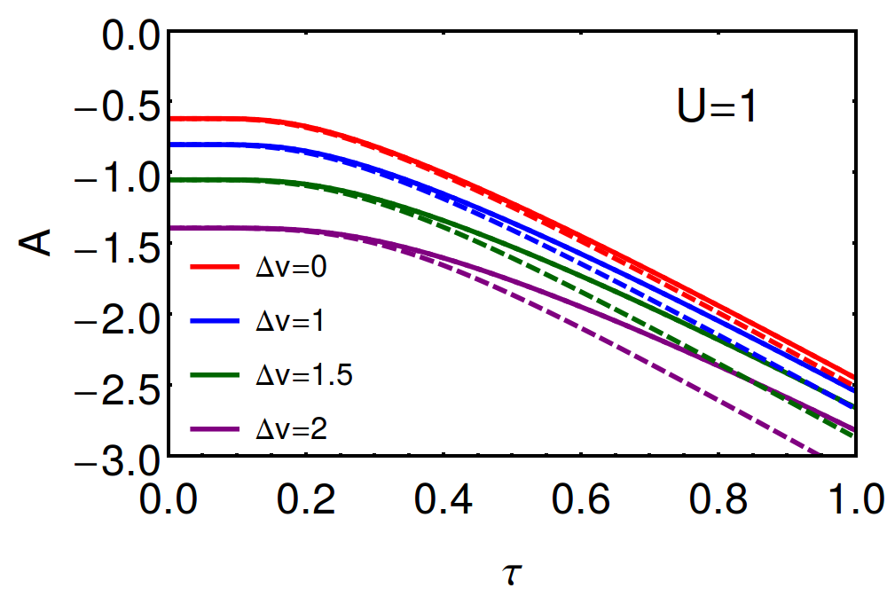
Figure 1: Free energy for different values of $\Delta v$. Solid lines are exact, dashed lines are the zero-temperature XC approximation (ZTA), evaluated on the self-consistent thermal density.

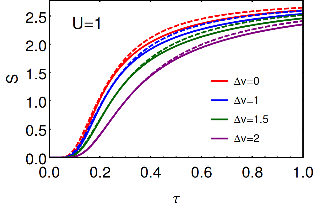
Figure 2: Exact entropy (solid) and self-consistent Kohn-Sham entropy (dashed) for different values of $\Delta v$. All curves approach $4\log 2$.

In Fig. 1 and 2, we plot the free energy and entropy as a function of temperature for several different values of $\Delta v$. For the free energy we include curves for the zero-temperature approximation and for the entropy we include the self-consistent Kohn-Sham entropy (both to be discussed later). In both cases we pick a system, i.e. fix $\Delta v$ and $U$ and see what happens as we heat it up. For the free energy, the values at $\tau=0$ recover the ground-state energies reported in Ref. Carrascal et al. (2015). Increasing temperature results in a decrease in free energy primarily due to the entropic term, $-\tau S$, as expected. At small temperatures there is minimal effect as seen in Fig. 2 where the entropy is small and further multiplied by a $\tau\ll 1$ when calculating $A$. However, once the system is sufficiently warm the entropy plays a much larger role. In contrast, increasing $\Delta v$ lowers the entropy since the asymmetry restricts the motion of electrons. Lastly, the entropy approaches a maximum value of $\log(16)$ for higher temperatures where 16 is the number of states in our grand canonical ensemble.

III.2 Inversion and correlation components

Next, we construct the exact KS potential as well as various energy components using the MKS approach. To begin we construct the exact occupation difference $\Delta n$ from Eq. (14). We plot the result in Fig. 3 for fixed $U$ but against $\Delta v$ and vary $\tau$. In this figure we also plot the ZTA result which will be discussed later. Increasing the temperature pushes the electrons apart, akin to repulsion. As the system heats up, $\Delta n$ becomes closer to 0 as both electrons sit on separate sites even when $\Delta v$ is large.

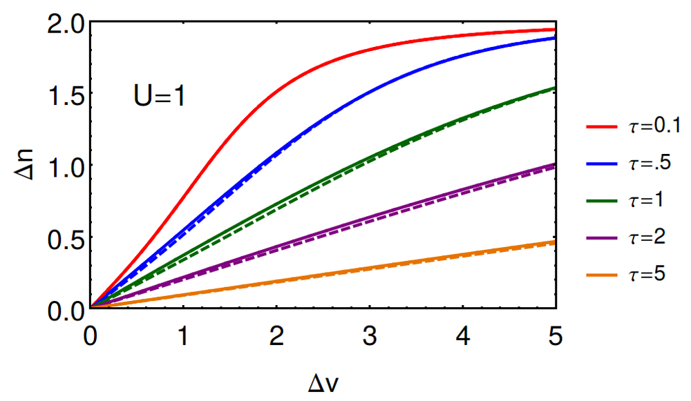
Figure 3: Densities as a function of temperature for the system of Fig. 1. Solid lines are exact, dashed lines are self-consistent KS using the ZTA.

To construct the exact MKS potential, we first give formulas for non-interacting electrons ($U=0$, a.k.a. tight-binding).

The grand canonical partition function collapses to the product

$$Z_{gc}=\prod_{i}\left(1+e^{\beta(\mu-\epsilon_{i})}\right)$$ (15)

where $\epsilon_{i}$ is the single-particle orbital energy. Eq. (12) and (13) can then be used. The entropy can also be explicitly given in terms of Fermi factors,

$$S_{\scriptscriptstyle\rm S}=-\sum_{i}f_{i}\log(f_{i})+(1-f_{i})\log(1-f_{i}).$$ (16)

where $f_{i}=(1+e^{\beta(\epsilon_{i}-\mu)})^{-1}$. The Kohn-Sham entropy is calculated in Fig. 2 where the Fermi factors are calculated from self-consistently solving the MKS equations (see below).

To construct the MKS system for the Hubbard dimer within SOFT, we simply repeat the exact calculation with $U=0$, i.e., a tight-binding dimer. We find:

$$\Delta n=-2\sin\phi\tanh\alpha$$ (17)

where $\alpha=(4\tau\cos\phi)^{-1}$, $\sin\phi=x/{\sqrt{1+x^{2}}}$, $\tau$ is in units of $2\,t$, and $x=\Delta v_{\scriptscriptstyle\rm S}/2\,t$. To perform the inversion for a given density from the many-body problem, we perform a binary search at the given temperature on Eq. (17) to find $\Delta v_{\scriptscriptstyle\rm S}(\Delta n)$, the exact KS site-potential difference that yields the required occupation density. The exact $\Delta v_{\scriptscriptstyle\rm XC}$ for the given $\Delta n$ is then found by subtracting off the other potential contributions, i.e., $\Delta v$ and $\Delta v_{\scriptscriptstyle\rm H}$. The Hartree energy (in the standard DFT definitionPribram-Jones et al. (2014b)) for this model is

$$U_{\scriptscriptstyle\rm H}(\Delta n)=U\left(1+\frac{\Delta n^{2}}{4}\right),$$ (18)

and the Hartree potential is simply

$$v_{\scriptscriptstyle\rm H}(\Delta n)=U\Delta n/2$$ (19)

and both functionals are temperature-independent. For two unpolarized electrons, $E_{\scriptscriptstyle\rm X}=-U_{\scriptscriptstyle\rm H}/2$ at all temperaturesPribram-Jones et al. (2014a), and so is also independent of $\tau$. The thermal MKS hopping energy is just that of this tight-binding problem:

$$T_{\scriptscriptstyle\rm S}^{\rm\tau}(\Delta n)/(2t)=\Delta n/x(\Delta n)$$ (20)

and the tight-binding MKS entropy is

$$S_{\scriptscriptstyle\rm S}^{\rm\tau}(\Delta n)=4\log\left\{2\cosh\alpha\right\}-4\alpha\tanh\alpha$$ (21)

With these simple results, we can now extract the correlation free energy for this problem as

$$A_{\scriptscriptstyle\rm C}^{\rm\tau}=(T^{\rm\tau}-T_{\scriptscriptstyle\rm S}^{\rm\tau})-\tau(S^{\rm\tau}-S_{\scriptscriptstyle\rm S}^{\rm\tau})+(V_{\rm ee}^{\rm\tau}-U_{\scriptscriptstyle\rm HX})$$ (22)

where $T^{\rm\tau}$, $S^{\rm\tau}$, and $V_{\rm ee}^{\rm\tau}$ are calculated from the many-body problem via eqs. (14), (12), and (14). Since $A_{\scriptscriptstyle\rm X}^{\rm\tau}$ is trivial and has no thermal contribution for our system, $A_{\scriptscriptstyle\rm C}^{\rm\tau}$ is what we study, and we know of no other exact calculation of this quantity for a finite system.

IV Numerical results

Performing the inversion to explicitly analyze the MKS potential shows how the features of interactions are built into the non-interacting potentialThiele et al. (2008); Coe et al. (2009); Nielsen et al. (2013). The crux of the MKS approach is that we capture the effects of interactions through the modified external potential $\Delta v_{\scriptscriptstyle\rm S}$. For example, interaction causes the dimer occupations to be more symmetric, thus $\Delta v_{\scriptscriptstyle\rm S}<\Delta v$ for a MB system with $U>0$. Similarly, for any given density both potentials, $\Delta v$ and $\Delta v_{\scriptscriptstyle\rm S}$, increase with temperature to counteract thermal effects pushing the system towards symmetry. But even in this simple model, there is a vast parameter space to be explored as, choosing $2\,t=1$, we can vary $U$, $\Delta v$, $\tau$, and $\langle N\rangle$. We focus on $\langle N\rangle=2$, and the weakly-correlated and low temperature corner of our parameter space: $U,\tau<1$. In particular, we avoid warming our model so much that properties are strongly influenced by the very limited Hilbert space. Specifically, we check that the system is not too hot by computing the occupations of all the states in the grand canonical ensemble. We test this in the symmetric case because it is most prone to overheating since asymmetry competes against thermal effects. For $U=1$, uniform occupation of all states does not occur until $\tau\gg 8$ and appreciable uniformity does not start to arise until $\tau\approx 4$. Thus our results are not limited by the top of our Hilbert space.

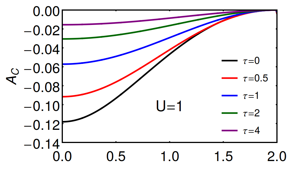
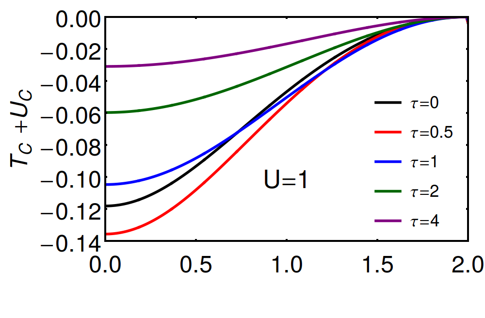
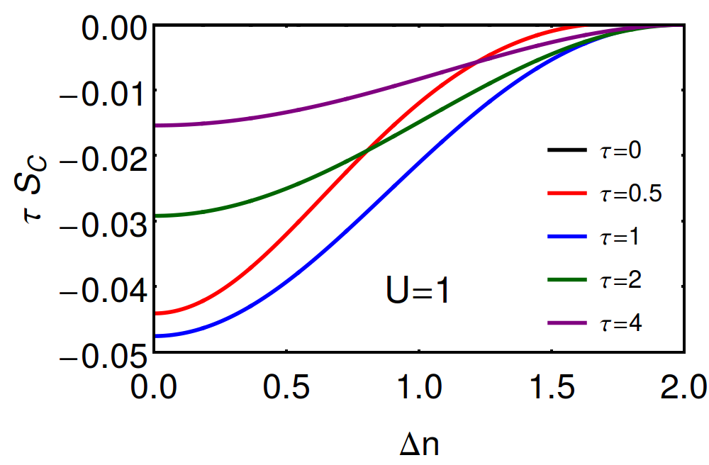
Figure 4: Panel 1: Correlation free energy functional for various temperatures. Panel 2: Sum of kinetic and potential energy functional for various temperatures. Panel 3: Entropic correlation functional for various temperatures.

We can calculate all the individual contributions to the correlation free energy by subtracting MKS quantities from their physical counterparts. These are the energy differences appearing in Eq. (22):

$$T_{\scriptscriptstyle\rm C}^{\rm\tau}=T^{\rm\tau}-T_{\scriptscriptstyle\rm S}^{\rm\tau},~{}~{}~{}S_{\scriptscriptstyle\rm C}^{\rm\tau}=S^{\rm\tau}-S_{\scriptscriptstyle\rm S}^{\rm\tau},~{}~{}~{}~{}U_{\scriptscriptstyle\rm C}^{\rm\tau}=V_{\rm ee}^{\rm\tau}-U_{\scriptscriptstyle\rm HX}.$$ (23)

The kentropic correlation is $K_{\scriptscriptstyle\rm C}=T_{\scriptscriptstyle\rm C}-\tau\,S_{\scriptscriptstyle\rm C}$ and plays a key role in thermal DFTPittalis et al. (2011). In Fig. 4, we plot the exact correlation free energy functional, the sum of kinetic and potential correlation functional, and lastly the entropic correlation functional all for various temperatures. By fixing $U$ and $\tau$ and plotting versus $\Delta n$, we analyze the correlation as a density functional, i.e. we are no longer looking at a fixed system and instead are looking at the underlying structure of how thermal DFT behaves.

We see that the correlation free energy is always negative, the kentropic contribution is always positive (not shown), and the potential contribution is always negative. These are consistent with conditions on the correlationPittalis et al. (2011). This is the first exact investigation of those inequalities. The correlation free energy, $A_{\scriptscriptstyle\rm C}^{\rm\tau}$, always decreases with temperature at $U=1$, even though the components do not behave that way at small temperature. $T_{\scriptscriptstyle\rm C}+U_{\scriptscriptstyle\rm C}$ and $\tau S_{\scriptscriptstyle\rm C}$ also decrease for all densities at larger temperature just like $A_{\scriptscriptstyle\rm C}$. In this regime, thermal effects dominate over interactions, resulting in the interacting system and the non-interacting system having similar energy components and thus relatively smaller correlation. But for small temperature, i.e. $\tau<1$ when $U=1$, the MKS quantities are furthest from the exact system since neither effect dominates and this results in an even larger difference between the two systems than at $\tau=0$. Overall we see the same behavior as in the ground-state caseCarrascal et al. (2015) – correlation decreases as our system becomes more asymmetric. If the electrons are completely pinned on the lower site then there is no motion, the interaction is completely described by the Hartree, and there is only one entropic conformation.

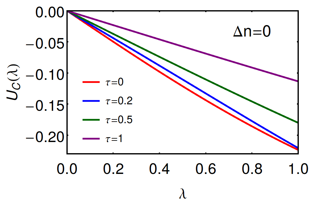
Figure 5: Adiabatic connection integrand for the symmetric dimer at several different temperatures.

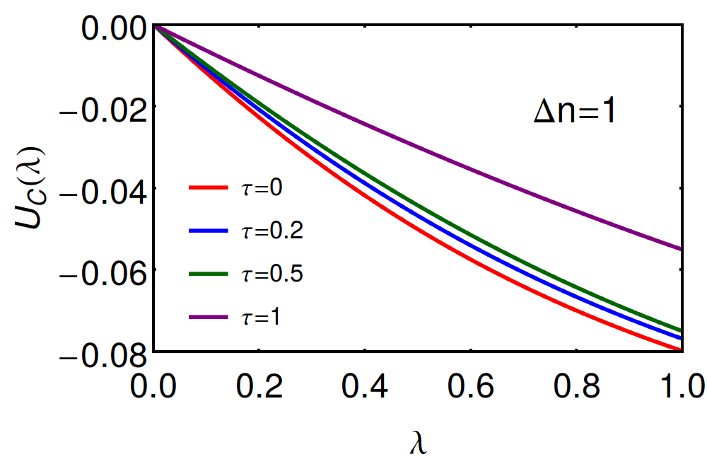
Figure 6: Same as Fig. 5, except $\Delta n=1$.

Next, we consider the adiabatic connection formulaLangreth and Perdew (1975); Gunnarsson and Lundqvist (1976) that has proven useful in studying and improving density functional approximations. The ground-state version was calculated for the Hubbard dimer in Fig. 21 of Ref. Carrascal et al. (2015). An alternative version, called the thermal connection formula, was derived in Ref. PB1 (2015), but that flavor relies on relating the coupling-constant to coordinate scaling. Such a procedure applies to continuum models, but not lattices. So we use the traditional version here, applied to finite temperaturePittalis et al. (2011):

$$A_{\scriptscriptstyle\rm C}^{\rm\tau}[n]=\int_{0}^{1}\frac{d\lambda}{\lambda}U_{\scriptscriptstyle\rm C}^{\rm\tau,\lambda}[n]$$ (24)

where $\lambda$ is a coupling constant inserted in front of $\hat{V}_{\rm ee}$ in the Hamiltonian, but (unlike regular many-body theory) the density is held fixed during the variation. Here $U_{\scriptscriptstyle\rm C}^{\rm\tau,\lambda}$ is the potential correlation energy at coupling constant $\lambda$, which, for our model, is obtained by replacing $U$ with $\lambda U$. In Fig. 5, for the symmetric case, turning on temperature clearly reduces both the magnitude of the correlation and the degree of static correlation, as judged by the initial slope of the curves. Fig. 6 shows this result remains true beyond the symmetric case.

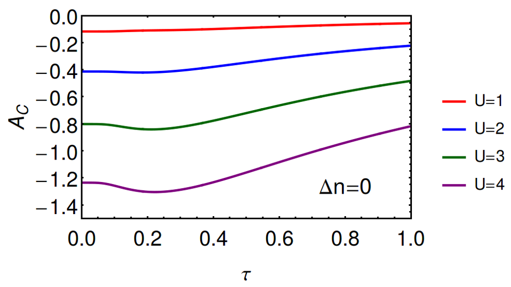
Figure 7: Correlation free energy for the symmetric case with increasing values of $U$ ranging from weak to strong correlation.

In Fig. 7, we repeat the $A_{\scriptscriptstyle\rm C}^{\rm\tau}$ curves of Fig. 4 but now for fixed $\Delta n=0$ and increasing $U$. We start with the $U=1$ from earlier and increase into the strongly correlated regime. The curves show a minimum at about $\tau=0.25$, particularly in $U=3$ and 4. Thus the derivative with respect to temperature can be negative, and this does not happen even if we look closely at $U=1$. Thus the correlation free energy is not generally monotonically decreasing in magnitude and the correlation energy is not bounded by the $\tau=0$ value.

V Zero-temperature approximation

In this section, we explore the effects of making the zero-temperature approximation (ZTA), in which thermal contributions are ignored (Eq. (10)). We use the (essentially) exact parametrization of the ground-state XC energy of the Hubbard dimer of Eq. (108) of Ref. Carrascal et al. (2015). This substitution is made in the calculation of the total free energy and in the MKS equations via the calculation of the XC potential, Eq. (6). We return to Fig. 1, where we also plot the free energy in the ZTA by replacing $A_{\scriptscriptstyle\rm C}^{\tau}(\Delta n)$ with $E_{\scriptscriptstyle\rm C}(\Delta n)$, evaluated on the self-consistent $\Delta n$. We see that the error of ZTA is extremely small for $\tau\lesssim 0.5$. Moreover, trends are very well reproduced by the ZTA values, and fractional errors shrink for large $\tau$. This suggests that free energies in such calculations may be reliable depending, of course, on the precision needed in a given calculation. The errors grow most rapidly with $\tau$ when the dimer is asymmetric. Thermal effects push the electrons apart, making the density more symmetric, in direct competition with $\Delta v$. For larger $\Delta n$, there is a larger error in ignoring thermal effects. Note that since we have only two electrons, our model is a worst case scenario. In many simulations, there are more valence electrons per site, and (exchange-)correlation components are a much smaller fraction of the total energy. In a realistic DFT calculation, the error made by approximating the ground-state functional would likely be much larger than the error due to the lack of temperature-dependenceSjostrom and Daligault (2014).

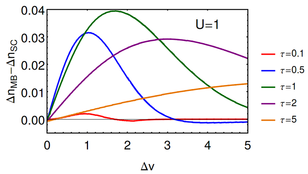
Figure 8: Error in ZTA densities of Fig. 3, density from self-consistent MKS subtracted from exact density.

However, this is only part of the story. Real thermal DFT calculations are performed self-consistently within ZTA. Then both the density and MKS orbitals are often used to calculate response properties (usually on the MKS orbitals)Silvestrelli (1999); Silvestrelli et al. (1997); Recoules et al. (2002); Clérouin et al. (2005); Desjarlais et al. (2002); Recoules et al. (2003); Desjarlais (2005); Recoules et al. (2009); Plagemann et al. (2012). In Fig. 3, we compare the self-consistent density obtained using Eq. (4) through Eq. (7). In Fig. 8, we plot the differences. We see that the maximum errors in the density are small. At first they grow with small temperature but quickly start to lessen as temperature increases which will be further explained below. As $\Delta v$ gets large the error goes to zero since the asymmetry dominates over thermal effects.

In terms of Fig. 4, the ZTA consists of approximating each of the curves by the corresponding black one. Because all correlation components tend to vanish with increasing temperature, while the total free energy grows in magnitude, the small error made in the ZTA becomes less relevant with increasing temperature. Specifically, we can analyze the symmetric case where correlation effects are at their strongest. At $\tau=0$ correlation is about 20% of the total energy but when the system is at $\tau=1$ correlation is roughly 2.5% of the total free energy. More importantly this is due to the total energy magnitude going up by a factor of 5 and the correlation only decreasing by a factor of 2. This explains the small errors in the ZTA free energies of Fig. 1 and the behavior of the self-consistent ZTA densities of Fig. 8. Note that the temperatures need not be so high as to make the density uniform (i.e., symmetric). Fig. 3 shows that, even for the temperature at which density differences can be largest ($\tau=1$), the density difference can remain substantial as the temperature increases, if the inhomogeneity ($\Delta v$) is large enough.

VI Conclusions

In summary, we have solved the simplest possible non-trivial system at finite temperature exactly, both for the many-body case and within MKS density functional theory. We have produced the first exact plots of MKS quantities and the ZTA approximation for a finite system (albeit one with a limited Hilbert space). When the system is weakly correlated system at low to moderate temperatures, the neglect of thermal contributions to the exchange-correlation functional has relatively little effect on the calculated free energies and even less on the self-consistent densities. Present limitations of ground-state approximations, such as their inability to treat strongly correlated systems, are likely the greatest source of error in these calculations. Future work will explore other quantities of interest within thermal DFT and will analyze the ZTA more deeply.

Appendix A Energies and Densities for all States

Here we list all the total energies, energy components, and density components for all particle numbers so that all the relevant ensemble averages of Eq. (14) can be reconstructed. We begin with the energies

$$E_{i}(4-N) = (2-N)U+E_{i}(N)~{}~{}~{}~{}~{}~{}N=0\rm{\textendash}4,$$

$$E_{0}(0) = 0,$$

$$E_{0,1}(1) = \mp\sqrt{(2\,t)^{2}+\Delta v^{2}}/2,$$

$$E_{i}(2) = \frac{2\,U}{3}-\frac{2\,r}{3}\cos(\theta+\frac{2\pi}{3}(i+1))~{}~{}~{}~{}~{}~{}i=0,1,2,$$

$$E_{i}(2) = 0,~{}~{}~{}~{}~{}~{}i=3,4,5,$$

where

$$r = \sqrt{3((2\,t)^{2}+\Delta v^{2})+U^{2}},$$

$$\theta = \frac{1}{3}\arccos\left[\frac{9U(\Delta v^{2}-2\,t^{2})-U^{3}}{(3((2\,t)^{2}+\Delta v^{2})+U^{2})^{3/2}}\right].$$

$E_{1}(2)$ and $E_{2}(2)$ are both positive and should be ordered 4 and 5 instead. However the three triplets, i.e. the three zero-energy states, give only zero values in the later expectation values, so for notational convenience we order the non-zero 2-particle states 0, 1, and 2 instead of 0, 4, and 5. These energies were used to construct $Z_{gc}$ in Eq. (11) of the main text.

Next are the expectation values needed to construct the three different ensemble averages of interest, $T$, $V_{\rm ee}$, and $\Delta n$ ($V_{\rm ext}$ is unnecessary since it is trivially $\Delta v\Delta n/2$):

$$T_{i}(4-N) = T_{i}(n)~{}~{}~{}~{}~{}~{}N=0\rm{\textendash}4$$

$$T_{0,1}(1) = \mp\frac{t}{\sqrt{(2\,t)^{2}+\Delta v^{2}}},$$

$$T_{i}(2) = (\beta_{i}^{+}+\beta_{i}^{-})^{2}/E_{i}(2)~{}~{}~{}~{}~{}~{}i=0,1,2,$$

$$V_{\rm{ee},i}(4-N) = (2-N)U+V_{\rm{ee},i}(N)~{}~{}~{}~{}~{}~{}N=0\rm{\textendash}4,$$

$$V_{\rm{ee},0,1}(1) = 0,$$

$$V_{\rm{ee},i}(2) = U((\beta_{i}^{+})^{2}+(\beta_{i}^{-})^{2})~{}~{}~{}~{}~{}~{}i=0,1,2,$$

$$\Delta n_{i}(4-N) = \Delta n_{i}(N)~{}~{}~{}~{}~{}~{}N=0\rm{\textendash}4,$$

$$\Delta n_{0,1}(1) = \mp\frac{2\Delta v}{\sqrt{(2\,t)^{2}+\Delta v^{2}}},$$

$$\Delta n_{i}(2) = 2((\beta_{i}^{-})^{2}-(\beta_{i}^{+})^{2})~{}~{}~{}~{}~{}~{}i=0,1,2,$$

and all the 0-particle terms are 0. The $\beta^{\pm}$’s are from the $N=2$ wavefunction:

$$|\Psi_{i}(N)\rangle=\alpha_{i}(N)(|12\rangle+|21\rangle)+\beta_{i}^{+}(N)|11\rangle+\beta_{i}^{-}(N)|22\rangle$$

with

$$\alpha_{i} = \frac{2\,t\,(E_{i}(2)-U)}{c_{i}E_{i}(2)},~{}~{}\beta_{i}^{\pm}=\frac{U-E_{i}(2)\pm\Delta v}{c_{i}},$$

$$c_{i} = \sqrt{2(\Delta v^{2}+(E_{i}(2)-U^{2})^{2}(1+(2\,t/E_{i}(2))^{2})}.$$

The ket $|ij\rangle$ signifies an electron at site $i$ and site $j$. These expectation values were used with Eq. (14) to construct the densities and energy components shown in the figures.

References

- Hohenberg and Kohn (1964) P. Hohenberg and W. Kohn, “Inhomogeneous electron gas,” Phys. Rev. 136, B864–B871 (1964).
- Graziani et al. (2014) Frank Graziani, Michael P. Desjarlais, Ronald Redmer, and Samuel B. Trickey, eds., Frontiers and Challenges in Warm Dense Matter, Lecture Notes in Computational Science and Engineering, Vol. 96 (Springer International Publishing, 2014).
- of Energy (2009) U.S. Department of Energy, Basic Research Needs for High Energy Density Laboratory Physics: Report of the Workshop on High Energy Density Laboratory Physics Research Needs, Tech. Rep. (Office of Science and National Nuclear Security Administration, 2009).
- Mattsson and Desjarlais (2006) Thomas R. Mattsson and Michael P. Desjarlais, “Phase diagram and electrical conductivity of high energy-density water from density functional theory,” Phys. Rev. Lett. 97, 017801 (2006).
- Lorenzen et al. (2009) Winfried Lorenzen, Bastian Holst, and Ronald Redmer, “Demixing of hydrogen and helium at megabar pressures,” Phys. Rev. Lett. 102, 115701 (2009).
- Knudson et al. (2015a) M. D. Knudson, M. P. Desjarlais, A. Becker, R. W. Lemke, K. R. Cochrane, M. E. Savage, D. E. Bliss, T. R. Mattsson, and R. Redmer, “Direct observation of an abrupt insulator-to-metal transition in dense liquid deuterium,” Science 348, 1455–1460 (2015a).
- Knudson and Desjarlais (2009) M. D. Knudson and M. P. Desjarlais, “Shock compression of quartz to 1.6 TPa: Redefining a pressure standard,” Phys. Rev. Lett. 103, 225501 (2009).
- Knudson et al. (2015b) M. D. Knudson, M. P. Desjarlais, and A. Pribram-Jones, “Adiabatic release measurements in aluminum between 400 and 1200 gpa: Characterization of aluminum as a shock standard in the multimegabar regime,” Phys. Rev. B 91, 224105 (2015b).
- Holst et al. (2008) Bastian Holst, Ronald Redmer, and Michael P. Desjarlais, “Thermophysical properties of warm dense hydrogen using quantum molecular dynamics simulations,” Phys. Rev. B 77, 184201 (2008).
- Kietzmann et al. (2008) André Kietzmann, Ronald Redmer, Michael P. Desjarlais, and Thomas R. Mattsson, “Complex behavior of fluid lithium under extreme conditions,” Phys. Rev. Lett. 101, 070401 (2008).
- Root et al. (2010) Seth Root, Rudolph J. Magyar, John H. Carpenter, David L. Hanson, and Thomas R. Mattsson, “Shock compression of a fifth period element: Liquid xenon to 840 GPa,” Phys. Rev. Lett. 105, 085501 (2010).
- Smith et al. (2014) R F Smith, J H Eggert, R Jeanloz, T S Duffy, D G Braun, J R Patterson, R E Rudd, J Biener, A E Lazicki, A V Hamza, J Wang, T Braun, L X Benedict, P M Celliers, and G W Collins, “Ramp compression of diamond to five terapascals,” Nature 511, 330–3 (2014).
- Dharma-Wardana and Taylor (1981) MWC Dharma-Wardana and R Taylor, “Exchange and correlation potentials for finite temperature quantum calculations at intermediate degeneracies,” Journal of Physics C: Solid State Physics 14, 629 (1981).
- Perrot and Dharma-wardana (1984) Francois Perrot and M. W. C. Dharma-wardana, “Exchange and correlation potentials for electron-ion systems at finite temperatures,” Phys. Rev. A 30, 2619–2626 (1984).
- Perdew et al. (1996) John P. Perdew, Kieron Burke, and Matthias Ernzerhof, “Generalized gradient approximation made simple,” Phys. Rev. Lett. 77, 3865–3868 (1996), ibid. 78, 1396(E) (1997).
- Mermin (1965) N. D. Mermin, “Thermal properties of the inhomogenous electron gas,” Phys. Rev. 137, A: 1441 (1965).
- Kohn and Sham (1965) W. Kohn and L. J. Sham, “Self-consistent equations including exchange and correlation effects,” Phys. Rev. 140, A1133–A1138 (1965).
- Atzeni and Meyer-ter Vehn (2004) S. Atzeni and J. Meyer-ter Vehn, The Physics of Inertial Fusion: Beam-Plasma Interaction, Hydrodynamics, Hot Dense Matter (Clarendon Press, 2004).
- Pribram-Jones et al. (2014a) Aurora Pribram-Jones, Stefano Pittalis, E.K.U. Gross, and Kieron Burke, “Thermal density functional theory in context,” in Frontiers and Challenges in Warm Dense Matter, Lecture Notes in Computational Science and Engineering, Vol. 96, edited by Frank Graziani, Michael P. Desjarlais, Ronald Redmer, and Samuel B. Trickey (Springer International Publishing, 2014) pp. 25–60.
- Karasiev et al. (2012) Valentin V. Karasiev, Travis Sjostrom, and S. B. Trickey, “Comparison of density functional approximations and the finite-temperature hartree-fock approximation in warm dense lithium,” Phys. Rev. E 86, 056704 (2012).
- Ernzerhof and Scuseria (1999) M. Ernzerhof and G. E. Scuseria, “Assessment of the Perdew–Burke–Ernzerhof exchange-correlation functional,” J. Chem. Phys 110, 5029 (1999).
- J. Paier and Kresse (2005) M. Marsman J. Paier, R. Hirschl and G. Kresse, “The perdew-burke-ernzerhof exchange-correlation functional applied to the g2-1 test set using a plane-wave basis set,” J. Chem. Phys. 122, 234102 (2005).
- O.V. Gritsenko and Baerends (1997) P.R.T. Schipper O.V. Gritsenko and E.J. Baerends, “Exchange and correlation energy in density functional theory. comparison of accurate dft quantities with traditional hartree-fock based ones and generalized gradient approximations for the molecules li2, n2, and f2,” J. Chem. Phys. 107, 5007 (1997).
- Ziesche et al. (1998) Paul Ziesche, Stefan Kurth, and John P. Perdew, “Density functionals from LDA to GGA,” Computational Materials Science 11, 122 – 127 (1998).
- S. Kurth and Blaha (1999) J.P. Perdew S. Kurth and P. Blaha, “Molecular and solid-state tests of density functional approximations: Lsd, gga’s, and meta-gga’s,” Int. J. Quantum Chem. 75, 889 (1999).
- Jain et al. (2013) Anubhav Jain, Shyue Ping Ong, Geoffroy Hautier, Wei Chen, William Davidson Richards, Stephen Dacek, Shreyas Cholia, Dan Gunter, David Skinner, Gerbrand Ceder, and Kristin A. Persson, “Commentary: The materials project: A materials genome approach to accelerating materials innovation,” APL Materials 1, – (2013).
- Filinov et al. (2001) V S Filinov, M Bonitz, W Ebeling, and V E Fortov, “Thermodynamics of hot dense h-plasmas: path integral monte carlo simulations and analytical approximations,” Plasma Physics and Controlled Fusion 43, 743 (2001).
- Schoof et al. (2011) T. Schoof, M. Bonitz, A. Filinov, D. Hochstuhl, and J.W. Dufty, “Configuration path integral monte carlo,” Contributions to Plasma Physics 51, 687–697 (2011).
- Driver and Militzer (2012) K. P. Driver and B. Militzer, “All-electron path integral monte carlo simulations of warm dense matter: Application to water and carbon plasmas,” Phys. Rev. Lett. 108, 115502 (2012).
- Brown et al. (2013) Ethan W. Brown, Bryan K. Clark, Jonathan L. DuBois, and David M. Ceperley, “Path-integral monte carlo simulation of the warm dense homogeneous electron gas,” Phys. Rev. Lett. 110, 146405 (2013).
- Schoof et al. (2015) T. Schoof, S. Groth, J. Vorberger, and M. Bonitz, “Ab Initio thermodynamic results for the degenerate electron gas at finite temperature,” Phys. Rev. Lett. 115, 130402 (2015).
- Militzer and Driver (2015) Burkhard Militzer and Kevin P. Driver, “Development of path integral monte carlo simulations with localized nodal surfaces for second-row elements,” Phys. Rev. Lett. 115, 176403 (2015).
- Groth et al. (2016) S. Groth, T. Schoof, T. Dornheim, and M. Bonitz, “Ab initio quantum monte carlo simulations of the uniform electron gas without fixed nodes,” Phys. Rev. B 93, 085102 (2016).
- Militzer (2009) B. Militzer, “Path integral monte carlo and density functional molecular dynamics simulations of hot, dense helium,” Phys. Rev. B 79, 155105 (2009).
- Vorberger and Gericke (2015) J. Vorberger and D. O. Gericke, “Ab initio approach to model x-ray diffraction in warm dense matter,” Phys. Rev. E 91, 033112 (2015).
- Driver and Militzer (2015) K. P. Driver and B. Militzer, “First-principles simulations and shock hugoniot calculations of warm dense neon,” Phys. Rev. B 91, 045103 (2015).
- Driver and Militzer (2016) K. P. Driver and B. Militzer, “First-principles equation of state calculations of warm dense nitrogen,” Phys. Rev. B 93, 064101 (2016).
- Patton et al. (1997) David C. Patton, Dirk V. Porezag, and Mark R. Pederson, “Simplified generalized-gradient approximation and anharmonicity: Benchmark calculations on molecules,” Phys. Rev. B 55, 7454–7459 (1997).
- Baerends (2001) E.J. Baerends, “Exact exchange-correlation treatment of dissociated h2 in density functional theory,” Phys. Rev. Lett. 87, 133004 (2001).
- Carrascal et al. (2015) D J Carrascal, J Ferrer, J C Smith, and K Burke, “The hubbard dimer: a density functional case study of a many-body problem,” Journal of Physics: Condensed Matter 27, 393001 (2015).
- Pribram-Jones et al. (2014b) A. Pribram-Jones, Z.-H. Yang, J. R. Trail, K. Burke, R. J. Needs, and C. A. Ullrich, “Excitations and benchmark ensemble density functional theory for two electrons,” J. Chem. Phys. 140, 18A541 (2014b).
- Schönhammer et al. (1995) K. Schönhammer, O. Gunnarsson, and R. M. Noack, “Density-functional theory on a lattice: Comparison with exact numerical results for a model with strongly correlated electrons,” Phys. Rev. B 52, 2504–2510 (1995).
- Beale (2011) Paul D. Beale, R.K. Pathria, Statistical Mechanics, 3rd ed. (Academic Press, 2011).
- Shiba (1972) Hiroyuki Shiba, “Thermodynamic properties of the one-dimensional half-filled-band hubbard model. ii application of the grand canonical method,” Progress of Theoretical Physics 48, 2171–2186 (1972).
- Thiele et al. (2008) M. Thiele, E. K. U. Gross, and S. Kümmel, “Adiabatic approximation in nonperturbative time-dependent density-functional theory,” Phys. Rev. Lett. 100, 153004 (2008).
- Coe et al. (2009) J. P. Coe, K. Capelle, and I. D’Amico, “Reverse engineering in many-body quantum physics: Correspondence between many-body systems and effective single-particle equations,” Phys. Rev. A 79, 032504 (2009).
- Nielsen et al. (2013) S. E. B. Nielsen, M. Ruggenthaler, and R. van Leeuwen, “Many-body quantum dynamics from the density,” EPL (Europhysics Letters) 101, 33001 (2013).
- Pittalis et al. (2011) S. Pittalis, C. R. Proetto, A. Floris, A. Sanna, C. Bersier, K. Burke, and E. K. U. Gross, “Exact conditions in finite-temperature density-functional theory,” Phys. Rev. Lett. 107, 163001 (2011).
- Langreth and Perdew (1975) D.C. Langreth and J.P. Perdew, “The exchange-correlation energy of a metallic surface,” Solid State Commun. 17, 1425 (1975).
- Gunnarsson and Lundqvist (1976) O. Gunnarsson and B.I. Lundqvist, “Exchange and correlation in atoms, molecules, and solids by the spin-density-functional formalism,” Phys. Rev. B 13, 4274 (1976).
- PB1 (2015) “Connection formula for thermal density functional theory,” Phys. Rev. (2015), submitted.
- Sjostrom and Daligault (2014) Travis Sjostrom and Jérôme Daligault, “Gradient corrections to the exchange-correlation free energy,” Phys. Rev. B 90, 155109 (2014).
- Silvestrelli (1999) Pier Luigi Silvestrelli, “No evidence of a metal-insulator transition in dense hot aluminum: A first-principles study,” Phys. Rev. B 60, 16382–16388 (1999).
- Silvestrelli et al. (1997) Pier Luigi Silvestrelli, Ali Alavi, and Michele Parrinello, “Electrical-conductivity calculation in ab initio simulations of metals:application to liquid sodium,” Phys. Rev. B 55, 15515–15522 (1997).
- Recoules et al. (2002) Vanina Recoules, Patrick Renaudin, Jean Clérouin, Pierre Noiret, and Gilles Zérah, “Electrical conductivity of hot expanded aluminum: Experimental measurements and ab initio calculations,” Phys. Rev. E 66, 056412 (2002).
- Clérouin et al. (2005) Jean Clérouin, Patrick Renaudin, Yann Laudernet, Pierre Noiret, and Michael P. Desjarlais, “Electrical conductivity and equation-of-state study of warm dense copper: Measurements and quantum molecular dynamics calculations,” Phys. Rev. B 71, 064203 (2005).
- Desjarlais et al. (2002) M. P. Desjarlais, J. D. Kress, and L. A. Collins, “Electrical conductivity for warm, dense aluminum plasmas and liquids,” Phys. Rev. E 66, 025401 (2002).
- Recoules et al. (2003) Vanina Recoules, Jean Clérouin, P Renaudin, P Noiret, and Gilles Zérah, “Electrical conductivity of a strongly correlated aluminium plasma,” Journal of Physics A: Mathematical and General 36, 6033 (2003).
- Desjarlais (2005) M. P. Desjarlais, “Density functional calculations of the reflectivity of shocked xenon with ionization based gap corrections,” Contributions to Plasma Physics 45, 300–304 (2005).
- Recoules et al. (2009) Vanina Recoules, Flavien Lambert, Alain Decoster, Benoit Canaud, and Jean Clérouin, “Ab Initio determination of thermal conductivity of dense hydrogen plasmas,” Phys. Rev. Lett. 102, 075002 (2009).
- Plagemann et al. (2012) K.-U. Plagemann, P. Sperling, R. Thiele, M. P. Desjarlais, C. Fortmann, T. Döppner, H. J. Lee, S. H. Glenzer, and R. Redmer, “Dynamic structure factor in warm dense beryllium,” New Journal of Physics 14, 055020 (2012).