The paradox of controlling complex networks: control inputs versus energy requirement

Abstract

One of the most challenging problems in complex dynamical systems is to control complex networks. In previous frameworks based on the structural or the exact controllability theories, the ability to steer a complex network toward any desired state is measured by the minimum number of required driver nodes. However, if we implement actual control by imposing input signals on the minimum set of driver nodes as determined, e.g., by the structural controllability theory, an unexpected phenomenon arises: the energy required to approach a target state with reasonable precision is often unbearably large, precluding us from achieving actual control, i.e., the designated state can not be reached in effect, especially for networks with a small number of drivers. In particular, the energy of controlling a set of networks with similar structural properties follows a fat-tail distribution, indicating the existence of networks with practically divergent energy. We aim to reconcile the paradox of controlling complex networks: optimal structural controllability versus unrealistic energy required for control. We identify fundamental structural “short boards” in complex networks that play a dominant role in the enormous energy, and offer a theoretical interpretation for the fat-tail energy distribution and simple strategies to significantly reduce the energy by imposing slightly augmented set of input signals on properly chosen nodes. Our findings indicate that, although full control can be guaranteed by the prevailing structural controllability theory, it is necessary to balance the number of driver nodes and the control energy to achieve actual control, and our results provide a framework to address this outstanding issue.

Notes on the submission history of this work: This work started in late 2012. The phenomena of power-law energy scaling and energy divergence with a single controller were discovered in 2013. Strategies to reduce and optimize control energy was articulated and tested in Spring 2014. The senior co-author (YCL) gave talks about these results at several conferences, including the NETSCI 2014 Satellite entitled “Controlling Complex Networks” on June 2. The paper was submitted to PNAS in September 2014 and was turned down. It was revised and submitted to PRX in early 2015 and was rejected. After that it was revised and submitted to Nature Communications in May 2015 and again was turned down.

I Introduction

The past fifteen years have witnessed tremendous advances in our understanding of complex networked structures in various natural, social, and technological systems, as well as the dynamical processes taking place on themWatts and Strogatz (1998); Barabási and Albert (1999); Albert et al. (1999); L. A. N. et al. (2000); Albert et al. (2000); Cohen et al. (2000); Jeong et al. (2001); Pastor-Satorras and Vespignani (2001); Newman et al. (2002); Albert and Barabási (2002); Newman (2003); Palla et al. (2005); Boccaletti et al. (2006); Caldarelli (2007); Nagy et al. (2010); Fortunato (2010). The significant issue of control arises naturally, but this remains to be outstanding and extremely challenging, since nonlinear dynamical processes generally take place on complex networks. Control of nonlinear dynamics, especially when chaos is present, can be done but only for low-dimensional systems Ott et al. (1990); Boccaletti et al. (2000). Despite the development of nonlinear control methods Slotine and Li (1991); Wang and Chen (2002); Wang and Slotine (2005); Sorrentino et al. (2007); Yu et al. (2009); Rahmani et al. (2009) in certain particular situations such as consensus Egerstedt et al. (2012), communication Kelly et al. (1998); Chiang et al. (2007), traffic Srikant (2004) and device networks Luenberger (1979); Slotine and Li (1991), a general framework of controlling complex nonlinear-dynamical networks has yet to be developed. A natural approach is to reduce the problem to controlling complex networks with linear dynamics based on traditional frameworks from control engineering Kalman (1963); Lin (1974); Shields and Pearson (1975); Reinschke and Wiedemann (1997); Sontag (1998).

In the past a few years, great progress was made toward understanding the linear controllability of complex networks in terms of the fundamental issue of the minimum number of driver nodes required to steer the whole network system from an arbitrarily initial state to an arbitrarily final state in finite time Lombardi and Hörnquist (2007); Liu et al. (2011); Wang et al. (2012); Nepusz and Vicsek (2012); Yan et al. (2012); Liu et al. (2012); Nacher and Akustu (2012). In particular, Liu et al. successfully adopted the classic structural controllability theory developed by Lin Lin (1974) to complex networks of various topologies Liu et al. (2011), for which the traditional Kalman’s rank condition Kalman (1963) is difficult to be applied Lombardi and Hörnquist (2007). The ground breaking results show that, the structural controllability of a directed network can be assessed by using the maximum matching Hopcroft and Karp (1973); Zhou and Ou-Yang (2003); Zdeborová and Mézard (2006) algorithm. The effects of the density of in/out degree nodes were incorporated into the structural controllability framework Menichetti et al. (2014), which has also been applied to protein interaction networks Wuchty (2014). Recently, based on the classic Popov-Belevitch-Hautus (PBH) rank condition Hautus (1969) in traditional control engineering, a variant of the structural-controllability theory, the so-called exact controllability framework, was developed Yuan et al. (2013).

For both the structural- and exact-controllability frameworks, the aim is to determine the minimum number of driver nodes, $N_{\text{D}}$, for networks of various topologies. However, we have encountered unexpected difficulties in carrying out actual control of complex networks by using the minimum set of driver nodes as determined by the controllability frameworks. This concerns effectively the issue of guiding the network system to approach a final state with acceptable proximity error. In particular, given an arbitrary complex network, once $N_{\text{D}}$ is determined, we can calculate the specific control signals by using the standard linear systems theory Rugh (1996) and apply them at various unmatched nodes. A surprising finding is that, quite often, the actual control of the system is difficult to be achieved computationally in the sense that in any finite time, it is not possible to drive the system from an arbitrary initial state to an arbitrary final state, i.e., the actual state the system finally reaches is unreasonably far from the designated one. This difficulty in realizing actual control, which has not been formerly addressed in any other works, persists for a large number of model and real-world networks, prompting us to study if the developed controllability frameworks can ensure actual control with given finite computational precision and, more importantly, to consider the issue of control energy.

In this paper, we investigate the issue of control energy in the framework of structural controllability theory. We find that, the energy required to steer a system from a specific initial state to a target state in finite time follows a fat-tail distribution, indicating the existence of extraordinarily high energy requirement. In extreme but not uncommon cases, the energy is practically divergent. This phenomenon signifies the emergence of a paradox in controlling complex networks: although a small fraction of driver nodes can guarantee full control of the network system mathematically, the energy required to achieve control is often unbearable. We resolve the paradox by presenting the idea of control chains, in which the fat-tail distribution of the energy can be derived as a key structural feature. The theory of control chains enables us to offer simple strategies to significantly reduce the control energy through small augmentation of the number of control signals beyond $N_{\text{D}}$. In this regard, the quantity $N_{\text{D}}$, on which the structural controllability theories focus, can effectively be regarded as the lower bound of the actual number of control signals required. To realize actual control of a complex network, it is imperative to find the trade-off between the number of external input signals and feasible energy consumption.

Remark. In Ref. Yan et al. (2012), partial theoretical bounds for the control energy were derived. The bounds are partial because, for example, for networks whose lower bounds can be obtained, the upper bounds typically diverge. This property of divergence was puzzling: does it mean that the actual energy required would diverge as well and, if so, can a complex network actually be controlled? The present work was largely motivated by these questions, in which we obtain a detailed understanding of the physically important issue of practical controllability of complex networks through the discovery of a general scaling law for the distribution of the energy required for control. The existence of control chain is also uncovered, enabling us to articulate practical strategies to significantly reduce the control energy.

II Control Formulation and Implementation

Optimal control energy and Gramian matrix.

To calculate the optimal energy required to control a complex network in the framework of structural controllability, we consider the standard setting of linear dynamical systems under control input Lombardi and Hörnquist (2007); Liu et al. (2011); Yuan et al. (2013):

$$\mathbf{\dot{x}}=A\mathbf{x}+B\mathbf{u},$$ (1)

where $\mathbf{x}=[x_{1}(t),\ldots,x_{N}(t)]^{T}$ is the state variable of the whole network system, the vector $\mathbf{u}=[u_{1}(t),\ldots,u_{M}(t)]^{T}$ is the control input or the set of control signals, $A=\{a_{ij}\}$ is the $N\times N$ adjacency matrix of the network, and $B=\{b_{ik}\}$ is the $N\times N_{\text{D}}$ control matrix specifying the set of “driver” nodes Liu et al. (2011), each receiving a control signal (corresponding to one component of the control vector $\mathbf{u}$). The minimum number $N_{\text{D}}$ of driver nodes to fully control a network is determined through the set of maximum matching paths Liu et al. (2011). A node is chosen to be the driver node if it is the starting point of a maximum matching path. The system is fully controlled only if each and every node is either a driver node or being driven along a maximum matching path. Optimal control of a linear network in the sense that the energy is minimized can be achieved when the input control signals $\mathbf{u}_{t}$ are chosen as Chen (1984):

$$\mathbf{u}_{t}=B^{T}\cdot e^{A^{T}(t_{\text{f}}-t)}\cdot W^{-1}\cdot(\mathbf{x}_{t_{\text{f}}}-e^{A{t_{\text{f}}}}\cdot\mathbf{x}_{0}),$$ (2)

where

$$W\equiv\int_{t_{0}}^{t_{\text{f}}}e^{A\tau}B\cdot{B^{T}}\cdot e^{A^{T}\tau}d\tau$$ (3)

is the Gramian matrix, a positive-definite and symmetric matrix Rugh (1996), which is the base to determine, quantitatively, if a system is actually controllable. In particular, the system is controllable only when $W$ is nonsingular (invertible) Rugh (1996); Chen (1984).

Given matrices $A$ and $B$, the initial and the final (target) states of the system as well as the control time $t_{\text{f}}$, the control vector $\mathbf{u}$ can be determined in a standard manner Rugh (1996) via the Gramian matrix $W$. The energy required through the control input $\mathbf{u}$ is given by Rugh (1996)

$$E(t_{\text{f}})=\int_{0}^{t_{\text{f}}}\mathbf{u}^{T}_{t}\mathbf{u}_{t}dt,$$ (4)

where control is initiated at $t=0$.

Numerical implementation of control.

We use the Erdos-Renyi (ER) type of directed random networks Erdös and Rényi (1959); Erdős and Rényi (1960) and the Barabási-Albert (BA) type of directed scale-free networks Albert and Barabási (2002) with a single parameter $P_{\text{b}}$. Specifically, for a pair of nodes $i$ and $j$ with a link, the probability that it points from the smaller-degree to the larger-degree nodes is $P_{\text{b}}$, and $1-P_{\text{b}}$ is the probability that the link points in the opposite direction (if both nodes have the same degree, the link direction is chosen randomly). (See Appendix A for analytical treatment of the in- and out-degree distributions.) To determine the set of driver nodes, we use the maximum-matching algorithm Lin (1974), which gives the control matrix $B$. For each combination of $A$ and $B$, we first randomly choose the initial and final states. We then calculate the corresponding Gramian matrix $W$ [Eq. (3)], the input signal $\mathbf{u}_{t}$ [Eq. (2)], the actual final states $\mathbf{x}_{t_{\text{f}}}^{\star}$ [Eq. (1)], and finally the control energy $E(t_{\text{f}})$ [Eq. (4)]. Repeating this process for each and every independent network realization in the ensemble entails an extensive statistical analysis of the control process.

III Resolution of control paradox and control-energy distribution

III.1 Quantification of control energy and resolution of control paradox

Mathematically, if the Gramian matrix $W$ is singular, the energy diverges. Through extensive and systematic numerical computations, we find that, even when $W$ is non-singular in the mathematical sense, for typical complex networks its condition number can be enormously large Sun and Motter (2013), making it effectively singular as any physical measurement or actual computation must be associated with a finite precision. Say in a physical experiment the precision of measurement is $\varepsilon$. In a computational implementation of control, $\varepsilon$ can be regarded as the computer round-off error. Consider the solution vector $\mathbf{X}$ of the linear equation: $W\cdot\mathbf{X}=\mathbf{Y}$, where $\mathbf{Y}$ is a known vector. Let $C_{W}$ be the condition number of $W$. The accuracy of the numerical solution of $\mathbf{X}$, denoted by $e_{X}=10^{-k}$ ($k$ is a positive integer), is bounded by the product between $C_{W}$ and $\varepsilon$ Strang (1976). We see that, if $C_{W}$ is larger than $10^{-k}/\varepsilon\equiv\bar{C}_{W}$, it is not possible to bring the system to within $10^{-k}$ of the final state, so control cannot be achieved in finite time.

For a large number of networks drawn from an ensemble of networks with a pre-defined topology, the condition numbers of their Gramian matrices are often orders of magnitude larger than $\bar{C}_{W}$ (see Fig. A1 in Appendix B1 for the relation between $C_{W}$ and $e_{X}$). For these networks, not only is the control vector unable to drive the system to the target state, but the associated energy can be extremely large. These observations suggest the following criterion to define controllability in terms of the control energy: a network is controllable with respect to a specific control setting if and only if the condition number of its Gramian matrix is less than $\bar{C}_{W}$, a critical number determined by both the measurement or computational error and the required precision of control. Quantitatively, for a given set of network parameters (hence a given network ensemble) and control setting, the probability that the condition number of the Gramian matrix is less than $\bar{C}_{W}$, $P(\bar{C}_{W})$, can effectively serve as a new type of controllability, which we name as practical controllability. Increasing the precision of the computation, e.g., by using special simulation packages with round-off error orders of magnitude smaller than that associated with the conventional double-precision computation, would convert a few uncontrollable cases into controllable ones, but vast majority of the uncontrollable cases remain unchanged.

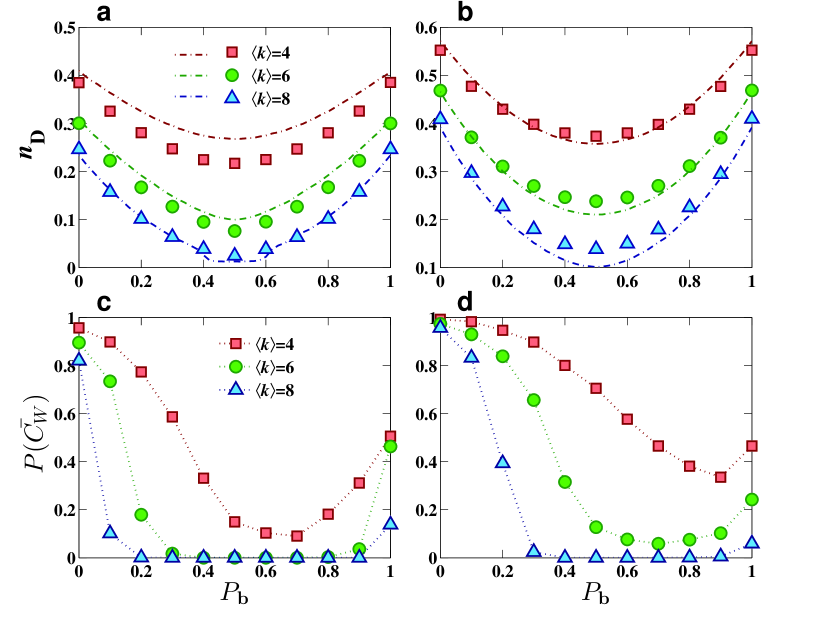
Figure 1: Structural and practical controllability measures in directed networks. Structural controllability measure $n_{\text{D}}$ versus directional edge probability $P_{\text{b}}$ for (a) ER random networks and (b) BA scale-free networks of size $N=1000$ and three values of the average degree ($\langle k\rangle=4$, $6$, and $8$). The dash-dotted lines represent the results obtained by the cavity method Liu et al. (2011), and the squares, triangles, and circles are the simulation results from the maximum matching algorithm Liu et al. (2011). (c,d) Measure of practical controllability $P(\bar{C}_{W})$ for ER random and BA scale-free networks of size $N=100$, respectively, where $P(\bar{C}_{W})$ is the probability that the condition number of the Gramian matrix is less than some physically reasonable threshold value versus $P_{\text{b}}$. Comparing (a) with (c), or (b) with (d), we observe the striking phenomenon that, in the parameter regime where the number of driver nodes is minimized so that the corresponding networks are deemed to be most structurally controllable, they are practically uncontrollable. The phenomenon persists regardless of the network size and type.

Figures 1(a-b) show the percentage of driver nodes $n_{\text{D}}\equiv N_{\text{D}}/N$ versus the directional link probability $P_{\text{b}}$. We see that $n_{\text{D}}$ is minimized for $P_{\text{b}}\approx 0.5$, indicating that, mathematically, only a few control signals are needed to control the whole network, leading to optimal structural controllability. But can practical controllability be achieved in the same parameter regime where the structural controllability is optimized?

Figure 1(c) show, for the same networks as in Fig. 1(a), the measure of control energy, i.e., the probability $P(\bar{C}_{W})$, versus the network parameter $P_{\text{b}}$. We see that, for both regimes of small and large $P_{\text{b}}$ values where the structural controllability is weak [corresponding to relatively high values of $n_{\text{D}}$ in Fig. 1(a)], the practical controllability is relatively strong. In the regime of small $P_{\text{b}}$ values, most directed links in the network point from small- to large-degree nodes. In this case, the network is more practically controllable, in agreement with intuition. The surprising result is that, in the regime of intermediate $P_{\text{b}}$ values (e.g., $P_{\text{b}}$ around 0.5) where the number of driver nodes to control the whole network is minimized so that the structural controllability is regarded as strong, the practical controllability is in fact quite weak, as the probability of the condition number being small is close to zero. For example, for $\langle k\rangle=4$, the minimum value of $P(\bar{C}_{W})$ is only about 0.1 for $P_{\text{b}}\approx 0.6$; for $\langle k\rangle=6$ and $\langle k\rangle=8$, the minimum values are essentially zero. A striking phenomenon is that the minimum value of $P(\bar{C}_{W})$ occurs in a wide range of the parameter $P_{\text{b}}$, e.g., $[0.3,0.8]$ and $[0.2,0.9]$ for $\langle k\rangle=6$ and $\langle k\rangle=8$, respectively. This indicates that the network is practically uncontrollable for most cases where the structurally controllability is deemed to be optimal. The same phenomenon holds for different network sizes (see Fig. A2 in Appendix B2). Another interesting finding in Fig. 1 is that $N_{\text{D}}$ is symmetric about $P_{\text{b}}=0.5$. However, the symmetry is broken for $P(\bar{C}_{\text{W}})$, indicating that there is no simple negative correlation between $N_{\text{D}}$ and $P(\bar{C}_{\text{W}})$. This prompts us to find more essential structural properties responsible for the smallness of $P(\bar{C}_{\text{W}})$.

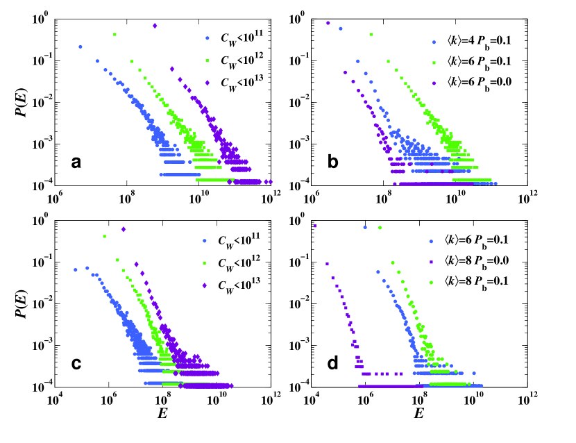
Figure 2: Distributions of control energy for practically controllable networks. (a,c) Energy distributions under different values of the threshold condition number $\bar{C}_{W}$ for $P_{\text{b}}=0.1$ and $t_{\text{f}}=1$. $\langle k\rangle=6$ for random networks (a) and $\langle k\rangle=8$ for scale-free networks (c). (b,c) Energy distributions for different values of the average degree $\langle k\rangle$ and the directional connection probability $P_{\text{b}}$ under $\bar{C}_{W}=10^{12}$ and $t_{\text{f}}=1$ for ER random and BA scale-free networks, respectively. In all cases, we observe an algebraic (power-law) scaling behavior.

III.2 Concept of control chains and distribution of control energy

Suppose the network is practically controllable so that the required control energy is not unrealistically large. For an ensemble of randomly realized network configurations with the same structural properties and for different control settings, the control energy can be regarded as a random variable. What is then its probability distribution? To gain insights, we generate directed networks with different values of $\langle k\rangle$ and $P_{\text{b}}$. We then implement the maximum matching algorithm Liu et al. (2011) to obtain the control matrix $B$ and calculate the minimum energy by using Eq. (4) for final time $t_{\text{f}}$. For each network, the initial states $\mathbf{x_{0}}$ and desired final states $\mathbf{x}_{t_{\text{f}}}$ are randomly chosen. The calculation of energy is done only for those networks with condition number smaller than $\bar{C}_{W}$, and a variety of $\bar{C}_{W}$ values are adopted. Representative results are shown in Fig. 2, where an algebraic (power-law) scaling behavior with fat tails is observed for all cases with the scaling exponent approximately equal to $1.5$. The scaling is robust against various $\bar{C}_{W}$ values [Figs. 2(a) and (c)] and network sizes (see Fig. A3 in Appendix B3). From Figs. 2(a) and (c), we see that different values of $\bar{C}_{W}$ result in different groups of practically controllable networks, and the required control energy in general increases with $\bar{C}_{W}$. In Figs. 2(b) and (d), the value of $\bar{C}_{W}$ is fixed and the control energy required is larger for larger value of $P_{\text{b}}$ as compared with the case of $P_{\text{b}}=0$. This is intuitively correct as, for $P_{\text{b}}=0$, all directed links point from small- to large-degree nodes, facilitating control of the whole network.

We develop a physical understanding of the large control energy required and also the algebraic scaling behavior in the energy distribution. To gain insights, we first consider a simple model: an unidirectional, one-dimensional (1D) string network, for which an analytic estimate of the control energy can be obtained (see Appendix C) as

$$E_{l}\approx\lambda_{{H}_{l}}^{-1},$$ (5)

where $E_{l}$ denotes the energy required to control a 1D string of length $l$ (the number of nodes on the string) and $\lambda_{{H}_{l}}$ is the smallest eigenvalue of the underlying ${H}$-matrix, denoted by ${H}_{l}$, which is related to the Gramian matrix by $H\equiv e^{-At_{\text{f}}}We^{-A^{T}t_{\text{f}}}$. The condition number of the 1D chain system increases exponentially with its length. For example, the value of $C_{W}$ of a chain of length larger than $7$ has already exceeded $\bar{C}_{W}=10^{12}$. This indicates that, even for a simple 1D chain network, the energy required for control tends to increase exponentially with the chain length. Numerical verification of Eq. (5) is presented in Figs. 3(a). Although Eq. (5) is obtained for a simple 1D chain network, we find numerically that it holds for random and scale-free network topologies (See Fig. A5 in Appendix D).

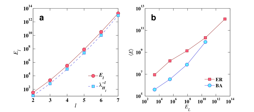
Figure 3: Relationship among 1D chain energy, the smallest eigenvalue of ${H}$-matrix, and network control energy. (a) For an 1D chain network of length $l$, energy $E_{l}$ and $\lambda_{{H}_{l}}^{-1}$ versus $l$, providing support for the analytic result Eq. (5). (b) Correlation between $\langle E\rangle$, the average of control energy for networks with the same LCC length, and $E_{L}$, the energy of a LCC with length $D_{\text{C}}=L$ ($L=3$, 4, 5, 6, and 7 for ER and $L=3$, 4, 5, and 6 for BA networks), calculated from ensembles of $10000$ networks.

The relation Eq. (5) and Fig. 3(a) provide an intuitive explanation for our finding that applying control signals to the minimum set of driver nodes calculated from the structural controllability theory typically requires enormously large energies. Under the theory of structural controllability, a network is deemed more structurally controllable if $N_{\text{D}}$ is smaller Liu et al. (2011). However, as the number of driver nodes is reduced, the length of the chain of nodes that each controller drives on average must increase, leading to an exponential growth in the control energy. In the “optimal” case of structural controllability where $N_{\text{D}}=1$ is achieved, the length of the control chain will be maximized, leading to unrealistically large control energy that prevents us from achieving actual control of the system.

The idea of exploiting the length of control chain can also be used to explain the algebraic scaling behavior in the energy consumption. As discussed, identifying maximum matching so that the network is deemed structurally controllable is independent of the control energy. However, when maximum matching is found, we can divide the whole network into $N_{\text{D}}$ control signal paths (CSPs), each being a unidirectional 1D string led by a driver node that passes the control signal onto every node along the path, as illustrated by the vertical paths in Fig. 4(a). CSPs thus provide a picture indicating how the signals from the $N_{\text{D}}$ external control inputs reach every node in the network to ensure full control (in the sense of structural controllability).

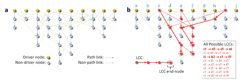
Figure 4: Schematic illustration of various concepts to characterize and understand the practical controllability of a network. (a) Control-signal paths (CSPs) of a random network obtained from maximum matching in structural controllability theory, where a control signal enters a CSP via the corresponding driver node (yellow), the starting node of the path, and goes through each matched node (blue) along the path. In this example, the network has $n_{\text{D}}=10$ CSPs of different lengths. Non-path links, links that are irrelevant to matching, are displayed in green. (d) All possible LCCs in the network. Typically there are multiple LCCs of the same length. In this example, the length of the LCCs is 4, which is defined as the control diameter of the network. Two LCCs sharing no common nodes are marked by red nodes and solid red arrows. Links belonging to other LCCs are marked by red dashed arrows. CSPs are denoted using letters $a$ to $j$ from the left to the right. Each node is specified using its path number and its position along the path sequentially from top to bottom. For example, node $e1$ is the driver node of path $e$, and node $h2$ is the node right after the driver node on path $h$. The two LCCs with solid arrows are listed in bold. Eight LCCs in the network converge to only three end-nodes, $e6$, $f5$, and $f6$ (marked by red dashed circles), leading to LCC degeneracy $m=3$. The control energy is determined by any randomly chosen $m$ LCCs among all existent ones.

We can distinguish two types of links: one along and another between the CSPs, as shown in Fig. 4(a). It may seem that the latter class are less important as the control signal and energy flow along the former set of links. However, due to coupling, a node’s dynamical state will affect all its nearest neighbors’ states which, in turn, will affect the states of their neighbors, so on, and vice versa. In principle, any driver node connects with nodes both along and outside its CSP. Correspondingly, an arbitrary node in the network is influenced by every driver node, directly through the CSP to which it belongs, or indirectly through the CSPs that it does not sit on. Intuitively, the ability of a driver node to influence a node becomes weaker as the distance between them is increased. In order to control a distant node, exponentially increased energy from the driver is needed. The chain starting from a driver node and ending at a non-driver node along their shortest path is effectively a control chain. We can define the length of the longest control chain (LCC), $D_{\text{C}}$, as the control diameter of the network, as shown in Fig. 4(b). There can be multiple LCCs. The node at the end of a LCC is most difficult to be controlled in the sense that the largest amount of control energy is required. The number $m$ of such end nodes dictates the degeneracy (multiplicity) of LCCs. An example is shown in Fig. 4(b), where we see that, although there can be multiple LCCs, the ends of them converge to only three nodes, leading to $m=3$. Since the energy required to control a 1D chain grows exponentially with its length in such a way that even one unit of increase in the length can amplify the energy by several orders of magnitude [Fig. 3(a)], the energy associated with any chain shorter than the LCC can typically be several orders of magnitude smaller than that with the LCC. Thus, the total energy is dominated by the LCCs. Due to the low value of typical $m$ (see Fig. A6 in Appendix E1), a single LCC essentially dictates the energy magnitude of the whole system. As shown in Fig. 3(b), actual network control energy shares strong positive correlation and similar magnitude to the LCC energy $E_{L}$, defined as the energy of a LCC of the corresponding network, especially for networks with long LCCs. Intuitively, the probability to form long LCCs is small. Accordingly, a longer LCC tends to have smaller value of degeneracy $m$. As a result, the longest LCCs have almost no degeneracy ($m=1$) so that they effectively rule the control energy of the whole network (see Appendix E1).

The construction in Fig. 4 thus provides a structural profile to estimate the control energy. In particular, a network can be viewed as consisting of a set of structural elements, the control chains, interacting with each other via the links among them, and interactions among these basic structural elements usually play an important role in determining the properties of a physical system. Hence, the total energy $E$ required has two components: $E_{1}$, the sum of energies associated with all control chains, and $E_{2}$, the interaction energies among the chains. Observed from Fig. 3(b), $E_{2}$ is important for networks with short LCCs (higher $m$ values). The energy scaling relation shown in Fig. 2 can be derived by devising appropriate models to analyze the contributions from the two components. We have developed two such models. The first is the LCC-skeleton model, which only takes $E_{1}$ into account and provides an analytic estimate of the control energy distribution function as well as the scaling exponent. The second is the double-chain interaction model, in which a system consisting only two interacting control chains captures the key features of the entire network by characterizing the essential effect of interaction energy among the structural elements. These two models combined serve as a framework to determine the energy profile associated with controlling a complex networked system, providing a deep understanding of practical controllability (see Appendix E for details of the two models).

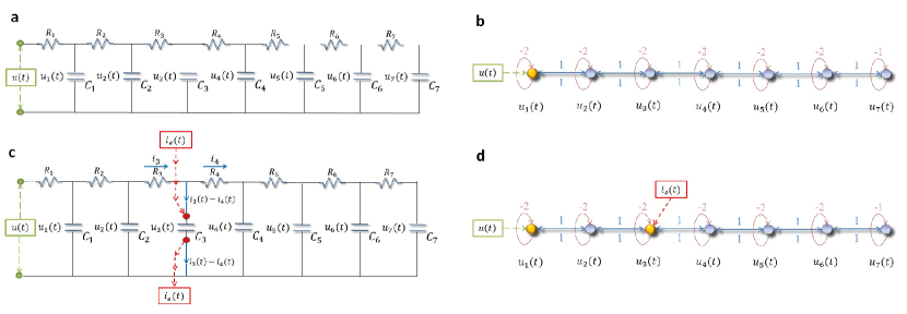
Figure 5: Cascade parallel R-C circuit and its corresponding network presentation. (a) A cascade parallel R-C circuit with $L=7$ resistors ($R_{1}$, $R_{2}$, $\ldots$, and $R_{L}$, each of resistance $1\Omega$) and $7$ capacitors ($C_{1}$, $C_{2}$, $\ldots$, and $C_{L}$, each of capacitance $1\mbox{F}$). External voltage input $u(t)$ is applied onto the left side of the circuit, and the voltage of capacitor $C_{i}$ is $u_{i}(t)(1\leq i\leq L)$. (b) Network representation of the circuit in (a) as a bidirectional 1D chain network of seven nodes, where the external voltage input $u(t)$ is injected into node $1$ (yellow driver node, the controller). The dynamical state of node $i$ is described by the voltage on its capacitor, $u_{i}(t)$. Links (blue) between nodes are bidirectional and have uniform weight $1$ in either direction. Each node has a self-link (red) of weight $-2$, except the ending node (node $7$) whose self-link has weight $-1$. (c) The circuit network in (b) with an extra external current input $i_{\text{e}}(t)$ into the capacitor $C_{3}$, where $i_{3}$ and $i_{4}$ denote the currents through resistors $R_{3}$ and $R_{4}$, respectively. In the absence of the extra current input, $i_{3}(t)-i_{4}(t)$ is the current through the branch of $C_{3}$. (d) The extra external current input $i_{\text{e}}(t)$ serves as a redundant control input injected into node $3$ of the network in (b). Now there are two driver nodes (yellow) in the network, nodes $1$ and $3$.

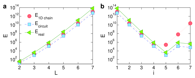
Figure 6: Control energy and optimization for 1D chain and cascade parallel R-C circuit. (a) Energy required for controlling a unidirectional chain (red) and the corresponding circuit (blue) as well as the dissipated energy of the circuit calculated from Eq. (6) versus the chain length $L$. (b) Control and dissipated energies in the presence of a redundant control signal to node $i$ ($i>1$), which breaks the chain into two subchains of lengths $i$ and $L-i$, respectively.

IV Control of real-world networks

IV.1 Control of an electrical circuit network

To further test the concept and framework of practical controllability, we consider a real one-dimensional cascade parallel R-C circuit network, as schematically illustrated in Fig. 5(a). The network can be represented by a bidirectional 1D chain with self-loops for all the nodes, as shown in Fig. 5(b). The network size can be enlarged, say by one unit, by attaching an additional branch of resistor and capacitor at the right end of the circuit. The state $u_{i}(t)$ of node $i$ at time $t$ is the voltage of capacitor $i$, and the input voltage $u(t)$ represents the control signal. The purpose of control is to drive the voltages of the capacitors from a set of values to another within time $t_{\text{f}}$ through the input voltage $u(t)$. The control energy can then be calculated by Eq. (4). The actual energy dissipated in the circuit during the control process is given by

$$E_{\text{real}}=\int_{0}^{t_{\text{f}}}U(t)\cdot I(t)dt,$$ (6)

where $U(t)\equiv u(t)$ and $I(t)$ are the input voltage and current at time $t$, and $E_{\text{real}}$ is in units of Joule. By making the circuit equivalent to a 1D chain network, we have three types of energy: the control energy of the actual circuit calculated from Eq. (4), the dissipated energy of the circuit from Eq. (6), and the control energy of the 1D equivalent network. Figure 6(a) shows that the control energy and the dissipated energy of the circuit do not differ substantially from the energy calculated from unidirectional 1D chain. Among the three types of energy, the energy cost associated with the control process, as calculated from Eq. (6), is maximal.

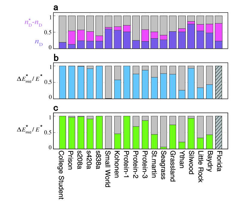
Figure 7: Augmented control inputs and energy optimization. (a) Densities of the original driver nodes $n_{\text{D}}$ (purple) and of the augmented controls $n^{\star}_{\text{D}}-n_{\text{D}}$ (pink). (b) Normalized energy reduction $\Delta E^{\star}_{\text{mid}}/E^{\star}=(E^{\star}-E^{\star}_{\text{mid}})/E^{\star}$ (blue) when an additional control signal is added to the middle of each LCC [strategy (I)]. (c) Normalized energy reduction $\Delta E^{\star}_{\text{end}}/E^{\star}=(E^{\star}-E^{\star}_{\text{end}})/E^{\star}$ (green) when an additional control signal is added to the end node of each LCC [strategy (II)]. For the blue bars (or green bars), the optimized control energy $E\star_{\text{mid}}$ (or $E\star_{\text{end}}$) is several orders of magnitude smaller than $E\star$. The bars with more gray portion the blue (or green) potions are for the networks with relatively low values of $E\star$ and $D_{\text{C}}$ (see Table A2 in Appendix F), for which energy optimization is not necessary. The bar corresponding to “Florida” (the most right) is striped due to the fact that this network is not controllable (i.e., with divergent energy) even if $M\star$ augmented control inputs are added.

IV.2 Strategies to balance control energy and extra inputs

Our finding of the LCC structure associated with the control and the exponential growth of energy with the length of LCCs suggest a method to reduce the energy significantly. Since the key topological structure that determines the control energy is LCCs, one possible approach is to reduce the length of all the LCCs embedded in a network by making structural perturbations to the network. This, however, will inevitably modify the network structure, which may not always be practically viable. Is it possible to reduce the control energy without having to change the network structure? One intuitive method is to apply additional controllers beyond those calculated from the structural-controllability theory, which we name as redundant controllers. A straightforward solution is to add some redundant control signals along the LCCs. To gain insights, we consider a unidirectional 1D chain and add a redundant control input at the $i$th node. As shown in Fig. 6(b), the magnitude of control energy is reduced dramatically. The optimal location to place the extra control should be near the middle of the chain so as to minimize the length of LCCs using a minimal number of redundant control signals. As can be seen from Fig. 6(b), this simple strategy of adding one redundant control signal can reduce the required energy by nearly seven orders of magnitude! More specifically, the redundant control signal to node $i$ breaks a chain of length $L$ into two shorter subchains: one of length $i-1$ and another of length $L-i+1$. Roughly, the control energy is the sum of energies required to control the two shorter components, which is dominated by energy associated with the longer component owing to the exponential dependence of the energy on the chain length. By choosing $i$ around $L/2$, the length of the longer part is minimized. For the circuit network in Fig. 5, the redundant control input can be realized by inducing external current input into a capacitor. As shown in Fig. 5(b), a reduction in energy of nearly $10$ orders of magnitude is achieved. Applying a single redundant control input can thus be an extremely efficient strategy to reduce the required control energy for the one-dimensional chain network.

Due to the fact that there can be multiple LCCs converge at the same end node, applying a control signal to each of the $m$ nodes that all LCCs converge into is another strategy that reduces the total number of redundant controls, while also significantly shrinks the control energy. (Detailed demonstrations of the enhancement strategies for physical or modeled networks and an implementation example on a circuit system are presented in Appendix G.)

IV.3 Control of real-world networks

Can real-world complex networks be actually controlled? In Ref. Liu et al. (2011), the structural controllability of a large number of real-world networks were investigated, with the conclusion that optimal control of most of the networks can be achieved with only a few control signals. We investigate control energies of the same set of real-world networks (see Table A1 in Appendix F for network details) and find that, when optimal control is applied according to maximum matching, most of the networks require realistically high energies. In fact, $15$ out of the $18$ networks are practically uncontrollable. The main reason lies in the large LCCs of most of these networks. Another factor is that there are subgraphs that are not connected with each other and/or a large number of topological motifs such as loops, self-loops, or bidirectional edges. More strikingly, even with unlimited energy supply, the number of driver nodes as determined by the maximum matching algorithm from the structural controllability theory is generally insufficient to fully control the whole system, where there exists a number $M^{\star}$ of nodes that never converge to their target states. These observations lead to the speculation that, in order to fully control a realistic network, more driver nodes are needed than those identified by the structural controllability theory. That is, more independent control signals are needed than those determined by maximum matching to drive all nodes in the network to their target states. The $M^{\star}$ uncontrollable nodes are thus the required augmented set of driver nodes, each with an external control input. In total, $N_{D}^{\star}=N_{D}+M^{\star}$ driver nodes need to be deployed to gain full control of the system [see Fig. 7(a) for $n_{D}$ and $n_{D}^{\star}=N_{D}^{\star}/N$ for the $18$ real-world networks]. Applying control signals to the nodes as determined by maximum matching and to the augmented driver nodes, we find that $17$ out $18$ real-world networks become practically controllable (see Table A2 in Appendix F).

We also test the enhancement strategies using the $18$ real-world networks, with the result that their practical controllability can be markedly enhanced (especially for those with large control diameters), as shown Figs. 7(b) and (c). We see that, for each of the real-world networks with unrealistically large energy requirement (see Table A2 in Appendix F), the optimized control energy $E^{\star}_{\text{mid}}$ (or $E^{\star}_{\text{end}}$) is several orders of magnitude smaller than the value of the original energy $E^{\star}$ (the control energy with $M^{\star}$ augmented driver nodes but without any redundant control input). This indicates the effectiveness of our optimization strategies. (In fact, strategy (I) works better than (II) in most cases.) For the networks with small control diameters, even without applying any enhancement strategy the control energies required are already much smaller than those for the other networks. For these networks energy optimization is practically unnecessary (see also Table A2 in Appendix F).

We also find that increasing the control time $t_{\text{f}}$ can reduce the control energy so as to enhance the network’s practical controllability.

V Conclusions and Discussions

As stated in Ref. Liu et al. (2011), the ultimate proof that one understands a complex network completely lies in one’s ability to control it. We discover a paradox arising from controlling complex networks with respect to control energy and the number of external input signals. To resolve the paradox, we focus on the situation where the structural-controllability theory yields a minimum number of external input signals required for full control of the network, and determine whether in these situations the control energy is affordable so as to realize actual control. Our systematic computations and analysis reveal a rather unexpected phenomenon: due to the singular nature of the control Gramian matrix, in the parameter regimes where optimal structural controllability is achieved in the sense that the number of driver nodes is minimized, energy consumption can be unbearably large. To obtain a more systematic understanding, we identify the fundamental structures in a network under the action of control signals, the longest control chains (LCCs), and argue that they essentially determine the control energy. We articulate and validate that the required energy increases exponentially with the length of the LCCs. In situations where the required number of controllers is few as determined by the structural controllability theory, the length of LCCs tends to be long, leading to practically divergent control energy. Another finding is that, for minimum input signals, the required energy exhibits a robust algebraic scaling behavior, which can be explained by analyzable models constructed based on interacting LCCs. The discovery of the LCCs associated with controlling complex networks leads naturally to a simple method to resolve the paradox: increasing the number of controllers by placing extra control signals (beyond the number determined by the structural-controllability theory) along the LCCs. Indeed, test of a large number of real-world networks shows that, while they are structurally controllable Liu et al. (2011), most of them exhibit enormous energy consumption. They can actually be controlled by placing more drivers than determined by the structural-controllability theory at proper locations along the LCCs.

Our work indicates that the difficulty of achieving actual control of complex networks associated with even linear dynamics is beyond the current knowledge in the field of network control. Although the controllability theory offers a theoretically justified framework to guide us to apply external inputs on a minimum set of driver nodes, when we implement control to steer a system to a desired state, the energy consumption is likely to be too large to be affordable. This finding suggests that, to achieve control of a complex networked system, the existing controllability framework merely offers a necessary rather than a practically feasible condition to assure actual control. We thus demand a more comprehensive and practically useful theoretical framework for addressing the extremely important issue of controlling complex networks. However, it is difficult to develop such a framework at the present and we do not even know if a mathematically justified theory is available based on the current knowledge. Another issue is that for general networked nonlinear systems, we continue to lack the necessary condition based on the present controllability framework, as well as an understanding of required control energy. So far, we still know too little about controlling complex networked systems, and further effort is needed to address this challenging but greatly important problem shared by a wide range of fields.

Appendix A: Analytical calculation of the in- and out-degree distributions

The in- and out-degree distributions of a directed complex network under connection bias probability $\lambda\equiv P_{\text{b}}$ can be obtained analytically.

Defining $k_{\text{S}}$ and $k_{\text{L}}$ to be the numbers of nodes in the neighborhood of a node with degree $k$, whose degrees are smaller or larger than than $k$, respectively, we have

$$k_{\text{S}}=k\sum_{k^{\prime}=k_{\text{min}}}^{k}P(k^{\prime}|k)=\frac{k}{\langle k\rangle}\sum_{k_{\text{min}}}^{k}k^{\prime}P(k)=\frac{k}{\langle k\rangle}\int_{k_{\text{min}}}^{k}k^{\prime}\cdot Ck^{\prime-\gamma}\,\mathrm{d}k^{\prime}=\frac{Ck}{\langle k\rangle}\int_{k_{\text{min}}}^{k}k^{\prime 1-\gamma}\,\mathrm{d}k^{\prime},$$ (A1)

and

$$k_{\text{L}}=k\sum_{k^{\prime}=k}^{k_{\text{max}}}P(k^{\prime}|k)=\frac{Ck}{\langle k\rangle}\int_{k}^{k_{\text{max}}}k^{\prime 1-\gamma}\,\mathrm{d}k^{\prime}\stackrel{{\scriptstyle\gamma>2}}{{=}}\frac{Ck^{3-\gamma}}{\langle k\rangle(\gamma-2)}=Ak^{3-\gamma},$$ (A2)

where

$$A=\frac{C}{\langle k\rangle(\gamma-2)}.$$ (A3)

Therefore,

$$k_{\text{S}}=k-k_{\text{L}}.$$ (A4)

We then have

$$k_{\text{out}}=\lambda k_{\text{S}}+(1-\lambda)k_{\text{L}}=\lambda(k-k_{\text{L}})+(1-\lambda)k_{\text{L}}=(1-2\lambda)k_{\text{L}}+\lambda k=(1-2\lambda)Ak^{3-\gamma}+\lambda k,$$ (A5)

and

$$k_{\text{in}}=(1-\lambda)k_{\text{S}}+\lambda k_{\text{L}}=(1-\lambda)k+(2\lambda-1)Ak^{3-\gamma}.$$

The quantities $P(k_{\text{out}})$ and $P(k_{\text{in}})$ can be derived from

$$P(k_{\text{out}})\,\mathrm{d}k_{\text{out}}=P(k)\,\mathrm{d}k\ \ \mbox{and}\ \ P(k_{\text{in}})\,\mathrm{d}k_{\text{in}}=P(k)\,\mathrm{d}k,$$ (A6)

which yield

$$P(k_{\text{out}})=P(k)\frac{\,\mathrm{d}k}{\,\mathrm{d}k_{\text{out}}}\ \ \mbox{and}\ \ P(k_{\text{in}})=P(k)\frac{\,\mathrm{d}k}{\,\mathrm{d}k_{\text{in}}}.$$ (A7)

Setting $k=f_{1}^{-1}(k_{\text{out}})$ and $k=f_{2}^{-1}(k_{\text{in}})$, we can obtain the distributions.

Using

$$k_{\text{out}}=f_{1}(k)\ \ \mbox{and}\ \ k_{\text{in}}=f_{2}(k),$$

we obtain

$$P(k_{\text{out}})=P(k)\frac{1}{\frac{\,\mathrm{d}k_{\text{out}}}{\,\mathrm{d}k}}=P(f_{1}^{-1}(k_{\text{out}}))\frac{1}{f_{1}^{\prime}(f_{1}^{-1}(k_{\text{out}}))},$$ (A8)

and

$$P(k_{\text{in}})=P(f_{2}^{-1}(k_{\text{in}}))\frac{1}{f_{2}^{\prime}(f_{2}^{-1}(k_{\text{in}}))}.$$ (A9)

In general, it is difficult to obtain an explicit expression. However, for some specific values of $\lambda$ or $\gamma$, analytical results are available.

Case I: $\lambda=0.5$.

In this case, we have

$$k_{\text{out}}=k_{\text{in}}=\frac{k}{2},$$ (A10)

and

$$k=2k_{\text{out}}=2k_{\text{in}}.$$ (A11)

Thus

$$P(k_{\text{out}})=2P(2k_{\text{out}})=2C(2k_{\text{out}})^{-\gamma}=2^{1-\gamma}Ck_{\text{out}}^{-\gamma}.$$

Akin to $P(k_{\text{out}})$, we have

$$P(k_{\text{in}})=P(k_{\text{out}})=2^{1-\gamma}Ck_{\text{in}}^{-\gamma}.$$

Case II: $\lambda=0$.

$$k_{\text{out}}=Ak^{3-\gamma}\Rightarrow k=\frac{k_{\text{out}}}{A}^{\frac{1}{3-\gamma}}.$$ (A12)

We then have

$$P(k_{\text{out}})=C(\frac{k_{\text{out}}}{A})^{\frac{1}{3-\gamma}(-\gamma)}\frac{\,\mathrm{d}k}{\,\mathrm{d}k_{\text{out}}}=C(\frac{k_{\text{out}}}{A})^{\frac{\gamma}{\gamma-3}}\frac{1}{3-\gamma}\bigg{(}\frac{k_{\text{out}}}{A}\bigg{)}^{\frac{1}{3-\gamma}-1}\frac{1}{A}=\frac{C}{3-\gamma}A^{\frac{1}{3-\gamma}}k_{\text{out}}^{\frac{2}{\gamma-3}}.$$

Case III: $\lambda=1$.

$$k_{\text{in}}=Ak^{3-\gamma}\Rightarrow k=\frac{k_{\text{in}}}{A}^{\frac{1}{3-\gamma}},$$ (A13)

which yields

$$P(k_{\text{in}})=P(k_{\text{out}})=\frac{C}{3-\gamma}A^{\frac{1}{3-\gamma}}k_{\text{in}}^{\frac{2}{\gamma-3}}.$$ (A14)

Case IV: $\gamma=3$. For example, for BA model, we have

$$k_{\text{out}}=(1-2\lambda)A+\lambda k,$$ (A15)

and

$$k=\frac{k_{\text{out}}+(2\lambda-1)A}{\lambda}.$$ (A16)

$$P(k_{\text{out}})=C\bigg{(}\frac{k_{\text{out}}+(2\lambda-1)A}{\lambda}\bigg{)}^{-\gamma}\frac{1}{\lambda}=C\lambda^{\gamma-1}\bigg{[}k_{\text{out}}+(2\lambda-1)\frac{C}{\langle k\rangle}\bigg{]}^{-\gamma}=C\lambda^{\gamma-1}\bigg{[}k_{\text{out}}+(2\lambda-1)k_{\text{min}}\bigg{]}^{-\gamma}.$$

Similarly, we have

$$k_{\text{in}}=(2\lambda-1)A+(1-\lambda)k,$$ (A17)

and

$$k=\frac{k_{\text{in}}+(1-2\lambda)A}{1-\lambda},$$ (A18)

so

$$P(k_{\text{in}})=C\bigg{[}\frac{k_{\text{in}}+(1-2\lambda)A}{1-\lambda}\bigg{]}^{-\gamma}\frac{1}{1-\lambda}=C(1-\lambda)^{\gamma-1}[k_{\text{in}}+(1-2\lambda)k_{\text{min}}]^{-\gamma}.$$ (A19)

Appendix B: Additional numerical results

B1: Condition number and control error.

The correlation between the condition number $C_{W}$ and the control error $e_{X}$ is shown in Fig. A1. We observe that, within a certain range of $C_{W}$, an approximate scaling relation exists between $C_{W}$ and $e_{X}$, shown in panels (a), (c), (e), and (g). However, the scaling disappears outside the shown $C_{W}$ range. The reason is that, outside the $C_{W}$ range, the Gramian matrix $W$ is ill conditioned, leading to considerable errors when computing the matrix inverse. In principle, the scaling regime can be extended with improved computational precision, but not indefinitely.

B2: More on structural and practical controllability measures.

Figure A2 shows the measure of the structural controllability, $n_{\text{D}}$, and the measure of the practical controllability, $P(\bar{C_{W}})$, versus $P_{\text{b}}$ for ER random and BA scale-free networks of size $N=200$. We see that the structural and practical controllability cannot be simultaneously optimized irrespective of the network size.

B3: More on control energy power law distribution.

Figure A3 shows the robustness of the control energy power-law distribution against varying network size for both random [(a)] and scale-free [(b)] topology.

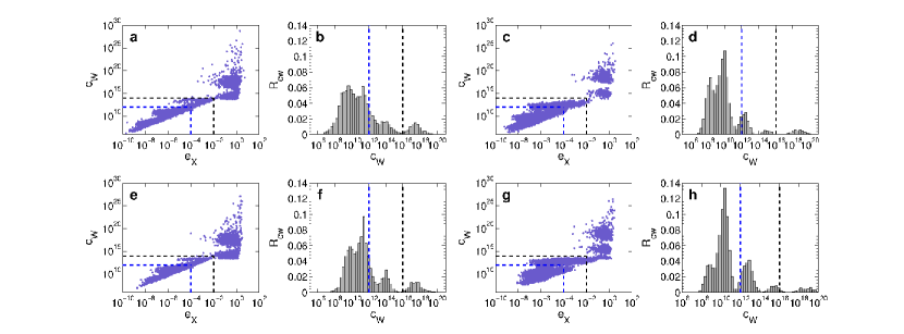
Figure A1: Condition number $C_{W}$ versus control error $e_{X}$ for random and scale-free networks. Network size is $N=100$ for (a-d) and $200$ for (e-h), average degree is $\langle{k}\rangle=6$ for ER random networks [(a),(b),(e), and (f)] and $8$ for BA scale-free networks [(c), (d), (g), and (h)]. Directional link probability between any pair of nodes is $P_{\text{b}}=0.1$. Panels (a),(c),(e), and (g) show the scaling relation between the condition number $C_{W}$ and control error $e_{X}$. Panels (b), (d), (f), and (h) show the fraction $R_{CW}$ of the networks with a certain $C_{W}$ number. The scaling relation holds within some $C_{W}$-$e_{X}$ region with boundaries specified as the black dashed lines. The $e_{X}$ values are not physically meaningful outside the boundaries that are defined according to the precision limit of computation. The thresholds of $C_{W}$ and $e_{X}$ used in the computations are $10^{12}$ and $10^{-4}$, respectively, which are indicated as the blue dashed lines. The threshold values are chosen to lie within the physical boundaries so that the calculations for all $C_{W}$ values are meaningful.

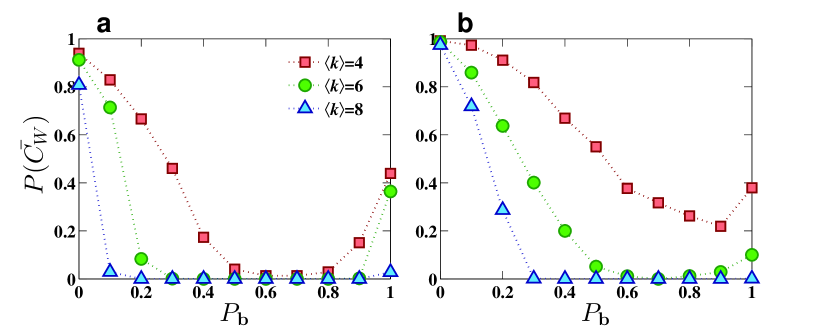
Figure A2: Practical controllability measures for directed networks. Measure of the practical controllability, $P(\bar{C}_{W})$, for (a) ER random networks and (b) BA scale-free networks of size $N=200$.

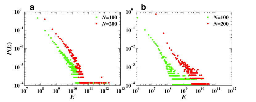
Figure A3: Distributions of control energy for practically controllable networks under different network sizes. Panels (a) and (b) are for random networks with $\langle k\rangle=6$ and scale-free networks with $\langle k\rangle=8$, respectively, for two values of the network size ($N=100$ and $N=200$), where we set $\bar{C}_{W}=10^{12}$ and $t_{\text{f}}=1$. In all cases, we observe an algebraic (power-law) scaling behavior.

Appendix C: Control Energy of One-Dimensional String

As shown in Fig. A4, the energy required to control a unidirectional 1D string nearly overlaps with that of a bidirectional one with identical weights. In fact, if the chains are not too long, the relative difference in the energy between the two case are within the same order of magnitude. Here we provide an analytical calculation of the control energy for a bidirectional 1D chain network.

The energy $E$ is given by

$$E(t_{\text{f}})=\mathbf{x}_{0}^{T}\cdot H^{-1}\cdot\mathbf{x}_{0},$$ (A20)

where $H\equiv e^{-At_{\text{f}}}\cdot W\cdot e^{-A^{T}t_{\text{f}}}$, $\mathbf{x}_{0}$ is the initial state of the network, and $W$ is the Gramian matrix. Since $H$ is positive definite and symmetric, its inverse $H^{-1}$ can be decomposed in terms of its eigenvectors as $H^{-1}=Q\Lambda Q^{T}$, where $Q=[q_{1},q_{2},\dots,q_{N}]$ is composed of the orthonormal eigenvectors that satisfy $QQ^{T}=Q^{T}Q=I$, and $\Lambda=\mbox{diag}\{\lambda_{1},\lambda_{2},\dots,\lambda_{N}\}$ is the diagonal eigenvalue matrix of $H^{-1}$ in descending order. Numerically, we find that $\lambda_{1}$ is typically much larger than other eigenvalues. We thus have

$$E(t_{\text{f}})=\mathbf{x}_{0}^{T}Q\Lambda Q^{T}\mathbf{x}_{0}=\sum_{i=1}^{n}\lambda_{i}(q_{i}^{T}\mathbf{x}_{0})^{2}\approx\lambda_{1}(q_{1}^{T}\mathbf{x}_{0})^{2}.$$ (A21)

Since $\mathbf{x}_{0}$ can be chosen arbitrarily, we set $\mathbf{x}_{0}=[1,0,\dots,0]^{T}$, so Eq. (A21) becomes

$$E(t_{\text{f}})\approx\lambda_{1}(q_{1}^{T}q_{1})=\lambda_{1}.$$ (A22)

For an undirected network, the adjacency matrix $A$ is positive definite and symmetric. We can decompose $A$ into the form $A=VSV^{T}$, where the columns of $V$ constitute the orthonormal eigenvectors of $A$ and $S=\mbox{diag}\{s_{1},s_{2},\dots,s_{N}\}$ is the diagonal eigenvalue matrix of $A$ in descending order. We thus have $H=e^{-At_{\text{f}}}We^{-A^{T}t_{\text{f}}}=Ve^{-St_{\text{f}}}V^{T}WVe^{-St_{\text{f}}}V^{T}$. Let

$$\Lambda_{H}=\mbox{diag}\{\lambda_{H_{1}},\lambda_{H_{2}},\dots,\lambda_{H_{N}}\}=\mbox{diag}\{1/\lambda_{N},1/\lambda_{N-1},\dots,1/\lambda_{1}\}$$

be the eigenvalue matrix of $H$ in descending order. The energy can thus be expressed as

$$E(t_{\text{f}})\approx\lambda_{1}(q_{1}^{T}\mathbf{x}_{0})^{2}=\lambda_{H_{N}}^{-1}(q_{1}^{T}\mathbf{x}_{0})^{2}.$$

Letting $\Lambda_{W}=\mbox{diag}\{\lambda_{W_{1}},\lambda_{W_{2}},\dots,\lambda_{W_{N}}\}$ be the eigenvalue matrix of $W$ in descending order. We can approximate the eigenvalue of $H$ by $W$, which has been numerically validated: $\Lambda_{H}\approx\Lambda_{W}$. We thus have

$$\varepsilon\approx\lambda_{1}(q_{1}^{T}\mathbf{x}_{0})^{2}=\lambda_{H_{N}}^{-1}(q_{1}^{T}\mathbf{x}_{0})^{2}\approx\lambda_{W_{N}}^{-1}(q_{1}^{T}\mathbf{x}_{0})^{2}.$$ (A23)

Since orthonormal transform does not alter the eigenvalues of a given matrix, we have $\Lambda_{H}=e^{-St_{\text{f}}}\Lambda_{W}e^{-St_{\text{f}}}$.

For an undirected chain, the adjacency matrix is

$$A=\begin{bmatrix}0&1&&&\\ 1&0&\ddots&&\\ &1&\ddots&1&\\ &&\ddots&0&1\\ &&&1&0\end{bmatrix}_{N\times N},$$

control matrix is $B=[1,0,\dots,0]^{T}$, and eigenvalues and eigenvectors of $A$ are

$$s_{i}=2\cos\left(\frac{\pi}{N+1}i\right),\quad i=1,\dots,N,$$ (A24)

$$V_{j}^{(i)}=\sqrt{\frac{2}{N+1}}\sin\left(\frac{\pi}{N+1}ij\right),\quad i,j=1,\dots,N.$$ (A25)

Recall that $H=Ve^{-St_{\text{f}}}(\int_{0}^{t_{\text{f}}}e^{St}V^{T}BB^{T}Ve^{St}\,\mathrm{d}t)e^{-St_{\text{f}}}V^{T}$. Substituting this in Eqs. (A24) and (A25), after some algebraic manipulation, we obtain

$$H=\frac{1}{N+1}VWPWV^{T},$$ (A26)

where

$$W=\begin{bmatrix}\sin(\theta)&&&\\ &\sin(2\theta)&&\\ &&\ddots&\\ &&&\sin(N\theta)\end{bmatrix}_{N\times N}$$

and

$$P_{jk}=\int_{0}^{2t_{\text{f}}}\,e^{-[\cos(j\theta)+\cos(k\theta)]t}\,\mathrm{d}t$$

with $\theta=\pi/(N+1)$, $j,k=1,\cdots,N$.

As a result, we have $S=\mbox{diag}\{2cos(\frac{\pi}{N+1}),2cos(\frac{2\pi}{N+1}),...,2cos(\frac{N\pi}{N+1})\}$. The minimum eigenvalue of $H$ is given by

$$\lambda_{H_{N}}=e^{-2cos(\frac{N\pi}{N+1})t_{\text{f}}}\lambda_{W_{N}}e^{-2cos(\frac{N\pi}{N+1})t_{\text{f}}}=e^{-4cos(\frac{N\pi}{N+1})t_{\text{f}}}\lambda_{W_{N}}=1/\lambda_{1}.$$ (A27)

The Rayleigh-Ritz theorem can be used to bound $P$ as:

$$\lambda_{P_{N}}\leq\frac{y^{T}Py}{y^{T}y}\leq\lambda_{P_{1}},$$ (A28)

where $y=[y_{1},y_{2},\dots,y_{N}]^{T}$ is an arbitrary nonzero column vector, $\lambda_{P_{N}}$ and $\lambda_{P_{1}}$ are the maximal and minimal eigenvalues of $P$, respectively. Letting $T=2t_{\text{f}}$, we have

$$y^{T}Py =(y_{1}\cdots y_{N})\left[\int_{0}^{T}\,e^{-[\cos(j\theta)+\cos(k\theta)]\tau}\,\mathrm{d}\tau\right]_{N\times N}\begin{pmatrix}y_{1}\\ \vdots\\ y_{N}\end{pmatrix}$$

$$=\sum_{j,k=1}^{N}\,y_{j}y_{k}\int_{0}^{T}\,e^{-[\cos(j\theta)+\cos(k\theta)]\tau}\,\mathrm{d}\tau$$

$$=\sum_{j,k=1}^{N}\,\langle y_{j}e^{-[\cos(j\theta)t]},y_{k}e^{-[\cos(k\theta)t]}\rangle$$

$$=\langle\sum_{j=1}^{N}\,y_{j}e^{-[\cos(j\theta)]t},\sum_{j=1}^{N}\,y_{j}e^{-[\cos(j\theta)]t}\rangle,$$ (A29)

with $\langle f,g\rangle\equiv\int_{0}^{T}\,fg\,\mathrm{d}\tau$.

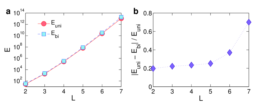
Figure A4: Comparison between energies required to control a unidirectional and a bidirectional 1D chains: (a) energies required to control a unidirectional chain $E_{\text{uni}}$ (red) and a bidirectional one $E_{\text{{bi}}}$ (blue) versus chain length $L$, and (b) the relative energy difference $|E_{\text{{uni}}}-E_{\text{bi}}|/E_{\text{{uni}}}$ versus chain length $L$.

Letting $b_{j}=e^{-\cos(j\theta)}$ and performing a Taylor expansion of $b_{j}^{t}$ around $t=0$, we obtain

$$b_{j}^{t}=\sum_{k=0}^{N-1}\,[-\cos(j\theta)]^{k}\frac{t^{k}}{k!}+[-\cos(j\theta)]^{N}\frac{t_{j}^{N}}{N!}$$ (A30)

with $t_{j}\in[0,T]$. Now letting

$$q_{j}(t)=\sum_{k=0}^{N-1}\,[-\cos(j\theta)]^{k}\frac{t^{k}}{k!},$$

we have $b_{j}^{t}=q_{j}(t)+[-\cos(j\theta)]^{N}\cdot(t_{j}^{N}/N!)$. Consequently, the numerator in the Rayleigh quotient can be expressed as

$$y^{T}Py= \langle\sum_{j=1}^{N}\,y_{j}b_{j}^{t},\sum_{j=1}^{N}\,y_{j}b_{j}^{t}\rangle$$

$$= \langle\sum_{j=1}^{N}\,\left(y_{j}q_{j}(t)+y_{j}[-\cos(j\theta)]^{N}\frac{t_{j}^{N}}{N!}\right),\sum_{j=1}^{N}\,\left(y_{j}q_{j}(t)+y_{j}[-\cos(j\theta)]^{N}\frac{t_{j}^{N}}{N!}\right)\rangle$$

$$= \langle\sum_{j=1}^{N}\,y_{j}q_{j}(t),\,\sum_{j=1}^{N}\,y_{j}q_{j}(t)\rangle+2\langle\sum_{j=1}^{N}\,\,y_{j}q_{j}(t),\sum_{j=1}^{N}\,y_{j}[-\cos(j\theta)]^{N}\frac{t_{j}^{N}}{N!}\rangle$$

$$+\langle\sum_{j=1}^{N}\,y_{j}[-\cos(j\theta)]^{N}\frac{t_{j}^{N}}{N!},\,\sum_{j=1}^{N}\,y_{j}[-\cos(j\theta)]^{N}\frac{t_{j}^{N}}{N!}\rangle$$

$$\leq \underbrace{\langle\sum_{j=1}^{N}\,\,y_{j}q_{j}(t),\sum_{j=1}^{N}\,y_{j}q_{j}(t)\rangle}_{\text{Denote as }K_{1}}+\underbrace{2\frac{T^{N}}{N!}\sum_{k=1}^{N}\,|y_{k}|\left(\left|\langle\sum_{j=1}^{N}\,y_{j}q_{j}(t),1\rangle\right|\right)}_{\text{Denote as }K_{2}}$$

$$+\underbrace{\left(\frac{T^{N}}{N!}\right)^{2}\sum_{j,k=1}^{N}\,|y_{j}y_{k}|T}_{\text{Denote as}K_{3}}.$$ (A31)

Since $y=[y_{1},y_{2},\dots,y_{N}]^{T}$ is an arbitrary nonzero column vector, for each $N$ and $T$, we can choose $y=y_{m}$ insofar as $K_{1}$ and $K_{2}$ are relatively small compared with $K_{3}$. We can normalize $y_{m}^{T}y$ to arrive at

$$\lambda_{P_{N}}\leq\frac{y_{m}^{T}Py_{m}}{y_{m}^{T}y_{m}}=\left(\frac{T^{N}}{N!}\right)^{2}\sum_{j,k=1}^{N}\,|y_{m_{j}}y_{m_{k}}|T\thicksim O\left(\frac{T^{2N}}{(N!)^{2}}\right),$$ (A32)

where $\lambda_{P_{N}}$ is the smallest eigenvalue of $P$. Recall that $P$ is symmetric and positive definite, using Cholesky decompostion we can obtain its factorization Strang (1976) as $P=LL^{T}$, where $L$ is the lower triangular matrix with its diagonal filled with square roots of eigenvalues of $P$. Therefore, Eq. (A26) can be written as $H=\frac{1}{N+1}VWLL^{T}WV^{T}$. Since orthonormal transform does not change the eigenvalues of a matrix, $H$ has the same eigenvalues as $R=\frac{1}{N+1}WLL^{T}W=\frac{1}{N+1}WL(WL)^{T}$. Suppose $\Lambda_{P}=\mbox{diag}\{\lambda_{P_{1}},\lambda_{P_{2}},\dots,\lambda_{P_{N}}\}$ is the diagonal eigenvalue matrix of $P$ in descending order. The $j$th eigenvalue of $R$ satisfies

$$\lambda_{R_{j}}=\frac{1}{N+1}\lambda_{P_{j}}(\sin k\theta)^{2}\leq\frac{1}{N+1}\lambda_{P_{j}},$$

where $j$ and $k$ run from $1$ to $n$. The control energy $E(t_{\text{f}})$ can then be approximated as

$$E(t_{\text{f}})\approx\lambda_{H_{N}}^{-1}\thicksim O\left((N+1)\frac{(N!)^{2}}{t_{\text{f}}^{2N}}\right).$$ (A33)

Appendix D: Correlation between network control energy and smallest eigenvalue of $H$-matrix

Strong correlation between the average network control energy, $\langle E\rangle$, and the smallest eigenvalue of the $H$-matrix, $\lambda_{H_{N}}^{-1}$, for ER random and BA scale-free networks can be observed in Fig. A5, indicating that the network control energy is essentially determined by the smallest eigenvalue of its $H$-matrix.

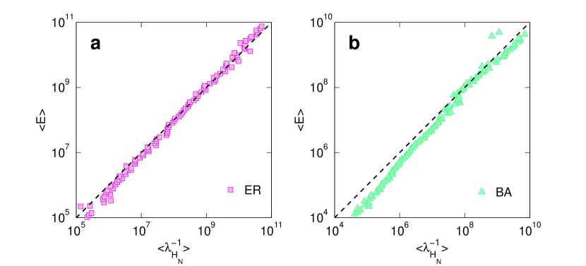
Figure A5: Correlation between network control energy and the smallest eigenvalue of $H$-matrix. Network size is $N=100$, directional link probability between any pair of nodes is $P_{\text{b}}=0.1$, and average degree is (a) $\langle k\rangle=6$ for ER random networks and (b) $\langle k\rangle=8$ for BA sale-free networks.

Appendix E: LCC-skeleton and double-chain interaction models

E1: LCC-skeleton model.

Referring to Fig. 4 in the main text, we assume that the control chains are independent of each other so that $E_{2}$ is negligible as compared with $E_{1}$. Each control chain is effectively a 1D string. Due to the exponential increase in energy via chain length increment, $E_{1}$ can be regarded as the sum of control energies associated with the set of unidirectional 1D strings, to which the contribution of the LCC dominates. The required energy to control the full network can thus be approximated as that required to control all LCCs,

$$E=E_{1}+E_{2}\approx E_{1}\approx m\cdot E_{L}\approx m\cdot\lambda_{H_{L}}^{-1},$$ (A34)

where $E_{L}$ denotes the energy required to control an LCC, $\lambda_{H_{L}}$ is the smallest eigenvalue of the LCC’s $H$ matrix $H_{L}$, and $m$ denotes the degeneracy (multiplicity) of the LCC, as shown in Fig. 4(b) in the main text. Results presented in Fig. 3(b) of the main text demonstrate a positive correlation between $E$ and $m\cdot E_{L}$, reinforcing the idea the independent LCCs are the key topological structure dictating the energy required to control the whole network. In particular, if a network contains long LCCs (as can be determined straightforwardly by maximum matching from the structural controllability theory Liu et al. (2011)), there is high likelihood that it cannot be practically controlled as practically the required energy would diverge.

Reasoning from an alternative standpoint, an arbitrary combination of $D_{\text{C}}$ and $m$ effectively represents a network, as shown in Fig. 4(b) in the main text, and the entire network ensemble can be represented by the ensemble of all possible combinations of LCCs. In the LCC ensemble, the quantities $D_{\text{C}}$ and $m$ emerge according to their probability density functions, $P_{D_{\text{C}}}(D_{\text{C}})$ and $P_{m}(m)$, respectively, and the appearance of an arbitrary pair of $D_{\text{C}}$ and $m$ is determined by their joint probability density function $P(D_{\text{C}},m)$. Consequently, the distribution of the energy required to control the original network can be characterized accurately by the distribution of the energy required to control the LCC skeleton in the corresponding ensemble.

Figure A6(a) shows the distribution of the control diameter $D_{\text{C}}$, essentially the length distribution of LCCs. The probability density function decays approximately exponentially with $D_{\text{C}}$, so we write

$$P_{D_{\text{C}}}(D_{\text{C}})=a\cdot e^{-b\cdot D_{\text{C}}},$$ (A35)

where $a$ and $b$ are positive constants. Using the relationship between $E_{L}$ and $D_{\text{C}}$ [e.g., Fig. 3(a) in the main text], we have

$$E_{L}\approx A\cdot e^{B\cdot D_{\text{C}}}\Rightarrow D_{\text{C}}\approx\frac{1}{B}\ln{\frac{E_{L}}{A}},$$ (A36)

where $A$ and $B$ are positive constants. The probability density function of $E_{L}$ can then obtained as

$$P_{L}(E_{L})=P_{D_{\text{C}}}(\frac{1}{B}\ln\frac{E_{L}}{A})\cdot|\frac{\,\mathrm{d}(\frac{1}{B}\ln\frac{E_{L}}{A})}{\,\mathrm{d}E_{L}}|\approx\frac{a}{B}A^{\frac{b}{B}}\cdot E_{L}^{-(1+\frac{b}{B})}.$$ (A37)

In the ER random network ensemble, the probability density of LCC degeneracy $m$ for networks with $D_{\text{C}}>2$ also exhibits an exponential decay, as shown in Fig. A6(b):

$$P_{m}(m)=c\cdot e^{-g\cdot m},$$ (A38)

where $c$ and $d$ are positive constants.

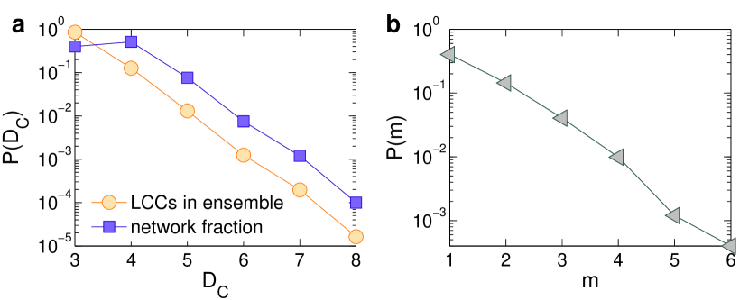
Figure A6: Probability distribution of control diameter and its degeneracy. (a) Distribution of $D_{\text{C}}$ (blue) and the probability that an LCC of length $D_{\text{C}}$ appears in the random network ensemble versus $D_{\text{C}}$. (b) Probability distribution of LCC-degeneracy $m$ for networks with $D_{\text{C}}>2$.

Since the control energy depends monotonously on the control diameter $D_{\text{C}}$, the energy dependence on $m$ can be revealed by examining the correlation between $D_{\text{C}}$ and $m$, which can in general be either positive or negative. From Eq. (A38), we see that $P_{m}(m)$ increases exponentially with $m$, implying a positive correlation:

$$D_{\text{C}}=s_{1}+s_{2}\cdot m,$$ (A39)

where $s_{1}$ and $s_{2}$ are positive constants. This form of relation ensures that $P_{m}(m)$ has the form in Eq. (A38). Positive correlation, however, means that the number of LCCs increases with its length, which is unphysical for random networks. These arguments suggest that a contradiction can arise if we assume either positive or negative correlation between $D_{\text{C}}$ and $m$. A natural resolution is that these two quantities are independent of each other. Since $E_{L}$, the energy required to control a chain of length $L$, is determined mainly by the control diameter $D_{\text{C}}$, $E_{L}$ and $m$ can be assumed to be independent of each other so that their joint probability density function can be expressed as $P(E_{L},m)\approx P_{L}(E_{L})\cdot P_{m}(m)$.

Having obtained $P_{L}(E_{L})$ and $P_{m}(m)$, we can calculate the cumulative probability distribution function of the estimated control energy $E=m\cdot E_{L}$ required to control the original network. We have

$$F_{E}(E)=P(m\cdot E_{L}<E)=\int_{0}^{\infty}[\int_{0}^{\frac{E}{E_{L}}}P(E_{L},m)\cdot\,\mathrm{d}m]\,\mathrm{d}E_{L}$$ (A40)

$$=\int_{0}^{\infty}[\int_{0}^{\frac{E}{E_{L}}}P_{L}(E_{L})\cdot P_{m}(m)\cdot\,\mathrm{d}m]\,\mathrm{d}E_{L}\approx\frac{caA^{\frac{b}{B}}}{gB}\cdot\{-\frac{b}{B}-[\Gamma(\frac{b}{B})-\Gamma(\frac{b}{B},gE)]\cdot(gE)^{-\frac{b}{B}}\},$$

where $\Gamma(\frac{b}{B})$ and $\Gamma(\frac{b}{B},gE)$ are the Gamma and incomplete Gamma function, respectively. Thus, the probability density function of $E$ can then be expressed as

$$P_{E}(E)=\frac{\,\mathrm{d}F_{E}(E)}{\,\mathrm{d}E}\approx\frac{caA^{\frac{b}{B}}}{gB}\cdot\{-\frac{e^{-gE}}{E}+[\Gamma(\frac{b}{B})-\Gamma(\frac{b}{B},gE)]\cdot(gE)^{-(1+\frac{b}{B})}\},$$ (A41)

where the first term $-e^{-gE}/E$ can be neglected due to the typically large value of $E$. Since we observe numerically that the difference between the two Gamma functions is approximately constant: $h(\Gamma)\equiv\Gamma(\frac{b}{B})-\Gamma(\frac{b}{B},gE)\approx 1.7$, we can simplify Eq. (A41) as

$$P_{E}(E)\approx C\cdot E^{-(1+\frac{b}{B})},$$ (A42)

where $C=[\frac{caA^{\frac{b}{B}}}{gB}\cdot g^{-(2+\frac{b}{B})}\cdot h_{\Gamma}]$ is a positive constant. Equation (A42) indicates a power-law distribution of the control energy, providing an analytical explanation to the numerically discovered energy distribution for practically controllable networks, as exemplified in Fig. 3 in the main text. To get a rough idea about the value of the power-law scaling exponent, say we take $B\approx 2$ and $b\approx 1$ (typical numerical values). A theoretical estimate of the power-law exponent is thus $1+b/B\approx 1.5$, which is consistent with the value obtained from results from direct numerical simulation. The fact that the distribution of $E_{L}$ is power law with the identical exponent provides additional support for our assumption that the LCC degeneracy $m$ plays little role in determining the control energy. It is the combination of the exponential decay in the probability distribution of the control diameter [cf., Eq. (A35)] and the exponential increase in the energy required to control LCC with its length [cf., Eq. (A36)] that gives rise to the power-law energy distribution of the LCCs, which ultimately leads to the power-law distribution in the actual energy required to control the original random network.

We see that the control diameter of a network is a key quantity determining the required control energy. The topological diameter, on the other hand, is a fundamental quantity characterizing, for example, the small-world structure of the network Watts and Strogatz (1998). An interesting issue concerns the relation between the control and topological diameters. In particular, if the network has a large diameter, does it mean that its control diameter must be large as well? This issue has been addressed, with the finding that there is little correlation between the two types of diameters.

E2: Double-chain interaction model.

Our analysis of the LCC-skeleton model predicts power-law distribution of the required energy for practically controllable networks, which agrees qualitatively with numerics. However, in the model interactions among the coexisting chains are ignored. In a physical system, interactions among the basic components usually plays an important role in determining the system’s properties. To obtain a more accurate estimate of the behaviors of the control energy, we need to include the interactions among the chains. The necessity is further justified as there are discrepancies between the actual control energy and that from the LCC-skeleton model, as exemplified in Fig. 3(b) in the main text. In particular, there is an approximately continuous distribution in the energy required to control the actual network, but the distribution of the energy from the LCC-skeleton model tends to aggregate into a number of subintervals, each corresponding to a certain value of the control diameter associated with an LCC. Thus, in order to reproduce the numerically obtained energy distributions, we must incorporate the interactions among the LCCs into the model. However, including the interactions makes analysis difficult, as there are typically a large number of interacting pairs of chains. To gain insight into the role played by the interactions, it is useful to focus on the relatively simple case of two interacting chains.

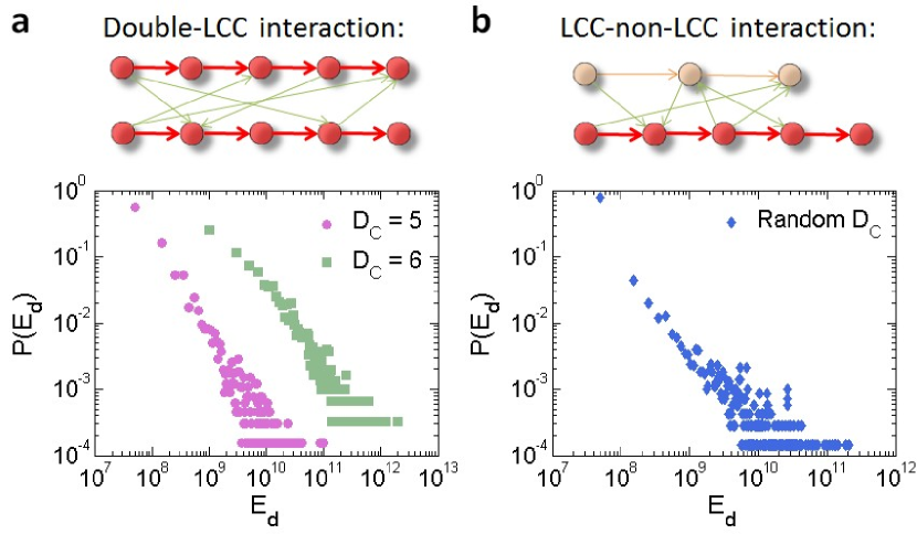
Figure A7: Distribution of control energy in a double-chain interaction models. (a) Two chains of $D_{\text{C}}=5$ (red) and $D_{\text{C}}=6$ (black), where the upper panel is a schematic illustration of two LCCs of identical length $D_{\text{C}}=5$ interacting with each other via some random links (green) between them. (b) Two chains with their lengths randomly chosen from $3-6$, where the upper panel shows the case of two interacting chains of length $5$ and $3$. The longer chain (red) plays the role of LCC, while the shorter chain is a non-LCC (orange).

Our double-chain interaction model is constructed, as follows. Consider two identical unidirectional chains, denoted by $C1$ and $C2$, each of length $D_{\text{C}}$. Every node in $C1$ connects with every node in $C2$ with probability $p$, all links between the two chains are unidirectional. A link points to $C2$ from $C1$ with probability $p_{1\rightarrow 2}$ and the probability for a link in the opposite direction is $p_{2\rightarrow 1}=1-p_{1\rightarrow 2}$. By changing the connection rate $p$ and the directional bias $p_{1\rightarrow 2}$, we can simulate and characterize various interaction patterns between the two chains. To be concrete, we generate an ensemble of 10000 interacting double-chain networks, each with $2\cdot D_{\text{C}}$ nodes and multiple randomized interchain links as determined by the parameters $p$ and $p_{1\rightarrow 2}$. As shown in Fig. A7(a), the distribution of the control energy displays a remarkable similarity to that for random networks, in that a power-law scaling behavior emerges with the exponent about $1.5$. A striking result is that the energy distributions from the double-chain interaction model are much more smooth than those from the LCC-skeleton model, indicating the key role played by the interchain interactions in spreading out the control energies that are clustered when the interactions are absent. The power-law distribution holds robustly with respect to variations in the parameters $p$ and $p_{1\rightarrow 2}$. In addition, to reveal the role of the interaction between an LCC and a non-LCC chain in the control energy, we randomly pick their lengths from $[3,6]$ with equal probability, where the longer chain acts as an LCC. Again, we observe a strong similarity between the energy distributions from random networks and from this model, as shown in Fig. A7(b), suggesting a universal pattern followed by pair interactions, regardless of the length of the chains. In particular, interactions between two chains, LCC or not, have similar effect on the control-energy distribution. These results indicate that the double-chain interaction model captures the essential physical ingredients of the energy distribution in controlling complex networks.

Appendix F: The practical controllability of real-world networks

Table A1 lists the names and types of the real-world networks studied and Table A2 presents more detailed information about the controllability of the $18$ real-world networks analyzed in the main text.

Table A1: Description of the 18 real-world networks used in the paper ($N$ - number of nodes; $M$ - number of edges).

Type Index Name $N$ $M$ Description Trust 1 College Student Duijn et al. (2003); Milo et al. (2004) 32 96 Social network 2 Prison Inmate Duijn et al. (2003); Milo et al. (2004) 67 182 Social network Circuits 3 s208a Milo et al. (2002) 122 189 Logic circuit 4 s420a Milo et al. (2002) 252 399 Logic circuit 5 s838a Milo et al. (2002) 512 189 Logic circuit Citation 6 Small World Watts and Strogatz (1998) 233 1988 Stanley Milgram 7 Kohonen Davis and Hu (2011) 3772 96 T. Kohonen Protein 8 Protein-1 Milo et al. (2004) 95 213 Protein network 9 Protein-2 Milo et al. (2004) 53 123 Protein network 10 Protein-3 Milo et al. (2004) 99 212 Protein network Food Web 11 St. Martin Baird et al. (1998) 45 224 Food Web 12 Seagrass Christian and Luczkovich (1999) 49 226 Food Web 13 Grassland Dunne et al. (2002) 88 137 Food Web 14 Ythan Dunne et al. (2002) 135 601 Food Web 15 Silwood Memmott et al. (2000) 154 370 Food Web 16 Little Rock Martinez (1991) 183 2494 Food Web 17 Baydry Ulanowicz and DeAngelis (2005) 128 2137 Food Web 18 Florida Ulanowicz and DeAngelis (2005) 128 2106 Food Web

Table A2: Practical controllability of real-world networks studied in Ref. Liu et al. (2011), where $N_{\text{D}}$ denotes the number of controllers as determined by the structural controllability theory and $M^{\star}$ is the number of augmented driver nodes needed to make the network practically controllable. The densities of the original driver nodes and with $M^{\star}$ augmented drivers included are $n_{\text{D}}=N_{\text{D}}/N$ and $n_{\text{D}}^{\star}=N_{\text{D}}^{\star}\left.\right/N$, respectively, where $n_{\text{D}}^{\star}$ is the new measure of controllability, and $E^{\star}$ denotes the new energy. When an additional control signal is added to the middle of each LCC [strategy (I)] so that $M^{\star}_{\text{mid}}$ extra control inputs are used, the control energy is $E^{\star}_{\text{mid}}$. We also test another strategy in which an extra control signal is applied to each of the $m$ convergent nodes of all LCCs [strategy (II)], in which $M^{\star}_{\text{end}}$ additional control inputs are used. The control energy required is denoted as $E^{\star}_{\text{end}}$. The control diameter $D_{\text{C}}$ of each network is listed in the last column. (See Table A1 in Appendix F for detailed description of the 18 networks.)

Type	Name	$N$	$N_{\text{D}}$	$M^{\star}$	$n_{\text{D}}$	$n_{\text{D}}^{\star}$	$E^{\star}$	$M^{\star}_{\text{mid}}$	$E^{\star}_{\text{mid}}$	$M^{\star}_{\text{end}}$	$E^{\star}_{\text{end}}$	$D_{\text{C}}$
Trust	Coll. Student	32	6	0	0.19	0.19	$7.9\times 10^{10}$	3	$2.5\times 10^{5}$	4	$7.3\times 10^{4}$	4
	Prison Inmate	67	9	27	0.13	0.54	$2.3\times 10^{7}$	1	$4.6\times 10^{3}$	1	$9.7\times 10^{4}$	5
Electronic Circuits	s208a	122	29	40	0.24	0.57	$2.3\times 10^{7}$	1	$3.0\times 10^{5}$	1	$4.0\times 10^{5}$	5
	s420a	252	59	71	0.23	0.52	$2.6\times 10^{6}$	11	$2.1\times 10^{5}$	10	$2.2\times 10^{5}$	4
	s838a	512	119	81	0.23	0.39	$4.1\times 10^{9}$	13	$3.1\times 10^{6}$	6	$3.7\times 10^{6}$	5
Citation	Small World	233	140	11	0.60	0.65	$2.0\times 10^{3}$	1	$1.9\times 10^{3}$	1	$1.9\times 10^{3}$	5
	Kohonen	3772	2114	413	0.56	0.67	$9.4\times 10^{4}$	49	$4.0\times 10^{4}$	37	$5.1\times 10^{4}$	3
Protein	Protein-1	95	48	19	0.51	0.71	$1.9\times 10^{10}$	7	$8.5\times 10^{2}$	5	$2.2\times 10^{3}$	3
	Protein-2	53	13	0	0.25	0.25	$3.7\times 10^{9}$	2	$9.0\times 10^{8}$	2	$1.2\times 10^{9}$	4
	Protein-3	99	22	35	0.22	0.58	$3.9\times 10^{5}$	3	$5.1\times 10^{4}$	3	$5.3\times 10^{4}$	4
Food Web	St. Martin	45	14	9	0.31	0.51	$2.7\times 10^{3}$	2	$9.2\times 10^{2}$	2	$1.5\times 10^{3}$	3
	Seagrass	49	13	7	0.27	0.41	$3.6\times 10^{3}$	3	$8.3\times 10^{2}$	2	$3.4\times 10^{3}$	3
	Grassland	88	46	0	0.52	0.52	$3.4\times 10^{5}$	1	$8.6\times 10^{4}$	1	$9.2\times 10^{4}$	4
	Ythan	135	69	14	0.51	0.62	$2.6\times 10^{3}$	4	$1.9\times 10^{3}$	2	$2.0\times 10^{3}$	3
	Silwood	154	116	12	0.75	0.83	$1.5\times 10^{4}$	3	$1.0\times 10^{3}$	2	$9.9\times 10^{2}$	3
	Little Rock	183	99	36	0.54	0.74	$5.4\times 10^{3}$	48	$3.6\times 10^{3}$	48	$3.6\times 10^{3}$	2
	Baydry	128	62	34	0.48	0.75	$1.7\times 10^{3}$	32	$9.6\times 10^{2}$	48	$9.6\times 10^{2}$	2
	Florida	128	30	69	0.23	0.77	NaN	1	NaN	1	NaN	3

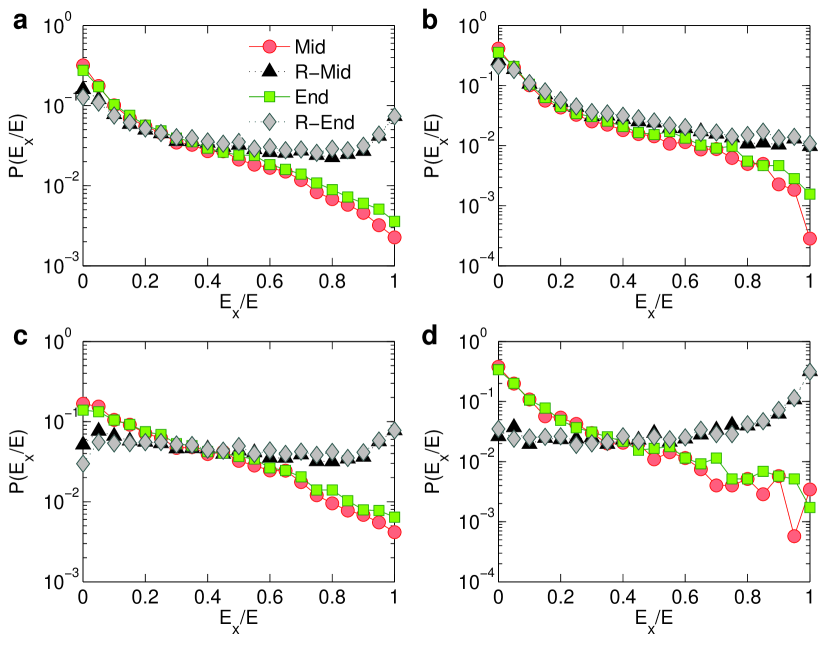
Figure A8: Effects of redundant control inputs. (a) For control diameter $D_{\text{C}}=2$, distribution of the energy ratio $E_{x}/E$ under optimization strategies (I) (Mid, red circles) and (II) (End, green squares), where $E_{x}$ and $E$ are the required energies with and without redundant control, respectively. Results from two randomized optimization strategies are marked by R-Mid (black triangles) and R-End (gray diamonds), corresponding to strategies (I) and (II), respectively. The values of $E_{x}/E$ are collected from practically controllable networks from an ensemble of $10000$ ER random networks ($\langle k\rangle=6$, $P_{\text{b}}=0.1$). For each network, if strategy (I) [or (II)] requires $r$ redundant controls, $r$ additional random control inputs are applied to the system $10$ times to average out the random fluctuations. Panels (b-d) show the $E_{x}/E$ distributions for networks with control diameter $D_{\text{C}}=3$, $4$, or $5$, respectively.

Appendix G: Energy optimization of modeled complex networks and a cascade parallel R-C circuit network

G1: Optimization strategy for modeled networks.

A realistic complex network can often have multiple LCCs, requiring multiple redundant control inputs. Say we wish to introduce a small number of extra control signals. Due to the $m$ degeneracy in the end nodes LCCs, it seems that the number of redundant control inputs should exceed $m$ if every LCC receives one such signal. However, since even a unity deduction in the LCC length can significantly lower the control energy, a simpler strategy is to place one redundant control input at each of the $m$ end-nodes to which all possible LCCs converge. In this case, each LCC in the network is broken into a chain of length $L-1$ and a single node, and consequently, the control energy is now determined by one-dimensional chains of length $L-1$ instead of length $L$. Figure A8(a) shows the effects of two optimization strategies to introduce redundant control signals on the energy distribution: applying one redundant control signal (I) at the middle and (II) at the end of each and every LCC, respectively. For comparison, for each strategy, the same number of redundant control inputs are also applied randomly throughout the network. The ratio between the control energy under optimization strategy, $E_{x}$, and the original control energy $E$ characterizes the effectiveness of the optimization strategies. In particular, if the distribution of $E_{x}/E$ is concentrated on small values of $E_{x}/E$, then the corresponding optimization strategy can be deemed to be effective. As shown in Fig. A8(a), both optimization strategies outperform the random strategies, with strategy (I) performing slightly better than (II). The networks requiring proper optimization to be practically controlled are typically those with long control diameters. Figures A8(b-d) show that this is indeed the case.

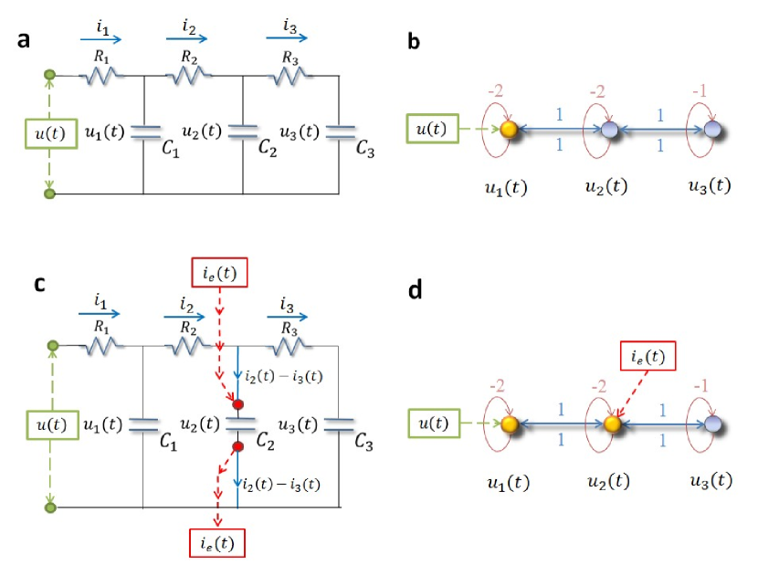
Figure A9: Controlling and optimizing a cascade parallel R-C circuit and the corresponding network presentation. (a) A cascade parallel R-C circuit with $3$ resistors ($R_{1}$, $R_{2}$, and $R_{3}$, each of resistance $1\Omega$) and $3$ capacitors ($C_{1}$, $C_{2}$, and $C_{3}$, each of capacitance $1$F), where $u(t)$ is the external input voltage, $u_{1}(t)$, $u_{2}(t)$, and $u_{3}(t)$ are the voltages on the capacitors $C_{1}$, $C_{2}$, and $C_{3}$, respectively, $i_{1}(t)$, $i_{2}(t)$, and $i_{3}(t)$ are the currents through the resistors $R_{1}$, $R_{2}$, and $R_{3}$, respectively. (b) Network representation of the circuit in (a). (c) Circuit with an extra external current input $i_{\text{e}}(t)$ into the capacitor $C_{2}$. (d) The extra external current input $i_{\text{e}}(t)$ serves as a redundant control input injected into node $2$ of the network in (b). There are two driver nodes (yellow) in the network: $1$ and $3$.

G2: An example of controlling and optimizing a circuit system.

We consider a cascade parallel R-C circuit consisting of three identical resistors and capacitors as an example to illustrate how the circuit can be abstracted into a directed network, as shown in Fig. A9. For convenience, we set $R_{1}=R_{2}=R_{3}=R$ and $C_{1}=C_{2}=C_{3}=C$, and denote the currents through $R_{1}$, $R_{2}$, and $R_{3}$ as $i_{1}(t)$ , $i_{2}(t)$, and $i_{3}(t)$, respectively. The equations of the circuit are

$$\left\{\begin{array}[]{cl}&u(t)=i_{1}(t)R+u_{1}(t)\\ &u_{1}(t)=i_{2}(t)R+u_{2}(t)\\ &u_{2}(t)=i_{3}(t)R+u_{3}(t)\\ &C\frac{\,\mathrm{d}u_{1}(t)}{\,\mathrm{d}t}=i_{1}(t)-i_{2}(t)\\ &C\frac{\,\mathrm{d}u_{2}(t)}{\,\mathrm{d}t}=i_{2}(t)-i_{3}(t)\\ &C\frac{\,\mathrm{d}u_{3}(t)}{\,\mathrm{d}t}=i_{3}(t)\end{array}\right.$$ (A43)

After some algebraic manipulation, we have

$$\left\{\begin{array}[]{cl}&\frac{\,\mathrm{d}u_{1}(t)}{\,\mathrm{d}t}=-\frac{2}{RC}u_{1}(t)+\frac{1}{RC}u_{2}(t)+\frac{1}{RC}u(t)\\ &\frac{\,\mathrm{d}u_{2}(t)}{\,\mathrm{d}t}=\frac{1}{RC}u_{1}(t)-\frac{2}{RC}u_{2}(t)+\frac{1}{RC}u_{3}(t)\\ &\frac{\,\mathrm{d}u_{3}(t)}{\,\mathrm{d}t}=\frac{1}{RC}u_{2}(t)-\frac{1}{RC}u_{3}(t),\end{array}\right.$$ (A44)

which can be written as

$$\left(\begin{array}[]{c}\frac{\,\mathrm{d}u_{1}(t)}{\,\mathrm{d}t}\\ \frac{\,\mathrm{d}u_{2}(t)}{\,\mathrm{d}t}\\ \frac{\,\mathrm{d}u_{3}(t)}{\,\mathrm{d}t}\\ \end{array}\right)=\left(\begin{array}[]{ccc}-\frac{2}{RC}&\frac{1}{RC}&0\\ \frac{1}{RC}&-\frac{2}{RC}&\frac{1}{RC}\\ 0&\frac{1}{RC}&-\frac{1}{RC}\\ \end{array}\right)\left(\begin{array}[]{c}u_{1}(t)\\ u_{2}(t)\\ u_{3}(t)\\ \end{array}\right)+\left(\begin{array}[]{c}\frac{1}{RC}\\ 0\\ 0\\ \end{array}\right)u(t).$$ (A45)

Setting $R=1\Omega$ and $C=1F$, we have

$$\left(\begin{array}[]{c}\frac{\,\mathrm{d}u_{1}(t)}{\,\mathrm{d}t}\\ \frac{\,\mathrm{d}u_{2}(t)}{\,\mathrm{d}t}\\ \frac{\,\mathrm{d}u_{3}(t)}{\,\mathrm{d}t}\\ \end{array}\right)=A\cdot\left(\begin{array}[]{c}u_{1}(t)\\ u_{2}(t)\\ u_{3}(t)\\ \end{array}\right)+B\cdot u(t),$$ (A46)

where

$$A=\left(\begin{array}[]{ccc}-2&1&0\\ 1&-2&1\\ 0&1&-1\\ \end{array}\right)$$ (A47)

is the adjacency matrix of the network representing the circuit, and

$$B=\left(\begin{array}[]{c}1\\ 0\\ 0\\ \end{array}\right)$$ (A48)

is the control input matrix. The circuit has then been transferred into a $3$-node bidirectional 1D chain network with adjacency matrix $A$.

Without loss of generality, we inject an extra external current input $i_{\text{e}}(t)$ into the capacitor $C_{2}$, and the circuit equations become:

$$\left\{\begin{array}[]{cl}&u(t)=i_{1}(t)R+u_{1}(t)\\ &u_{1}(t)=i_{2}(t)R+u_{2}(t)\\ &u_{2}(t)=i_{3}(t)R+u_{3}(t)\\ &C\frac{\,\mathrm{d}u_{1}(t)}{\,\mathrm{d}t}=i_{1}(t)-i_{2}(t)\\ &C\frac{\,\mathrm{d}u_{2}(t)}{\,\mathrm{d}t}=i_{2}(t)-i_{3}(t)+i_{\text{e}}(t)\\ &C\frac{\,\mathrm{d}u_{3}(t)}{\,\mathrm{d}t}=i_{3}(t)\end{array}\right.$$ (A49)

The state equations are

$$\left(\begin{array}[]{c}\frac{\,\mathrm{d}u_{1}(t)}{\,\mathrm{d}t}\\ \frac{\,\mathrm{d}u_{2}(t)}{\,\mathrm{d}t}\\ \frac{\,\mathrm{d}u_{3}(t)}{\,\mathrm{d}t}\\ \end{array}\right)=A\cdot\left(\begin{array}[]{c}u_{1}(t)\\ u_{2}(t)\\ u_{3}(t)\\ \end{array}\right)+B_{\text{e}}\left(\begin{array}[]{c}u(t)\\ i_{\text{e}}(t)\\ \end{array}\right),$$ (A50)

where

$$B_{\text{e}}=\left(\begin{array}[]{cc}1&0\\ 0&1\\ 0&0\\ \end{array}\right)$$ (A51)

is the control input matrix of the circuit under the original control input $u(t)$ on node $1$ and a redundant control input $i_{\text{e}}(t)$ to node $2$. Similarly, the redundant control input can be injected into any capacitor.

It is necessary to keep all other nodes unaffected while introducing exactly one extra control input into the circuit. However, any additional voltage change in any part of the circuit can lead to voltage changes on all the capacitors. A change in the current through a capacitor will not affect the currents in other components of the network, since only the time derivative of its voltage is affected. Thus, a meaningful way to introduce an extra control signal input to one node of a circuit’s network is to inject current into one particular capacitor in the circuit.

References

- Watts and Strogatz (1998) D. J. Watts and S. H. Strogatz, Nature 393, 440 (1998).
- Barabási and Albert (1999) A.-L. Barabási and R. Albert, Science 286, 509 (1999).
- Albert et al. (1999) R. Albert, H. Jeong, and A.-L. Barabási, Nature 401, 130 (1999).
- L. A. N. et al. (2000) A. L. A. N., A. Scala, M. Barthelemy, and H. E. Stanley, Proc. Natl. Acad. Sci. USA 97, 11149 (2000).
- Albert et al. (2000) R. Albert, H. Jeong, and A.-L. Barabási, Nature (London) 406, 378 (2000).
- Cohen et al. (2000) R. Cohen, K. Erez, D. Ben-Avraham, and S. Havlin, Phys. Rev. Lett. 85, 4626 (2000).
- Jeong et al. (2001) H. Jeong, S. P. Mason, A.-L. Barabási, and Z. N. Oltvai, Nature 411, 41 (2001).
- Pastor-Satorras and Vespignani (2001) R. Pastor-Satorras and A. Vespignani, Phys. Rev. Lett. 86, 3200 (2001).
- Newman et al. (2002) M. E. J. Newman, D. J. Watts, and S. H. Strogatz, Proc. Natl. Acad. Sci. USA 99, 2566 (2002).
- Albert and Barabási (2002) R. Albert and A.-L. Barabási, Rev. Mod. Phys 74, 47 (2002).
- Newman (2003) M. E. J. Newman, SIAM Rev. 45, 167 (2003).
- Palla et al. (2005) G. Palla, I. Derényi, I. Farkas, and T. Vicsek, Nature 435, 814 (2005).
- Boccaletti et al. (2006) S. Boccaletti, V. Latora, Y. Moreno, M. Chavez, and D.-U. Hwang, Phys. Rep. 424, 175 (2006).
- Caldarelli (2007) G. Caldarelli, OUP Catalogue (2007).
- Nagy et al. (2010) M. Nagy, Z. Ákos, D. Biro, and T. Vicsek, Nature 464, 890 (2010).
- Fortunato (2010) S. Fortunato, Phys. Rep. 486, 75 (2010).
- Ott et al. (1990) E. Ott, C. Grebogi, and J. A. Yorke, Phys. Rev. Lett. 64, 1196 (1990).
- Boccaletti et al. (2000) S. Boccaletti, C. Grebogi, Y.-C. Lai, H. Mancini, and D. Maza, Phys. Rep. 329, 103 (2000).
- Slotine and Li (1991) J.-J. E. Slotine and W. Li, Applied Nonlinear Control, SL:book, Vol. 199 (Prentice-Hall Englewood Cliffs, NJ, 1991).
- Wang and Chen (2002) X. F. Wang and G. Chen, Physica A 310, 521 (2002).
- Wang and Slotine (2005) W. Wang and J.-J. E. Slotine, Biol. Cyber. 92, 38 (2005).
- Sorrentino et al. (2007) F. Sorrentino, M. di Bernardo, F. Garofalo, and G. Chen, Phys. Rev. E 75, 046103 (2007).
- Yu et al. (2009) W. Yu, G. Chen, and J. Lü, Automatica 45, 429 (2009).
- Rahmani et al. (2009) A. Rahmani, M. Ji, M. Mesbahi, and M. Egerstedt, SIAM J. Cont. Opt. 48, 162 (2009).
- Egerstedt et al. (2012) M. Egerstedt, S. Martini, M. Cao, K. Camlibel, and A. Bicchi, IEEE control. Sys. 32, 66 (2012).
- Kelly et al. (1998) F. P. Kelly, A. K. Maulloo, and D. K. H. Tan, J. Oper. Res. Soc. , 237 (1998).
- Chiang et al. (2007) M. Chiang, S. H. Low, A. R. Calderbank, and J. C. Doyle, Proc. IEEE 95, 255 (2007).
- Srikant (2004) R. Srikant, The Mathematics of Internet Congestion Control, Srikant:book (Springer, 2004).
- Luenberger (1979) D. Luenberger, Introduction to dynamic systems: theory, models, and applications, Luenberger:book (Wiley, 1979).
- Kalman (1963) R. E. Kalman, J. Soc. Indus. Appl. Math. Ser. A 1, 152 (1963).
- Lin (1974) C.-T. Lin, IEEE Trans. Automat. Contr. 19, 201 (1974).
- Shields and Pearson (1975) R. W. Shields and J. B. Pearson, Rice Univ. ECE Tech. Rep. (1975).
- Reinschke and Wiedemann (1997) K. J. Reinschke and G. Wiedemann, Linear Alg. Its Appl. 266, 199 (1997).
- Sontag (1998) E. D. Sontag, Mathematical Control Theory: Deterministic Finite Dimensional Systems, Sontag:book, Vol. 6 (Springer, 1998).
- Lombardi and Hörnquist (2007) A. Lombardi and M. Hörnquist, Phys. Rev. E 75, 056110 (2007).
- Liu et al. (2011) Y.-Y. Liu, J.-J. Slotine, and A.-L. Barabási, Nature (London) 473, 167 (2011).
- Wang et al. (2012) W.-X. Wang, X. Ni, Y.-C. Lai, and C. Grebogi, Phys. Rev. E 85, 026115 (2012).
- Nepusz and Vicsek (2012) T. Nepusz and T. Vicsek, Nat. Phys. 8, 568 (2012).
- Yan et al. (2012) G. Yan, J. Ren, Y.-C. Lai, C.-H. Lai, and B. Li, Phys. Rev. Lett. 108, 218703 (2012).
- Liu et al. (2012) Y.-Y. Liu, J.-J. Slotine, and A. L. Barabási, PLoS ONE 7, e44459 (2012).
- Nacher and Akustu (2012) J. Nacher and T. Akustu, New. J. Phys. 14, 073005 (2012).
- Hopcroft and Karp (1973) J. E. Hopcroft and R. M. Karp, SIAM J. Comput. 2, 225 (1973).
- Zhou and Ou-Yang (2003) H. Zhou and Z.-C. Ou-Yang, arXiv preprint cond-mat/0309348 (2003).
- Zdeborová and Mézard (2006) L. Zdeborová and M. Mézard, J. Stat. Mech. 2006, P05003 (2006).
- Menichetti et al. (2014) G. Menichetti, L. Dall’sta, and G. Bianconi, IEEE Trans. Autom. Contr. 58, 1719 (2014).
- Wuchty (2014) S. Wuchty, ACM Transactions on Mathematical Software (TOMS) 111, 7156 (2014).
- Hautus (1969) M. L. J. Hautus, in Ned. Akad. Wetenschappen, Proc. Ser. A, Vol. 72 (Elsevier, 1969) pp. 443–448.
- Yuan et al. (2013) Z.-Z. Yuan, C. Zhao, Z.-R. Di, W.-X. Wang, and Y.-C. Lai, Nat. Commun. 4, 2447 (2013).
- Rugh (1996) W. J. Rugh, Linear System Theory, Rugh:book (Prentice-Hall, Inc., 1996).
- Chen (1984) C. T. Chen, Linear System Theory and Design, 1st ed. (Oxford University Press, Inc., 1984).
- Erdös and Rényi (1959) P. Erdös and A. Rényi, Publ. Math. 6, 290 (1959).
- Erdős and Rényi (1960) P. Erdős and A. Rényi, Publ. Math. Inst. Hung. Acad. Sci 5, 17 (1960).
- Sun and Motter (2013) J. Sun and A. E. Motter, Phys. Rev. Lett. 110, 208701 (2013).
- Strang (1976) G. Strang, Linear Algebra and Its Applications, Strang:book (Academic Press, 1976).
- Duijn et al. (2003) M. A. J. V. Duijn, M. Huisman, F. N. Stokman, F. W. Wasseur, and E. P. H. Zeggelink, J. Math. Sociol 27, 153 (2003).
- Milo et al. (2004) R. Milo, S. Itzkovitz, N. Kashtan, R. Levitt, S. Shen-Orr, I. Ayzenshtat, M. Sheffer, and U. Alon, Science 303, 1538 (2004).
- Milo et al. (2002) R. Milo, S. Shen-Orr, S. Itzkovitz, N. Kashtan, D. Chklovskii, and U. Alon, Science 298, 824 (2002).
- Davis and Hu (2011) T. A. Davis and Y. Hu, ACM Trans. Math. Software (TOMS) 38, 1 (2011).
- Baird et al. (1998) D. Baird, J. Luczkovich, and R. R. Christian, Estuarine Coast. Shelf Sci. 47, 329 (1998).
- Christian and Luczkovich (1999) R. R. Christian and J. J. Luczkovich, Ecol. Modelling 117, 99 (1999).
- Dunne et al. (2002) J. A. Dunne, R. J. Williams, and N. D. Martinez, Proc. Natl. Acad. Sci. 99, 12917 (2002).
- Memmott et al. (2000) J. Memmott, N. D. Martinez, and J. E. Cohen, J. Animal Ecol. 69, 1 (2000).
- Martinez (1991) N. D. Martinez, Ecol. Mono. 61, 367 (1991).
- Ulanowicz and DeAngelis (2005) R. E. Ulanowicz and D. L. DeAngelis, US Geo. Sur. Prog. South Florida Ecosystem 114 (2005).