Modulation Classification for MIMO-OFDM Signals via Approximate Bayesian Inference

Abstract

The problem of modulation classification for a multiple-antenna (MIMO) system employing orthogonal frequency division multiplexing (OFDM) is investigated under the assumption of unknown frequency-selective fading channels and signal-to-noise ratio (SNR). The classification problem is formulated as a Bayesian inference task, and solutions are proposed based on Gibbs sampling and mean field variational inference. The proposed methods rely on a selection of the prior distributions that adopts a latent Dirichlet model for the modulation type and on the Bayesian network formalism. The Gibbs sampling method converges to the optimal Bayesian solution and, using numerical results, its accuracy is seen to improve for small sample sizes when switching to the mean field variational inference technique after a number of iterations. The speed of convergence is shown to improve via annealing and random restarts. While most of the literature on modulation classification assume that the channels are flat fading, that the number of receive antennas is no less than that of transmit antennas, and that a large number of observed data symbols are available, the proposed methods perform well under more general conditions. Finally, the proposed Bayesian methods are demonstrated to improve over existing non-Bayesian approaches based on independent component analysis and on prior Bayesian methods based on the ‘superconstellation’ method.

I Introduction

Cognitive radio is a wireless communication technology that addresses the inefficiency of the radio resource usage via computational intelligence [1, 2]. Cognitive radios have both civilian and military applications [3]. A major task in such radios is the classification of the modulation format of unknown received signals. As the pairing of multiple-antenna (MIMO) transmission and orthogonal frequency division multiplexing (OFDM) data modulation has become central to fourth generation (4G) and fifth generation (5G) wireless technologies, a need has arisen for the development of new classification algorithms capable of handling MIMO-OFDM signals.

Modulation classification methods are generally classified as inference-based or pattern recognition-based [3]. The inference-based approaches fall into two categories, namely Bayesian and non-Bayesian methods [4]. Bayesian methods model unknown parameters as random variables with some prior distributions, and aim to evaluate the posterior probability of the modulation type. Non-Bayesian methods, instead, model unknown parameters as nuisance variables that need to be estimated before performing modulation classification. With pattern recognition-based methods, specific features are extracted from the received signal and then used to discriminate among the candidate modulations. Compared to the pattern recognition-based approaches, inference-based methods generally achieve better classification performance at the cost of a higher computational complexity [3].

There is ample literature on classification algorithms for single-antenna (SISO) systems [3], [5]-[20]. Among them, a Bayesian method using Gibbs sampling is proposed in [19]. In [20], a systematic Bayesian solution based on the latent Dirichlet Bayesian Network (BN) is proposed, which generalizes and improves upon the work in [19]. A preprocessor for modulation classification is developed in [21], whereby the timing offset is estimated using grid-based Gibbs sampling. We note that, while most algorithms rely on the assumption that the channels are flat fading or additive white Gaussian noise channels, the approaches in [19]-[21] are well-suited also for frequency selective fading channels.

Only few publications address modulation classification in MIMO systems [22]-[26]. The task of modulation classification for MIMO is more challenging than for SISO due to the mutual interference between the received signals and to the multiplicity of unknown channels. In [22], a non-Bayesian approach, referred to as independent component analysis (ICA)-phase correction (PC), is proposed, where the channel matrix required for the calculation of the hypotheses test is estimated blindly by ICA [27]. Several related pattern recognition-based algorithms are introduced in [23]-[25], where source streams are separated by ICA-PC or a constant modulus algorithm, and diverse higher-order signal statistics are used as discriminating features. Moreover, a pattern recognition-based algorithm using spatial and temporal correlation functions as distinctive features is reported in [26] for MIMO frequency-selective channels with time-domain transmission. The approach is not applicable to modulation classification for MIMO-OFDM systems. As for MIMO-OFDM systems, a non-Bayesian approach is proposed in [28] based on ICA-PC and an assumed invariance of the frequency-domain channels across the coherence bandwidth. It is finally noted that the results in this paper were partially presented in [29].

Main Contributions: In this work, we develop Bayesian modulation classification techniques for MIMO-OFDM systems operating over frequency-selective fading channels, assuming unknown channels and signal-to-noise ratio (SNR). Our main contributions are as follows.

1. A modulation classification technique is proposed based on Gibbs sampling for MIMO-OFDM systems. Inspired by the latent Dirichlet models in machine learning [30], this approach leverages a novel selection of the prior distributions for the unknown variables, the modulation format and the transmitted symbols. This selection was first adopted by some of the authors in [20] for SISO systems. As compared to SISO systems, a Gibbs sampling implementation such as in [20] may have an impractically slow convergence due to the high-dimensional and multimodal distributions in MIMO systems. The strategy of annealing [31]-[33] combined with multiple random restarts [34]-[37] is hence proposed here to improve the convergence speed.

2. An alternative Bayesian solution for modulation classification in MIMO-OFDM systems that leverages mean field variational inference [38] is proposed, based on the same latent Dirichlet prior selection.

3. A hybrid approach that switches from Gibbs sampling to mean field variational inference is proposed for modulation classification in MIMO-OFDM systems. The hybrid approach is motivated by the fact that the Gibbs sampler is superior to mean field as a method for exploring the global solution space, while the mean field algorithm has better convergence speed in the vicinity of a local optima [38]-[40].

4. Extensive numerical results demonstrate that the proposed Gibbs sampling method converges to an effective solution, and its accuracy improves for small sample sizes when switching to the mean field variational inference technique after a number of iterations. Moreover, the speed of convergence is seen to be generally improved by multiple random restarts and annealing [31]-[37]. Overall, while most of the reviewed existing modulation classification algorithms for MIMO-OFDM systems work under the assumptions that the channels are flat fading [22]-[25], that the number of receive antennas is no less than the number of transmit antennas [22]-[25], and/or that the number of samples is large (as for pattern recognition-based methods) [23]-[26], the proposed method achieves satisfactory performance under more general conditions.

The rest of the paper is organized as follows. The signal model is introduced in Sec. II. In Sec. III, we briefly review some necessary preliminary concepts, including Bayesian inference and BNs, while in Sec. IV, we formulate the modulation classification problem under study as a Bayesian inference task, and propose solutions based on Gibbs sampling and on mean field variational inference. Numerical results of the proposed methods are presented in Sec. V. Finally, conclusions are drawn in Sec. VI.

Notation: The superscripts $T$ and $H$ denote matrix or vector transpose and Hermitian, respectively. The $i$-th row of the matrix $\mathbf{B}$ is denoted as $\mathbf{B}_{(i,\cdot)}$ and the $j$-th column is denoted as $\mathbf{B}_{(\cdot,j)}$. Lower case bold letters and upper case bold letters are used to denote column vectors and matrices, respectively. The notation $\mathbf{b}\diagdown b_{i}$, where $\mathbf{b}=\left[b_{1},...,b_{n}\right]^{T}$ and $i\in\{1,...,n\}$, denotes the vector composed of all the elements of $\mathbf{b}$ except $b_{i}$. We use an angle bracket $\langle\cdot\rangle_{\centerdot}$ to represent the expectation with respect to the random variables indicated in the subscript. For notational simplicity, we do not indicate the variables in the subscript when the expectation is taken with respect to all the random variables inside the bracket $\langle\cdot\rangle_{\centerdot}$ The notations $\psi(\cdot)$ and $\mathrm{\mathbf{1}}(\cdot)$ stand for the digamma function [41] and the indicator function, respectively. The cardinality of a set $\mathcal{B}$ is denoted $\left|\mathcal{B}\right|$. We use the same notation, $p(\cdot)$, for both probability density functions (pdf) and probability mass function (pmf). Moreover, we will identify a pdf or pmf by its arguments, e.g., $p(X|Y)$ represents the distribution of random variable $X$ given the random variable $Y$. The notations $\mathcal{CN}(\mathbf{\boldsymbol{\mu}},\mathbf{C})$ and $\mathcal{IG}\left(a,b\right)$ represent the the circularly symmetric complex Gaussian distribution with mean vector $\boldsymbol{\mu}$ and covariance matrix $\mathbf{C}$ and the inverse gamma distribution with shape parameter $a$ and scale parameter $b$, respectively.

II System Model

Consider a MIMO-OFDM system operating over a frequency-selective fading channel with $N$ subcarriers, $M_{t}$ transmit antennas, $M_{r}$ receive antennas and a coherence period of $K$ OFDM symbols. All frequency-domain symbols transmitted during the coherence period are taken from a finite constellation $A\in\mathcal{A}$, such as $M$-PSK or $M$-QAM, where $\mathcal{A}$ is the (finite) set containing all possible constellations. Without loss of generality, $A$ is assumed to be a constellation of symbols with average power equal to 1. The number of transmit antennas $M_{t}$ is assumed known. We observe that several algorithms have been proposed for the estimation of $M_{t}$ [42, 43]. We focus on the problem of detecting the constellation $A$ in the absence of information about the SNR, the transmitted symbols and the fading channel coefficients.

After matched filtering and sampling, assuming that time synchronization has been successfully performed at least within the error margin afforded by the cyclic prefix, the frequency-domain samples $\mathbf{y}[n,k]=[y_{1}[n,k],...,y_{M_{r}}[n,k]]^{T}$, received across the $M_{r}$ receive antennas, at the $n$-th subcarrier of the $k$-th OFDM frame, are expressed as

$$\mathbf{y}[n,k]=\mathbf{H}[n]\mathbf{s}[n,k]+\mathbf{z}[n,k],$$ (1)

where $\mathbf{H}[n]$ is the $M_{r}\times M_{t}$ frequency-domain channel matrix associated with the $n$-th subcarrier; $\mathbf{s}[n,k]$ is the $M_{t}\times 1$ vector composed of the symbols transmitted by the $M_{t}$ antennas, i.e., $\mathbf{s}[n,k]=[s_{1}[n,k],...,s_{M_{t}}[n,k]]^{T}$, with $s_{m_{t}}[n,k]\in A$ being the symbol transmitted by the $m_{t}$-th transmit antenna over the $n$-th subcarrier of the $k$-th OFDM symbol; and $\mathbf{z}[n,k]=[z_{1}[n,k],...,z_{M_{r}}[n,k]]^{T}\sim\mathcal{CN}(\mathbf{0},\sigma^{2}\mathbf{I})$ is complex white Gaussian noise, which is independent over indices $n$ and $k$. The frequency-domain channel matrix $\mathbf{H}[n]$ can be written

$$\mathbf{H}[n]=\left[\begin{array}[]{ccc}\tilde{h}_{1,1}\left[n\right]&\cdots&\tilde{h}_{M_{t},1}\left[n\right]\\ \vdots&\ddots&\vdots\\ \tilde{h}_{1,M_{r}}\left[n\right]&\cdots&\tilde{h}_{M_{t},M_{r}}\left[n\right]\end{array}\right],$$ (2)

where $\tilde{\mathbf{h}}_{m_{t},m_{r}}=[\tilde{h}_{m_{t},m_{r}}\left[1\right],...,\tilde{h}_{m_{t},m_{r}}\left[N\right]]^{T}$ denotes the $N\times 1$ frequency-domain channel vector between the $m_{t}$-th transmit antenna and the $m_{r}$-th receive antenna. Assuming that the channel for any pair $(m_{t},m_{r})$ has at most $L$ symbol-spaced taps, we write $\tilde{\mathbf{h}}_{m_{t},m_{r}}=\mathbf{\mathbf{W}}\mathbf{h}_{m_{t},m_{r}}$, with $\boldsymbol{\mathbf{h}}_{m_{t},m_{r}}$ the $L\times 1$ time-domain channel vector and $\mathbf{W}$ the $N\times L$ matrix composed of the first $L$ columns of the DFT matrix of size $N$. Note that the channel is fixed within the coherence frame of $K$ OFDM symbols.

According to (1) and (2), the $NK\times 1$ received frequency-domain signals $\mathbf{y}_{m_{r}}=[\mathbf{y}_{m_{r}}[1]^{T},...,$$\mathbf{y}_{m_{r}}[K]^{T}]^{T}$ at the $m_{r}$-th receive antenna is given by

$$\mathbf{y}_{m_{r}}=\sum_{m_{t}=1}^{M_{t}}\mathbf{D}_{m_{t}}\tilde{\mathbf{h}}_{m_{t},m_{r}}+\mathbf{z}_{m_{r}},\>m_{r}=1,...,M_{r},$$ (3)

where $\mathbf{y}_{m_{r}}[k]=[y_{m_{r}}[1,k],...,y_{m_{r}}[N,k]]^{T}$; $\mathbf{D}_{m_{t}}=[\mathbf{D}_{m_{t},1},...,\mathbf{D}_{m_{t},K}]^{T}$ is an $NK\times N$ matrix representing the transmitted symbols with $\mathbf{D}_{m_{t},k}$ an $N\times N$ diagonal matrix whose $(n,n)$ element is $s_{m_{t}}[n,k]$; and $\mathbf{z}_{m_{r}}=[\mathbf{z}_{m_{r}}[1]^{T},...,\mathbf{z}_{m_{r}}[K]^{T}]^{T}$ with $\mathbf{z}_{m_{r}}[k]=[z_{m_{r}}[1,k],...,z_{m_{r}}[N,k]]^{T}$.

Let us further define the $NKM_{t}\times 1$ vector $\mathbf{s}=[\mathbf{s}_{1},..,\mathbf{s}_{K}]^{T}$ containing all the transmitted symbols with $\mathbf{s}_{k}=[\mathbf{s}[1,k]^{T},...,\mathbf{s}[N,k]^{T}]^{T}$; the $LM_{t}M_{r}\times 1$ vector $\mathbf{h}=[\mathbf{h}_{1}^{T},...,\mathbf{h}_{M_{r}}^{T}]^{T}$ for the time domain channels associated with all the transmit-receive antenna pairs, where $\mathbf{h}_{m_{r}}=[\boldsymbol{\mathbf{h}}_{1,m_{r}}^{T},...,\boldsymbol{\mathbf{h}}_{M_{t},m_{r}}^{T}]^{T}$; and the $NKM_{r}\times 1$ receive signal vector $\mathbf{y}=[\mathbf{y}_{1}^{T},...,\mathbf{y}_{M_{r}}^{T}]^{T}$. The task of modulation classification is for the receiver to correctly detect the modulation format $A$ given only the received samples $\mathbf{y}$, while being uninformed about the symbols $\mathbf{s}$, the channel $\mathbf{h}$ and the noise power $\sigma^{2}$. Using (1) and (3), the likelihood function $p\left(\mathbf{y}|A,\mathbf{s},\mathbf{h}\mathrm{,\sigma^{2}}\right)$ of the observation is given by

$$p\left(\mathbf{y}\Big{|}A,\mathbf{s},\mathbf{h}\mathrm{,\sigma^{2}}\right)$$

$$= \prod_{n,k}p\left(\mathbf{y}[n,k]\Big{|}\mathbf{s}[n,k],\mathbf{H}[n],\sigma^{2}\right)$$

$$= \prod_{m_{r}}p\left(\mathbf{y}_{m_{r}}\Big{|}\mathbf{s},\mathbf{h}_{m_{r}}\mathrm{,\sigma^{2}}\right),$$ (4)

with $\mathbf{y}_{m_{r}}|(\mathbf{s},\mathbf{h}_{m_{r}}\mathrm{,\sigma^{2}})$ $\sim$ $\mathcal{CN}(\sum_{m_{t=1}}^{M_{t}}\mathbf{D}_{m_{t}}\mathbf{\mathbf{W}}\mathbf{h}_{m_{t},m_{r}},\sigma^{2}\mathbf{I})$ and $\mathbf{y}[n,k]|(\mathbf{s}[n,k],\mathbf{H}[n],\sigma^{2})$ $\sim$$\mathcal{CN}(\mathbf{H}[n]\mathbf{s}[n,k],\sigma^{2}\mathbf{I})$.

III Preliminaries

As formalized in the next section, in this paper we formulate the modulation classification problem as a Bayesian inference task. In this section, we review some necessary preliminary concepts. Specifically, we start by introducing the general task of Bayesian inference in Sec. III-A; we review the definition of BN, which is a useful graphical tool to represent knowledge about the structure of a joint distribution, in Sec. III-B; and, finally, we review approximate solutions to the Bayesian inference task, namely, Gibbs sampling in Sec. III-C, and mean field variational inference in Sec. III-D.

III-A Bayesian Inference

Bayesian inference aims to compute the posterior probability of the variables of interest given the evidence, where the evidence is a subset of the random variables in the model. Specifically, given the values of some evidence variables $\mathbf{\Theta}_{e}=\mathbf{\mathbf{\boldsymbol{\theta}}}_{e}$, one wishes to estimate the posterior distribution of a subset of the unknown variables $\mathbf{\Theta}_{u}=[\Theta_{1},...,\Theta_{G}]^{T}$. We assume here for simplicity of exposition that all variables are discrete with finite cardinality. However, the extension to continuous variables with pdfs is immediate, as it will be argued. The conditional pmf of $\mathbf{\Theta}_{u}$ given the evidence $\mathbf{\Theta}_{e}=\mathbf{\mathbf{\boldsymbol{\theta}}}_{e}$ is proportional to the product of a prior distribution $p(\mathbf{\Theta}_{u})$ on the unknown variables $\mathbf{\Theta}_{u}$ and of the likelihood of the evidence $p(\mathbf{\Theta}_{e}|\mathbf{\Theta}_{u})$:

$$p(\mathbf{\Theta}_{u}|\mathbf{\Theta}_{e}=\mathbf{\boldsymbol{\theta}}_{e})\propto p(\mathbf{\Theta}_{u})p(\mathbf{\Theta}_{e}=\mathbf{\mathbf{\boldsymbol{\theta}}}_{e}|\mathbf{\Theta}_{u}).$$ (5)

If one is interested in computing the posterior distribution of the unknown variable $\Theta_{j}$, then a direct approach would be to write

$$p(\Theta_{j}=\mathbf{\theta}_{j}|\mathbf{\Theta}_{e}=\mathbf{\boldsymbol{\theta}}_{e})=\sum_{\mathbf{\boldsymbol{\theta}}_{u}\diagdown\mathbf{\theta}_{j}}p(\mathbf{\Theta}_{u}=\mathbf{\boldsymbol{\theta}}_{u}|\mathbf{\Theta}_{e}=\mathbf{\boldsymbol{\theta}}_{e}).$$ (6)

The inference task (6) is made difficult in practice by the multidimensional summation over all the values of the variables $\mathbf{\Theta}_{u}\diagdown\Theta_{j}$. Note also that, if the variables are continuous, the operation of summation is replaced by integration and a similar discussion applies. Next, we discuss the BN model.

III-B Bayesian Network

A BN is an acyclic graph that can be used to represent useful aspects of the structure of a joint distribution. Each node in the graph represents a random variable, while the directed edges between the nodes encode the probabilistic influence of one variable on another. Node $\Theta_{i}$ is defined to be a parent of $\Theta_{j}$, if an edge from node $\Theta_{i}$ to node $\Theta_{j}$ exists in the graph. According to the BN’s chain rule [38], the influence encoded in a BN for a set of variables $\mathbf{\Theta}=[\Theta_{1},...,\Theta_{J}]^{T}$ can be interpreted as the factorization of the joint distribution in the form

$$p\left(\mathbf{\Theta}\right)=\prod_{j=1}^{J}p\left(\Theta_{j}|\mathrm{P}\mathrm{a}_{\Theta_{j}}\right),$$ (7)

where we use $\mathrm{P}\mathrm{a}_{\Theta_{j}}$ to denote the set of parent variables of variable $\Theta_{j}$. Note that (7) encodes the fact that each variable $\Theta_{j}$ is independent of its ancestors in the BN, when conditioning on its parent variables $\mathrm{P}\mathrm{a}_{\Theta_{j}}$. In the following, we will find it useful to rewrite (7) in a more abstract way as [38]

$$p\left(\mathbf{\Theta}\right)=\prod_{\phi}\phi\left(\mathcal{B}_{\phi}\right),$$ (8)

where the product is taken over all $J$ factor $\phi(\mathcal{B}_{\phi})=p(\Theta_{j}|\mathrm{P}\mathrm{a}_{\Theta_{j}})$ with $\mathcal{B}_{\phi}=\{\Theta_{j},\mathrm{P}\mathrm{a}_{\Theta_{j}}\}$.

III-C Gibbs Sampling

Markov chain Monte Carlo (MCMC) techniques provide effective iterative approximate solutions to the Bayesian inference task (6) that are based on randomization and can obtain increasingly accurate posterior distributions as the number of iterations increases. The goal of these techniques is to generate $M$ random samples $\mathbf{\boldsymbol{\theta}}_{u}^{\left(1\right)},...,\mathbf{\mathbf{\boldsymbol{\theta}}}_{u}^{\left(M\right)}$ from the desired posterior distribution $p(\mathbf{\Theta}_{u}|\mathbf{\Theta}_{e}=\mathbf{\boldsymbol{\theta}}_{e})$. This is done by running a Markov chain whose equilibrium distribution is $p(\mathbf{\Theta}_{u}|\mathbf{\Theta}_{e}=\mathbf{\boldsymbol{\theta}}_{e})$. As a result, according to the law of large numbers, the multidimensional summation (or integration) (6) can be approximated by an ensemble average. In particular, the marginal distribution of any particular variable $\Theta_{j}$ in $\mathbf{\Theta}_{u}$ can be estimated as

$$p\left(\Theta_{j}=\theta_{j}|\mathbf{\Theta}_{e}=\mathbf{\boldsymbol{\theta}}_{e}\right)\approx\frac{1}{M}\sum_{m=M_{0}+1}^{M}\mathrm{\mathbf{1}}\left(\mathbf{\theta}_{j}^{\left(m\right)}=\theta_{j}\right),$$ (9)

where $\mathbf{\theta}_{j}^{\left(m\right)}$ is the $m$-th sample for $\Theta_{j}$ generated by the Markov chain, and $M_{0}$ denotes the number of samples used as burn-in period to reduce the correlations with the initial values [35].

Gibbs sampling is a classical MCMC algorithm that defines the aforementioned Markov chain by sampling all the variables in $\mathbf{\Theta}_{u}$ one-by-one. Specifically, the algorithm begins with a set of arbitrary feasible values for $\mathbf{\Theta}_{u}$. Then, at step $m$, a sample for a given variable $\Theta_{j}$ is drawn from the conditional distribution $p(\Theta_{j}|\mathbf{\Theta}_{u}\diagdown\Theta_{j},\mathbf{\Theta}_{e})$. Whenever a sample is generated for a variable, the value of that variable is updated within the vector $\mathbf{\Theta}_{u}$. It can be shown that the required conditional distributions $p(\Theta_{j}|\mathbf{\Theta}_{u}\diagdown\Theta_{j},\mathbf{\Theta}_{e})$ may be calculated by multiplying all the factors in the factorization (8) that contain the variable of interest and then normalizing the resulting distribution, i.e., we have

$$p(\Theta_{j}|\mathbf{\Theta}_{u}\diagdown\Theta_{j},\mathbf{\Theta}_{e})\propto\prod_{\phi:\,\Theta_{j}\in B_{\phi}}\phi\left(\mathcal{B}_{\phi}\right),$$ (10)

where the right-hand side of (10) is the product of the factors in (8) that involve the variable $\Theta_{j}$.

Remark 1: In order for Markov chain Monte Carlo algorithms to converge to a unique equilibrium distribution, the associated Markov chain needs to be irreducible and aperiodic [38, Ch. 12]. In the context of the Gibbs sampling, a sufficient condition for asymptotic correctness of Gibbs sampling is that the distributions $p(\Theta_{j}|\mathbf{\Theta}_{u}\diagdown\Theta_{j},\mathbf{\Theta}_{e})$ are strictly positive in their domains for all $j$.

Remark 2: When applying Gibbs sampling to practical problems, in particular those with high-dimensional and multimodal posterior distribution $p(\Theta_{j}|\mathbf{\Theta}_{u}\diagdown\Theta_{j},\mathbf{\Theta}_{e})$, slow convergence may be encountered due to the local nature of the updates. One approach to address this issue is to run Gibbs sampling with multiple random restarts that are initialized with different feasible solutions [34]-[37]. Moreover, within each run, simulated annealing may be used to avoid low-probability “traps.” Accordingly, the prior probability, or the likelihood, may be parametrized by a temperature parameter $T$, such that a large temperature implies a lower reliance on the evidence aimed at exploring more thoroughly the range of the variables. Samples are generated, starting with a high temperature and ending with a low temperature [31]-[33].

III-D Mean Field Variational Inference

Mean field variational inference provides an alternative way to approach the Bayesian inference problem of calculating $p(\Theta_{j}=\mathbf{\theta}_{j}|\mathbf{\Theta}_{e}=\mathbf{\boldsymbol{\theta}}_{e})$. The key idea of this method is that of searching for a distribution $q(\mathbf{\Theta}_{u})$ that is closest to the desired posterior distribution $p(\mathbf{\Theta}_{u}|\mathbf{\boldsymbol{\theta}}_{e})$, in terms of the Kullback-Leibler (KL) divergence $\mathrm{KL}\left(q(\mathbf{\Theta}_{u})||p(\mathbf{\Theta}_{u}|\mathbf{\boldsymbol{\theta}}_{e})\right)$, within the class $\mathcal{Q}$ of distributions that factorize as the product of marginals, i.e., $q(\mathbf{\Theta}_{u})=\prod_{j=1}^{G}q(\Theta_{j})$ [38, Ch. 11]. The corresponding variational problem is given as

$$\mathrm{\underset{\mathit{q}}{minimize}} \,\mathrm{KL}\left(q(\mathbf{\Theta}_{u})||p(\mathbf{\Theta}_{u}|\mathbf{\boldsymbol{\theta}}_{e})\right)$$ (11)

$$\mathrm{s.t.}\;q\in\mathcal{Q}.$$

By imposing the necessary optimality conditions for problem (11), one can prove that the mean field approximation $q(\mathbf{\Theta}_{u})$ is locally optimal only if the proportionality [38]

$$q\left(\Theta_{j}\right)\propto\exp\bigg{\{}\sum_{\phi:\,\Theta_{j}\in\mathcal{B}_{\phi}}\big{\langle}\ln\phi\left(\mathcal{B}_{\phi}\right)\big{\rangle}_{q\left(\mathcal{B}_{\phi}\diagdown\Theta_{j}\right)}\bigg{\}}$$ (12)

holds for all $j=1,..,G$, where the expectation in (12) is taken with respect to the distribution $q(\mathcal{B}_{\phi}\diagdown\Theta_{j})=q(\mathbf{\Theta}_{u})/q(\Theta_{j})$. The idea of the mean field variational inference is to solve (12) by means of fixed-point iterations (see [38] for details). It can be shown that each iteration of (12) results in a better approximation $q$ to the target distribution $p(\mathbf{\Theta}_{u}|\mathbf{\boldsymbol{\theta}}_{e})$, hence guaranteeing convergence to a local optimum of problem (11) [38, Sec. 11.5.1]. Once an approximating distribution $q(\mathbf{\Theta}_{u})$ is obtained, an approximation of the desired posterior $p(\mathbf{\Theta}_{u}|\mathbf{\boldsymbol{\theta}}_{e})$ can be obtained as $p(\mathbf{\Theta}_{u}|\mathbf{\boldsymbol{\theta}}_{e})\approx q(\mathbf{\Theta}_{u}),$ and the marginal posterior distribution may be approximated as $p(\Theta_{j}|\mathbf{\boldsymbol{\theta}}_{e})\approx q(\Theta_{j}).$

IV Bayesian Inference for Modulation Classification

In this section, we solve the problem of detecting the modulation $A\in\mathcal{A}$ by adopting a Bayesian inference formulation. First, in Sec. IV-A, we discuss the problem of selecting a proper prior distribution, and argue that a latent Dirichlet model inspired by [30] and first used for modulation classification in [20], provides an effective choice. Then, based on this prior model, we develop two solutions, one based on Gibbs sampling, in Sec. IV-B, and the other based on mean field variational inference, in Sec. IV-C.

IV-A Latent Dirichlet Bayesian Network

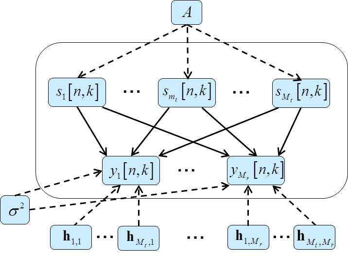
Figure 1: BN $\mathcal{G}_{1}$ for the modulation classification scheme based on the factorization (13). The nodes inside the rectangle are repeated $NK$ times.

According to (5), the joint distribution of the unknown variables $(A,\mathbf{s},\mathbf{h},\sigma^{2})$ may be expressed

$$p\left(A,\mathbf{s},\mathbf{h}\mathrm{,\sigma^{2}}\Big{|}\mathbf{y}\right)\propto p\left(\mathbf{y}\Big{|}A,\mathbf{s},\mathbf{h}\mathrm{,\sigma^{2}}\right)p\left(A,\mathbf{s},\mathbf{h}\mathrm{,\sigma^{2}}\right),$$ (13)

where the likelihood function $p\left(\mathbf{y}|A,\mathbf{s},\mathbf{h}\mathrm{,\sigma^{2}}\right)$ is given in (4), and the term $p\left(A,\mathbf{s},\mathbf{h}\mathrm{,\sigma^{2}}\right)$ stands for the prior information on the unknown quantities. The prior is assumed to factorize as

$$p\left(A,\mathbf{s},\mathbf{h}\mathrm{,\sigma^{2}}\right)= p\left(A\right)\bigg{\{}\prod_{n,k,m_{t}}p\left(s_{m_{t}}[n,k]|A\right)\bigg{\}}\cdot$$

$$\cdot\prod_{m_{t},m_{r}}p\left(\boldsymbol{\mathbf{h}}_{m_{t},m_{r}}\right)p\left(\sigma^{2}\right).$$ (14)

IV-A1 Conventional Prior

A natural choice for the prior distribution of the unknown variables $(A,\mathbf{s},\mathbf{h},\sigma^{2})$ is given by $A\sim\mathrm{uniform}\left(\mathcal{A}\right)$, $s_{m_{t}}[n,k]|A\sim\mathrm{uniform}(A)$, $\boldsymbol{\mathbf{h}}_{m_{t},m_{r}}\sim\mathcal{CN}(\mathbf{0},\alpha\mathbf{I})$, and $\sigma^{2}\sim\mathcal{IG}\left(\alpha_{0},\beta_{0}\right)$ with fixed parameters $(\alpha,\alpha_{0},\beta_{0})$ [20]. Recall that the inverse Gamma distribution is the conjugate prior for the Gaussian likelihood at hand, and that uninformative priors can be obtained by selecting sufficiently large $\alpha$ and $\beta_{0}$ and sufficiently small $\alpha_{0}$ [35]. The factorization (14) implies that, under the prior information, the variables $A$, $\boldsymbol{\mathbf{h}}_{m_{t},m_{r}}$ and $\sigma^{2}$ are independent of each other, and that the transmitted symbols $s_{m_{t}}[n,k]$ are independent of all the other variables in (14) when conditioned on the modulation $A$. The BN $\mathcal{G}_{1}$ that encodes the factorization given by (13), along with (4) and (14), is shown in Fig. 1.

The Bayesian inference task for modulation classification of MIMO-OFDM is to compute the posterior probability of the modulation $A$ conditioned on the received signal $\mathbf{y}$, namely

$$p\left(A|\mathbf{y}\right)=\sum_{\mathbf{s}}\int p\left(A\text{,}\mathbf{s},\mathbf{h\mathrm{,\sigma^{2}}}|\mathbf{y}\right)d\mathbf{h}d\sigma^{2}.$$ (15)

Following the discussion in Sec. III, the calculation in (15) is intractable because of the multidimensional summation and integration. Gibbs sampling (Sec. III-C) and mean field variational inference (Sec. III-D) offer feasible alternatives. However, the prior distribution (14) does not satisfy the sufficient condition mentioned in Remark 1, since some of the conditional distributions required for Gibbs sampling are not strictly positive in their domains. In particular, the required conditional distribution for modulation $A$ can be expressed as

$$p(A=a|\mathbf{s},\mathbf{h\mathrm{,\sigma^{2}}},\mathbf{y})\propto p\left(A\right)\prod_{n,k,m_{t}}p\left(s_{m_{t}}[n,k]|A\right).$$ (16)

The conditional distribution term $p(s_{m_{t}}[n,k]|A=a)$ in (16) is zero for all values of $s_{m_{t}}[n,k]$ not belonging to the constellation $a$, i.e., $p(s_{m_{t}}[n,k]|a)=0$ for $s_{m_{t}}[n,k]\notin a$. Therefore, the conditional distribution $p(A=a|\mathbf{s},\mathbf{h\mathrm{,\sigma^{2}}},\mathbf{y})$ is equal to zero if the transmitted symbols $\mathbf{s}$ do not belong to $a$. As a result, the Gibbs sampler may fail to converge to the posterior distribution (see, e.g., [21]). In order to alleviate the problem outlined above, we propose to adopt a prior distribution encoded on a latent Dirichlet BN $\mathcal{G}_{2}$ shown in Fig. 2.

IV-A2 Latent Dirichlet BN

Next, we introduce the Gibbs sampler based on on a latent Dirichlet BN $\mathcal{G}_{2}$ in details. Accordingly, each transmitted symbol $s_{m_{t}}[n,k]$ is distributed as a random mixture of uniform distributions on the different constellations in the set $\mathcal{A}$. Specifically, a random vector $\mathbf{p}_{A}$ of length $\left|\mathcal{A}\right|$ is introduced to represent the mixture weights, with $\mathbf{p}_{A}(a)$ being the probability that each symbol $s_{m_{t}}[n,k]$ belongs to the constellation $a\in\mathcal{A}$. Given the mixture weights $\mathbf{p}_{A}$, the transmitted symbols $s_{m_{t}}[n,k]$ are mutually independent and distributed according to a mixture of uniform distributions, i.e., $p\left(s_{m_{t}}[n,k]|\mathbf{p}_{A}\right)=\sum_{a:\,s_{m_{t}}[n,k]\in a}\mathbf{p}_{A}\left(a\right)/\left|a\right|$. The Dirichlet distribution is selected as the prior distribution of $\mathbf{p}_{A}$ in order to simplify the development of the proposed solutions, as shown in the following subsections. In particular, given a set of nonnegative parameters $\boldsymbol{\gamma}=[\gamma_{1},\cdots,\gamma_{\left|\mathcal{A}\right|}]^{T}$, we have $\mathbf{p}_{A}\sim\mathrm{Dirichlet}\left(\boldsymbol{\gamma}\right)$ [38]. We recall that the parameter $\gamma_{a}$ has an intuitive interpretation as it represents the number of symbols in constellation $a\in\mathcal{A}$ observed during some preliminary measurements.

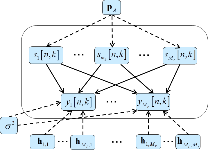
Figure 2: BN $\mathcal{G}_{2}$ for the modulation classification scheme based on the Dirichlet latent variable $\mathbf{p}_{A}$. The nodes inside the rectangle are repeated $NK$ times.

The BN $\mathcal{G}_{2}$ encodes a factorization of the conditional distribution $p(\mathbf{p}_{A},\mathbf{s},\mathbf{h}\mathrm{,\sigma^{2}}|\mathbf{y})$

$$p(\mathbf{p}_{A},\mathbf{s},\mathbf{h}\mathrm{,\sigma^{2}}|\mathbf{y})$$

$$\propto p\left(\mathbf{y}\Big{|}\mathbf{p}_{A},\mathbf{s},\mathbf{h}\mathrm{,\sigma^{2}}\right)p\left(\mathbf{p}_{A}\right)\bigg{\{}\prod_{n,k,m_{t}}p\left(s_{m_{t}}[n,k]|\mathbf{p}_{A}\right)\bigg{\}}\cdot$$

$$\cdot\prod_{m_{t},m_{r}}p\left(\boldsymbol{\mathbf{h}}_{m_{t},m_{r}}\right)p\left(\sigma^{2}\right),$$ (17)

where we have $\mathbf{p}_{A}\sim\mathrm{Dirichlet}\left(\boldsymbol{\gamma}\right)$ with a set of nonnegative parameters $\boldsymbol{\gamma}=[\gamma_{1},\cdots,\gamma_{\left|\mathcal{A}\right|}]^{T}$ [38], $p\left(s_{m_{t}}[n,k]|\mathbf{p}_{A}\right)=\sum_{a:\,s_{m_{t}}[n,k]\in a}\mathbf{p}_{A}\left(a\right)/\left|a\right|$, and the other distributions are as in (4) and (14). The Bayesian inference task for modulation classification is to compute the posterior probability of the mixture weight vector $\mathbf{p}_{A}$ conditional on the received signal $\mathbf{y}$, namely

$$p\left(\mathbf{p}_{A}|\mathbf{y}\right)=\sum_{\mathbf{s}}\int p\left(\mathbf{p}_{A}|\mathbf{s},\mathbf{h\mathrm{,\sigma^{2}}}\Big{|}\mathbf{y}\right)d\mathbf{h}d\sigma^{2},$$ (18)

and then to estimate $A$ as the value that maximize the a posteriori mean of $\mathbf{p}_{A}$:

$$\hat{A}=\arg\max_{a\in\mathcal{A}}\big{\langle}\mathbf{p}_{A}\left(a\right)\mid\mathbf{y}\big{\rangle}_{p\left(\mathbf{p}_{A}|\mathbf{y}\right)}.$$ (19)

The proposed approach guarantees that all the conditional distributions needed for Gibbs sampling based on the BN $\mathcal{G}_{2}$ are non-zero, and therefore the aforementioned convergence problem for the inference based on BN $\mathcal{G}_{1}$ is avoided.

IV-B Modulation Classification via Gibbs Sampling

In this subsection, we elaborate on Gibbs sampling for modulation classification. As explained in Sec. III-C, in order to sample from the joint posterior distribution (17), the distribution of each variable conditioned on all other variables is needed. According to (10), we have (for derivations see Appendix II):

1. The conditional distribution of the vector $\mathbf{p}_{A}$, given $\mathbf{s}$, $\mathbf{h}$, $\mathrm{\sigma^{2}}$ and $\mathbf{y}$ can be expressed as

   $$p\left(\mathbf{p}_{A}\Big{|}\mathbf{s},\mathbf{h}\mathrm{,\sigma^{2}},\mathbf{y}\right)\sim\mathrm{Dirichlet}\left(\boldsymbol{\gamma}+\mathbf{c}\right),$$ (20)

   where $\mathbf{c}=\left[c_{1},\cdots,c_{\left|\mathcal{A}\right|}\right]^{T}$, and $c_{a}$ is the number of samples of transmitted symbols in constellation $a\in\mathcal{A}$;

2. The distribution of transmitted symbols $s_{m_{t}}[n,k]$, conditioned on $\mathbf{p}_{A}$, $\mathbf{s}\diagdown s_{m_{t}}[n,k]$, $\mathbf{h}$, $\mathrm{\sigma^{2}}$ and $\mathbf{y}$, is given by

   $$p\left(s_{m_{t}}[n,k]\Big{|}\mathbf{p}_{A},\mathbf{s}\diagdown s_{m_{t}}[n,k],\mathbf{h\mathrm{,\sigma^{2},}}\mathbf{y}\right)$$

   $$\propto p\left(s_{m_{t}}[n,k]|\mathbf{p}_{A}\right)p\left(\mathbf{y}[n,k]\Big{|}\mathbf{s}[n,k],\mathbf{H}[n],\sigma^{2}\right),$$ (21)

   where we recall that when a new sample is generated for $s_{m_{t}}[n,k]$ , the new value is updated and used in computing subsequent samples in $\mathbf{s}$;

3. The required distribution for channel vector $\boldsymbol{\mathbf{h}}_{m_{t},m_{r}}$ is given by

   $$\boldsymbol{\mathbf{h}}_{m_{t},m_{r}}\Big{|}\left(\mathbf{P}_{A},\mathbf{s},\mathbf{h}\diagdown\boldsymbol{\mathbf{h}}_{m_{t},m_{r}},\mathbf{\mathrm{\sigma^{2},}}\mathbf{y}\right)$$

   $$\sim \mathcal{CN}(\hat{\mathbf{h}}_{m_{t},m_{r}},\hat{\boldsymbol{\Sigma}}_{m_{t},m_{r}}),$$ (22)

   where we have

   $$\left(\hat{\boldsymbol{\Sigma}}_{m_{t},m_{r}}\right)^{-1} =\frac{1}{\mathrm{\sigma^{2}}}\mathbf{W}^{H}\mathbf{D}_{m_{t}}^{H}\left(\mathbf{D}_{m_{t}}\mathbf{W}\right),$$ (23)

   and

   $$\hat{\mathbf{h}}_{m_{t},m_{r}}= \frac{\hat{\boldsymbol{\Sigma}}_{m_{t},m_{r}}}{\sigma^{2}}\mathbf{W}^{H}\mathbf{D}_{m_{t}}^{H}\cdot$$

   $$\cdot\bigg{(}\mathbf{y}_{m_{r}}-\sum_{m_{t}^{\prime}\neq m_{t}}\mathbf{D}_{m_{t}^{\prime}}\tilde{\mathbf{h}}_{m_{t}^{\prime},m_{r}}\bigg{)};$$ (24)

4. The conditional distribution for $\sigma^{2}$, conditioned on $\mathbf{p}_{A}$, $\mathbf{s}$, $\mathbf{h}$, and $\mathbf{y}$, is given by

   $$\sigma^{2}\Big{|}\mathbf{p}_{A}\mathbf{s},\mathbf{h},\mathbf{y}\sim\mathcal{IG}\left(\alpha,\beta\right),$$ (25)

   where $\alpha=\alpha_{0}+NKM_{r}$ and $\beta=\beta_{0}+\sum_{m_{r}}\left\|\mathbf{\mathbf{y}}_{m_{r}}-\sum_{m_{t}}\mathbf{D}_{m_{t}}\tilde{\mathbf{h}}_{m_{t},m_{r}}\right\|^{2}$. Note that (20) is a consequence of the fact that Dirichlet distribution is the conjugate prior of the categorical likelihood [38]; (22) can be derived by following from standard MMSE channel estimation results [44]; and (25) follows the fact that the inverse Gamma distribution is the conjugate prior for the Gaussian distribution [45].

We summarize the proposed Gibbs sampler for modulation classification in Algorithm 1.

Algorithm 1 Gibbs Sampling

• Initialize $\mathbf{\boldsymbol{\theta}}_{u}^{\left(0\right)}=\{\mathbf{p}_{A}^{(0)},\mathbf{s}^{(0)},\mathbf{h}\mathrm{{}^{(0)},\sigma^{2}}^{(0)}\}$ from prior distributions as discussed in Sec. IV-A

• for each iteration $m=1:\,M$

  • given $\{\mathbf{s}^{(m-1)},\mathbf{h}\mathrm{{}^{(m-1)},\sigma^{2}}^{(m-1)}\}$ draw a sample $\mathbf{p}_{A}^{(m)}$ from $p(\mathbf{p}_{A}|\mathbf{s},\mathbf{h}\mathrm{,\sigma^{2}},\mathbf{y})$ in (20);

  • given $\{\mathbf{p}_{A}^{(m)},\mathbf{h}\mathrm{{}^{(m-1)},\sigma^{2}}^{(m-1)},(\mathbf{s}\diagdown s_{m_{t}}[n,k])^{(m)}\}$, draw a sample $s_{m_{t}}^{(m)}[n,k]$ from $p(s_{m_{t}}[n,k]|\mathbf{p}_{A},\mathbf{s}\diagdown s_{m_{t}}[n,k],\mathbf{h\mathrm{,\sigma^{2},}}\mathbf{y})$ in (21);

  • given $\{\mathbf{p}_{A}^{(m)},\mathbf{s}\mathrm{{}^{(m)},\sigma^{2}}^{(m-1)},(\mathbf{h}\diagdown\boldsymbol{\mathbf{h}}_{m_{t},m_{r}})^{(m)}\}$ and the current sample values for , draw a sample $\boldsymbol{\mathbf{h}}_{m_{t},m_{r}}^{(m)}$ from $p(\boldsymbol{\mathbf{h}}_{m_{t},m_{r}}|(\mathbf{P}_{A},\mathbf{s},\mathbf{h}\diagdown\boldsymbol{\mathbf{h}}_{m_{t},m_{r}},\mathbf{\mathrm{\sigma^{2},}}\mathbf{y}))$ in (22);

  • given $\{\mathbf{p}_{A}^{(m)},\mathbf{s}^{(m)},\mathbf{h}^{(m)}\}$ draw sample $\mathrm{\sigma^{2}}^{(m)}$ from $p(\sigma^{2}|\mathbf{p}_{A}\mathbf{s},\mathbf{h},\mathbf{y})$ in (25);

• end for

Remark 3: In [19], an alternative Gibbs sampling approach based on a “superconstellation” is proposed to solve the convergence problem at hand for modulation classification in SISO. The Gibbs sampling scheme in [19] can be viewed as an approximation of the approach based on the latent Dirichlet BN obtained by setting the prior distribution $\mathbf{p}_{A}\sim\mathrm{Dirichlet}\left(\boldsymbol{\gamma}\right)$ such that $\boldsymbol{\gamma}=\mathbf{0}$ and by setting the sample value of $\mathbf{p}_{A}$ to be equal to the mean of the conditional distribution $p(\mathbf{p}_{A}|\mathbf{s},\mathbf{h}\mathrm{,\sigma^{2}},\mathbf{y})$, i.e., $\mathbf{p}_{A}^{(m)}=\mathbf{c}/\sum_{a\in A}c_{a}$ [20], where we recall that $c_{a}$ is the number of symbols that belong to constellation $a\in\mathcal{A}$. The performance of the “superconstellation” approach extended to MIMO OFDM is discussed in Sec. V.

Remark 4: When the SNR is high, the convergence speed is severely limited by the close-to-zero probabilities in the conditional distribution (21). Specifically, as the Gibbs sampling proceeds with its iterations, the samples of $\sigma^{2}$ tend to be small, making the relationship between $\mathbf{y}[n,k]$ and $s_{m_{t}}[n,k]$ almost deterministic. In particular, the term $p(\mathbf{y}[n,k]|\mathbf{s}[n,k],\mathbf{H}[n],\sigma^{2})$ in (21) satisfies $p(\mathbf{y}[n,k]|\mathbf{s}^{(m)}[n,k],\mathbf{H}^{(m)}[n],(\sigma^{2})^{(m)})\simeq 1$ for the selected sample value $\mathbf{s}^{(m)}[n,k]$ , and $p(\mathbf{y}[n,k]|\mathbf{s}^{(m)}[n,k],\mathbf{H}^{(m)}[n],(\sigma^{2})^{(m)})\simeq 0$ for all other possible values for $\mathbf{s}[n,k]$. As a result, transition between states with different values in the Markov chain occurs with a very low probability leading to extremely slow convergence. As discussed in Remark 2, the strategy of Gibbs sampling with multiple random restarts and annealing may be adopted to address this issue. For simulated annealing, we substitute the conditional distribution (25) for $\sigma^{2}$ with an iteration dependent prior given as [33]

$$\sigma^{2}\Big{|}\mathbf{p}_{A}\mathbf{s},\mathbf{h},\mathbf{y}\sim\mathcal{IG}\left(\alpha^{\prime},\beta\right),$$ (26)

where we have $\alpha^{\prime}(m)=(1-(1-p_{0})\exp(-m/m_{0}))\alpha$, with $m$ denoting the current iteration index, $p_{0}=0.1$ and $m_{0}=0.3M$, where $M$ is the total number of iterations. For multiple restarts, we propose to use the entropy of the pmf $\big{\langle}\mathbf{p}_{A}\big{\rangle}_{p\left(\mathbf{p}_{A}|\mathbf{y}\right)}$, estimated in a run as the metric, to choose among the $N_{run}$ runs of Gibbs sampling which one should be used in (19). Specifically, the run with the minimum entropy estimate $\big{\langle}\mathbf{p}_{A}\big{\rangle}_{p\left(\mathbf{p}_{A}|\mathbf{y}\right)}$ is selected. The rationale of this choice is that an estimate $\big{\langle}\mathbf{p}_{A}\big{\rangle}_{p\left(\mathbf{p}_{A}|\mathbf{y}\right)}$ with a low entropy identifies a specific modulation type with a smaller uncertainty than an estimate $\big{\langle}\mathbf{p}_{A}\big{\rangle}_{p\left(\mathbf{p}_{A}|\mathbf{y}\right)}$ with higher entropy (i.e., closer to a uniform distribution).

IV-C Modulation classification via Mean Field Variational Inference

Following the discussion in Sec. III-D, the goal of mean field variational inference applied to the problem at hand is that of searching for a distribution $q(\mathbf{p}_{A},\mathbf{s},\mathbf{h},\sigma^{2})$ that is closest to the desired posterior distribution $p(\mathbf{p}_{A},\mathbf{s},\mathbf{h},\sigma^{2}|\mathbf{y})$, in terms of the Kullback-Leibler (KL) divergence $\mathrm{KL}\left(q(\mathbf{p}_{A},\mathbf{s},\mathbf{h},\sigma^{2})||p(\mathbf{p}_{A},\mathbf{s},\mathbf{h},\sigma^{2}|\mathbf{y})\right)$, within the class $\mathcal{Q}$ of distributions that factorize as

$$q(\mathbf{p}_{A},\mathbf{s},\mathbf{h},\sigma^{2}) =q\left(\mathbf{p}_{A}\right)q\left(\mathbf{s}\right)q\left(\mathbf{h}\right)q\left(\sigma^{2}\right),$$ (27)

where $q\left(\mathbf{s}\right)=\prod_{k=1}^{K}\prod_{n=1}^{N}\prod_{m_{t}}^{M_{t}}q(s_{m_{t}}[n,k])$, and $q\left(\mathbf{h}\right)=\prod_{m_{t}}^{M_{t}}\prod_{m_{r}}^{M_{r}}\boldsymbol{\mathbf{h}}_{m_{t},m_{r}}$. Next, we present the fixed-point equations for mean field variational inference. These update equations may be derived by applying (12) to the joint pdf (17). We recall that (12) requires taking expectations of the relevant variables with respect to updated distribution $q$. If all distributions $q\left(\mathbf{p}_{A}\right)$, $q\left(\boldsymbol{\mathbf{h}}\right)$ and $q\left(\sigma^{2}\right)$ are initialized by choosing from the conjugate exponential prior family [39], [46] in a way being consistent with the priors in (17), namely $q\left(\mathbf{p}_{A}\right)$ being a Dirichlet distribution, $q\left(\boldsymbol{\mathbf{h}}\right)$ being a circularly complex Gaussian distribution, and $q\left(\sigma^{2}\right)$ being an inverse Gamma distribution, these fixed point update equations can be calculated, using a similar approach as in the Appendix I, as follows.

1. The fixed point update equation for the mixture weight vector $\mathbf{p}_{A}$ can be expressed as

   $$q\left(\mathbf{p}_{A}\right)=\mathrm{Dirichlet}\left(\boldsymbol{\gamma}+\mathbf{g}\right),$$ (28)

   where $\mathbf{g}=\left[g_{1},\cdots,g_{\left|\mathcal{A}\right|}\right]^{T}$ and $g_{a}=\sum_{n,k,m_{t}}\sum_{s_{m_{t}}[n,k]\in a}q(s_{m_{t}}[n,k])$.

2. The update equation for the transmitted symbol $s_{m_{t}}[n,k]$ is given by

   $$q\left(s_{m_{t}}[n,k]\right)\propto\exp\Big{[}\big{\langle}\ln p\left(s_{m_{t}}[n,k]|\mathbf{p}_{A}\right)\big{\rangle}_{q\left(\mathbf{p}_{A}\right)}+$$

   $$\big{\langle}\ln p\left(\mathbf{y}[n,k]|\mathbf{s}[n,k],\mathbf{H}[n],\sigma^{2}\right)\big{\rangle}_{q\left(\mathbf{s}[n,k]\diagdown s_{m_{t}}[n,k],\mathbf{h},\sigma^{2}\right)}\Big{]}$$ (29)

   where the detailed expression of (29) is shown in Appendix III.

3. The equation for the channel vector $\boldsymbol{\mathbf{h}}_{m_{t}m_{r}}$ is given by

   $$q\left(\boldsymbol{\mathbf{h}}_{m_{t}m_{r}}\right)\mathcal{=CN}(\hat{\mathbf{h}}_{m_{t},m_{r}},\hat{\boldsymbol{\Sigma}}_{m_{t},m_{r}}),$$ (30)

   where

   $$\left(\hat{\boldsymbol{\Sigma}}_{m_{t},m_{r}}\right)^{-1} =\frac{\alpha}{\beta}\mathbf{W}^{H}\big{\langle}\mathbf{D}_{m_{t}}^{H}\mathbf{D}_{m_{t}}\big{\rangle}\mathbf{W},$$ (31)

   $$\hat{\mathbf{h}}_{m_{t},m_{r}}$$

   $$= \frac{\alpha}{\beta}\mathbf{W}^{H}\big{\langle}\mathbf{D}_{m_{t}}\big{\rangle}^{H}\bigg{(}\mathbf{y}_{m_{r}}-\sum_{m_{t}^{\prime}\neq m_{t}}\mathbf{\mathbf{\Lambda}}_{m_{t}^{\prime},m_{r}}\bigg{)},$$ (32)

   $$\mathbf{\mathbf{\Lambda}}_{m_{t}^{\prime},m_{r}}=\big{\langle}\mathbf{D}_{m_{t}}\big{\rangle}\mathbf{W}\hat{\mathbf{h}}_{m_{t}^{\prime},m_{r}},$$ (33)

   and $\big{\langle}\mathbf{D}_{m_{t}}^{H}\mathbf{D}_{m_{t}}\big{\rangle}$ is a diagonal matrix whose$\left(n,n\right)$ element is equal to $\sum_{k=1}^{K}\big{\langle}|s_{m_{t}}[n,k]|^{2}\big{\rangle}$.

4. The fixed point update equation for the noise variance $\sigma^{2}$ can be expressed as

   $$q\left(\sigma^{2}\right)=\mathcal{IG}\left(\alpha,\beta\right),$$ (34)

   where $\alpha=\alpha_{0}+NKM_{r}$, and $\beta=\beta_{0}+\sum_{m_{r}}\beta_{m_{r}}$ with

   $$\beta_{m_{r}}= \left|\mathbf{y}_{m_{r}}\right|^{2}-2\mathrm{real}\bigg{[}\mathbf{y}_{m_{r}}^{H}\sum_{m_{t}}\mathbf{\Lambda}_{m_{t},m_{r}}\bigg{]}+$$

   $$+\sum_{m_{t}}\mathbf{\Psi}_{m_{t},m_{r}}+\sum_{m_{t}}\mathbf{\Xi}_{m_{t},m_{r}},$$ (35)

   $$\mathbf{\Psi}_{m_{t},m_{r}}= \mathrm{tr}\left[\mathbf{W}^{H}\big{\langle}\mathbf{D}_{m_{t}}^{H}\mathbf{D}_{m_{t}}\big{\rangle}\mathbf{W}\hat{\boldsymbol{\Sigma}}_{m_{t},m_{r}}\right]+$$

   $$\hat{\mathbf{h}}_{m_{t},m_{r}}^{H}\mathbf{W}^{H}\big{\langle}\mathbf{D}_{m_{t}}^{H}\mathbf{D}_{m_{t}}\big{\rangle}\mathbf{W}\hat{\mathbf{h}}_{m_{t},m_{r}},$$ (36)

   and

   $$\mathbf{\Xi}_{m_{t},m_{r}}=\hat{\mathbf{h}}_{m_{t},m_{r}}^{H}\mathbf{W}^{H}\big{\langle}\mathbf{D}_{m_{t}}\big{\rangle}^{H}\big{\langle}\mathbf{D}_{m_{t}^{\prime}}\big{\rangle}\mathbf{W}\hat{\mathbf{h}}_{m_{t}^{\prime},m_{r}},$$ (37)

   where we use $\mathrm{tr}[\cdot]$ to denote the trace of a matrix.

We summarize the proposed iterative mean field variational inference for modulation classification in Algorithm 2.

Algorithm 2 Mean Field Variational Inference

• Initialize $q\left(\mathbf{p}_{A}\right)$, $q\left(\mathbf{s}\right)$, $q\left(\boldsymbol{\mathbf{h}}\right)$ and $q\left(\sigma^{2}\right)$

• for each iteration $m=1:\,M$

  • given the most updated distribution $q\left(\mathbf{s}\right)$, $q\left(\boldsymbol{\mathbf{h}}\right)$ and $q\left(\sigma^{2}\right)$, update the distribution $q\left(\mathbf{p}_{A}\right)$ using (28);

  • given the most updated distribution $q\left(\mathbf{p}_{A}\right)$, $q\left(\mathbf{s}\diagdown s_{m_{t}}[n,k]\right)$, $q\left(\boldsymbol{\mathbf{h}}\right)$ and $q\left(\sigma^{2}\right)$, update the distribution $q\left(s_{m_{t}}[n,k]\right)$ using (29);

  • given the most updated distribution $q\left(\mathbf{p}_{A}\right)$, $q\left(\mathbf{s}\right)$, $q\left(\boldsymbol{\mathbf{h}}\diagdown\boldsymbol{\mathbf{h}}_{m_{t},m_{r}}\right)$ and $q\left(\sigma^{2}\right)$, update the distribution $q\left(\boldsymbol{\mathbf{h}}_{m_{t},m_{r}}\right)$ using (30);

  • given the most updated distribution $q\left(\mathbf{p}_{A}\right)$, $q\left(\mathbf{s}\right)$, and $q\left(\boldsymbol{\mathbf{h}}\right)$, update the distribution $q\left(\sigma^{2}\right)$ according to (34);

• end for

Remark 5: While Gibbs sampler is generally known to be superior to mean field as a method for exploring the global solution space, the mean field algorithm is known to have better convergence speed in the vicinity of a local optima [38], [39], [40]. Following [39], we then propose a hybrid strategy strategy that switches from Gibbs sampling to mean field variational inference to “zoom in” on the local minimum of the optimization problem (11). Additional discussion on this point can be found in the next section. A break-down of the contribution to the computational complexity of each iteration for the proposed Gibbs sampler are shown in Table I. In summary, the Gibbs sampler requires $\mathcal{O}\{N_{it}M_{t}M_{r}[NK(NL+L^{2}+M_{t}N+M_{t}M_{\mathcal{A}})+L^{3}]\}$ basic arithmetic operations, where $N_{it}$ is the total number of iterations and $M_{\mathcal{A}}$ is the total number of states of all possible constellations, i.e., $M_{\mathcal{A}}=\sum_{a\in\mathcal{A}}\left|a\right|$. At each iteration, the number of the basic arithmetic operations required for mean field variational inference is of the same order of magnitude as that for Gibbs sampling. This similarity of the computational complexity of Gibbs sampling and mean field variational inference is also reported in [39], [40] and [47].

Table I: Computational Complexity for Gibbs sampling

Unknowns	Computational complexity for sampling the variable
$\mathbf{p}_{A}$	$\mathcal{O}\{NK\}$
$\mathbf{s}$	$\mathcal{O}\{M_{t}^{2}M_{r}NKM_{\mathcal{A}}\}$
$\mathbf{h}$	$\mathcal{O}\{M_{t}M_{r}[NK(NL+L^{2}+M_{t}N)+L^{3}]\}$
$\sigma^{2}$	$\mathcal{O}\{M_{t}M_{r}N^{2}K\}$
Total	$\mathcal{O}\{N_{it}M_{t}M_{r}[NK(NL+L^{2}+M_{t}N+M_{t}M_{\mathcal{A}})+L^{3}]\}$

V Numerical Results and Discussions

In this section, we evaluate the performance of the proposed modulation classification schemes for the detection of three possible modulation formats within a MIMO-OFDM system. The performance criterion is the probability of correct classification assuming that all the modulations are equally likely. Normalized Rayleigh fading channels are assumed such that $E[\left\|\mathbf{h}_{m_{t},m_{r}}\right\|^{2}]=1.$ We define the average SNR as $10\log(M_{t}/\mathrm{\sigma^{2})}$. Unless stated otherwise, the following conditions are assumed: i) $\mathcal{A}$={QPSK, 8-PSK, 16QAM}; ii) $M_{t}=M_{r}=2$ antennas; iii) $K=2$ OFDM symbols; and iv) $L=5$ taps with relative powers given by $[0\mathrm{\,dB},-4.2\mathrm{\,dB},-11.5\,\mathrm{dB},-17.6\mathrm{\,dB},$ $-21.5\,\mathrm{dB}]$.

V-A Performance of Gibbs Sampling

V-A1 Gibbs Sampling with Restarts and Annealing

We first investigate the performance of the proposed Gibbs sampling algorithms with or without multiple random restarts and simulated annealing within each run (see Remark 4). The number of runs in each process of Gibbs sampling with multiple random restarts is selected to be $N_{run}=5$, and the number of iterations in each run is $M=2000$, where $M_{0}=0.85M$ initial samples are used as burn-in period. Note here that the total number of iterations required for Gibbs sampling is $N_{it}=N_{run}M$. All elements of the vector parameter $\boldsymbol{\gamma}$ of the prior distribution $\mathbf{p}_{A}\sim\mathrm{Dirichlet}\left(\boldsymbol{\gamma}\right)$ are selected to be equal to a parameter $\gamma$. As also reported in [20], it may be shown, via numerical results, that the modulation classification performance is not sensitive to the choice of parameter $\gamma$ as long as the value of the virtual observation $\gamma$ (see Sec. IV-A2) is not very small ($\gamma<1$). For the numerical experiments in this paper, we select the values of $\gamma$ to be equal to $8\%$ of the total number of symbols, e.g., in this example $\gamma=[0.08NKM_{t}]=40$.

In Fig. 3, the probabilities of correct classification for regular Gibbs sampling, Gibbs sampling with multiple random restarts, Gibbs sampling with annealing and Gibbs sampling with both multiple random restarts and annealing are plotted as a function of SNR. We also show for reference the performance of the ’superconstellation’ scheme, with both multiple random restarts and annealing, of [19] (see Remark 3) extended to MIMO OFDM systems. From Fig. 3, it can be seen that the proposed strategy outperforms the approach in [19]. Moreover, both strategies of multiple random restarts and annealing improve the success rate, and that the best performance is achieved by Gibbs sampling with both random restarts and annealing. As discussed in Remark 4, annealing is seen to be especially effective in the high-SNR regime.

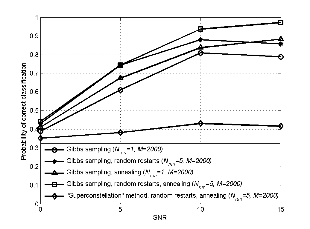
Figure 3: Probability of correct classification using Gibbs sampling versus SNR ($N=128$, $M_{t}=M_{r}=2$, $K=2$ and $L=5$).

V-A2 Performance Under Incorrect Channel Length Estimates

Next, we study the effect of incorrect channel length estimates. The relative powers of the considered channel taps are $[0\mathrm{\,dB},-2\mathrm{\,dB},-2.5\,\mathrm{dB}]$. We considered the performance of the proposed scheme under overestimated, correctly estimated, or underestimated channel lengths. Specifically, the channel length estimates take three possible values, namely $\hat{L}=1$, $\hat{L}=3$ or $\hat{L}=5$, while $L=3$. The same values for the parameters of Gibbs sampler are used as in Sec. V-A1. Fig. 4 shows the probabilities of correct classification for Gibbs sampling with both random restarts and annealing versus SNR. It is observed that there is a minor performance degradation with an overestimated channel length. Here, for this example, the degradation caused by the overfitting when a more complex model with $\hat{L}=5$ is used is minor. In contrast, a more severe performance degradation is observed for the case of the underestimated channel length. This significant degradation is caused by the bias introduced by the simpler model with $\hat{L}=1$. We also carried out the experiments for $L=5$ taps with relative powers of $[0\mathrm{\,dB},-2\mathrm{\,dB},-2.5\,\mathrm{dB},$ $-3.1\,\mathrm{dB,}$$-4.2\,\mathrm{dB}]$. The performance is very similar to that for the case of $L=3$ shown in Fig. 4 and is hence not reported here.

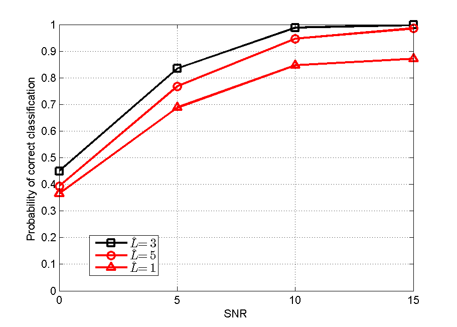
Figure 4: Probability of correct classification using Gibbs sampling versus SNR with different channel length estimates $\hat{L}$ ($N=128$, $M_{t}=M_{r}=2$, $K=2$ and $L=3$).

V-A3 Performance with a Larger $\mathcal{A}$

To study the effect of modulation pool $\mathcal{A}$ with a larger size, besides the three modulations considered above, we added 16-PSK into the modulation pool, i.e., $\mathcal{A}$={QPSK, 8-PSK, 16QAM, 16-PSK}. The relative powers of the multi-path components and the parameters of the Gibbs sampler take the same value as in Sec. V-A2. The performance of the proposed Gibbs sampler for the cases of three and four modulation formats is shown in Fig. 4. As expected, some performance degradation is observed for a larger set of possible modulation schemes. To gain more insight into the classifier behavior, the confusion matrices for both cases of three and four modulation schemes for SNR of 5 dB are shown in Tables II and III, respectively. The confusion matrices show the probabilities of deciding for a given modulation format when another format is the correct one. For instance, the element associated with row ‘8-PSK’ and column ‘QPSK’ in Table II indicates that, when the actual modulation scheme is 8-PSK, the probability that the estimated modulation is QPSK is 9.2%. Comparing Table II with Table III, it can be seen that the decreased accuracy is mainly caused by the confusion between the two most similar modulation formats, namely 8-PSK and 16-PSK.

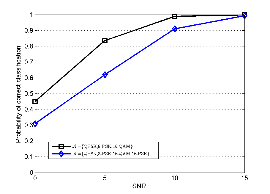
Figure 5: Probability of correct classification using Gibbs sampling versus SNR with different sets $\mathcal{A}$ of possible modulation schemes ($N=128$, $M_{t}=M_{r}=2$, $K=2$ and $L=3$).

Table II: Confusion matrix of the proposed Gibbs sampler for three modulation formats at 5 dB

		Estimated
		QPSK	8-PSK	16-QAM
Actual	QPSK	96.3%	2.7%	1.0%
	8-PSK	9.2%	88.1%	2.7%
	16-QAM	15.4%	18.6%	66.0%

Table III: Confusion matrix of the proposed Gibbs sampler for four modulation formats at 5 dB

		Estimated
		QPSK	8-PSK	16-QAM	16-PSK
Actual	QPSK	96.8%	1.8%	0.6%	0.8%
	8-PSK	9.4%	43.4%	3.6%	43.6%
	16-QAM	18.8%	11.6%	60.6%	9.0%
	16-PSK	11.8%	37.8%	3.8%	46.6%

V-B Performance of Mean Field Variational Inference

Here, we study the performance of a hybrid scheme, inspired by [39], that starts with a Gibbs sampler in order to perform a global search in the parameter space and then switches to mean field variational inference to speed up the convergence to a nearby local optima. In the switching iteration, all the needed marginal distributions for mean field variational inference are initialized as the conditional distributions for Gibbs sampling in the previous iteration, namely the marginal distributions are initialized as follows,

$$q^{(m_{s})}(\mathbf{p}_{A})=p^{(m_{s}-1)}(\mathbf{p}_{A}|\mathbf{s},\mathbf{h}\mathrm{,\sigma^{2}},\mathbf{y}),$$ (38)

$$q^{(m_{s})}(s_{m_{t}}[n,k])$$

$$= p^{(m_{s}-1)}(s_{m_{t}}[n,k]|\mathbf{p}_{A},\mathbf{s}\diagdown s_{m_{t}}[n,k],\mathbf{h\mathrm{,\sigma^{2},}}\mathbf{y}),$$ (39)

$$q^{(m_{s})}(\boldsymbol{\mathbf{h}}_{m_{t}m_{r}})$$

$$= p^{(m_{s}-1)}(\boldsymbol{\mathbf{h}}_{m_{t},m_{r}}|\mathbf{P}_{A},\mathbf{s},\mathbf{h}\diagdown\boldsymbol{\mathbf{h}}_{m_{t},m_{r}},\mathbf{\mathrm{\sigma^{2},}}\mathbf{y}),$$ (40)

and

$$q^{(m_{s})}(\sigma^{2})=p^{(m_{s}-1)}(\sigma^{2}|\mathbf{p}_{A}\mathbf{s},\mathbf{h},\mathbf{y}),$$ (41)

where $m_{s}$ denotes the index of the switching iteration.

To demonstrate the effectiveness of this approach, we consider modulation classification using received samples within one OFDM frame ($K=1$) over Rayleigh fading channels with two taps ($L=2$) and with the relative powers $[0\mathrm{\,dB},-4.2\,\mathrm{dB}]$. The SNR is $10\,\mathrm{dB}$ and the DFT size is $N=64$ or $128$. After the first eight iterations of regular Gibbs sampling (without random restarts and annealing), we switch to the mean field variational inference. The probability of correct classification of both regular Gibbs sampling and the hybrid approach versus the number of iterations $M$ with $M_{0}=0.9M$ burn-in samples is shown in Fig. 6. It can be observed that the hybrid approach outperforms Gibbs sampling especially when the number of iterations is small.

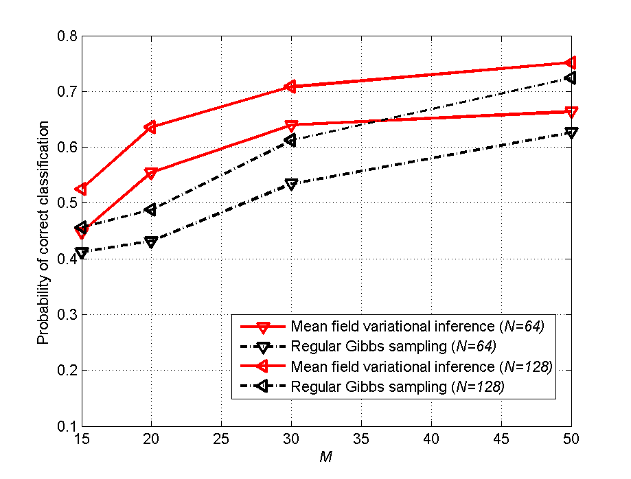
Figure 6: Probability of correct classification using Gibbs sampling and mean field variational inference versus $M$ ($M_{t}=M_{r}=2$, $K=1$, $L=2$ and SNR=$10\,\mathrm{dB}$).

V-C Comparison of Gibbs Sampling and ICA-PC [28]

Here, we compare the classification results achieved by the proposed Gibbs sampling scheme with the ICA-PC approach of [28], which extends to MIMO-OFDM the techniques studied in [22]. The approach in [28] exploits the invariance of the frequency-domain channels across the coherence bandwidth to perform classification. Specifically, the subcarriers are grouped in sets of $D$ adjacent subcarriers whose frequency-domain channel matrices are assumed to be identical. Let us denote the frequency-domain channel matrix and the received samples for the $i$-th group by $\mathbf{H}_{i}$ and $\mathbf{y}_{i}$ respectively, $i=1,...,N/D$. To compute the likelihood function $\,p(\mathbf{y}_{i}|A=a,\mathbf{H}_{i})$ of the received samples $\mathbf{y}_{i}$ over the subcarriers within group $i$, an estimate $\mathbf{\hat{H}}_{i}$ of the channel matrix $\mathbf{H}_{i}$ is first obtained using ICA-PC, and then the likelihood $p(\mathbf{y}_{i}|A=a,\mathbf{H}_{i})$ is approximated as $p(\mathbf{y}_{i}|A=a,\mathbf{\hat{H}}_{i})$. Accordingly, the likelihood function $p(\mathbf{y}|A=a,\mathbf{H})$ of all the received samples $\mathbf{y}$ is approximated as $p(\mathbf{y}|A=a,\mathbf{\hat{H}})=\prod_{i}p(\mathbf{y}_{i}|A=a,\mathbf{\hat{H}}_{i})$, where $\mathbf{\widehat{H}}=\{\mathbf{\hat{H}}_{i}\}_{i=1}^{N/D}$. The detected modulation is selected as $\widehat{A}=\arg\max_{a\in\mathcal{A}}p(\mathbf{y}|A=a,\mathbf{\hat{H}})$.

In Fig. 7, we plot the performance of the approach based on ICA-PC with different values of $D$ and Gibbs sampling with random restarts and annealing. The number of runs are $N_{run}=5$, and the annealing schedule is (26). It can be seen from Fig. 7 that Gibbs sampling significantly outperforms ICA-PC. In this regard, note that, with $D=4$, the accuracy in ICA-PC is poor due to the insufficient number of observed data samples; while with $D=16$, the model mismatch problem becomes more severe due to the assumption of equal channel matrices in each subcarrier group.

To further emphasize the advantages of the proposed Bayesian techniques, in Fig. 7, we consider the case in which there are fewer receive antennas than transmit antennas by setting $M_{r}=1$ and all other parameters as above. While ICA-PC cannot be applied due to the ill-posedness of the ICA problem, it can be observed that a success rate of $71\%$ can be attained by the proposed Gibbs scheme at $15\mathrm{\,dB}$. It should be mentioned however, that the complexity of ICA-PC of the order of $\mathcal{O}\{M_{t}M_{r}KNM_{u}^{M_{t}}\}$ [24] is smaller than that of Gibbs sampling (see Remark 5), where $M_{u}$ denotes the maximum number of states of a constellation among all the possible modulation types, i.e., $M_{u}=\max_{a\in\mathcal{A}}\{\left|a\right|\}$.

.

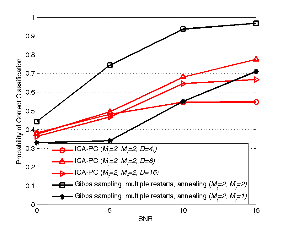
Figure 7: Probability of correct classification using Gibbs sampling with multiple random restarts and annealing and approach of [28] based on ICA-PC versus SNR ($N=128$, $K=2$ and $L=5$).

V-D Performance for Coded OFDM Signals

To investigate the performance of the proposed Gibbs sampling approach in the presence of a model mismatch, we study here the case of coded OFDM. Specifically, we assume that the information bits are first encoded using a convolutional code, and then modulated. We apply Gibbs sampling with multiple random restarts and annealing with all relevant parameters being the same as in Sec. V-A. The code rates are $1/3,$ $1/2$ and $2/3$, respectively. In Fig. 8, the probability of correct classification is shown versus SNR. It can be seen from the figure that the success rate decreases only slightly (up to 6%) as the code rate decreases. The degradation is caused by the fact that the coded transmitted symbols are not mutually independent due to the convolutional coding, and hence their prior distribution is mismatched with respect to the model (17). As the SNR increases, the performance degradation for coded signals become minor, because, in this regime, Gibbs sampling relies more on the observed samples than on the priors. We also studied the performance of the proposed Gibbs sampling for OFDM systems with space-frequency coded symbols (SF-OFDM) [48]. Compared to the uncoded case, minor performance degradation (2% at $15\mathrm{\,dB}$ and up to 8% at $0\mathrm{\,dB}$) is observed also due to the presence of a model mismatch.

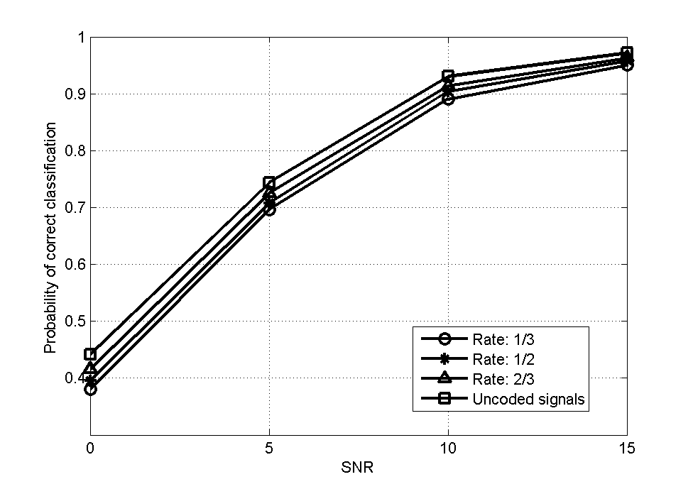
Figure 8: Probability of correct classification using Gibbs sampling with multiple random restarts and annealing versus SNR for convolution coded OFDM signals with different code rate ($N=128$, $M_{t}=M_{r}=2$, $K=2$ and $L=5$).

VI Conclusions

In this paper, we have proposed two Bayesian modulation classification schemes for MIMO-OFDM systems based on a selection of the prior distributions that adopts a latent Dirichlet model and on the Bayesian network formalism. The proposed Gibbs sampling method converges to an effective solution and, using numerical results, its accuracy is demonstrated to improve for small sample sizes when switching to the mean field variational inference technique after a number of iterations. The speed of convergence is shown to improve via multiple random restarts and annealing. The techniques are seen to overcome the performance limitation of state-of-the-art non-Bayesian schemes based on ICA and Bayesian schemes based on “superconstellation” methods. In fact, while most of the mentioned existing modulation classification algorithms rely on the assumptions that the channels are flat fading, that the number of receive antennas is no less than the number of transmit antenna, and/or that a large amount of samples are available (as for pattern recognition-based methods), the proposed schemes achieve satisfactory performance under more general conditions. For example, with $M_{t}=2$ transmit antennas and under frequency selective fading channels with $L=5$ taps, a correct classification rate of above $97\%$ may be attained with $M_{r}=2$ receive antennas and with 256 received samples at each antenna; and a success rate of above $70\%$ may be achieved with $M_{r}=1$ receive antenna and 256 received samples at the antenna. Moreover, the proposed Gibbs sampler presents a graceful degradation in the presence of a model mismatch caused by channel coding, e.g., a decrease in the success rate by $6\%$ with a code rate of $1/3$. Future works include devising a Gibbs sampling scheme that accounts for the effects of the timing and carrier frequency offsets for MIMO systems following, e.g., [21], [44], [49]. In addition, the development of Bayesian classification techniques that address non-Gaussian noise is also a topic for further investigation.

Appendix I

Distributions

In this Appendix, we give the expressions for all standard distributions that are useful to derive the conditional distributions for Gibbs sampling in Appendix II.

1. Dirichlet Distribution: $\mathbf{Z}\sim\mathrm{Dirichlet}\left(\mathbf{c}\right),$

   $$p\left(\mathbf{Z}\right)=\frac{\Gamma\left(\sum_{i=1}^{k_{z}}c_{i}\right)}{\prod_{i=1}^{k_{z}}\Gamma\left(c_{i}\right)}\prod_{i=1}^{k_{z}}z_{i}^{c_{i}-1},$$ (42)

   where $k_{z}$ denotes the length of the vector $\mathbf{Z}$, and $\Gamma(\cdot)$ stands for the gamma function [41].

2. Circular complex Gaussian distribution: $\mathbf{Z}\sim\mathcal{CN}(\mathbf{\mu},\mathbf{\Sigma})$,

   $$p\left(\mathbf{Z}\right)=\frac{1}{\pi^{k_{z}}\det\left(\mathbf{\Sigma}\right)}\exp\left\{-\left(\mathbf{Z}-\mathbf{\mu}\right)^{H}\mathbf{\Sigma}^{-1}\left(\mathbf{Z}-\mathbf{\mu}\right)\right\},$$ (43)

   where we use $\det(\cdot)$ to denote the determinant of a matrix.

3. Inverse Gamma distribution:: $z\sim\mathcal{IG}(c,d)$,

   $$p\left(\mathbf{Z}\right)=\frac{d^{c}}{\Gamma\left(c\right)}z^{-c-1}\exp\left(-\frac{d}{z}\right).$$ (44)

Appendix II

Derivations of Conditional Distributions for Gibbs Sampling

In this Appendix, the required conditional distributions for Gibbs sampling are derived.

A. Expression for $p(\mathbf{p}_{A}|\mathbf{s},\mathbf{h}\mathrm{,\sigma^{2}},\mathbf{y})$

Applying (10) to (17), we have

$$p\left(\mathbf{p}_{A}\Big{|}\mathbf{s},\mathbf{h}\mathrm{,\sigma^{2}},\mathbf{y}\right)$$

$$\propto p\left(\mathbf{p}_{A}\right)\bigg{\{}\prod_{n,k,m_{t}}p\left(s_{m_{t}}[n,k]|\mathbf{p}_{A}\right)\bigg{\}}$$

$$\propto \prod_{a\in\mathcal{A}}\left[\mathbf{p}_{A}\left(a\right)\right]^{\boldsymbol{\gamma}\left(a\right)-1}\prod_{n,k,m_{t}}\bigg{[}\sum_{a:\,s_{m_{t}}[n,k]\in a}\mathbf{p}_{A}\left(a\right)/\left|a\right|\bigg{]}$$

$$= \prod_{a\in\mathcal{A}}\frac{1}{\left|a\right|}\left[\mathbf{p}_{A}\left(a\right)\right]^{\boldsymbol{\gamma}\left(a\right)-1+c_{a}}$$

$$\sim \mathrm{Dirichlet}\left(\boldsymbol{\gamma}+\mathbf{c}\right),$$ (45)

where $\mathbf{c}=\left[c_{1},\cdots,c_{\left|\mathcal{A}\right|}\right]^{T}$, and $c_{a}$ is the number of samples of transmitted symbols in constellation $a\in\mathcal{A}$.

B. Expression for $p(\boldsymbol{\mathbf{h}}_{m_{t},m_{r}}|(\mathbf{P}_{A},\mathbf{s},\mathbf{h}\diagdown\boldsymbol{\mathbf{h}}_{m_{t},m_{r}},\mathbf{\mathrm{\sigma^{2},}}\mathbf{y}))$

Applying (10) to (17), we have

$$p\left(\boldsymbol{\mathbf{h}}_{m_{t},m_{r}}\Big{|}\left(\mathbf{P}_{A},\mathbf{s},\mathbf{h}\diagdown\boldsymbol{\mathbf{h}}_{m_{t},m_{r}},\mathbf{\mathrm{\sigma^{2},}}\mathbf{y}\right)\right)$$

$$\propto p\left(\boldsymbol{\mathbf{h}}_{m_{t},m_{r}}\right)p\left(\mathbf{y}\Big{|}\mathbf{p}_{A},\mathbf{s},\mathbf{h}\mathrm{,\sigma^{2}}\right)$$

$$\propto \exp\bigg{\{}-\boldsymbol{\mathbf{h}}_{m_{t},m_{r}}^{H}\left(\hat{\boldsymbol{\Sigma}}_{m_{t},m_{r}}\right)^{-1}\boldsymbol{\mathbf{h}}_{m_{t},m_{r}}+$$

$$2\mathrm{real}\left[\boldsymbol{\mathbf{h}}_{m_{t},m_{r}}^{H}\left(\hat{\boldsymbol{\Sigma}}_{m_{t},m_{r}}\right)^{-1}\hat{\mathbf{h}}_{m_{t},m_{r}}\boldsymbol{\mathbf{h}}_{m_{t},m_{r}}\right]\bigg{\}}$$

$$\sim \mathcal{CN}(\hat{\mathbf{h}}_{m_{t},m_{r}},\hat{\boldsymbol{\Sigma}}_{m_{t},m_{r}}),$$ (46)

where

$$\left(\hat{\boldsymbol{\Sigma}}_{m_{t},m_{r}}\right)^{-1} =\frac{1}{\alpha_{h}}\mathbf{I}+\frac{1}{\mathrm{\sigma^{2}}}\mathbf{W}^{H}\mathbf{D}_{m_{t}}^{H}\mathbf{D}_{m_{t}}\mathbf{W}$$

$$\approx\frac{1}{\mathrm{\sigma^{2}}}\mathbf{W}^{H}\mathbf{D}_{m_{t}}^{H}\mathbf{D}_{m_{t}}\mathbf{W},$$ (47)

and

$$\hat{\mathbf{h}}_{m_{t},m_{r}}= \hat{\boldsymbol{\Sigma}}_{m_{t},m_{r}}\frac{1}{\sigma^{2}}\mathbf{W}^{H}\mathbf{D}_{m_{t}}^{H}\cdot$$

$$\cdot\bigg{(}\mathbf{y}_{m_{r}}-\sum_{m_{t}^{\prime}\neq m_{t}}\mathbf{D}_{m_{t}^{\prime}}\tilde{\mathbf{h}}_{m_{t}^{\prime},m_{r}}\bigg{)},$$ (48)

where the approximation in (47) follows from the fact that $\alpha_{h}$ is very large such that the term $1/\alpha_{h}\mathbf{I}$ can be neglected.

C. Expression for $p\left(\sigma^{2}|\mathbf{p}_{A}\mathbf{s},\mathbf{h},\mathbf{y}\right)$

Applying (10) to (17), we have

$$p\left(\sigma^{2}\Big{|}\mathbf{p}_{A}\mathbf{s},\mathbf{h},\mathbf{y}\right)$$

$$\propto p\left(\sigma^{2}\right)p\left(\mathbf{y}\Big{|}\mathbf{p}_{A},\mathbf{s},\mathbf{h}\mathrm{,\sigma^{2}}\right)$$

$$\propto \left(\sigma^{2}\right)^{-\alpha_{0}-1}\exp\left(-\frac{\beta_{0}}{\sigma^{2}}\right)$$

$$\prod_{m_{r=1}}^{M_{r}}\frac{1}{\sigma^{2NK}}\exp\bigg{\{}-\frac{1}{\mathrm{\sigma^{2}}}\left\|\mathbf{y}_{m_{r}}-\sum_{m_{t=1}}^{M_{t}}\mathbf{D}_{m_{t}}\mathbf{\mathbf{W}}\mathbf{h}_{m_{t},m_{r}}\right\|^{2}\bigg{\}}$$

$$\propto \left(\mathrm{\sigma^{2}}\right)^{-(\alpha_{0}+M_{r}NK)-1}\cdot$$

$$\cdot\exp\bigg{(}-\frac{\beta_{0}+\sum_{m_{r=1}}^{M_{r}}\left\|\mathbf{y}_{m_{r}}-\sum_{m_{t=1}}^{M_{t}}\mathbf{D}_{m_{t}}\mathbf{\mathbf{W}}\mathbf{h}_{m_{t},m_{r}}\right\|^{2}}{\sigma^{2}}\bigg{)}$$

$$\sim \mathcal{IG}\left(\alpha,\beta\right),$$ (49)

where $\alpha=\alpha_{0}+NKM_{r}$ and $\beta=\beta_{0}+\sum_{m_{r}}\left\|\mathbf{\mathbf{y}}_{m_{r}}-\sum_{m_{t}}\mathbf{D}_{m_{t}}\tilde{\mathbf{h}}_{m_{t},m_{r}}\right\|^{2}$.

Appendix III

Evaluation of (29)

By taking expectation with respect to updated distribution $q\left(\mathbf{\mathbf{\mathbf{p}_{A}}}\right)$ and $q\left(\mathbf{s}[n,k]\diagdown s_{m_{t}}[n,k],\mathbf{h},\sigma^{2}\right)$ receptively, it can be shown that the expression for $\big{\langle}\ln p\left(s_{m_{t}}[n,k]|\mathbf{p}_{A}\right)\big{\rangle}_{\mathbf{p}_{A}}$ is

$$\big{\langle}\ln p\left(s_{m_{t}}[n,k]|\mathbf{p}_{A}\right)\big{\rangle}_{q\left(\mathbf{\mathbf{\mathbf{p}_{A}}}\right)}$$

$$= \sum_{a\in\mathcal{A}}\mathrm{\mathbf{1}}\left(s_{m_{t}}[n,k]\in a\right)\left[\psi\left(\gamma_{a}\right)-\psi\left(\gamma_{0}\right)-\ln\left|a\right|\right],$$ (50)

where $\gamma_{0}=\sum_{a\in\mathcal{A}}\gamma_{a}$; and the expression for $\big{\langle}\ln p\left(\mathbf{y}[n,k]|\mathbf{s}[n,k],\mathbf{H}[n],\sigma^{2}\right)\big{\rangle}$ is

$$\big{\langle}\ln p\left(\mathbf{y}[n,k]|\mathbf{s}[n,k],\mathbf{H}[n],\sigma^{2}\right)\big{\rangle}_{q\left(\mathbf{s}[n,k]\diagdown s_{m_{t}}[n,k],\mathbf{h},\sigma^{2}\right)}$$

$$\propto \frac{\alpha}{\beta}\bigg{\{}2\mathrm{real}\left[\mathbf{y}^{H}[n,k]\right]\big{\langle}\mathbf{H}[n]\big{\rangle}\big{\langle}\mathbf{s}[n,k]\big{\rangle}_{q\left(\mathbf{s}[n,k]\diagdown s_{m_{t}}[n,k]\right)}$$

$$-\mathrm{tr}\left(\big{\langle}\mathbf{H}^{H}[n]\mathbf{H}[n]\big{\rangle}\mathrm{cov\left(\mathbf{s}[n,k]\right)}\right)$$

$$-\big{\langle}\mathbf{s}[n,k]\big{\rangle}_{q\left(\mathbf{s}[n,k]\diagdown s_{m_{t}}[n,k]\right)}^{H}\cdot$$

$$\cdot\big{\langle}\mathbf{H}^{H}[n]\mathbf{H}[n]\big{\rangle}\big{\langle}\mathbf{s}[n,k]\big{\rangle}_{q\left(\mathbf{s}[n,k]\diagdown s_{m_{t}}[n,k]\right)}\bigg{\}},$$ (51)

with the $(m_{t}^{\prime},m_{t}^{\prime\prime})$ element of the covariance matrix of the vector $\mathbf{s}[n,k]$

$$\mathrm{cov}\left(\mathbf{s}[n,k]\right)_{(m_{t}^{\prime},m_{t}^{\prime\prime})}$$

$$= \mathrm{var(}s_{m_{t}^{\prime}}[n,k])$$

$$= \begin{cases}\big{\langle}\left|s_{m_{t}^{\prime}}[n,k]\right|^{2}\big{\rangle}-\big{\langle}\left|s_{m_{t}^{\prime}}[n,k]\right|\big{\rangle}^{2},&\mathrm{if}\>m_{t}^{\prime}=m_{t}^{\prime\prime},\\ &m_{t}^{\prime\prime}\neq m_{t};\\ 0,&\mathrm{otherwise}.\end{cases}$$ (52)

the $m_{t}^{\prime}$-th element of $\big{\langle}\mathbf{s}[n,k]\big{\rangle}_{q\left(\mathbf{s}[n,k]\diagdown s_{m_{t}}[n,k]\right)}$ being

$$\big{\langle}\mathbf{s}[n,k]\big{\rangle}_{(m_{t}^{,})} =\begin{cases}\big{\langle}s_{m_{t}^{\prime}}[n,k]\big{\rangle},&\mathrm{if\>}m_{t}^{\prime}\neq m_{t}\\ s_{m_{t}}[n,k],&\mathrm{if}\>m_{t}^{\prime}=m_{t}\end{cases},$$ (53)

the $(m_{r}^{\prime},m_{t}^{\prime})$ element of $\big{\langle}\mathbf{H}[n]\big{\rangle}$ being the $n$-th element of the matrix product $\mathbf{W\mathbf{\widehat{h}}_{m_{t}^{\prime},m_{r}^{\prime}}}$, and the $(m_{t}^{\prime},m_{t}^{\prime\prime})$ element of $\big{\langle}\mathbf{H}^{H}[n]\mathbf{H}[n]\big{\rangle}$ being

$$\left[\big{\langle}\mathbf{H}^{H}[n]\mathbf{H}[n]\big{\rangle}\right]_{\left(m_{t}^{\prime},m_{t}^{\prime\prime}\right)}=$$

$$\begin{cases}\sum_{m_{r}=1}^{M_{r}}\Bigg{\{}\mathrm{tr}\left[\left[\mathbf{W}_{(n,\cdot)}\right]^{H}\mathbf{W}_{(n,\cdot)}\mathbf{\boldsymbol{\Sigma}}_{m_{t}^{\prime\prime},m_{r}}\right]+\\ \big{\langle}\mathbf{h}_{m_{t}^{\prime\prime},m_{r}}\big{\rangle}^{H}\left[\mathbf{W}_{(n,\cdot)}\right]^{H}\mathbf{W}_{(n,\cdot)}\big{\langle}\mathbf{h}_{m_{t}^{\prime\prime},m_{r}}\big{\rangle}\Bigg{\}},&\mathrm{if\>}m_{t}^{\prime}=m_{t}^{\prime\prime};\\ \big{\langle}\mathbf{H}[n]\big{\rangle}_{\left(\cdot,m_{t}^{\prime}\right)}\big{\langle}\mathbf{H}[n]\big{\rangle}_{\left(\cdot,m_{t}^{\prime\prime}\right)},&\mathrm{if}\>m_{t}^{\prime}\neq m_{t}^{\prime\prime}.\end{cases}$$ (54)

References

• [1] J. Mitola, “Cognitive radio for flexible mobile multimedia communications,” in Proceeding IEEE International Workshop on mobile and multimedia communications, San Diego, CA, USA, Nov. 1999.
• [2] O. A. Dobre, S. Rajan and R. Inkol, “Joint signal detection and classification based on first-order cyclostationarity for cognitive radios,” EURASIP J. Adv. Signal Process., vol. 2009, no. 1, p. 656719, Sep. 2009.
• [3] O. A. Dobre, A. Abdi, Y. Bar-Ness and W. Su, “A survey of automatic modulation classification techniques: classical approaches and new developments,” IET Communications, vol.1, no. 2, pp. 137-156, Apr. 2007.
• [4] A. Gelman, J. B. Carlin, H. S. Stern, D. B. Dunson, A. Vehtari and D. B. Rubin, Bayesian Data Analysis, CRC Press, 2013.
• [5] F. Hameed, O. A. Dobre, and D. C. Popescu, “On the likelihood-based approach to modulation classification,” IEEE Transactions on Wireless Communications, vol. 8, no. 12, pp. 5884 - 5892, Dec. 2009.
• [6] J. L. Xu, W. Su, and M. Zhou, “Software-defined radio equipped with rapid modulation recognition,” IEEE Trans. Veh. Technol., vol. 59, no. 4, pp. 1659-1667, May 2010.
• [7] O. A. Dobre, A. Abdi, Y. Bar-Ness, and W. Su, “Blind modulation classification: a concept whose time has come," in Proc. IEEE Sarnoff Symposium , pp. 223-228, Princeton, NJ, April 2005.
• [8] O. A. Dobre and F. Hameed, “Likelihood-based algorithms for linear digital modulation classification in fading channels,” in Proc. 19th IEEE Canadian Conf. Electrical Computer Engineering, pp. 1347-1350, Ottawa, Ontario, Canada, May 2006.
• [9] C. Y. Huang and A. Polydoros, “Likelihood methods for MPSK modulation classification,” IEEE Trans. Commun., vol. 43, no. 2/3/4, pp. 1493-1504, 1995.
• [10] C. Long, K. Chugg, and A. Polydoros, “Further results in likelihood classification of QAM signals,” in Proc. IEEE MILCOM, pp. 57-61, Fort Monmouth, NJ, Oct. 1994.
• [11] W. Wei and J. Mendel, “Maximum-likelihood classification for digital amplitude-phase modulations,” IEEE Trans. Commun., vol. 48, no. 2, pp. 189-193, Feb. 2000.
• [12] A. Abdi, O. A. Dobre, R. Choudhry, Y. Bar-Ness, and W. Su, “Modulation classification in fading channels using antenna arrays,” in Proc. IEEE MILCOM, pp. 211-217, 2004.
• [13] O. A. Dobre, J. Zarzoso, Y. Bar-Ness, and W. Su, “On the classification of linearly modulated signals in fading channels," in Proc. Conf. Inform. Sciences Systems (CISS), Princeton, NJ, 2004.
• [14] Hong, Liang, and Ho, K.C, “BPSK and QPSK modulation classification with unknown signal level,” in Proc. IEEE MILCOM, no.2, pp. 976–980, Los Angeles, CA, 2000.
• [15] O. A. Dobre, Y. Bar-Ness, and W. Su, “Robust QAM modulation classification algorithm based on cyclic cumulants,” in Proc. WCNC, 2004, pp. 745-748, 2004.
• [16] O. A. Dobre, Y. Bar-Ness, and W. Su, “Higher-order cyclic cumulants for high order modulation classification,” in Proc. MILCOM, pp. 112-117, 2003.
• [17] C. M. Spooner, “On the utility of sixth-order cyclic cumulants for RF signal classification,” in Proc. ASILOMAR, pp. 890-897, Pacific Grove, CA, Nov. 2001.
• [18] [44] K. C. Ho, W. Prokopiw, and Y. T. Chan, “Modulation identification of digital signals by the wavelet transform,” In Proc. Radar, Sonar and Navig., vol. 47, pp. 169-176, 2000.
• [19] T. A. Drumright and Z. Ding. “QAM constellation classication based on statistical sampling for linear distortive channels,” IEEE Trans. Signal Process., vol. 54, no. 5, pp. 1575-1586, May 2006.
• [20] Y. Liu, O. Simeone, A. Haimovich and W. Su, “Modulation classification via Gibbs sampling based on a latent Dirichlet Bayesian network,” IEEE Signal Proc. Letters, vol. 21, no. 9, pp. 1135-1139, Sep. 2014.
• [21] S. Amuru and C. R. C. M. Da Silva, “A blind preprocessor for modulation classification applications in frequency-selective non-Gaussian channels”, IEEE Trans. Communications, vol. 63, no. 1, pp. 156-169, Jan. 2015.
• [22] V. Choqueuse, S. Azou, K. Yao, L. Collin and G. Burel, “Blind Modulation recognition for MIMO Systems,” MTA Review, vol. XIX, no. 2, pp. 183-195, June 2009.
• [23] M. S. Muhlhaus, M. Oner, O. A. Dobre, H. U. Jakel and F. K. Jondral, “Automatic modulation classification for MIMO systems using forth-order cumulatns,” in Proc. IEEE Vehic. Technology Conf. Fall, pp. 1-5, Quebec City, QC, CAN., Sep. 2012.
• [24] M. S. Muhlhaus, M. Oner, O. A. Dobre and F. K. Jondral, “A low complexity modulation classification algorithm for MIMO systems,” IEEE Communications Letters, vol. 17, no. 10, pp. 1881-1884, Oct. 2013.
• [25] K. Hassan, I. Dayoub, W. Hamouda, C. N. Nzeza and M. Berineau, “Blind digital modulation identification for spatially-correlated MIMO systems,” IEEE trans. Wireless Commun., vol. 11, no. 2, pp. 683-693, Feb. 2012.
• [26] M. Marey and O. A. Dobre, “Blind modulation classification algorithm for single and multiple-antenna systems over frequency-selective channels,” IEEE Signal Proc. Letters, vol. 21, no. 9, pp. 1098-1102, Sep. 2014.
• [27] A. Hyvarinen, J. Karhunen and E. Oja, Independent Component Analysis, Wiley-Interscience, 2001.
• [28] A. Agirman-Tosun, Y. Liu, A. M. Haimovich, O. Simeone, W. Su, j. Dabin and E. kanterakis, “Modulation classification of MIMO-OFDM signals by independent component analysis and support vector machines,” IEEE Asilomar Conference, CA, Nov. 2011.
• [29] Y. Liu, O. Simeone, A. Haimovich and W. Su, “Modulation classification of MIMO-OFDM signals by Gibbs sampling,” in Proc. the 49th Conference on Information Sciences and Systems (CISS), no. 1, pp. 1-6, Baltimore, MA. Mar. 18-20, 2015.
• [30] D. Blei, A. Ng, and M. Jordan, “Latent Dirichlet allocation,” Journal of Machine Learning Research, vol. 3, no. 1, pp. 993–1022, Jan. 2003.
• [31] S. kirkpatrick, C. D. Gelatt and M. P. Vecchi, “ Optimization by simulated annealing,” Science, vol. 220, no. 4598, pp. 671-680, May 1983.
• [32] Y. Nourani and B. Andresen, “A comparison of simulated annealing cooling strategies,” J. Phys. A, vol. 31, no. 41, pp. 8373-8385, July 1998.
• [33] C. Fevotte and S. J. Godsill, “A Bayesian approach for blind separation of sparse sources,” IEEE Trans. Audio, Speech and Language Process., vol. 14, no. 6, pp. 2174-2188, Nov. 2006.
• [34] A. , B. Sundar Rajan, Large MIMO Systems, Cambridge University Press, Feb. 2014.
• [35] C. P. Robert and G. Casella, Monte Carlo Statistical Methods, Springer, 1999.
• [36] R. M. Neal, “Sampling from multimodal distributions using tempered transitions,” Statistics and computing, vol. 6, no. 4, pp. 353-366, June 1996.
• [37] Y. Wang and K. Cheng, “A two-Stage Bayesian network method for 3D human pose estimation from monocular image sequences,” EURASIP J. Adv. Signal Process., vol. 2010, no. 1, p. 761460, April 2010.
• [38] D. Koller and N. Friedman, Probabilistic Graphical Models: Principles and Techniques, MIT Press, 2009.
• [39] A. T. Cemgil, F. Cedric and S. J. Godsill, “Variational and stochastic inference for Bayesian source separation,” Digital Signal Processing, vol. 17, pp. 891-913, Feb. 2007.
• [40] D. M. Blei and M. I. Jordan, “Variational inference for Dirichlet process mixtures,” Bayesian Analysis, vol. 1, no. 1, pp. 121-144, July 2006.
• [41] M. Abramowitz and I. Stegun, Handbook of Mathematical Functions: with Formulas, Graphs, and Mathematical Tables, Dover Publications, June 1972.
• [42] S. Aouda, A M. Zoubir, C. M. S. See, “A comparative study on source number detection”, in Proc. International Symposium on Signal Processing and Its Applications, vol. 1, pp. 173-176, Paris, France, Jul. 2003.
• [43] O. Somekh, O. Simeone, Y. Bar-Ness and Wei Su, “’Detecting the number of transmit antennas with unauthorized or cognitive receivers in MIMO systems,” in Proc. IEEE MILCOM, Orlando, FL, USA, Oct. 2007.
• [44] F. Z. Merli, X. Wang, G. M. Vitetta, “A Bayesian multiuser detection algorithm for MIMO-OFDM systems affected by multipath fading, carrier frequency offset, and phase noise,” IEEE J. ON Selected. Areas in Commun., vol. 26, no. 3, pp. 506- 516, April 2008.
• [45] K. P. Murphy, “Conjugate Bayesian analysis of the Gaussian distribution,” Univ. of British Columbia, Canada, Tech. Rep., 2007 [Online]. Available: http://www.cs.ubc.ca/~murphyk/Papers/bayesGauss.pdf
• [46] Z. Ghahramani and M. Beal, “Propagation algorithms for variational Bayesian learning, Neural Inform,” Advances in Neural Information Processing Systems, vol. 13, no.1 pp. 507-513, 2001.
• [47] A. B. Cote and M. I. Jordan, “Optimization of structured mean field objectives,” in Proc. The Twenty-Fifth Conference on Uncertainty in Artificial Intelligence, no.1, pp. 67-74, 2009.
• [48] K. F. Lee and D. B. Willims, “A space-frequency transmitter diversity technique for OFDM systems,” in Proc. GLOBECOM, vol. 3, pp. 1473-1477, Nov. 2000.
• [49] B. Lu, X. Wang, “Bayesian blind turbo receiver for coded OFDM systems with frequency offset and frequency-selective fading”, IEEE J. Selected. Areas in Commun., vol. 19, no. 12, pp. 2516-2527, Dec. 2001.