GPS-Denied Relative Motion Estimation For Fixed-Wing UAV Using the Variational Pose Estimator

Abstract

Relative pose estimation between fixed-wing unmanned aerial vehicles (UAVs) is treated using a stable and robust estimation scheme. The motivating application of this scheme is that of “handoff” of an object being tracked from one fixed-wing UAV to another in a team of UAVs, using onboard sensors in a GPS-denied environment. This estimation scheme uses optical measurements from cameras onboard a vehicle, to estimate both the relative pose and relative velocities of another vehicle or target object. It is obtained by applying the Lagrange-d’Alembert principle to a Lagrangian constructed from measurement residuals using only the optical measurements. This nonlinear pose estimation scheme is discretized for computer implementation using the discrete Lagrange-d’Alembert principle, with a discrete-time linear filter for obtaining relative velocity estimates from optical measurements. Computer simulations depict the stability and robustness of this estimator to noisy measurements and uncertainties in initial relative pose and velocities.

1 INTRODUCTION

Onboard estimation of relative motion between unmanned vehicles and spacecraft is an important enabling technology for autonomous operations of teams and formations of such vehicles. A stable relative motion estimation scheme that is robust to measurement noise and requires no knowledge of the dynamics model of the vehicle being observed, is presented here. This estimation scheme can enhance the autonomy and reliability of teams of unmanned vehicles operating in uncertain GPS-denied environments. Salient features of this estimation scheme are: (1) use of only onboard optical sensors for estimation of relative pose and velocities; (2) robustness to uncertainties and lack of knowledge of dynamics model of observed vehicle; (3) low computational complexity such that it can be implemented with onboard processors; and (4) proven stability with large domain of attraction for relative motion state estimation errors. Stable and robust relative motion estimation of unconstrained motion of teams of unmanned vehicles in the absence of complete knowledge of their dynamics, is required for their safe, reliable, and autonomous operations in poorly known environments. In practice, the dynamics of an observed vehicle may not be perfectly known, especially in outdoor environments where the vehicle may be under the action of unknown forces and moments. The scheme proposed here has a single, stable algorithm for the naturally coupled relative translational and rotational motion between unmanned vehicles, using measurements from onboard optical sensors. This avoids the need for measurements from external sources, like GPS, which may not be available in indoor, underwater or cluttered environments [2, 16, 21].

Relative pose (position and attitude) estimation of one vehicle from another vehicle is treated here. Determining the relative attitude requires that at least three feature points on the observed vehicle are available. Attitude estimation and control schemes that use generalized coordinates or quaternions for attitude representation are usually unstable in the sense of Lyapunov, as has been shown in recent research [3, 5, 25]. One adverse consequence of these unstable estimation and control schemes is that they end up taking longer to converge compared to stable schemes with the same initial conditions and same initial transient behavior. Attitude observers and filtering schemes on $\mathrm{SO(3)}$ and $\mathrm{SE(3)}$ have been reported in, e.g., [4, 14, 15, 17, 18, 19, 24, 27, 31, 32]. These estimators do not suffer from kinematic singularities like estimators using coordinate descriptions of attitude, and they do not suffer from the unstable unwinding phenomenon encountered by continuous estimators using unit quaternions. Recently, the maximum-likelihood (minimum energy) filtering method of Mortensen [23] was applied to attitude and pose estimation on $\mathrm{SO(3)}$ and $\mathrm{SE(3)}$, resulting in nonlinear estimation schemes that seek to minimize the stored “energy” in measurement errors [1, 34, 35]. This led to “near optimal” filtering schemes that are based on approximate solutions of the Hamilton-Jacobi-Bellman (HJB) equation and do not have provable stability. The estimation scheme obtained here is shown to be almost globally asymptotically stable. Moreover, unlike filters based on Kalman filtering, the estimator proposed here does not make any assumptions on the statistics of initial state estimate or sensor noise.

For the relative pose estimation problem analyzed in this paper, it is assumed that one vehicle can optically measure a known pattern fixed to the body of another vehicle whose relative motion states are to be estimated. From such optical (camera) measurements, the relative velocities (translational and angular) are also estimated. The variational attitude estimator recently appeared [10, 11], where it was shown to be almost globally asymptotically stable. The advantages of this scheme over Kalman-based schemes are reported in [9]. A companion paper extends the variational attitude estimator to estimation of coupled rotational (attitude) and translational motion. Maneuvering vehicles, like UAVs tracking ground targets, have naturally coupled rotational and translational motion. In such applications, designing separate state estimators for the translational and rotational motions may not be effective and could lead to poor navigation. For relative pose estimation between such vehicles operating in teams, the approach proposed here for robust and stable estimation will be more effective than Kalman filtering-based schemes. The estimation scheme proposed here can be implemented without any velocity measurements, which is useful when Doppler lidar sensors are not available onboard or rate gyros are corrupted by high noise content and bias [6, 7, 8].

2 RELATIVE NAVIGATION USING OPTICAL SENSORS

2-A Motivation

When multiple UAV perform surveillance and target tracking missions in a GPS-denied environment, they need to ensure that they are tracking the same target of interest. When necessary, the tracking responsibility may need to be handed off from one UAV to another. When GPS signals are available, such a handoff procedure can be achieved by a tracking UAV geo-locating the target and sending the global coordinates of the target to a handoff UAV. In GPS-denied environments, such a handoff procedure faces several challenges. The most significant challenge is the following: because no GPS signals are available, the handoff UAV may not know the position of the tracking UAV. Therefore, it needs to use on-board sensors to detect and navigate towards the tracking UAV. Moreover, global information about the target is not available. Because the tracking UAV does not have GPS, it can only geo-locate the target in its own navigation frame. Since the handoff UAV has a different coordinate system than the tracking UAV, the target information from the tracking UAV cannot be directly used by the handoff UAV to track the target. The handoff UAV has to perform a coordinate transformation that converts the target information to its own navigation frame. This task is carried out by the relative pose estimation technique presented here.

2-B Relative Pose Measurement Model

Let $O$ denote the observed vehicle and $S$ denote the vehicle that is observing $O$. Let $\mathsf{S}$ denote a coordinate frame fixed to $S$ and $\mathsf{O}$ be a coordinate frame fixed to $O$. Let $R\in\mathrm{SO(3)}$ be the rotation matrix from frame $\mathsf{S}$ to frame $\mathsf{O}$ and $b$ denote the position of origin of $\mathsf{S}$ expressed in frame $\mathsf{O}$. The pose (transformation) of frame $\mathsf{S}$ to frame $\mathsf{O}$ is

$$\mathsf{g}=\begin{bmatrix}R&b\\ 0&1\end{bmatrix}\in\mathrm{SE(3)}.$$ (1)

The positions of a fixed set of feature points or patterns on vehicle $O$ are observed by optical sensors fixed to vehicle $S$. Velocities of these points are not directly measured, but may be calculated using a simple linear filter as in [10]. Assume that there are $\mathpzc j>2$ feature points, which are always in the sensor field-of-view (FOV) of the sensor fixed to vehicle $S$, and the positions of these points are known in frame $\mathsf{O}$ as $p_{j}$, $j\in\{1,2,\ldots,\mathpzc j\}$. These points generate ${\mathpzc j\choose 2}$ unique pairwise relative position vectors, which are the vectors connecting any two of these points.

Denote the position of the optical sensor on vehicle $S$ and the vector from that sensor to an observed point on vehicle $O$ as $s\in\mathbb{R}^{3}$ and $q_{j}\in\mathbb{S}^{2}$, $j=1,2,\ldots,\mathpzc j$, respectively, both vectors expressed in frame $\mathsf{S}$. Thus, in the absence of measurement noise

$$p_{j}=R(q_{j}+s)+b=Ra_{j}+b,\;j\in\{1,2,\ldots,\mathpzc j\},$$ (2)

where $a_{j}=q_{j}+s$, are positions of these points expressed in $\mathsf{S}$. In practice, the $a_{j}$ are obtained from proximity optical measurements that will have additive noise; denote by $a_{j}^{m}$ the measured vectors. The mean values of the vectors $p_{j}$ and $a_{j}^{m}$ are denoted as $\bar{p}$ and $\bar{a}^{m}$, and satisfy

$$\bar{a}^{m}=R^{\mbox{\small T}}(\bar{p}-b)+\bar{\varsigma},$$ (3)

where $\bar{p}=\frac{1}{\mathpzc j}\sum\limits j_{j=1}p_{j}$, $\bar{a}^{m}=\frac{1}{\mathpzc j}\sum\limits j_{j=1}a_{j}^{m}$ and $\bar{\varsigma}$ is the additive measurement noise obtained by averaging the measurement noise vectors for each of the $a_{j}$. Consider the ${\mathpzc j\choose 2}$ relative position vectors from optical measurements, denoted as $d_{j}=p_{\lambda}-p_{\ell}$ in frame $\mathsf{O}$ and the corresponding vectors in frame $\mathsf{S}$ as $l_{j}=a_{\lambda}-a_{\ell}$, for $\lambda,\ell\in\{1,2,\ldots,\mathpzc j\}$, $\lambda\neq\ell$. Therefore,

$$d_{j}=Rl_{j}\Rightarrow D=RL,$$ (4)

where $D=[d_{1}\;\,\cdots\;\,d_{\beta}]$, $L=[l_{1}\;\,\cdots\;\,l_{\beta}]\in\mathbb{R}^{3\times\beta}$ with $\beta={\mathpzc j\choose 2}$. Note that the matrix of known relative vectors $D$ is assumed to be known and bounded. Denote the measured value of matrix $L$ in the presence of measurement noise as $L^{m}$. Then,

$$L^{m}=R^{\mbox{\small T}}D+\mathscr{L},$$ (5)

where $\mathscr{L}\in\mathbb{R}^{3\times\beta}$ is the matrix of measurement errors in these vectors observed in frame $\mathsf{S}$.

2-C Relative Velocities Measurement Model

Denote the relative angular and translational velocity of vehicle $O$ expressed in frame $\mathsf{S}$ by $\Omega$ and $\nu$, respectively. Thus, one can write the kinematics of the rigid body as

$$\dot{\Omega}=R\Omega^{\times},\dot{b}=R\nu\Rightarrow\dot{\mathsf{g}}=\mathsf{g}\xi^{\vee},$$ (6)

where $\xi=\begin{bmatrix}\Omega\\ \nu\end{bmatrix}\in\mathbb{R}^{6}$ and $\xi^{\vee}=\begin{bmatrix}\Omega^{\times}&\;\nu\\ 0\;\;&0\end{bmatrix}$ and $(\cdot)^{\times}:\mathbb{R}^{3}\to\mathfrak{so}(3)\subset\mathbb{R}^{3\times 3}$ is the skew-symmetric cross-product operator that gives the vector space isomorphism between $\mathbb{R}^{3}$ and $\mathfrak{so}(3)$. In order to do so, one can differentiate (2) as follows

$$\dot{p}_{j}=R\Omega^{\times}a_{j}+R\dot{a}_{j}+\dot{b}=R\big{(}\Omega^{\times}a_{j}+\dot{a}_{j}+\nu\big{)}=0$$

$$\Rightarrow \dot{a}_{j}-a_{j}^{\times}\Omega+\nu=0$$

$$\Rightarrow v_{j}=\dot{a}_{j}=[a_{j}^{\times}\;-I]\xi=G(a_{j})\xi,$$ (7)

where $G(a_{j})=[a_{j}^{\times}\;-I]$ has full row rank. From vision-based or Doppler lidar sensors, one can also measure the velocities of the observed points in frame $\mathsf{S}$, denoted $v_{i}^{m}$. Here, velocity measurements as would be obtained from vision-based sensors is considered. The measurement model for the velocity is of the form

$$v_{j}^{m}=G(a_{j})\xi+\vartheta_{j},$$ (8)

where $\vartheta_{j}\in\mathbb{R}^{3}$ is the additive error in velocity measurement $v_{j}^{m}$. Instantaneous angular and translational velocity determination from such measurements is treated in [26]. Note that $v_{j}=\dot{a}_{j}$, for $j\in\{1,2,\ldots,\mathpzc j\}$. As this kinematics indicates, the relative velocities of at least three beacons are needed to determine the vehicle’s translational and angular velocities uniquely at each instant. The rigid body velocities are obtained using the pseudo-inverse of $\mathds{G}(A^{f})$:

$$\mathds{G}(A^{f})\xi^{f} =\mathds{V}(V^{f})\Rightarrow\xi^{f}=\mathds{G}^{\ddagger}(A^{f})\mathds{V}(V^{f}),$$ (9)

$$\mbox{where }\;\mathds{G}(A^{f}) =\begin{bmatrix}G(a^{f}_{1})\\ \vdots\\ G(a^{f}j)\end{bmatrix}\;\mbox{and }\;\mathds{V}(V^{f})=\begin{bmatrix}v^{f}_{1}\\ \vdots\\ v^{f}j\end{bmatrix}.$$ (10)

When at least three beacons are measured, $\mathds{G}(A^{f})$ is a full column rank matrix, and $\mathds{G}^{\ddagger}(A^{f})=\Big{(}\mathds{G}^{\mbox{\small T}}(A^{f})\mathds{G}(A^{f})\Big{)}^{-1}\mathds{G}^{\mbox{\small T}}(A^{f})$ gives its pseudo-inverse. For the case that only one or two beacons are observed, $\mathds{G}(A^{f})$ is a full row rank matrix, whose pseudo-inverse is given by $\mathds{G}^{\ddagger}(A^{f})=\mathds{G}^{\mbox{\small T}}(A^{f})\Big{(}\mathds{G}(A^{f})\mathds{G}^{\mbox{\small T}}(A^{f})\Big{)}^{-1}$.

3 DYNAMIC ESTIMATION OF MOTION FROM PROXIMITY MEASUREMENTS

In order to obtain state estimation schemes from measurements as outlined in Section 2 in continuous time, the Lagrange-d’Alembert principle is applied to an action functional of a Lagrangian of the state estimate errors, with a dissipation term linear in the velocities estimate error. This section presents the estimation scheme obtained using this approach. Denote the estimated pose and its kinematics as

$$\hat{\mathsf{g}}=\begin{bmatrix}\hat{R}&\;\;\;\hat{b}\\ 0&\;\;\;1\end{bmatrix}\in\mathrm{SE(3)},\;\;\dot{\hat{\mathsf{g}}}=\hat{\mathsf{g}}\hat{\xi}^{\vee},$$ (11)

where $\hat{\xi}$ is rigid body velocities estimate, with $\hat{\mathsf{g}}_{0}$ as the initial pose estimate and the pose estimation error as

$$\mathsf{h}=\mathsf{g}\hat{\mathsf{g}}^{-1}=\begin{bmatrix}Q&\;\;\;\;b-Q\hat{b}\\ 0&\;\;1\end{bmatrix}=\begin{bmatrix}Q&\;\;\;x\\ 0&\;\;\;1\end{bmatrix}\in\mathrm{SE(3)},$$ (12)

where $Q=R\hat{R}^{\mbox{\small T}}$ is the attitude estimation error and $x=b-Q\hat{b}$. Then one obtains, in the case of perfect measurements,

$$\begin{split}&\dot{\mathsf{h}}=\mathsf{h}\varphi^{\vee},\,\mbox{ where }\,\varphi(\hat{\mathsf{g}},\xi^{m},\hat{\xi})=\begin{bmatrix}\omega\\ \upsilon\end{bmatrix}={\mathrm{Ad}_{\hat{\mathsf{g}}}}\big{(}\xi^{m}-\hat{\xi}),\end{split}$$ (13)

where ${\mathrm{Ad}_{\mathpzc{g}}}=\begin{bmatrix}\mathpzc{R}~{}&~{}0\\ \mathpzc{b}^{\times}\mathpzc{R}~{}&~{}\mathpzc{R}\end{bmatrix}$ for $\mathpzc{g}=\begin{bmatrix}\mathpzc{R}&\;\;\mathpzc{b}\\ 0&\;\;1\end{bmatrix}$. The attitude and position estimation error dynamics are also in the form

$$\dot{Q}=Q\omega^{\times},\;\;\dot{x}=Q\upsilon.$$ (14)

3-A Lagrangian from Measurement Residuals

Consider the sum of rotational and translational measurement residuals between the measurements and estimated pose as a potential energy-like function. Defining the trace inner product on $\mathbb{R}^{n_{1}\times n_{2}}$ as

$$\langle A_{1},A_{2}\rangle:=\mathrm{trace}(A_{1}^{\mbox{\small T}}A_{2}),$$ (15)

the rotational potential function (Wahba’s cost function [33]) is expressed as

$$\mathcal{U}^{0}_{r}(\hat{\mathsf{g}},L^{m},D) =\frac{1}{2}\langle D-\hat{R}L^{m},(D-\hat{R}L^{m})W\rangle,$$ (16)

where $W=\mbox{diag}(w_{j})\in\mathbb{R}^{n\times n}$ is a positive diagonal matrix of weight factors for the measured $l_{j}^{m}$. Consider the translational potential function

$$\mathcal{U}_{t}(\hat{\mathsf{g}},\bar{a}^{m},\bar{p}) =\frac{1}{2}\kappa y^{\mbox{\small T}}y=\frac{1}{2}\kappa\|\bar{p}-\hat{R}\bar{a}^{m}-\hat{b}\|^{2},$$ (17)

where $\bar{p}$ is defined by (3), $y\equiv y(\hat{\mathsf{g}},\bar{a}^{m},\bar{p})=\bar{p}-\hat{R}\bar{a}^{m}-\hat{b}$ and $\kappa$ is a positive scalar. Therefore, the total potential function is defined as the sum of the generalization of (16) defined in [11, 26] for attitude determination on $\mathrm{SO(3)}$, and the translational energy (17) as

$$\mathcal{U}(\hat{\mathsf{g}},L^{m},D,\bar{a}^{m},\bar{p}) =\Phi\big{(}\mathcal{U}^{0}_{r}(\hat{\mathsf{g}},L^{m},D)\big{)}+\mathcal{U}_{t}(\hat{\mathsf{g}},\bar{a}^{m},\bar{p})$$

$$=\Phi\big{(}\frac{1}{2}\langle D-\hat{R}L^{m},(D-\hat{R}L^{m})W\rangle\big{)}$$

$$~{}~{}~{}~{}~{}~{}~{}+\frac{1}{2}\kappa\|\bar{p}-\hat{R}\bar{a}^{m}-\hat{b}\|^{2},$$ (18)

where $W$ is positive definite (not necessarily diagonal) which can be selected according to Lemma 3.2 in [11], and $\Phi:[0,\infty)\mapsto[0,\infty)$ is a $\mathcal{C}^{2}$ function that satisfies $\Phi(0)=0$ and $\Phi^{\prime}(\mathpzc x)>0$ for all $\mathpzc x\in[0,\infty)$. Furthermore, $\Phi^{\prime}(\cdot)\leq\alpha(\cdot)$ where $\alpha(\cdot)$ is a Class-$\mathcal{K}$ function [13] and $\Phi^{\prime}(\cdot)$ denotes the derivative of $\Phi(\cdot)$ with respect to its argument. Because of these properties of the function $\Phi$, the critical points and their indices coincide for $\mathcal{U}^{0}_{r}$ and $\Phi(\mathcal{U}^{0}_{r})$ [11]. Define the kinetic energy-like function:

$$\mathcal{T}\Big{(}\varphi(\hat{\mathsf{g}},\xi^{m},\hat{\xi})\Big{)}=\frac{1}{2}\varphi(\hat{\mathsf{g}},\xi^{m},\hat{\xi})^{\mbox{\small T}}\mathbb{J}\varphi(\hat{\mathsf{g}},\xi^{m},\hat{\xi}),$$ (19)

where $\mathbb{J}\in\mathbb{R}^{6\times 6}>0$ is an artificial inertia-like kernel matrix. Note that in contrast to rigid body inertia matrix, $\mathbb{J}$ is not subject to intrinsic physical constraints like the triangle inequality, which dictates that the sum of any two eigenvalues of the inertia matrix has to be larger than the third. Instead, $\mathbb{J}$ is a gain matrix that can be used to tune the estimator. For notational convenience, $\varphi(\hat{\mathsf{g}},\xi^{m},\hat{\xi})$ is denoted as $\varphi$ from now on; this quantity is the velocities estimation error in the absence of measurement noise. Now define the Lagrangian

$$\mathcal{L}(\hat{\mathsf{g}},L^{m},D,\bar{a}^{m},\bar{p},\varphi)=\mathcal{T}(\varphi)-\mathcal{U}(\hat{\mathsf{g}},L^{m},D,\bar{a}^{m},\bar{p}),$$ (20)

and the corresponding action functional over an arbitrary time interval $[t_{0},T]$ for $T>0$,

$$\mathcal{S}\big{(}\mathcal{L}(\hat{\mathsf{g}},L^{m},D,\bar{a}^{m},\bar{p},\varphi)\big{)}=\int_{t_{0}}^{T}\mathcal{L}(\hat{\mathsf{g}},L^{m},D,\bar{a}^{m},\bar{p},\varphi)\mathrm{d}t,\,$$ (21)

such that $\dot{\hat{\mathsf{g}}}=\hat{\mathsf{g}}(\hat{\xi})^{\vee}$. A Rayleigh dissipation term linear in the velocities of the form $\mathbb{D}\varphi$ where $\mathbb{D}\in\mathbb{R}^{6\times 6}>0$ is used in addition to the Lagrangian (20), and the Lagrange-d’Alembert principle from variational mechanics is applied to obtain the estimator on $\mathrm{T}\mathrm{SE(3)}$. This yields

$$\delta_{\mathsf{h},\varphi}\mathcal{S}\big{(}\mathcal{L}(\mathsf{h},D,\bar{p},\varphi)\big{)}=\int_{t_{0}}^{T}\eta^{\mbox{\small T}}\mathbb{D}\varphi\mathrm{d}t,$$ (22)

which in turn results in the following continuous-time filter.

3-B Variational Estimator for Pose and Velocities

The nonlinear variational estimator obtained by applying the Lagrange-d’Alembert principle to the Lagrangian (20) with a dissipation term linear in the velocities estimation error, is given by the following statement.

Theorem 3.1

The nonlinear variational estimator for pose and velocities is given by

$$\begin{cases}\mathbb{J}\dot{\varphi}&={\mathrm{ad}_{\varphi}^{\ast}}\mathbb{J}\varphi-Z(\hat{\mathsf{g}},L^{m},D,\bar{a}^{m},\bar{p})-\mathbb{D}\varphi,\vspace{.05in}\\ \hat{\xi}&=\xi^{m}-{\mathrm{Ad}_{\hat{\mathsf{g}}^{-1}}}\varphi,\vspace{.05in}\\ \dot{\hat{\mathsf{g}}}&=\hat{\mathsf{g}}(\hat{\xi})^{\vee},\end{cases}$$ (23)

where ${\mathrm{ad}_{\zeta}^{\ast}}=({\mathrm{ad}_{\zeta}})^{\mbox{\small T}}$ with ${\mathrm{ad}_{\zeta}}$ defined by

$${\mathrm{ad}_{\mathpzc{\zeta}}}=\begin{bmatrix}\mathpzc w^{\times}~{}~{}&0\\ \mathpzc v^{\times}\;\;&\mathpzc{w}^{\times}\end{bmatrix}\mbox{ for }\zeta=\begin{bmatrix}\mathpzc w\\ \mathpzc v\end{bmatrix}\in\mathbb{R}^{6},$$ (24)

and $Z(\hat{\mathsf{g}},L^{m},D,\bar{a}^{m},\bar{p})$ is defined by

$$\begin{split}Z(\hat{\mathsf{g}},L^{m},D,&\bar{a}^{m},\bar{p})=\\ &\begin{bmatrix}\Phi^{\prime}\Big{(}\mathcal{U}^{0}_{r}(\hat{\mathsf{g}},L^{m},D)\Big{)}S_{\Gamma}(\hat{R})+\kappa\bar{p}^{\times}y\\ \kappa y\end{bmatrix},\end{split}$$ (25)

where $\mathcal{U}^{0}_{r}(\hat{\mathsf{g}},L^{m},D)$ is defined as (16), $y\equiv y(\hat{\mathsf{g}},\bar{a}^{m},\bar{p})=\bar{p}-\hat{R}\bar{a}^{m}-\hat{b}$ and

$$S_{\Gamma}(\hat{R})=\mathrm{vex}\big{(}DW(L^{m})^{\mbox{\small T}}\hat{R}^{\mbox{\small T}}-\hat{R}L^{m}WD^{\mbox{\small T}}\big{)},$$ (26)

where $\mathrm{vex}(\cdot):\mathfrak{so}(3)\to\mathbb{R}^{3}$ is the inverse of the $(\cdot)^{\times}$ map.

The proof is presented in [12, 22]. In the proposed approach, the time evolution of $(\hat{\mathsf{g}},\hat{\xi})$ has the form of the dynamics of a rigid body with Rayleigh dissipation. This results in an estimator for the motion states $(\mathsf{g},\xi)$ that dissipates the “energy” content in the estimation errors $(\mathsf{h},\varphi)=(\mathsf{g}\hat{\mathsf{g}}^{-1},{\mathrm{Ad}_{\hat{\mathsf{g}}}}(\xi-\hat{\xi}))$ to provide guaranteed asymptotic stability in the case of perfect measurements [11]. The variational pose estimator can also be interpreted as a low-pass stable filter (cf. [30]). Indeed, one can connect the low-pass filter interpretation to the simple example of the natural dynamics of a mass-spring-damper system. This is a consequence of the fact that the mass-spring-damper system is a mechanical system with passive dissipation, evolving on a configuration space that is the vector space of real numbers, $\mathbb{R}$. In fact, the equation of motion of this system can be obtained by application of the Lagrange-d’Alembert principle on the configuration space $\mathbb{R}$. If this analogy or interpretation is extended to a system evolving on a Lie group as a configuration space, then the generalization of the mass-spring-damper system is a “forced Euler-Poincaré system” with passive dissipation, as is obtained here.

4 DISCRETIZATION FOR COMPUTER IMPLEMENTATION

For onboard computer implementation, the variational estimation scheme outlined above has to be discretized. Since the estimation scheme proposed here is obtained from a variational principle of mechanics, it can be discretized by applying the discrete Lagrange-d’Alembert principle [20]. Consider an interval of time $[t_{0},T]\in\mathbb{R}^{+}$ separated into $N$ equal-length subintervals $[t_{i},t_{i+1}]$ for $i=0,1,\ldots,N$, with $t_{N}=T$ and $t_{i+1}-t_{i}=\Delta t$ is the time step size. Let $(\hat{\mathsf{g}}_{i},\hat{\xi}_{i})\in\mathrm{SE(3)}\times\mathbb{R}^{6}$ denote the discrete state estimate at time $t_{i}$, such that $(\hat{\mathsf{g}}_{i},\hat{\xi}_{i})\approx(\hat{\mathsf{g}}(t_{i}),\hat{\xi}(t_{i}))$ where $(\hat{\mathsf{g}}(t),\hat{\xi}(t))$ is the exact solution of the continuous-time estimator at time $t\in[t_{0},T]$. Let the values of the discrete-time measurements $\xi^{m}$, $\bar{a}^{m}$ and $L^{m}$ at time $t_{i}$ be denoted as $\xi^{m}_{i}$, $\bar{a}^{m}_{i}$ and $L^{m}_{i}$, respectively. Further, denote the corresponding values for the latter two quantities in inertial frame at time $t_{i}$ by $\bar{p}_{i}$ and $D_{i}$, respectively. The discrete-time filter is then presented in the form of a Lie group variational integrator (LGVI) in the following statement.

Theorem 4.1

A first-order discretization of the estimator proposed in Theorem 3.1 is given by

$$(J\omega_{i})^{\times} =\frac{1}{\Delta t}(F_{i}\mathcal{J}-\mathcal{J}F_{i}^{\mbox{\small T}}),$$ (27)

$$(M+\Delta t\mathbb{D}_{t})\upsilon_{i+1} =F_{i}^{\mbox{\small T}}M\upsilon_{i}$$ (28)

$$~{}~{}~{}~{}~{}~{}~{}~{}+\Delta t\kappa(\hat{b}_{i+1}+\hat{R}_{i+1}\bar{a}^{m}_{i+1}-\bar{p}_{i+1}),$$

$$(J+\Delta t\mathbb{D}_{r})\omega_{i+1} =F_{i}^{\mbox{\small T}}J\omega_{i}+\Delta tM\upsilon_{i+1}\times\upsilon_{i+1}$$

$$+\Delta t \kappa\bar{p}_{i+1}^{\times}(\hat{b}_{i+1}+\hat{R}_{i+1}\bar{a}^{m}_{i+1})$$ (29)

$$-\Delta t \Phi^{\prime}\big{(}\mathcal{U}^{0}_{r}(\hat{\mathsf{g}}_{i+1},L_{i+1}^{m},D_{i+1})\big{)}S_{\Gamma_{i+1}}(\hat{R}_{i+1}),$$

$$\hat{\xi}_{i} =\xi^{m}_{i}-{\mathrm{Ad}_{\hat{\mathsf{g}}_{i}^{-1}}}\varphi_{i},$$ (30)

$$\hat{\mathsf{g}}_{i+1} =\hat{\mathsf{g}}_{i}\exp(\Delta t\hat{\xi}_{i}^{\vee}),$$ (31)

where $F_{i}\in\mathrm{SO(3)}$, $\big{(}\hat{\mathsf{g}}(t_{0}),\hat{\xi}(t_{0})\big{)}=(\hat{\mathsf{g}}_{0},\hat{\xi}_{0})$, $\mathcal{J}$ is defined in terms of positive matrix $J$ by $\mathcal{J}=\frac{1}{2}\mathrm{trace}[J]I-J$, $M$ is a positive definite matrix, $\varphi_{i}=[\omega_{i}^{\mbox{\small T}}\;\upsilon_{i}^{\mbox{\small T}}]^{\mbox{\small T}}$, and $S_{\Gamma_{i}}(\hat{R}_{i})$ is the value of $S_{\Gamma}(\hat{R})$ at time $t_{i}$, with $S_{\Gamma}(\hat{R})$ defined by (26).

5 NUMERICAL SIMULATIONS

This section presents numerical simulation results of the discrete time estimator described in Section 4, which is a Lie group variational integrator. Consider two vehicles performing spatial maneuvers, as shown in Fig. 1. These trajectories are generated using the equations of motion for these two vehicles and in turn generate the “true” relative states of one vehicle with respect to another. The UAV at higher altitude has a camera that has the lower UAV in its FOV at all instants. The initial relative attitude and relative position of the lower vehicle with respect to the higher vehicle, are:

$$R_{0}=I\;\mbox{ and }b_{0}=[1.5\;\;\;\;5\;\;\;\;6]^{\mbox{\small T}}\mbox{ m}.$$ (32)

The initial relative angular and relative translational velocity of these two vehicles are:

$$\begin{split}\omega_{0}=0\mbox{ rad/s},\mbox{ and }\nu_{0}=[0.08\;\;-0.003\;\;-0.0007]^{\mbox{\small T}}\mbox{ m/s}.\end{split}$$ (33)

There are three feature points on the lower vehicle’s body, and their positions expressed in the lower vehicle’s body frame are

$$P=\begin{bmatrix}1\;\;&0\;\;&0\\ 0&1&-1\\ 0&0&0\end{bmatrix}.$$ (34)

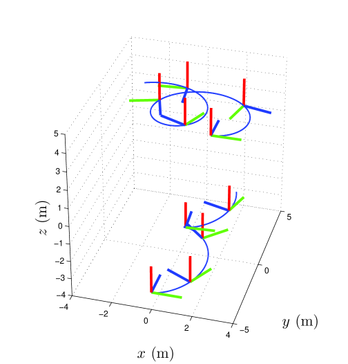
Figure 1: Position and attitude trajectory of the simulated vehicles.

Relative position vectors of these points are measured by the camera on the upper vehicle. Velocities of these points are calculated using the linear filter introduced in [10]. The relative velocities can be computed using these measurements by (9). All the camera readings contain random zero mean signals whose probability distributions are normalized bump functions with the width equal to 1 mm in each coordinate. The “inertia-like” gain matrices for the estimator are selected to be:

$$\begin{split}J&=\mbox{diag}\big{(}[0.9\;\;0.6\;\;0.3]^{\mbox{\small T}}\big{)},\\ M&=\mbox{diag}\big{(}[0.0608\;\;0.0486\;\;0.0365]^{\mbox{\small T}}\big{)}\end{split}$$ (35)

The “dissipation” gain matrices for the estimator are set to:

$$\begin{split}\mathbb{D}_{r}&=\mbox{diag}\big{(}[2.7\;2.2\;1.5]^{\mbox{\small T}}\big{)},\mathbb{D}_{t}=\mbox{diag}\big{(}[0.1\;\;0.12\;\;0.14]^{\mbox{\small T}}\big{)}.\end{split}$$ (36)

$\Phi(\cdot)$ could be any $C^{2}$ function with the properties described in Section 3, but is selected to be $\Phi(x)=x$ here. The initial estimated states have the following values:

$$\hat{R}_{0} =\operatorname{{expm}}_{\mathrm{SO(3)}}\big{(}(\frac{\pi}{4}\times[0\ 0\ 1]^{\mbox{\small T}})^{\times}\big{)},\;\hat{b}_{0}=[-3\;\;\;2\;\;\;4]^{\mbox{\small T}}\mbox{ m}$$

$$\hat{\omega}_{0} =[0.1\;\;-0.5\;\;\;0.05]^{\mbox{\small T}}\mbox{ rad/s},$$ (37)

an $$\mbox{d }\hat{\nu}_{0}=[0.05\;\;-0.09\;\;\;0.01]^{\mbox{\small T}}\mbox{ m/s}.$$

The discrete-time estimator (27)-(31) is simulated over a time interval of $T=10$ s with time stepsize $h=0.01$ s. At each instant, (27) is solved using Newton-Raphson iterations to find $F_{i}$. Then, the rest of the equations (all explicit) are solved consecutively to generate the estimated states. The principal angle of the relative attitude estimation error and components of the relative position estimate error are plotted in Fig. 2. Components of the relative angular and translational velocities are depicted in Fig. 3.

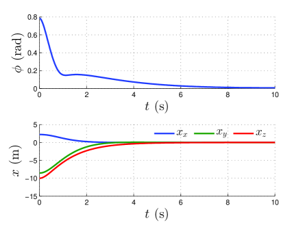
Figure 2: Principal angle of the relative attitude and position estimation error.

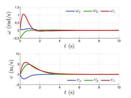
Figure 3: Relative angular and translational velocity estimation error.

As can be noticed from the figures, all the estimated relative states converge to a bounded neighborhood of the corresponding true relative states, where the size of this neighborhood depends on the level of measurement noise and estimator gains. This confirms the stability and convergence properties of the estimator.

6 CONCLUSION

This article proposes an estimator for relative pose and relative velocities of one vehicle with respect to another vehicle that uses only optical measurements from onboard optical sensor(s). The sensors are assumed to provide measurements in continuous-time or at a high frequency, with bounded measurement noise due to limited fields of view. A Lagrangian in terms of measurement residuals and which can be expressed in terms of state estimation errors when perfect measurements are available, is proposed. Applying the Lagrange-d’Alembert principle to this Lagrangian with a dissipation term linear in relative velocity estimation errors, an estimator is designed on the Lie group of relative motions between two rigid vehicles. In the case of perfect measurements, this estimator is shown to be almost globally asymptotically stable with a domain of convergence that is open and dense in the state space. The continuous estimator is discretized by applying the discrete Lagrange-d’Alembert principle to the discretized Lagrangian and dissipation terms for rotational and translational motions. In the presence of measurement noise, numerical simulations with this discrete estimator show that state estimates converge to a bounded neighborhood of the true relative motion states. Future work will be directed towards creating higher-order discretizations of the continuous-time filter given here.

References

- [1] Aguiar, A., & Hespanha, J. (2006). Minimum-energy state estimation for systems with perspective outputs. IEEE Transactions on Automatic Control, 51(2), 226–241.
- [2] Amelin, K. S., & Miller, A. B. (2014). An algorithm for refinement of the position of a light UAV on the basis of Kalman filtering of bearing measurements. Journal of Communications Technology and Electronics, 59(6), 622–631.
- [3] Bayadi, R., & Banavar, R. N. (2014). Almost global attitude stabilization of a rigid body for both internal and external actuation schemes. European Journal of Control, 20(1), 45–54.
- [4] Bonnabel, S., Martin, P., & Rouchon, P. (2009). Nonlinear symmetry-preserving observers on Lie groups. IEEE Transactions on Automatic Control, 54(7), 1709–1713.
- [5] Chaturvedi, N. A., Sanyal, A. K., & McClamroch, N. H. (2011). Rigid-body attitude control. IEEE Control Systems Magazine, 31(3), 30–51.
- [6] Goodarzi, F. A., Lee, D., & Lee, T. (2013). Geometric nonlinear PID control of a quadrotor UAV on SE(3). In Proceedings of the European Control Conference (pp. 3845–3850). Zurich, Switzerland.
- [7] Goodarzi, F. A., Lee, D., & Lee, T. (2014). Geometric Adaptive Tracking Control of a Quadrotor UAV on SE(3) for Agile Maneuvers. ASME Journal of Dynamic Systems, Measurement and Control, 137(9), 091007.
- [8] Goodarzi, F. A., Lee, D., & Lee, T. (2014). Geometric stabilization of a quadrotor UAV with a payload connected by flexible cable. In Proceedings of the American Control Conference (pp. 4925–4930). Portland, OR, USA.
- [9] Izadi, M., Samiei, E., Sanyal, A. K., & Kumar, V. (2015). Comparison of an attitude estimator based on the Lagrange-d’Alembert principle with some state-of-the-art filters. In Proceedings of the IEEE International Conference on Robotics and Automation (pp. 2848–2853). Seattle, WA, USA.
- [10] Izadi, M., Sanyal, A. K., Samiei, E., & Viswanathan, S. P. (2015). Discrete-time rigid body attitude state estimation based on the discrete Lagrange-d’Alembert principle. In Proceedings of the American Control Conference (pp. 3392–3397). Chicago, IL, USA.
- [11] Izadi, M., & Sanyal, A. K. (2014). Rigid body attitude estimation based on the Lagrange-d’Alembert principle. Automatica, 50(10), 2570–2577.
- [12] Izadi, M., & Sanyal, A. K. (2015). Rigid body pose estimation based on the Lagrange-d’Alembert principle. To appear in Automatica.
- [13] Khalil, H. K. (2001). Nonlinear Systems (3rd edition). Prentice Hall, Upper Saddle River, NJ.
- [14] Khosravian, A., Trumpf, J., Mahony, R., & Hamel, T. (2015). Recursive Attitude Estimation in the Presence of Multi-rate and Multi-delay Vector Measurements. In Proceedings of the American Control Conference (pp. 3199–3205). Chicago, IL, USA.
- [15] Khosravian, A., Trumpf, J., Mahony, R., & Lageman, C. (2015). Observers for invariant systems on Lie groups with biased input measurements and homogeneous outputs. Automatica, 55, 19–26.
- [16] Leishman, R. C., McLain, T. W., & Beard, R. W. (2014). Relative navigation approach for vision-based aerial GPS-denied navigation. Journal of Intelligent & Robotic Systems, 74(1-2), 97–111.
- [17] Mahony, R., Hamel, T., & Pflimlin, J. M. (2008). Nonlinear complementary filters on the special orthogonal group. IEEE Transactions on Automatic Control, 53(5), 1203–1218.
- [18] Maithripala, D. H., Berg, J. M., & Dayawansa, W. P. (2004). An intrinsic observer for a class of simple mechanical systems on a Lie group. In Proceedings of the American Control Conference (pp. 1546–1551). Boston, MA, USA.
- [19] Markley, F. L. (2006). Attitude filtering on SO(3). The Journal of the Astronautical Sciences, 54(4), 391–413.
- [20] Marsden, J. E., & West, M. (2001). Discrete mechanics and variational integrators. Acta Numerica, 10, 357–514.
- [21] Miller, A., & Miller, B. (2014). Tracking of the UAV trajectory on the basis of bearing-only observations. In Proceedings of the 53rd Annual Conference on Decision and Control (pp. 4178–4184). Los Angeles, CA, USA.
- [22] Misra, G., Izadi, M., Sanyal, A. K., & Scheeres, D. J. (2015). Coupled orbit-attitude dynamics and relative state estimation of spacecraft near small Solar System bodies. Advances in Space Research.
- [23] Mortensen, R. E. (1968). Maximum-likelihood recursive nonlinear filtering. Journal of Optimization Theory and Applications, 2(6), 386–394.
- [24] Rehbinder, H., & Ghosh, B. K. (2003). Pose estimation using line-based dynamic vision and inertial sensors. IEEE Transactions on Automatic Control, 48(2), 186–199.
- [25] Sanyal, A. K., Fosbury, A., Chaturvedi, N. A., & Bernstein, D. S. (2009). Inertia-free spacecraft attitude tracking with disturbance rejection and almost global stabilization. Journal of Guidance, Control, and Dynamics, 32(4), 1167–1178.
- [26] Sanyal, A. K., Izadi, M., & Butcher, E. A. (2014). Determination of relative motion of a space object from simultaneous measurements of range and range rate. In Proceedings of the American Control Conference (pp. 1607–1612). Portland, OR, USA.
- [27] Sanyal, A. K., Lee, T., Leok, M., & McClamroch, N. H. (2008). Global optimal attitude estimation using uncertainty ellipsoids. Systems & Control Letters, 57(3), 236–245.
- [28] Shen, S., Mulgaonkar, Y., Michael, N., & Kumar, V. (2013). Vision-based state estimation and trajectory control towards aggressive flight with a quadrotor. In Proceedings of the Robotics Science and Systems.
- [29] Shen, S., Mulgaonkar, Y., Michael, N., & Kumar, V. (2013). Vision-based state estimation for autonomous rotorcraft MAVs in complex environments. In Proceedings of the IEEE International Conference on Robotics and Automation (pp. 1758–1764). Karlsruhe, Germany.
- [30] Tayebi, A., Roberts, A., & Benallegue, A. (2011). Inertial measurements based dynamic attitude estimation and velocity-free attitude stabilization. In Proceedings of the American Control Conference (pp. 1027–1032). San Francisco, CA, USA.
- [31] Vasconcelos, J. F., Cunha, R., Silvestre, C., & Oliveira, P. (2010). A nonlinear position and attitude observer on SE(3) using landmark measurements. Systems & Control Letters, 59, 155–166.
- [32] Vasconcelos, J. F., Silvestre, C., & Oliveira, P. (2008). A nonlinear GPS/IMU based observer for rigid body attitude and position estimation. In Proceedings of the IEEE Conference on Decision and Control (pp. 1255–1260). Cancun, Mexico.
- [33] Wahba, G. (1965). A least squares estimate of satellite attitude, Problem 65-1. SIAM Review, 7(5), 409.
- [34] Zamani, M. (2013). Deterministic Attitude and Pose Filtering, an Embedded Lie Groups Approach. Ph.D. Thesis. Australian National University, Canberra, Australia.
- [35] Zamani, M., Trumpf, J., & Mahony, R. (2013). Minimum-energy filtering for attitude estimation. IEEE Transactions on Automatic Control, 58(11), 2917–2921.