Pattern formation in flocking models: A hydrodynamic description

Abstract

We study in detail the hydrodynamic theories describing the transition to collective motion in polar active matter, exemplified by the Vicsek and active Ising models. Using a simple phenomenological theory, we show the existence of an infinity of propagative solutions, describing both phase and microphase separation, that we fully characterize. We also show that the same results hold specifically in the hydrodynamic equations derived in the literature for the active Ising model and for a simplified version of the Vicsek model. We then study numerically the linear stability of these solutions. We show that stable ones constitute only a small fraction of them, which however includes all existing types. We further argue that in practice, a coarsening mechanism leads towards phase-separated solutions. Finally, we construct the phase diagrams of the hydrodynamic equations proposed to qualitatively describe the Vicsek and active Ising models and connect our results to the phenomenology of the corresponding microscopic models.

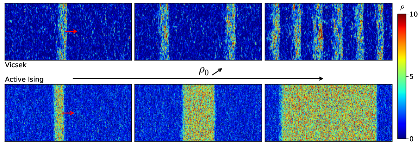
Figure 1: Top: Micro-phase separation in the Vicsek model. $\eta=0.4$, $v_{0}=0.5$, $\rho_{0}=0.83,\,1.05,\,1.93$. Bottom: Phase separation in the Active Ising model. $D=1$, $\varepsilon=0.9$, $\beta{}=1.9$, $\rho_{0}=1.5,\,2.35,\,4.7$. System sizes $800\times 100$. High-density bands propagate as indicated by the red arrows on the left snashots.

I Introduction

Collective motion is the ability of large groups of motile agents to move coherently on scales much larger than their individual sizes. It is encountered at all scales in nature, from macroscopic animal groups, such as bird flocks, fish schools, or sheep herds, down to the cellular scale, where the collective migration of cells HakimCells or bacteria PeruaniMB is commonly observed. At the subcellular level, in vitro motility assays of actin filaments Schaller2010 or microtubules SuminoNature2010 have shown the spontaneous emergence of large vortices. Collective motion is also observed in ensemble of man-made motile particles such as shaken polar grains DauchotDisks , colloidal rollers Rollers , self-propelled droplets Thutupalli or assemblies of polymers and molecular motors Schaller2010 ; SuminoNature2010 ; Sanchez2012 . Despite the differences in their propulsion and interaction mechanisms, these seemingly very different systems share common macroscopic behaviors that can be captured by minimal physical models. Of particular interest is the emergence of directed collective motion, which was first addressed in this context in a seminal work by Vicsek and co-workers Vicsek . The Vicsek model consists in point particles moving at constant speed and aligning imperfectly with the direction of motion of their neighbors. When the error on the alignment interaction is decreased, or the density of particles increased, a genuine phase transition from a disordered to a symmetry-broken state is observed. This flocking transition gives rise to an emergent ordered phase, with true long-range polar order even in 2D, where all the particles propel on average along the same direction. Toner and Tu showed analytically, using a phenomenological fluctuating hydrodynamic description, how this ordered state, which would be forbidden by the Mermin-Wagner theorem at equilibrium MerminWagner , is stabilized by self-propulsion TT . The transition to collective motion in the Vicsek model has a richer phenomenology than originally thought. As first pointed out numerically in ChateGregoire , at the onset of collective motion, translational symmetry is broken as well. In periodic simulation boxes, high-density ordered bands of particles move coherently through a low-density disordered background. The transition between these bands and the homogeneous disordered profile is discontinuous, with metastability and hysteresis loops. These spatial patterns and the first-order nature of the transition can be encompassed in a wider framework, which describes the emergence to collective motion as a liquid-gas phase separation AIM ; Microphase . The travelling bands result from the phase coexistence between a disordered gas and an ordered polarized liquid. This framework captures many of the characteristics of the transition, from the scaling of the order parameter to the shape of the phase diagram. This phase-separation picture is robust to the very details of the propulsion and interaction mechanisms. More specifically, it has also been quantitatively demonstrated in the active Ising model AIM in which particles can diffuse in a 2d space but self-propel, and align, only along one axis. However the specifics of the emergent spatial patterns and the type of phase separation depend on the symmetry of the orientational degrees of freedom. While the active Ising model model shows a bulk phase separation, the Vicsek model is akin to an active XY model and is associated with a microphase separation where the coherently moving polar patterns self-organize into smectic structures Microphase (see Fig. 1).

In this paper, building on the two prototypical models that are the Vicsek model and the active Ising model, we provide a comprehensive description of the emergent patterns found at the onset of the flocking transition from a hydrodynamic perspective. We first recall the definitions and phenomenologies of these two models in Sec. II. In Sec. III, we provide a simplified hydrodynamic description of the flocking models. In line with Bertin ; Caussin , we show that these models support non-linear propagative solutions whose shape is described using a mapping onto the trajectories of point-like particles in one-dimensional potentials. Finding such solutions thus reduces to a classical mechanics problem with one degree of freedom. For given values of all the hydrodynamic coefficients, and hence of all underlying microscopic parameters, we find an infinity of solutions, describing both phase and microphase separations, that we fully characterize. We then show that the same results hold specifically for the hydrodynamic equations explicitly derived for the active Ising model AIM and for a simplified version of the Vicsek model Bertin . Next, we investigate the linear stability of these solutions as solutions of the hydrodynamic equations in Sec. VI and their coarsening dynamics in Sec. VII. Finally, we provide full phase diagrams constructed from the hydrodynamic model in Sec. VIII. We close by discussing the similarities and differences with the phenomenology of the agent-based models and conjecture on the role of the hydrodynamic noise in the selection of the band patterns.

II Phenomenology of microscopic models

Let us first briefly recall the phenomenology of the Vicsek and active Ising models. They are both based on the same two ingredients: Self-propulsion and a local alignment rule. The major differences between the two models are thus the symmetries of the alignment interaction and of the direction of motion.

II.1 Vicsek model

In the Vicsek model Vicsek , $N$ point-like particles, labeled by an index $i$, move at constant speed $v_{0}$ on a rectangular plane with periodic boundary conditions. At each discrete time step $\Delta t=1$, the headings $\theta_{i}$ of all particles are updated in parallel according to

$$\theta_{i}(t+1)=\langle\theta_{j}(t)\rangle_{j\in\mathcal{N}_{i}}+\eta\,\xi_{i}^{t}$$ (1)

where $\mathcal{N}_{i}$ is the disk of unit radius around particle $i$, $\xi_{i}^{t}$ a random angle drawn uniformly in $[-\pi,\pi]$, and $\eta$ sets the level of noise, playing a role akin to that of a temperature in a ferromagnetic XY model. Then, particles hop along their new headings: ${\bf r}_{i}(t+1)={\bf r}_{i}(t)+v_{0}{\bf e}_{i}^{t+1}$, where ${\bf e}_{i}^{t+1}$ is the unit vector pointing in direction given by $\theta_{i}({t+1})$.

II.2 Active Ising model

In the active Ising model AIM , particles carry a spin $\pm 1$ and move on a 2D lattice with periodic boundary conditions. Their dynamics depend on the sign of their spin: A particle with spin $s$ jumps to the site on its right at rate $D(1+s\varepsilon)$ and to the site on its left at rate $D(1-s\varepsilon)$, where $0\leq\varepsilon\leq 1$ measures the bias on the diffusion. On average, $+1$ particles thus self-propel to the right and $-1$ particles to the left at a mean velocity $v_{0}\equiv 2D\varepsilon$. Both types of particles diffuse symetrically at rate $D$ in the vertical direction.

The alignment interaction is purely local. On a site $i$, a particle flips its spin $s$ at rate

$$W_{i}(s\to-s)=\exp\left(-\frac{s}{T}\frac{m_{i}}{\rho_{i}}\right)$$ (2)

where $T$ is a temperature, and $m_{i}$ and $\rho_{i}$ are the magnetization and number of particles on site $i$. (An arbitrary number of particles is allowed on each site since there is no excluded volume interaction.)

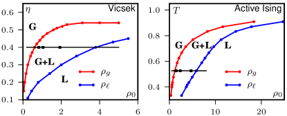
Figure 2: Phase diagrams of the microscopic models. The red and blue lines delimit the domain of existence of (micro) phase-separated profiles. The black line and squares indicate the position of the snapshots shown in Fig. 1. $v_{0}=0.5$ for the Vicsek model, $D=1$ and $\varepsilon=0.9$ for the active Ising model.

II.3 A liquid-gas phase transition

The phase diagrams in the temperature/noise-density ensemble are shown for both models in Fig. 2, highlighting their similarity. At high temperature/noise or low density both systems are in a homogeneous disordered gas state. At low temperature/noise and high density they are homogeneous and ordered; in these liquid phases, all particles move in average in the same direction. In the central region of the phase diagram, inhomogeneous profiles are observed, with liquid domains moving in a disordered gaseous background.

The phase transitions of both models have all the features of a liquid-gas transition, exhibiting metastability and hysteresis close to the transition lines ChateGregoire ; AIM ; Microphase . The main difference between the two models lies in the coexistence region: In the active Ising model, the particles phase separate in a gaseous background and an ordered liquid band, both of macroscopic sizes AIM . The coexisting densities depend only on temperature and bias, but not on the average density; in the coexistence region, increasing the density at fixed $T,\varepsilon$ thus results in larger and larger liquid domains whose density remains constant, as shown in Fig. 1. Conversely, in the Vicsek model, the system forms arrays of ordered bands arranged periodically in space which have a finite width along their direction of motion: a micro-phase separation occurs Microphase . As shown in Fig. 1, increasing the density at constant noise, the number of bands increases but their shape does not change Microphase .

Three types of propagating patterns can thus be observed at phase coexistence, all shown in Fig. 1: (i) localized compact excitations, (ii) Smectic microphases, and (iii) Phase-separated polar liquid domains. In the vicinity of the left coexistence line, collective motion emerges in the form of localized compact excitations in both models foot1 . At higher density, phase-separated domains are found in the active Ising model and periodic “smectic” bands in the Vicsek model. Understanding the emergence of these three types of solutions will be the focus of the rest of the paper.

III Hydrodynamic Equations

A lot of attention has been given in the literature to hydrodynamic equations of flocking models. Two different approaches have been followed, starting from phenomenological equations TT ; Baskaran ; Caussin or deriving explicitly coarse-grained equations from a microscopic model Bertin ; Ihle ; Farrell ; Pawel ; AIM . All these equations describe the dynamics of a conserved density field $\rho(\vec{r},t)$ coupled to a non-conserved magnetization field, the latter being a vector $\vec{m}(\vec{r},t)$ for continuous rotational symmetries, as in the Vicsek model, or a scalar $m(\vec{r},t)$, for discrete symmetries, as in the active Ising model.

We first introduce in Sec. III.1 two sets of hydrodynamic equations derived by coarse-graining microscopic models which will be discussed in this paper. Then, we turn in Sec. III.2 to a simpler set of phenomenological hydrodynamic equations on which we will establish our general results in Sec. IV.

III.1 Coarse-grained hydrodynamic descriptions

We first consider the equations proposed by Bertin et al. to describe a simplified version of the Vicsek model Bertin , in which one solely considers binary collisions between the particles. One can then use, assuming molecular chaos, a Boltzmann equation formalism to arrive at the following hydrodynamic equations for the density field and a vectorial magnetization field foot3

$$\frac{\partial\rho}{\partial t} =-v_{0}\nabla\cdot\vec{m}$$ (3)

$$\frac{\partial\vec{m}}{\partial t} +\gamma(\vec{m}\cdot\nabla)\vec{m}=\nu\nabla^{2}\vec{m}-\frac{v_{0}}{2}\nabla\rho+\frac{\kappa}{2}\nabla(|\vec{m}|^{2})$$

$$\qquad\qquad\qquad-\kappa(\nabla\cdot\vec{m})\vec{m}+(\mu-\zeta|\vec{m}^{2}|)\vec{m}$$ (4)

The mass-conservation equation (3) simply describes the advection of the density by the magnetization field. Equation (III.1) can be seen as a Navier-Stokes equation complemented by a Ginzburg-Landau term $(\mu-\zeta|\vec{m}|^{2})\vec{m}$, stemming from some underlying alignment mechanism, and leading to the emergence of a spontaneous magnetization. Because particles are self-propelled in a given frame of reference, these equations break Galilean invariance so that one can have $\gamma\neq 1$ and $\kappa\neq 0$ unlike e.g. in the Navier-Stokes equation.

In Eqs. (3) and (III.1), to which we refer to as “Vicsek hydrodynamic equations” hereafter, all the coefficients $\gamma$, $\nu$, $\kappa$, $\mu$ and $\zeta$, depend on the local density; see Bertin for their exact expression.

The second set of equations, which we refer to as “Ising hydrodynamic equations” in the following, has been derived to describe the large-scale phenomenology of the active Ising model AIM . In this case, the dynamics of the density field and the scalar magnetization—corresponding to the Ising symmetry—are given by

$$\frac{\partial\rho}{\partial t} =D\Delta\rho-v_{0}\partial_{x}m$$ (5)

$$\frac{\partial m}{\partial t} =D\Delta m-v_{0}\partial_{x}\rho+2\left(\beta{}-1-\frac{r}{\rho}\right)m-\alpha\frac{m^{3}}{\rho^{2}}$$ (6)

where $\beta=1/T$, $\alpha$ and $r$ are positive coefficients depending on $\beta{}$ only and $v_{0}=2D\varepsilon$. The advection term $v_{0}\nabla\vec{m}$ of Eq. (3) is here replaced by a partial derivative $v_{0}\partial_{x}m$ because, in the active Ising model, the density is advected by the magnetization only in the $x$-direction.

III.2 Phenomenological hydrodynamic equations with constant coefficients

Coarse-grained hydrodynamic equations derived from microscopic models have the advantage of expressing the macroscopic transport coefficients in terms of microscopic quantities (noise, self-propulsion speed, etc). However, these possibly complicated relations may not be relevant to understand the qualitative behavior of the models. Thus, before discussing the Vicsek and Ising hydrodynamic equations in Sec. V, we first study in detail, in Sec. IV, a simpler model

$$\partial_{t} \rho=-v_{0}\nabla\cdot\vec{m}$$ (7)

$$\partial_{t} \vec{m}+\xi(\vec{m}\cdot\nabla)\vec{m}=D\nabla^{2}\vec{m}-\lambda\nabla\rho+a_{2}\vec{m}-a_{4}|\vec{m}|^{2}\vec{m}$$ (8)

where the transport coefficients $v_{0}$, $\xi$, $D$, $\lambda$ and $a_{4}$ are constant. In the following, we refer to these equations as the “phenomenological hydrodynamic equations”. This simplified model is very similar to that first introduced by Toner and Tu from symmetry considerations TT . However, unlike the original Toner and Tu model, we keep an explicit density dependence in $a_{2}$: $a_{2}(\rho)=\rho-\varphi_{g}$, which is essential to account for inhomogeneous profiles Bertin ; Baskaran ; AIM .

The stability criteria of the homogeneous solutions ($\rho(\textbf{r},t)=\rho_{0}$, $\vec{m}(\textbf{r},t)=\vec{m}_{0}$) of Eqs. (7-8) are readily computed:

• For $\rho_{0}<\varphi_{g}$ ($a_{2}(\rho_{0})<0$) only the disordered solution ($\rho_{0}$, $|\vec{m}_{0}|=0$) exists and is stable

• For $\rho_{0}>\varphi_{g}$ ($a_{2}(\rho_{0})>0$) the disordered solution becomes unstable and ordered solutions ($\rho_{0}$, $|\vec{m}_{0}|=\sqrt{(\rho_{0}-\varphi_{g})/a_{4}}$) appear.

• The ordered solutions are linearly stable only when $\rho_{0}>\varphi_{\ell}=\varphi_{g}+\frac{1}{4a_{4}v_{0}+2\lambda}$

Thus, in the range $\rho_{0}\in[\varphi_{g},\varphi_{\ell}]$, homogeneous solutions are linearly unstable. In the language of the liquid-gas transition, $\varphi_{g}$ and $\varphi_{\ell}$ are the gas and liquid spinodals, between which the homogeneous phases are linearly unstable and spinodal decomposition takes place. In the next section we address the existence of heterogenous ordered excitations propagating through stable disordered (gaseous) backgrounds. This analysis will make it possible both to identify all the possible flocking patterns and to further understand the first-order nature of the flocking transition.

IV Propagative solutions

Let us now establish and classify all the inhomogeneous propagating solutions of Eqs. (7-8). In order to do so, we first recast this problem into a dynamical system framework in section IV.1. We then show in section IV.2 that three types of propagating solutions exist with different celerities $c$ and densities of the gaseous background $\rho_{g}$. Sections IV.3, IV.4 and IV.5 are dedicated to a detailed study of how these solutions depend on $c$ and $\rho_{g}$. Section IV.6 shows how, once the average density is fixed, we are left with a one-parameter family of solutions. Last, section IV.7 is devoted to cases where the inhomogeneous profiles can be studied analytically.

IV.1 Newton Mapping

Following Bertin , we look for inhomogeneous polar excitations invariant along, say the $y$ direction, and which propagate, and/or relax solely along the $x$ direction. We thus assume, $m_{y}=0$ and reduce Eqs. (7-8) to:

$$\partial_{t} \rho=-v_{0}\partial_{x}m$$ (9)

$$\partial_{t} m+\xi m\partial_{x}m=D\partial_{x}^{2}m-\lambda\partial_{x}\rho+(\rho-\varphi_{g})m-a_{4}m^{3}$$ (10)

where we wrote $m=m_{x}$ to ease the notation. We look for solutions propagating steadily at a speed $c$. Introducing the position $z=x-ct$ in the frame moving at $c$: $\rho(x,t)=\rho(z)$, $m(x,t)=m(z)$, we obtain

$$c \dot{\rho}-v_{0}\dot{m}=0$$ (11)

$$D \ddot{m}+(c-\xi m)\dot{m}-\lambda\dot{\rho}+(\rho-\varphi_{g})m-a_{4}m^{3}=0$$ (12)

where the dots denote derivation with respect to $z$. Solving Eq. (11) gives $\rho(z)=\rho_{g}+\frac{v_{0}}{c}m(z)$. If $\rho(z)$ is localized in space, $\rho_{g}$ has a simple meaning. Since $\rho(z)=\rho_{g}$ when $m(z)=0$, the integration constant $\rho_{g}$ is the density in the gaseous phase surrounding the localized polar excitation. We can then insert the expression of $\rho$ in Eq. (12) and obtain the second-order ordinary differential equation

$$D\ddot{m}+(c-\frac{\lambda v_{0}}{c}-\xi m)\dot{m}-(\varphi_{g}-\rho_{g})m+\frac{v_{0}}{c}m^{2}-a_{4}m^{3}=0$$ (13)

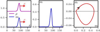
Figure 3: Left: Density and magnetization profiles of a propagative solution of the hydrodynamic Eqs. (7-8). Center: Magnetization profile in the comoving frame $z=x-ct$ or, equivalently, trajectory $m(z)$ of a point particle in the spurious time $z$. Right: Phase portrait corresponding to the trajectory $m(z)$. Parameters: $D=v_{0}=\lambda=\xi=a_{4}=\varphi_{g}=1$.

Following Bertin ; Caussin , we now provide a mechanical interpretation of Equation (13) through the well-known Newton mapping. Rewriting Eq. (13) as:

$$D\ddot{m} =-f(m)\dot{m}-\frac{dH}{dm}$$ (14)

$$H(m) =-(\varphi_{g}-\rho_{g})\frac{m^{2}}{2}+\frac{v_{0}}{3c}m^{3}-\frac{a_{4}}{4}m^{4}$$ (15)

$$f(m) =c-\frac{\lambda v_{0}}{c}-\xi m$$ (16)

it is clear that this equation corresponds to the mechanical equation of motion of a point particle. The position of the particle is $m$, $z$ is the time variable, $D$ is the mass of the particle, $H(m)$ is an energy potential and $f(m)$ is a position-dependent friction. The trajectory $m(z)$ of this fictive particle exactly corresponds to the shape of the propagative excitations of our hydrodynamic model in the frame moving at a speed $c$ (see Fig. 3).

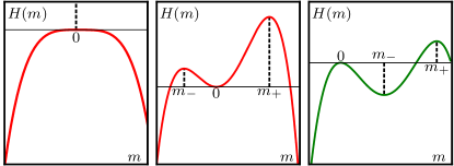
Figure 4: The green potential can give rise to physical (positive, non-exploding) solutions while the red ones are ruled out by our conditions (C1) (left) and (C2) (center).

We shall stress that for a given hydrodynamic model, Eq. (14) is parametrized by the two unknown parameters $c$ and $\rho_{g}$ which a priori can take any value. Each pair ($c$, $\rho_{g}$) gives different potential $H$ and friction $f$, and hence different trajectories $m(z)$. We now turn to the study of these trajectories and of the corresponding admissible values for the celerity $c$ and the gas density $\rho_{g}$.

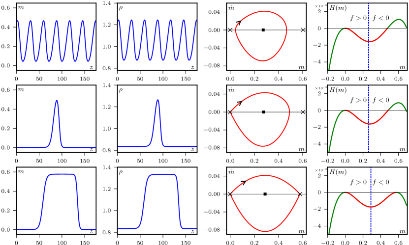
Figure 5: Example of the three types of trajectories. From left to right: magnetization and density profiles, phase portrait, and potential $H$. Top row: Periodic trajectory, $\rho_{g}=0.835$, $c=1.14$. Center row: Homoclinic trajectory, $\rho_{g}=0.83412$, $c=1.14$. Bottom row: Heteroclinic trajectory, $\rho_{g}=0.83333$, $c=1.1547$. Phase portrait: Crosses indicate saddle points at $m=0$ and $m=m_{+}$. Squares indicate stable fixed points at $m=m_{-}$. Potentials: The blue dashed line indicate where the friction changes sign. The red portion of the potential is the one visited by the trajectory. Parameters: $D=v_{0}=\lambda=\xi=a_{4}=\varphi_{g}=1$.

IV.2 Three possible propagating patterns

The original problem of finding all the inhomogeneous propagative solutions $m(x,t)$, $\rho(x,t)$ of the hydrodynamic equations is now reduced to finding all the pairs ($c$, $\rho_{g}$) for which the corresponding trajectories $m(z)$ exist. Mass conservation, Eq. (9), imposes the boundary condition $m(z=-\infty)=m(z=+\infty)$ so that we are looking for solutions of (14) which are closed in the $(m,\dot{m})$ plane. An example of propagative solutions $m(x,t)$, $\rho(x,t)$ together with the corresponding trajectory $m(z)$ and its phase portraits is shown in Fig. 3.

To put a first constraint on $\rho_{g}$ and $c$, let us rule out the potentials which cannot give such physical solutions. The extrema of $H$, solutions of $H^{\prime}(m)=0$, are located at $m=0$ and $m=m_{\pm}$ with

$$m_{\pm}=\frac{v_{0}}{2a_{4}c}\left(1\pm\sqrt{1-\frac{4a_{4}(\varphi_{g}-\rho_{g})c^{2}}{v_{0}^{2}}}\right)$$ (17)

We can already discard the case where $H^{\prime}(m)$ has two complex roots since $H$ then has a single maximum at $m=0$, and all trajectories wander to $m=\pm\infty$ (see Fig. 4, left). This leads to a first condition on $c$, $\rho_{g}$:

$$(\varphi_{g}-\rho_{g})c^{2}<a_{4}v_{0}^{2}$$ (C1)

Without loss of generality we can assume that $c>0$ and look only for solutions with $m\geq 0$. This rules out the ($c$, $\rho_{g}$) values for which $m_{-}<0$ and $m_{+}>0$ which give oscillations between negative and positive values of $m$ (see Fig. 4, central panel). At the hydrodynamic equation level, such solutions would indeed correspond to different parts of the profiles moving in opposite direction. The corresponding condition

$$\rho_{g}<\varphi_{g}$$ (C2)

imposes $0<m_{-}<m_{+}$. The potential $H$ then has two maxima, at $m=0$ and $m=m_{+}$, and one minimum, at $m=m_{-}$. The typical shape of potential which gives admissible solutions is shown in Fig. 4 along with examples of potentials ruled out by conditions (C1) and (C2).

>From the admissible shape of the potential $H$, we can now list all possible trajectories $m(z)$ and the corresponding fields $m(x,t)$, $\rho(x,t)$:

• Limit cycles, whose corresponding magnetisation profiles are periodic bands, as shown in the first row of Fig. 5.

• Homoclinic orbits, that start infinitely close to a maximum of $H$, hence spending an arbitrary large time there, before crossing twice the potential well in a finite time to finally return to the same maximum of $H$ at $z=\infty$. These trajectories correspond to isolated solitonic band profiles, as shown in the second row of Fig. 5.

• Heteroclinic orbits that spend an arbitrary large time close to a first maximum of $H$, cross the potential well in a finite time, spend an arbitrary large time close to the second maximum of $H$, before returning to the first maximum. These trajectories correspond to phase separated profiles. The arbitrary waiting times at the two maxima of $H$ then reflect the arbitrary sizes of two phase-separated domains (see the third row of Fig. 5).

A third condition on $\rho_{g},c$ arises from the non-linear friction term. Following the classical mechanics analogy, we define an energy function

$$E=\frac{1}{2}D\dot{m}^{2}+H$$ (18)

Multiplying the equation of motion (13) by $\dot{m}$, we get

$$\frac{dE}{dz}=-f(m)\dot{m}^{2}$$ (19)

Energy is injected when $f(m)<0$ and dissipated when $f(m)>0$. On a closed trajectory, the friction $f$ must thus change sign. Since $f$ is a decreasing function of $m$, this imposes $f(0)>0$ for trajectories with $m(z)>0$, or equivalently

$$c>\sqrt{\lambda v_{0}}$$ (C3)

The conditions (C1), (C2) and (C3) thus provide loose bounds on the subspace of the ($c,\rho_{g}$) plane which contains the three types of trajectories $m(z)$ described above. These trajectories correspond to the three types of inhomogeneous profiles seen in the microscopic models foot2 . Before studying the stability and coarsening of these propagative solutions, we first need to understand precisely how they are organised in the ($c$, $\rho_{g}$) plane. In order to do so, we first analyze the phase portrait of the dynamics (14). We then study how the phase portrait evolves when $\rho_{g}$ and $c$ are varied.

IV.3 Stability of the fixed points

The structure of the phase portrait is most easily captured by locating the fixed points of  (14) and studying their stability. We first rewrite (14) as a system of two first-order differential equations:

$$\frac{d}{dz}\begin{pmatrix}m\\ \dot{m}\end{pmatrix}=\begin{pmatrix}\dot{m}\\ -\frac{f(m)}{D}\dot{m}-\frac{H^{\prime}(m)}{D}\end{pmatrix}$$ (20)

The fixed points are the solutions satisfying $\dot{m}=0$ and $H^{\prime}(m)=0$, i.e., the constant solutions extremizing $H$. As explained before, because of the condition (C2), the extrema of $H$ at $m=0,m_{-},m_{+}$ are such that $0<m_{-}<m_{+}$, so that $0$ and $m_{+}$ are two maxima and $m_{-}$ is a minimum of $H$.

Linearizing the dynamics around one of the fixed points, we define $m=m_{0}+\delta m$ with $m_{0}=0,\,m_{-},m_{+}$, so that $\dot{m}=\dot{\delta m}$ and

$$\frac{d}{dz}\begin{pmatrix}\delta m\\ \dot{\delta m}\end{pmatrix}=\begin{pmatrix}0&1\\ -H^{\prime\prime}(m_{0})/D&-f(m_{0})/D\end{pmatrix}\begin{pmatrix}\delta m\\ \dot{\delta m}\end{pmatrix}$$ (21)

The stability of the fixed points is given by the eigenvalues $\lambda_{1,2}$ of the $2\times 2$ matrix which read

$$\lambda_{1,2}(m_{0})=\frac{-f(m_{0})}{2D}\pm\sqrt{\left(\frac{f(m_{0})}{2D}\right)^{2}-\frac{H^{\prime\prime}(m_{0})}{D}}$$ (22)

• At the maxima $m_{0}=0$ and $m_{0}=m_{+}$ of $H$, $H^{\prime\prime}(m_{0})$ is negative and the two eigenvalues are thus real with opposite signs. These fixed points are saddle points with one unstable direction ($\lambda_{1}>0$) and one stable direction ($\lambda_{2}<0$).

• At the minimum $m_{0}=m_{-}$ of $H$, $H^{\prime\prime}(m_{0})$ is positive and the real part of the two eigenvalues have the same sign, given by $-f(m_{-})$. The fixed point is stable when $f(m_{-})>0$ and unstable when $f(m_{-})<0$. Physically, when the friction of the fictive particle is negative around $m=m_{-}$, small perturbations are amplified, driving the trajectory away from the fixed point. Conversely, a positive friction damps any initial perturbation, leading to trajectories converging towards $m_{-}$.

  When $c$ and $\rho_{g}$ are such that $f(m_{-})=0$, $\lambda_{1,2}$ are complex conjugate imaginary numbers. A Hopf bifurcation takes place, leading to the apparition of a limit cycle.

At the onset of a Hopf bifurcation, a limit cycle appears around the fixed point whose stability changes. In the following sections we elucidate how the interplay between the saddle-point and the Hopf dynamics rules the non-linear dynamics of the fictive particle and hence the polar-band shape.

IV.4 Hopf bifurcation

Let us first provide a comprehensive characterization of the Hopf bifurcation. It happens when the real part of $\lambda_{1,2}$ vanishes, i.e., when

$$f(m_{-})=c-\frac{\lambda v_{0}}{c}-\xi m_{-}(c,\rho_{g})=0$$ (23)

where $m_{-}$, which depends on both $c$ and $\rho_{g}$, is given by Eq. (17). Equation (23) is satisfied on the line

$$\rho_{g}^{H}(c)=\varphi_{g}+\frac{(-c^{2}+v_{0}\lambda)(-a_{4}c^{2}+a_{4}v_{0}\lambda+v_{0}\xi)}{c^{2}\xi^{2}}$$ (24)

which we call the Hopf transition line.

Figure 6: The four types of phase portrait ($m$, $\dot{m}$) obtained in our system when changing $\rho_{g}$ and $c$. The line $\rho_{g}=\rho_{g}^{H}$ is where the Hopf bifurcation takes place. The bifurcation is supercritical for $c<c^{*}$ and subcritical for $c>c^{*}$. The plain (resp. open) black squares denote stable (resp. unstable) fixed points at $m=m_{-}$. The plain (resp. dashed) black lines denote stable (resp. unstable) limit cycles. The crosses denote the saddle points at $m=0$ and $m=m_{+}$. The initial condition of each trajectory is marked by a magenta disk and the direction of “time” $z$ indicated by a magenta arrow.

Following standard text books in bifurcation theory Bifurcation , the type of Hopf bifurcation (super- or sub-critical) is given by the sign of

$$\Delta=\frac{\xi^{2}}{16\omega D^{3}}H^{\prime\prime\prime}(m_{-},\rho_{g}^{H})\frac{\partial m_{-}}{\partial\rho_{g}}(\rho_{g}^{H})$$ (25)

where $\omega=\sqrt{H^{\prime\prime}(m_{-},\rho_{g}^{H})/D}>0$ is the imaginary part of the eigenvalues at the bifurcation point. Moreover

$$\frac{\partial m_{-}}{\partial\rho_{g}}=\frac{-1}{\sqrt{\frac{v_{0}^{2}}{c^{2}}-4a_{4}(\varphi_{g}-\rho_{g})}}$$ (26)

is always negative because of condition (C1). The sign of $\Delta$ is thus given by the sign of $H^{\prime\prime\prime}(m_{-},\rho_{g}^{H})$, which changes at $c=c^{*}$ with

$$c^{*}=\frac{\sqrt{v_{0}(3a_{4}\lambda+\xi)}}{\sqrt{3a_{4}}}$$ (27)

Two different scenarios occur depending on whether $c$ is larger or smaller than $c^{*}$.

• When $c<c^{*}$, the Hopf bifurcation is supercritical ($\Delta>0$). The system branches from a stable fixed point for $\rho_{g}>\rho_{g}^{H}$ (case I, Fig. 6) to a stable limit cycle surrounding an unstable fixed point for $\rho_{g}<\rho_{g}^{H}$ (case II, Fig. 6).

• When $c>c^{*}$, the Hopf bifurcation is subcritical ($\Delta<0$). The system branches from an unstable fixed point when $\rho_{g}<\rho_{g}^{H}$ (case IV, Fig. 6) to an unstable limit cycle surrounding a stable fixed point when $\rho_{g}>\rho_{g}^{H}$ (case III, Fig. 6).

The organisation of these four typical cases in the $(c,\rho_{g})$ plane is illustrated in Fig. 6. We thus see that, when $c<c^{*}$, limit cycles exist for $\rho_{g}$ smaller than $\rho_{g}^{H}$, whereas when $c>c^{*}$, they exist for $\rho_{g}$ larger than $\rho_{g}^{H}$. The Hopf bifurcation line is thus a boundary of the domain of existence of periodic propagative solutions of the hydrodynamic equations. Let us now consider what happens when we explore the $c,\rho_{g}$ plane further away from the Hopf bifurcation line.

IV.5 Structure of the ($c$, $\rho_{g}$) solution space

So far, we have shown that three different types of trajectories $m(z)$ (periodic, homoclinic and heteroclinic) can be found by varying the values of $c$, $\rho_{g}$. The subspace where these physical solutions can be found was first bounded by the conditions (C1), (C2), and  (C3). In the previous section, we further found that the Hopf transition line $\rho_{g}^{H}(c)$ given by Eq. (24) is the upper boundary for the admissible values of $\rho_{g}$ when $c<c^{*}$ and the lower boundary when $c>c^{*}$.

To explore the remaining ($c$, $\rho_{g}$) space, we numerically integrated the dynamical system (20) using a Runge-Kutta scheme of order 4. Starting from different initial conditions, one easily finds the basins of attraction of the different solutions. To locate unstable fixed points and limit cycles, we integrated the dynamics backward in time since they are attractors when $z\to-\infty$. As $c$ and $\rho_{g}$ vary, so do the shapes and sizes of the limit cycles. To quantify these variations, we measured the “amplitude” of a cycle, defined as the difference between the two extrema of $m(z)$

$$\Delta m\equiv\underset{z}{{\rm max}}[m(z)]-\underset{z}{{\rm min}}[m(z)]$$ (28)

We systematically vary $\rho_{g}$ at fixed $c$, first focussing on the case $c<c^{*}$ where the Hopf bifurcation is supercritical. Decreasing $\rho_{g}$, a stable limit cycle of vanishing amplitude appears at $\rho_{g}=\rho_{g}^{H}$ (Fig. 7, panel A). The amplitude of the cycle then increases as $\rho_{g}$ decreases (Fig. 7, panel B) until it hits the fixed point at $m=0$ where the limit cycle becomes an homoclinic trajectory (Fig. 7, panel C). For even lower $\rho_{g}$ the particle escapes to $m=-\infty$. The variation of the cycle amplitude with $\rho_{g}$ shown in Fig. 7 can be qualitatively explained. When $\rho_{g}$ decreases, the distance $m_{-}-m_{f}$ increases, where $m_{f}=\frac{1}{\xi}(c-\lambda v_{0}/c)$ is the value of $m$ where the friction changes sign, i.e., $f(m_{f})=0$. More energy is thus injected in the system and, to dissipate this energy, the trajectory need to go closer to $m=0$.

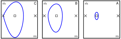
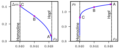
Figure 7: Line at fixed $c=1.12$ in the ($c$, $\rho_{g}$) space, for $c<c^{*}$. Top: Three phase portraits along the line, from the vicinity of the Hopf bifurcation line (A) until the homoclinic is found (C) Bottom-left: Size of the limit cycle $\Delta m$ defined in Eq. (28). The limit cycle disappears when $\Delta m$ is large enough that the orbit reaches $m=0$, where the trajectory is homoclinic. Bottom-right: Average density $\rho_{0}$ of the solutions. Parameters: $D=v_{0}=\lambda=\xi=a_{4}=\varphi_{g}=1$.

A symmetric behavior is observed when $c>c^{*}$, for the subcritical Hopf bifurcation. Increasing $\rho_{g}$, an unstable limit cycle of vanishing amplitude appears at $\rho_{g}=\rho_{g}^{H}$. The amplitude of the cycle then increases with $\rho_{g}$ until the trajectory hits the point $m=m_{+}$ where we have an (unstable) homoclinic solution that starts from $m=m_{+}$ as shown in Fig. 8. Physically, when increasing $\rho_{g}$, $m_{f}-m_{-}$ increases so that the friction around the stable fixed point at $m=m_{-}$ becomes larger and thus its basin of attraction (whose boundary is the unstable limit cycle, see Fig. 6) becomes larger.

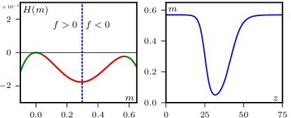
Figure 8: Unstable homoclinic trajectory starting from $m=m_{+}$ for $c=1.16$. Parameters: $D=v_{0}=\lambda=\xi=a_{4}=\varphi_{g}=1$.

All in all, the central results of this section is that all the admissible solutions lie in a band delimited by the Hopf bifurcation line $\rho_{g}^{H}(c)$ and a line where the homoclinic trajectories are found, as shown in Fig. 9. Inside this band there exists stable non-degenerate limit cycles, corresponding to periodic propagating profiles. The unique heteroclinic trajectory is located exactly at $c=c^{*}$ where the Hopf bifurcation changes from supercritical to subcritical. We thus observe a 2-parameter family of periodic solutions, a line of homoclinic trajectories and a unique heteroclinic trajectory. Going back to the original pattern formation problem, they correspond to a 2-parameter family of micro-phase separated profiles, a line of isolated solitonic bands and a unique phase-separated state where a macroscopic polar liquid domain cruises through a disordered gas.

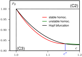
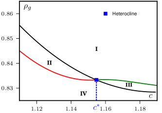
Figure 9: Space of all solutions. A 2-parameter family of periodic orbits is found inside the band delimited by the Hopf bifurcation and the homoclinic trajectories. The constraints (C2) and (C3) are indicated by the black dashed lines. The constraint (C1) lies out the range of this plot. Bottom: Zoom of the plot above around the point $c=c^{*}$ where the Hopf bifurcation changes from supercritical to subcritical. This is also where the unique heteroclinic trajectory is found. The roman numbers refer to Fig. 6, indicating the type of phase portrait found in each region. Parameters: $D=v_{0}=\lambda=\xi=a_{4}=\varphi_{g}=1$.

IV.6 Working at fixed average density

In the microscopic models and the original hydrodynamic equations the average density $\rho_{0}$ is a conserved quantity fixed by the initial condition. On the contrary, when considering the trajectories of the fictive particle $m(z)$, $\rho_{0}$ is not a priori fixed and varies between the different solutions. To compute the mean density on a trajectory $m(z)$ we simply average $\rho(z)=\rho_{g}+v_{0}m(z)/c$ over time.

As shown in Fig. 7 (bottom-right), we find that at fixed $c<c^{*}$, $\rho_{0}$ decreases when $\rho_{g}$ decreases. It ranges from $\rho_{0}=\rho_{g}+\frac{v_{0}}{c}m_{-}$ when $\rho_{g}=\rho_{g}^{H}$ to $\rho_{0}=\rho_{g}$ at the homoclinic trajectory where the portion of the trajectory with $m(z)\neq 0$ becomes negligibly small. Note that, at the heteroclinic trajectory, $\rho_{0}$ can take a large range of values. Since the size of the gas and liquid domains are arbitrary, the average density can take any value in $[\rho_{g}^{h},\rho_{\ell}^{h}]$ where $\rho_{g}^{h}$ and $\rho_{\ell}^{h}$ are the densities in the gas and liquid domains respectively.

Fixing $\rho_{0}$ adds a constraint that selects a line of solutions in the ($c$, $\rho_{g}$) space, as shown in Fig. 10 (left). For all $\rho_{0}\in[\rho_{g}^{h},\rho_{\ell}^{h}]$ these lines end at the heteroclinic trajectory. We also observe that, at fixed $\rho_{0}$, the closer the trajectories are to the heteroclinic solution, the larger their amplitude (see Fig. 10, right). This means that along a line $\rho_{0}=\text{cst}$, the higher the amplitude the faster the band excitations propagate. This point will turn out to be crucial when discussing the coarsening dynamics at the hydrodynamic level in Sec. VII.

Until now, we have shown that three different types of possible trajectories $m(z)$ exist, which correspond to all the propagative solutions observed in the microscopic models of flying spins. We have further identified the subset of values of the propagation speed $c$ and the gas density $\rho_{g}$ for which these solutions exist. We can now turn to the study of their dynamical stability at the hydrodynamic equation level. However, we first discuss analytically in the next section the shape of inhomogeneous solutions.

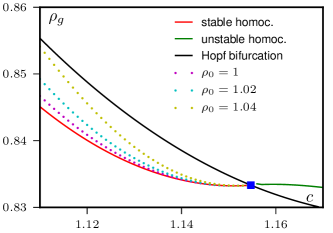
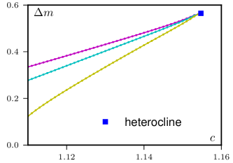
Figure 10: Top: Lines of solutions having a fixed average density $\rho_{0}$ in the space of all solutions. Bottom: the amplitude $\Delta m$ of the cycles, defined in Eq. (28), along the lines $\rho_{0}=\text{cst}$ increases when $c$ increases. Parameters: $D=v_{0}=\lambda=\xi=a_{4}=\varphi_{g}=1$.

IV.7 Exact solution for the heterocline

There are no general analytic solutions for the propagating inhomogeneous profiles. However, progress is possible for some limiting cases. In the following we show that a complete solution for the heterocline – its position in the ($c$, $\rho_{g}$) plane and its shape – can be determined exactly AIM . In A, we then show that, although exact solutions are not available, progress regarding the shape of the homoclinic solutions is achievable in the small $D$ limit.

To compute the shape of the heterocline, let us start from the ansatz

$$m_{1,2}(z)=\frac{m_{\ell}}{2}\Big{[}1+\tanh\big{(}k_{1,2}(z-z_{1,2})\big{)}\Big{]}$$ (29)

Each of $m_{1}(z)$ and $m_{2}(z)$ describe an interface centered around $z=z_{1,2}$ between a disordered phase with $m=0$ and an ordered phase with $m=m_{\ell}$. The complete heteroclinic trajectory then consists of two fronts glued together: An ascending front $m_{1}(z)$ with $k_{1}>0$ and a descending front $m_{2}(z)$ with $k_{2}<0$, with $z_{2}\gg z_{1}$ (see Fig. 11); Being part of the same profile, the two fronts share the same celerity $c$ and density $\rho_{g}$.

Moreover we know that $m_{\ell}$ must be located at the second maximum of $H$ so that

$$m_{\ell}=m_{+}=\frac{v_{0}}{2a_{4}c}\left(1+\sqrt{1-\frac{4a_{4}(\varphi_{g}-\rho_{g})c^{2}}{v_{0}^{2}}}\right)$$ (30)

Plugging $m_{1}$ and $m_{2}$ in Eq. (13) and replacing $m_{\ell}$ by its expression, one obtains for each of the fronts

$$g(c,\rho_{g},k_{1,2})+h(c,\rho_{g},k_{1,2})\tanh\left(k_{1,2}(z-z_{1,2})\right)=0$$ (31)

where $g$ and $h$ are complicated functions that we omit for conciseness. Eq. (31) can be true only if $g$ and $h$ vanish independently, for both $k_{1}$ and $k_{2}$.

We can express $k_{1}$ and $k_{2}$ as functions of $c$ and $\rho_{g}$ by linearizing the ansatz (29) around $m=0$. When $k_{1,2}(z-z_{1,2})\to-\infty$, one has $m_{1,2}\sim\exp(2k_{1,2}(z-z_{1,2}))$ so that we can identify $k_{1,2}$ with the two eigenvalues of the linear stability analysis Eq. (22). The ascending front is associated with the unstable direction $k_{1}=\lambda_{1}/2$ and the descending front with the stable direction $k_{2}=\lambda_{2}/2$.

Replacing $k_{1,2}$ by their values in Eq. (31), we have four equations for the two unknowns $c$ and $\rho_{g}$. After some algebra, one obtains a unique solution ($c^{h}$, $\rho_{g}^{h}$) with

$$c^{h} =c^{*}=\frac{\sqrt{v_{0}(3a_{4}\lambda+\xi)}}{\sqrt{3a_{4}}}$$ (32)

$$\rho_{g}^{h} =\varphi_{g}-\frac{2v_{0}}{9a_{4}\lambda+3\xi}$$ (33)

This gives us the magnetization $m_{\ell}$ and the the fronts steepness $k_{1,2}$ as

$$m_{\ell} =\frac{2v_{0}}{\sqrt{3a_{4}v_{0}(3a_{4}\lambda+\xi)}}$$ (34)

$$k_{1} =\frac{\sqrt{v_{0}(8a_{4}D+\xi^{2})}-\sqrt{v_{0}}\xi}{4D\sqrt{3a_{4}(3a_{4}\lambda+\xi)}}$$ (35)

$$k_{2} =\frac{-\sqrt{v_{0}(8a_{4}D+\xi^{2})}-\sqrt{v_{0}}\xi}{4D\sqrt{3a_{4}(3a_{4}\lambda+\xi)}}$$ (36)

In Fig. 11, we show that this solution matches exactly the heteroclinic orbit found by numerical integration of Eq. (20).

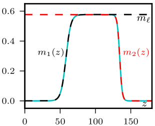
Figure 11: Comparison between the exact solution for the heterocline (dashed lines) and the result from numerical integration of Eq. (20) (blue line). Parameters: $D=v_{0}=\lambda=\xi=a_{4}=\varphi_{g}=1$.

V Back to the Vicsek-like and the active Ising models: non-linear solutions of the hydrodynamic equations

In Sec. III and IV we consider phenomenological hydrodynamic equations and assumed the simplest possible dependences of their coefficients with density. Here we extend our study to the more realistic hydrodynamic equations presented in Sec III.1. We first consider in Sec. V.1 the Vicsek hydrodynamic equations before turning to the Ising hydrodynamic equations in Sec. V.2. For sake of completeness, we also consider in Appendix B a more general case where the potential $H$ appearing in the dynamical system for $m(z)$ is not a polynomial in $m$. While not directly relevant for the hydrodynamic equations studied in this paper for the Vicsek and active Ising model, such Hamiltonians cannot be ruled out and may arise, for instance, from a density-dependence of the coefficient $a_{4}$ in the phenomenological hydrodynamic equations (8).

V.1 Vicsek like equations

Let us consider the hydrodynamic equations (3-III.1) introduced by Bertin and co-workers to describe a simplified version of the Vicsek model Bertin . These equations have the same structure as the phenomenological equations (7-8) with two additional gradient terms $\frac{\kappa}{2}\nabla(|\vec{m}|^{2})$ and $-\kappa(\nabla\cdot\vec{m})\vec{m}$. Importantly, all the coefficients $\gamma$, $\nu$, $\kappa$, $\mu$ and $\zeta$ depend on the density.

We follow the same approach as before. Looking for propagative solutions invariant in the transverse direction we set $m_{y}=0$, write $m_{x}=m$, and go to the comoving frame $z=x-ct$, to obtain

$$c \dot{\rho}-v_{0}\dot{m}=0$$ (37)

$$\nu\ddot{m} +\left(c-\frac{v_{0}^{2}}{2c}\right)\dot{m}-\gamma m\dot{m}-\frac{v_{0}}{2}\dot{\rho}+\mu m-\zeta m^{3}=0$$ (38)

Note that after setting $m_{y}=0$ the two $\kappa$ gradient terms of Eq. (III.1) cancel each other.

As before, Eq. (37) directly yields

$$\rho(z)=\rho_{g}+\frac{v_{0}}{c}m(z)$$ (39)

As we show in Appendix C, Eq. (38) can also be greatly simplified using the explicit density-dependence of its coefficients. Introducing $\tilde{\gamma}=\gamma/\nu$, $\tilde{\zeta}=\zeta/\nu$, and writing $\mu=\mu_{1}\rho-\mu_{2}$ and $\nu^{-1}=\nu_{1}\rho+\nu_{2}$, one obtains the second-order ordinary differential equation

$$\ddot{m}+(\alpha-\xi m)\dot{m}-a_{2}m+a_{3}m^{2}-a_{4}m^{3}=0$$ (40)

where the coefficients are all function of $c$ and $\rho_{g}$

$$\alpha =\left(c-\frac{v_{0}^{2}}{2c}\right)\left(\nu_{1}\rho_{g}+\nu_{2}\right)\qquad\xi=\frac{v_{0}^{3}}{2c^{2}}\nu_{1}+\tilde{\gamma}$$ (41)

$$a_{2} =\mu_{2}\nu_{2}+(\mu_{2}\nu_{1}-\mu_{1}\nu_{2})\rho_{g}-\mu_{1}\nu_{1}\rho_{g}^{2}$$

$$a_{3} =\frac{v_{0}}{c}\left(2\rho_{g}\mu_{1}\nu_{1}+\mu_{1}\nu_{2}-\mu_{2}\nu_{1}\right)$$

$$a_{4} =\tilde{\zeta}-\frac{v_{0}^{2}}{c^{2}}\mu_{1}\nu_{1}$$

Interestingly, Eq. (40) has exactly the same form as Eq. (13)—the dynamical system stemming from the phenomenological hydrodynamic equations studied in Sec IV—although with coefficients depending in a more complicated way on $\rho_{g}$ and $c$. Their propagative solutions will thus be the same, up to a slightly different organisation in the $c,\rho_{g}$ plane.

However, an important difference between the Vicsek and phenomenological hydrodynamic equations, is the scaling of the magnetization with density in the ordered phase. The Vicsek hydrodynamic equations (3-III.1) of Bertin and co-workers indeed predict that the homogeneous ordered solution satisfies

$$\frac{|\vec{m}_{0}|}{\rho_{0}}=\frac{1}{\rho_{0}}\sqrt{\frac{\mu}{\zeta}}\xrightarrow[\rho_{0}\to\infty]{}\sqrt{\frac{\mu_{1}\nu_{1}}{\tilde{\zeta}}}$$ (42)

which is consistent with what is observed in microscopic models such as the Vicsek model. On the contrary, because the coefficient $a_{4}$ in Eq. (8) does not depend on density, the phenomenological equations (7-8) would yield $\frac{m_{0}}{\rho_{0}}\to 0$ as $\rho_{0}$ increases. In this region of parameter space, which is not the main focus of this paper, the Vicsek hydrodynamic equations are thus more faithful to the phenomenology of microscopic models studied in Sec. II than the phenomenological equations (7-8). As we show in Appendix B, however, these phenomenological equations can recover a scaling akin to that of the Vicsek model if the coefficient $a_{4}$ of Eq. (8) is allowed to depend on density. This leads to a slightly more complicated dynamical system Caussin that we study in the appendix for completeness.

Coming back to the dynamical system (40), following the same method as that introduced in Sec. IV, one can derive analytical expressions for the Hopf bifurcation line $\rho_{g}^{H}(c)$ and the speed $c^{*}$ where the bifurcation becomes subcritical. We show in Fig. 12 the phase diagram in the ($c$, $\rho_{g}$)-plane and examples for the three types of inhomogeneous trajectories. Again an exact solution for the heteroclinic trajectory can be derived and (the dashed lines in Fig. 12) is found at speed $c^{h}=c^{*}$. As expected, there is no qualitative difference with the simpler case studied in Sec. III.

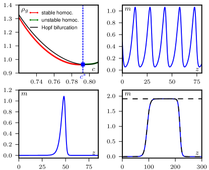
Figure 12: Top left: Phase diagram for the propagative solutions of the hydrodynamic equations of Bertin et al. Eq. (40). The color code and different phases are the same as for the $a_{4}=\text{cst}$ case Fig. 9. We obtain the same three types of inhomogeneous profiles: periodic, homoclinic and heteroclinic. $\sigma=0.7$.

V.2 Active Ising model equations

The active-Ising hydrodynamic equations AIM seem a priori different since they contain none of the non-linear gradient terms found in the phenomenological and Vicsek hydrodynamic equations. However, these terms are in fact generated by the diffusion term in the dynamical equation (5) for the density field AIM , so that we will once again recover the same types of propagative solutions.

Looking for stationary profiles in the comoving frame $z=x-ct$, Eq. (5) and (6) reduce to

$$D \ddot{\rho}+c\dot{\rho}-v_{0}\dot{m}=0$$ (43)

$$D \ddot{m}+c\dot{m}-v_{0}\dot{\rho}+2\left(\beta{}-1-\frac{r}{\rho}\right)m-\alpha\frac{m^{3}}{\rho^{2}}=0$$ (44)

Equation (43) can be solved by expanding $\rho$ in gradients of $m$. Introducing the ansatz

$$\rho(z)=\rho_{g}+\sum_{k=0}^{\infty}\alpha_{k}\frac{d^{k}m}{dz^{k}}$$ (45)

into Eq. (43), and solving order by order, we get the following recursion relation

$$a_{0}=\frac{v_{0}}{c}\qquad a_{k+1}=-\frac{D}{c}a_{k}$$ (46)

from which we obtain

$$\rho(z)=\rho_{g}+\frac{v_{0}}{c}\sum_{k=0}^{\infty}\left(-\frac{D}{c}\right)^{k}\frac{d^{k}m}{dz^{k}}$$ (47)

In the following we retain only the first order terms in gradient:

$$\rho(z)=\rho_{g}+\frac{v_{0}}{c}m(z)-\frac{Dv_{0}}{c^{2}}\dot{m}(z)+\frac{D^{2}v_{0}}{c^{3}}\ddot{m}(z)$$ (48)

To simplify Eq. (44) we linearize around the density $\varphi_{g}=r/(\beta{}-1)$ where the disordered profile becomes linearly unstable. As shown in AIM , this is a good approximation when $\beta\gtrsim 1$ because $\varphi_{g}\to\infty$ while $\rho-\varphi_{g}$ remains finite for inhomogeneous solutions. We then obtain

$$D\ddot{m}+c\dot{m}-v_{0}\dot{\rho}+\frac{2r}{\varphi_{g}^{2}}(\rho-\varphi_{g})m-\alpha\frac{m^{3}}{\varphi_{g}^{2}}=0$$ (49)

Finally, inserting Eq. (48) in the previous equation we obtain a second-order ordinary differential equation with exactly the same terms as those obtained from the phenomenological and Vicsek hydrodynamic equations, Eq. (13) and (40):

$$\tilde{D}\ddot{m}+\left(c-\frac{v_{0}^{2}}{c}-\xi m\right)\dot{m}-a_{2}m+a_{3}m^{2}-a_{4}m^{3}=0$$ (50)

with

$$\tilde{D}=D\left(1+\frac{v_{0}^{2}}{c^{2}}\right)\qquad\xi=\frac{4rDv_{0}}{(c^{2}+v_{0}^{2})\varphi_{g}^{2}}$$ (51)

$$a_{2}=\frac{2r(\varphi_{g}-\rho_{g})}{\varphi_{g}^{2}}\qquad a_{3}=\frac{2rv_{0}}{c\rho_{g}^{2}}\qquad a_{4}=\frac{\alpha}{\rho_{g}^{2}}$$ (52)

This equation has again the same qualitative behavior as in the phenomenological theory and the same three types of inhomogeneous solutions are found with the same organization in the ($c$, $\rho_{g}$) parameter space.

VI Linear stability of the propagative solutions in the 1D hydrodynamic equations

In sections IV and V, we have found and classified all the propagative solutions of different hydrodynamic equations. We have shown that in all cases three types of such solutions exist: periodic patterns of finite-size bands, solitary band solutions, and phase-separated solutions. These solutions were found as stable limit cycles, homoclinic, and heteroclinic orbits $m(z)$ of the reduced dynamical system (13). This study does not tell us anything about the local and a fortiori global stability of these solutions as solutions $m(x-ct)$ and $\rho(x-ct)$ of the original hydrodynamic partial differential equations. Indeed, a stable orbit of the reduced dynamical system can very well be unstable to spatiotemporal perturbations when re-expressed as an inhomogeneous propagative solution of the hydrodynamic equations. For example, consider the fixed point at $m=m_{-}$ which is stable for $\rho_{g}>\rho_{g}^{H}$, in the region I and III in Fig. 9. Without performing any calculation, we know that the corresponding homogeneous solution ($\rho_{0}=\rho_{g}+\frac{v_{0}}{c}m_{-}$, $m_{0}=m_{-}$) is unstable in the hydrodynamic equations because it lies inside the spinodal region where no homogeneous solution is linearly stable.

In this section we study the linear (local) stability of these solutions at the hydrodynamic level. Although, it is a well-defined linear problem, determining the stability of inhomogeneous solutions of nonlinear partial differential equations cannot be done analytically even in the (rare) cases where these solutions are known analytically. A direct numerical study is possible (for an example, see, e.g. NBSTAB ), but is rather tedious, all the more so as we deal with 2D hydrodynamic equations. In the following, we study mostly the linear stability of the hydrodynamic equations reduced to one dimension (that of propagation), using a simple numerical procedure explained below. For an account of some fully 2D preliminary investigation, see the end of this section.

VI.1 Numerical procedure

We investigated numerically the stability of the propagative solutions of the phenomenological hydrodynamic equations Eq. (7-8) reduced to one space dimension, that of propagation. To do so, we select a solution of the corresponding classical mechanics problem. (13) and use it as initial condition of the numerical integration of Eqs. (7) and (8).

The numerical integration is done using a semi-spectral algorithm, the linear terms being computed in Fourier space, the non-linear ones in real space and a semi-implicit time-stepping. This method, where the fields $\rho$ and $m$ are represented by their $N$ first Fourier modes (with $N$ large enough that the simulation has converged), is well suited to simulate systems with diffusion terms and periodic boundary conditions.

Preparing the initial condition of the hydrodynamic equations always brings in discretization errors. Indeed, because of the periodic boundary conditions in the hydrodynamic equations, we need to select a portion of the solution $m(z)$ which is a multiple of the period. This is done with an error of order $dx$, the space discretization step used in the numerical integration of (7) and (8).

Accordingly, we observe a rapid relaxation at short times due to the discretization errors. Subsequently, we find that the original solution is either stable at long times or is quickly destabilized and converges to another solution. To analyze systematically the stability of the propagative solutions, we defined a quantitative criterion for the stability: We choose a time $T_{s}=2000$ much larger than the relaxation time of the initial perturbation (which happens in a time $\sim 100$) but not too large to test solely the linear stability regardless of a possible long-time coarsening dynamics that could be induced by numerical noise. We then measure the amplitude of the solution $|\Delta m|(t)$ defined in Eq. (28) as a function of time. If

$$\delta m(T_{s})\equiv|\Delta m(T_{s})-\Delta m(0)|$$ (53)

is smaller than $10^{-3}$, the solution is said to be stable and unstable otherwise (see Fig. 13). This protocol does not give exact answers to the question of linear stability, since in particular the small but finite initial perturbations may take the initial condition out of the basin of attraction of a (stable) solution. But the results presented below are relatively robust to changing our numerical resolution and the conditions used to decide stability, and we are thus confident that they represent well the ’true’ subset of linear stable solutions.

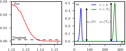
Figure 13: Stability of homoclinic orbits in the hydrodynamic equations. $\Delta a_{c}$ is the difference in the amplitude of the solution measured between $t=0$ and $t=T_{s}$. The solution is declared to be linearly stable if $\delta m(T_{s})$, defined in Eq. (53) is smaller than a threshold that we take at $10^{-3}$. $v_{0}=\lambda=\xi=a_{4}=\varphi_{g}=1$, $c=1.125$ (right)

The precise criterion does not matter much for the results since we find an abrupt transition from stable to unstable trajectories (see Fig. 13) which is visible on a variety of observables (norm of the fields, period, max and min values, etc).

VI.2 Results

Figure 14 contains one of the central results of our paper: only a very small subset of the propagative solutions are stable at the hydrodynamic level. However this subset includes the three possible types of trajectories: periodic bands, solitonic bands, and phase-separated profiles. The linearly stable solutions are all found in the region of the ($c$, $\rho_{g}$) plane close to the heteroclinic trajectory and close to the line of homoclinic orbits. Examples of stable and unstable solutions are shown in Fig. 15.

To understand why only the vicinity of the heteroclinic and homoclinic solutions is stable, one can argue that the solutions must have a large enough amplitude to be dynamically stable. Indeed, the periodic solutions oscillate around $m=m_{-}$ which lies inside the spinodal region of the hydrodynamic equations, where no homogeneous solutions is stable. Small-amplitude oscillations around this point should thus also by dynamically unstable and only large enough amplitude cycles, found near the homoclinic line and the heteroclinic trajectories, are stable.

Note that the region where stable solutions are found has a rather rough boundary in Fig. 14. This is most probably an artefact due to the initial discretization error which is not controlled and varies from one propagative solution to another. Close to the threshold of linear instability, this can easily make a (linearly) stable trajectory unstable.

We report finally on fully 2D simulations performed on rectangular boxes of width $L_{y}=100$, with small noise added to each grid point on a 1D solution extended trivially along $y$. These yielded essentially no change with respect to the results presented above. While this encourages us to believe that no unstable mode has components along $y$, and thus that the subset determined above corresponds to the linearly stable solutions of the full 2D hydrodynamic equations, we remain cautious. As a matter of fact, recent results obtained in the case of hydrodynamic equations for active nematics have revealed the existence of (very) long wavelength instability along the homogeneous direction of band solutions. NEMATIC A similar investigation is left for future studies.

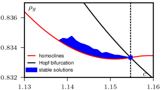
Figure 14: The blue region is the subset of admissible propagative solutions which are linearly stable. None of the solutions for $c>c^{*}$ is stable in the hydrodynamic equations. $v_{0}=\lambda=\xi=a_{4}=\varphi_{g}=1$. We use system sizes $L_{x}=300$ or more (adapted to fit the solution) with resolution $dx=0.5$ and $dt=0.1$.

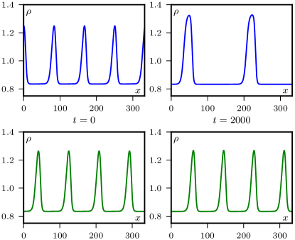
Figure 15: Evolution of two propagative solutions in the hydrodynamic equations  (7-8). The initial conditions are stable limit cycles of the dynamical system (13) for $m(z)$. Top row: unstable solution with $c=1.135$, $\rho_{g}=0.8351$. Bottom row: stable solutions with $c=1.14$, $\rho_{g}=0.8341$. System size $340\times 100$, $dt=0.1$, $dx=0.4$. $v_{0}=\lambda=\xi=a_{4}=\varphi_{g}=1$.

VII Coarsening in the hydrodynamic equations

The two-dimensional subset of propagative solutions that are linearly stable still contains an infinity of solutions, including smectic patterns, solitary bands, and phase-separated profiles. We can thus wonder whether a single solution is selected in the hydrodynamic equation starting from a random initial condition.

One can obtain some insight into this question by studying the lines of propagative solutions having a given average density $\rho_{0}$, shown in Fig. 10. Indeed, $\rho_{0}$ is conserved in the hydrodynamic equations and any stable propagative solutions has to lie on such a line. As discussed earlier, the larger the amplitude of a solution, the faster the propagation. We can thus expect that if several travelling bands coexist, they will encounter and merge because of their different speeds. This will in turn increase the sizes of the surviving objects and hence their speed. This mechanism would naturally lead the system toward the heteroclinic solution, i.e., to the phase-separated state.

We checked this scenario by simulating the phenomenological hydrodynamic equations (7-8) with three different initial conditions, as shown in Fig. 16:

• We build an initial condition made of two homoclines glued together, both solutions of the differential equation (13) for different speed $c$ and inside the stability domain of Fig. 14. To avoid discontinuities we interpolate smoothly between the gas densities of the two solutions using a hyperbolic tangent function. We then observe that the two travelling bands get closer until, when close enough (though not in contact), the smaller one evaporates, its mass being transfered to the second band. The final solution is hence a single larger isolated band.

• Starting from a random ordered solution with constant $\rho$ and a magnetization $m$ fluctuating around $m_{0}\neq 0$, several bands form at short times that all go in the same direction. The system then coarsens because of the speed differences between the liquid droplets until only “phase-separated domains”, that all have the same speed, remain. In practice, because the band speeds can be very close, a final state with a single phase-separated profile may not be reached within the time-scales of our simulations and a precise study of this coarsening regime is beyond our numerical capacities.

• Starting from a disordered initial condition with $m(x)$ fluctuating around $0$ and a density inside the spinodal region, many domains of positive and negative magnetization form. These objects then encounter and merge yielding a rapid coalescence process. Because of the periodic boundary conditions, this process typically yields a single phase-separated state for the system sizes we considered. For larger systems, the coalescence process could result in a larger number of bands propagating in the same direction. We should then observe the same type of coarsening as in the second case discussed above.

At the level of hydrodynamic equations, the fact that larger ordered domains travel faster leads to a natural coarsening towards the phase-separated states. This coarsening relies both on a coalescence process and, when bands travelling in the same direction are close enough, on a ripening during which a smaller band evaporates and is “swallowed” by its larger neighbour.

Note that we studied the stability of propagative solutions and their coarsening process using the phenomenological hydrodynamic equations (7-8). While the precise results will depend on the set of hydrodynamic equations under study, our simulations of the Vicsek and Ising hydrodynamic equations, (3-III.1) and (5-6), did not suggest any qualitative difference. Their comprehensive investigation, which is beyond the scope of this paper, would nevertheless be interesting, especially to quantifiy the role played by the non-linearities in the vectorial hydrodynamic equations (III.1).

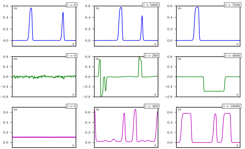
Figure 16: Coarsening in the phenomenological hydrodynamic equations (7-8) from three different initial conditions. Top: Two homoclinic trajectories glued together. Middle: Disordered initial condition. Bottom: Ordered initial condition. System size $500\times 100$ (top and bottom), $1000\times 100$ (middle). The profiles are averaged along the $y$-direction in which the system is invariant. $v_{0}=\lambda=\xi=a_{4}=\varphi_{g}=1$, $dt=0.1$, $dx=0.1$.

VIII Phase diagram of coarse-grained hydrodynamic equations

We can now construct the full phase diagram for the Ising and Vicsek hydrodynamic equations in the temperature-density ensemble (or noise-density for Vicsek), Fig. 17. It is composed of two spinodal lines, which are the limit of linear stability of the homogeneous disordered and ordered profiles, and two binodal lines outside which inhomogeneous solutions cannot be observed.

Figure 17: Phase diagram of the Visek (left) and Ising (right) hydrodynamic equations. The spinodal lines $\varphi_{g}$ and $\varphi_{\ell}$ are known exactly except $\varphi_{\ell}$ in the Vicsek hydrodynamic equation which we computed numerically by looking at the stability of systems of size $50\times 50$. The binodals $\rho_{g}$ and $\rho_{\ell}$ are the coexisting densities of phase-separated (heteroclinic) solutions as explained in the text. The dashed line indicate the asymptote above which only disordered solutions exist. Insets are close-ups on the high-density regions with a logarithmic scale on the $x$-axis. Parameters: $v_{0}=D=1=r=1$ (Ising), $v_{0}=1$ (Vicsek).

VIII.1 Spinodal lines

The spinodal lines can be determined analytically from a linear stability analysis, as was previously done for the Vicsek model Bertin and the active Ising model AIM . The lower spinodal line $\varphi_{g}$ is simply the density at which the coefficient of the term linear in $m$ in the hydrodynamic equations changes sign (in our phenomenological equation, when $a_{2}=0$). It reads for the Ising and Vicsek hydrodynamic equations

$$\varphi_{g}^{I}(T) =r/(\beta-1)$$ (54)

$$\varphi_{g}^{V}(\sigma) =\frac{\mu_{2}}{\mu_{1}}=\frac{\pi(1-e^{-\sigma^{2}/2})}{4(e^{-\sigma^{2}/2}-2/3)}$$ (55)

where $\beta=1/T$. The higher spinodal $\varphi_{\ell}$ can be determined exactly for the Ising hydrodynamic equations

$$\varphi_{\ell}^{I}(T)=\varphi_{g}\frac{v_{0}\sqrt{\alpha\left(v_{0}^{2}\kappa+8D(\beta-1)^{2}\right)}+v_{0}^{2}\kappa+8D\alpha(\beta-1)}{2v_{0}^{2}\kappa+8D\alpha(\beta-1)}$$ (56)

where $\kappa=2+\alpha-2\beta$ and $\alpha=\beta^{2}(1-\beta/3)$. For the Vicsek hydrodynamic equation, the exact determination of $\varphi_{\ell}$ is much more cumbersome Bertin . In Fig. 17 we show the line $\varphi_{\ell}^{V}(\sigma)$ computed numerically by simulating the Vicsek hydrodynamic equations at different densities in the homogeneous ordered state and looking at the growth of a small perturbation.

VIII.2 Binodal lines

The binodal lines $\rho_{g}$ and $\rho_{\ell}$ are defined as the minimum and maximum global densities beyond which inhomogeneous propagative profiles cannot be observed in simulations of the hydrodynamic equations. As explained in Sec. IV.6, at the heteroclinic trajectory the size of the liquid and gas domains are arbitrary so that phase-separated solutions can have any density in the range $[\rho_{g}^{h},\rho_{\ell}^{h}]$. We find that, for all parameters we tested, $\rho_{\ell}^{h}=\rho_{\ell}$, i.e., no other stable solution has a larger density than the liquid domain of the heteroclinic solution.

The situation is more subtle for the lower binodal $\rho_{g}$. Depending on the external parameters, the line of homoclinic trajectories solution of the dynamical system is not always monotonous as a function of $c$. For example, in the Vicsek hydrodynamic equation it is not monotonous at low noise, as shown in Fig. 18. In this case the minimum density accessible to propagative solutions is the minimum of the homoclinic line. This solution need not be stable in the hydrodynamic equations so that one should repeat the stability analysis done in Sec. VI for each value of the noise to determine exactly the binodal line. For simplicity, the lower binodal of the Vicsek hydrodynamic equation shown in Fig. 17 is the gas density read from the phase-separated profile, which is true at high noise and a good approximation of $\rho_{g}$ at lower noise values.

For the Vicsek hydrodynamic equations, the coexisting densities of the heteroclinic trajectory are known exactly whereas in the Ising case they can be determined analytically only after linearizing Eq. (44) around $\rho=\varphi_{g}$. The binodal lines in the phase diagram of the Ising hydrodynamic equations shown in Fig. 17 are thus determined by integrating numerically the hydrodynamic equations and measuring the density of the liquid and gas domain of a phase-separated solution whereas we plot the analytical solution in the Vicsek case.

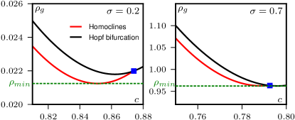
Figure 18: Propagative solutions of the Vicsek hydrodynamic equations for $\sigma=0.2$ and $0.7$. The solution with the lower mean density $\rho_{\text{min}}$ is found at the minimum of the line of homoclinic solutions. At low noise, it does not coincide with the heteroclinic solution (blue squares). $v_{0}=1$.

IX Conclusion

Before summarizing our results, let us discuss how the study of the hydrodynamic equations presented in this article compares with the phenomenology of the microscopic models. The phase diagrams of the Ising and Vicsek hydrodynamic equations shown in Fig. 17 are qualitatively similar. They are also consistent with the phase diagrams of the microscopic models shown in Fig. 2. The hydrodynamic equations thus provide a picture which is consistent with the liquid-gas framework discussed in Sec. II.3. For instance, the asymptote at finite noise (or temperature) can again be seen as the simplest way of forcing the system to cross a transition line to go from its gas to liquid phase.

The comparison between the phase-separated regions of the microscopic models and hydrodynamic equations is however more subtle. We have indeed shown, using the phenomenological hydrodynamic equation (7-8), that the coarsening leads, at the hydrodynamic level, to the phase-separated solution. This is true in the active Ising model but not in the Vicsek model, which only shows micro-phase separation and thus a coarsening leading to a periodic solution (see Fig. 1). This difference between microscopic models and hydrodynamic equations is however not surprising since it was recently shown that fluctuations are essential to account for the selection of micro-phase separated profiles in the Vicsek model Microphase .

More precisely, phase-separated and micro-phase-separated solutions are both linearly stable in the hydrodynamic equations for vectorial order parameters. As noise is added to these equations, though, large bands are destabilized and break in periodic array of finite-size bands, in agreement with what is seen in microscopic simuations of the Vicsek model Microphase . We can now tentatively put together these results to propose a coarsening process that would lead to the micro-phase separated states seen in the Vicsek model. Starting from a profile with many coexisting bands, the coarsening at fixed $\rho_{0}$ would tend to lead to the formation of larger and larger bands. This coarsening would however be arrested by the fact that the fluctuations in the Vicsek model set a maximal size beyond which bands are (non-linearly) unstable. How this size is selected however remains to be determined.

All in all, we have shown in this paper that the hydrodynamic equations describing polar flocking models generically share the same propagative solutions. We found three types of solutions that are all observed in microscopic models: periodic orbits that describe microphase separation, homoclinic orbits describing solitonic objects and heteroclinic trajectories that correspond to phase separation. Only a subset is stable in the hydrodynamic equations, but it still contains the three types of solutions.

The coarsening in the hydrodynamic equations favors the fastest solutions which are also the largest patterns. It thus leads naturally to the phase-separated solution which controls the phase diagram of the hydrodynamic equations. The same behavior is observed in the microscopic active Ising model whereas one can understand the microphase separation of the Vicsek model as an arrested coarsening, the largest pattern being non-linearly unstable to the (giant) fluctuations of the liquid phase.

Appendix A Limit of small $D$

While we do not have an analytic solution for the homoclinic profiles, lots of insight on their physics can be gained by studying the limit of small diffusion coefficient $D$. This is most easily done by introducing the auxiliary variable $Z=D\dot{m}+F(m)$ where

$$F(m)=\left(c-\frac{\lambda v_{0}}{c}\right)m-\frac{\xi}{2}m^{2}$$ (57)

such that $F^{\prime}(m)=f(m)$. Our dynamical system can then be recast as

$$\frac{d}{dz}\begin{pmatrix}m\\ Z\end{pmatrix}=\begin{pmatrix}\frac{1}{D}(Z-F(m))\\ -H^{\prime}(m)\end{pmatrix}$$ (58)

Let us consider a large-amplitude orbits that start close to $m=0$. An example of such orbits and the corresponding phase portrait for the ($m$, $Z$) variables is shown in Fig. 19. When $D$ is small, $\dot{m}$ relaxes quickly to zero so that $Z$ relaxes to the parabola $Z=F(m)$ in a time $\sim D$. Following the trajectory in Fig. 19, starting from point A at $m\approx 0$, the trajectory between A and B is above the parabola $F(m)$. The distance with the parabola first increases when $m<m_{-}$, which implies $H^{\prime}(m)<0$ and $\dot{Z}>0$, and decreases afterwards when $m>m_{-}$. The distance with the parabola stays of order $D$, set by the relaxation time of $\dot{m}$. When $Z=f(m)$ at point $B$, $m$ relaxes to $m=0$ in a time $\sim D$. This gives profiles with sharp leading fronts and long exponential tails, which are indeed consistent with the profiles seen at small temperature in the Vicsek model and its putative hydrodynamic description ChateGregoire ; Bertin ; Ihle .

This picture is consistent with the fact that at leading order in $D$ the eigenvalues at point ($m=0$, $\dot{m}=0$) read

$$\lambda_{1}=\frac{\varphi_{g}-\rho_{g}}{c-\lambda v_{0}/c}\qquad\lambda_{2}=-\frac{c-\lambda v_{0}/c}{D}$$ (59)

so that we have a slow unstable direction $\lambda_{1}$ and a fast stable direction $\lambda_{2}$. These two eigenvalues indeed control a large part of the trajectory, as shown in the right panel of Fig. 19.

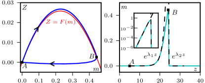
Figure 19: Left: Phase portrait for the variables $m$ and $Z=D\dot{m}+F(m)$ where $F(m)$ is the red parabola. Right: The corresponding trajectory. The dashed lines are the linear approximation around $m=0$. The inset in semi-log scale shows the exponential tail close to $m=0$. Parameters: $D=0.01$, $v_{0}=\lambda=\xi=a_{4}=\varphi_{g}=1$.

Appendix B Phenomenological equations with $a_{4}(\rho)$

In the hydrodynamic equation (8) the homogeneous ordered solutions have a magnetization $|\vec{m}_{0}|=\sqrt{a_{2}/a_{4}}$. Thus, in the simplified case studied in Sec. III where $a_{2}=\rho-\varphi_{g}$ and $a_{4}=\text{cst}$, one observes that

$$\frac{|\vec{m}_{0}|}{\rho}=\sqrt{\frac{\rho-\varphi_{g}}{a_{4}\rho^{2}}}\xrightarrow[\rho\to\infty]{}0$$ (60)

On the contrary we observe in the microscopic Vicsek and active Ising models that, at large densities, $|\vec{m}_{0}|/\rho_{0}$ reaches a constant $P_{0}\leq 1$ (set by the noise intensity in the microscopic models). This can be achieved by assuming that $a_{4}=(\rho P_{0}^{2})^{-1}$ as in Caussin so that

$$\frac{|\vec{m}_{0}|}{\rho}=P_{0}\sqrt{\frac{\rho-\varphi_{g}}{\rho}}\xrightarrow[\rho\to\infty]{}P_{0}$$ (61)

Repeating the same treatment as before, we look for 1d propagative solutions with speed $c$ which are the solutions of

$$D\ddot{m}+(c-\frac{\lambda v_{0}}{c}-\xi m)\dot{m}-(\varphi_{g}-\rho_{g})m\\ +\frac{v_{0}}{c}m^{2}-\frac{m^{3}}{P_{0}^{2}(\rho_{g}+\frac{v_{0}}{c}m)}=0$$ (62)

which can be written in the same form as Eq. (14) with a different potential

$$D\ddot{m} =-f(m)\dot{m}-H^{\prime}(m)$$ (63)

$$H(m) =-\frac{c^{3}\rho_{g}^{2}}{P_{0}^{2}v_{0}^{3}}m+\left[\frac{c^{2}\rho_{g}}{2P_{0}^{2}v_{0}^{2}}-\frac{(\varphi_{g}-\rho_{g})}{2}\right]m^{2}$$

$$-\left[\frac{c}{3P_{0}^{2}v}-\frac{v_{0}}{3c}\right]m^{3}+\frac{c^{4}\rho_{g}^{3}}{P_{0}^{2}v_{0}^{2}}\log(v_{0}m+c\rho_{g})$$ (64)

$$f(m) =c-\frac{\lambda v_{0}}{c}-\xi m$$ (65)

We find a behavior very similar to the case $a_{4}=\text{cst}$ discussed in section IV. Under the same constraints (C1-3), the potential $H(m)$ has the same form with maxima in $m=0$ and $m=m_{+}$ and a minimum at $m=m_{-}$ given by

$$m_{\pm}=\frac{cv_{0}P_{0}^{2}(2\rho_{g}-\varphi_{g})\pm cP_{0}\sqrt{(P_{0}v_{0}\varphi_{g})^{2}-4c^{2}\rho_{g}(\varphi_{g}-\rho_{g})}}{2(c^{2}-P_{0}^{2}v_{0}^{2})}$$ (66)

One observes the same three types of trajectories already shown in Fig. 5: periodic, homoclinic and heteroclinic. The phase diagram ($\rho_{g}$, $c$), shown in Fig. 20, is also similar to the case $a_{4}=\text{cst}$ except in a very small region close to the heteroclinic trajectory. We find again a 2-parameter family of periodic orbits and a line of homoclinic solutions which terminates at a unique heteroclinic trajectory.

As before, we can compute analytically the line $\rho_{g}^{H}(c)$ where the Hopf bifurcation takes place and the speed $c^{*}$ such that the bifurcation is supercritical for $c<c^{*}$ and subcritical for $c>c^{*}$. The difference with the previous case is that the heteroclinic trajectory, for which we do not have an exact solution anymore, is not found at $c=c^{*}$ but at $c^{h}>c^{*}$. As a consequence, we observe a new phase (shown as number V in Fig. 20) in which two limit cycles are found. A large stable cycle surrounds a smaller unstable limit cycle which itself encapsulates the stable fixed point $m=m_{-}$. As seen from the phase portraits in Fig. 20, when increasing $\rho_{g}$ the size of the stable cycle decreases whereas the size of the unstable one increases. Thus the upper limit of existence of this phase (the magenta line in the phase diagram) is the moment where the cycles collide and annihilate.

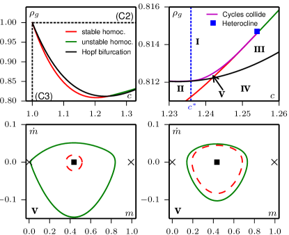
Figure 20: Top row: Phase diagram for the propagative solutions of Eq. (63). The right plot is a zoom on the region $c^{*}<c<c^{h}$. Phase I to IV are the same as in the case $a_{4}=\text{cst}$ (see Fig. 6). Bottom row: Phase portraits of the solutions in phase V for the same $c=1.2421$ and $\rho_{g}=0.81228$ (left) and $\rho_{g}=0.81248$ (right). When $\rho_{g}$ increases, the size of the stable cycle decreases while the size of the unstable cycle increases, until they collide as indicated on the phase diagram. $v_{0}=\lambda=\xi=P_{0}=\varphi_{g}=1$.

Appendix C Propagative solutions of the Vicsek hydrodynamic equations

Here we show how the study of propagative solutions in the Vicsek hydrodynamic equations leads to the same dynamical system as for the phenomenological equations, but with coefficients depending in a more complicated way on $\rho_{g}$ and $c$.

We start from the hydrodynamic equations (3-III.1) in the comoving frame $z=x-ct$:

$$c \dot{\rho}-v_{0}\dot{m}=0$$ (67)

$$\nu\ddot{m} +\left(c-\frac{v_{0}^{2}}{2c}\right)\dot{m}-\gamma m\dot{m}-\frac{v_{0}}{2}\dot{\rho}+\mu m-\zeta m^{3}=0$$ (68)

The coefficients in Eq. (68) are greatly simplified by dividing the equation by $\nu$, thus getting

$$\ddot{m}+\frac{1}{\nu}\left(c-\frac{v_{0}^{2}}{2c}\right)\dot{m}-\tilde{\gamma}m\dot{m}-\frac{v_{0}}{2\nu}\dot{\rho}+\frac{\mu}{\nu}m-\tilde{\zeta}m^{3}=0$$ (69)

where $\tilde{\gamma}=\gamma/\nu$ and $\tilde{\zeta}=\zeta/\nu$ depend only on the noise $\sigma$ on the alignment interaction Bertin

$$\tilde{\gamma} =\frac{8}{\pi}\left(\frac{16}{15}+2e^{-2\sigma^{2}}-e^{-\sigma^{2}/2}\right)$$ (70)

$$\tilde{\zeta} =\frac{64}{\pi^{2}}\left(e^{-\sigma^{2}/2}-\frac{2}{5}\right)\left(\frac{1}{3}+e^{-2\sigma^{2}}\right)$$ (71)

while $\mu$ and $\nu$ depend also on the density

$$\mu =\frac{4v_{0}\rho}{\pi}\left(e^{-\sigma^{2}/2}-\frac{2}{3}\right)-v_{0}\left(1-e^{-\sigma^{2}/2}\right)$$ (72)

$$\nu^{-1} =\frac{4}{v_{0}^{2}}\left[\frac{8\rho}{3\pi}\left(\frac{7}{5}+e^{-2\sigma^{2}}\right)+\left(1-e^{-2\sigma^{2}}\right)\right]$$ (73)

One can solve Eq. (67) to get $\rho(z)=\rho_{g}+\frac{v_{0}}{c}m(z)$ as before and use it in Eq. (69) to obtain the second-order ordinary differential equation

$$\ddot{m}+(\alpha-\xi m)\dot{m}-a_{2}m+a_{3}m^{2}-a_{4}m^{3}=0$$ (74)

where the coefficients are all function of $c$ and $\rho_{g}$

$$\alpha =\left(c-\frac{v_{0}^{2}}{2c}\right)\left(\nu_{1}\rho_{g}+\nu_{2}\right)\qquad\xi=\frac{v_{0}^{3}}{2c^{2}}\nu_{1}+\tilde{\gamma}$$ (75)

$$a_{2} =\mu_{2}\nu_{2}+(\mu_{2}\nu_{1}-\mu_{1}\nu_{2})\rho_{g}-\mu_{1}\nu_{1}\rho_{g}^{2}$$

$$a_{3} =\frac{v_{0}}{c}\left(2\rho_{g}\mu_{1}\nu_{1}+\mu_{1}\nu_{2}-\mu_{2}\nu_{1}\right)$$

$$a_{4} =\tilde{\zeta}-\frac{v_{0}^{2}}{c^{2}}\mu_{1}\nu_{1}$$

where $\mu_{1,2}$ are defined by $\mu=\mu_{1}\rho-\mu_{2}$ and $\nu_{1,2}$ by $\nu^{-1}=\nu_{1}\rho+\nu_{2}$.

References

- (1) Sepúlveda, N., Petitjean, L., Cochet, O., Grasland-Mongrain, E., Silberzan, P., Hakim, V. PLoS Comp. Biol., 9(3), e1002944 (2013)
- (2) F. Peruani, J. Starruss, V. Jakovljevic, L. Sogaard-Andersen, A. Deutsch, M. Bär, Phys. Rev. Lett. 108, 098102 (2012)
- (3) V. Schaller, C. Weber, C. Semmrich, E. Frey, A. R. Bausch, Nature 467, 73-77 (2010).
- (4) Y. Sumino, K. H. Nagai, Y. Shitaka, D. Tanaka, K. Yoshikawa, H. Chaté, K. Oiwa, Nature 483 448-452 (2012).
- (5) J. Deseigne, O. Dauchot, H. Chaté. Phys. Rev. Lett., 105, 098001 (2010); J. Deseigne, et al. Soft Matter 8, 5629 (2012); C.A. Weber, et al. Phys. Rev. Lett., 110, 208001 (2013).
- (6) A. Bricard, J.B. Caussin, N. Desreumaux, O. Dauchot, and D. Bartolo, Nature, 503, 95 (2013)
- (7) Shashi Thutupalli et al 2011 New J. Phys. 13 073021
- (8) T. Sanchez; D. T. N. Chen, S. J. DeCamp, M. Heymann, Z. Dogic, Nature 491 431 (2012).
- (9) T. Vicsek, A. Czirók, E. Ben-Jacob, I. Cohen, and O. Shochet, Phys. Rev. Lett. 75, 1226 (1995)
- (10) Mermin, N. D., Wagner, H. Phys. Rev. Lett. 17, 1133 (1966)
- (11) J. Toner, and Y. Tu, Phys. Rev. Lett. 75, 4326 (1995). J. Toner, Y. Tu, and M. Ulm, Phys. Rev. Lett. 80, 4819 (1998)
- (12) G. Grégoire, and H. Chaté, Phys. Rev. Lett. 92, 025702 (2004) ; H. Chaté, F. Ginelli, G. Grégoire, and F. Raynaud, Phys. Rev. E 77, 046113 (2008)
- (13) A.P. Solon, and J. Tailleur, Phys. Rev. Lett. 111, 078101 (2013)
- (14) A. P. Solon, H. Chaté, J. Tailleur, Phys. Rev. Lett. 114, 068101 (2015)
- (15) E. Bertin, M. Droz, G. Grégoire, Phys. Rev. E 74 022101 (2006); J. Phys. A 42 445001 (2009); A. Peshkov, E. Bertin, F. Ginelli and H. Chaté, Eur. Phys. J Special Topics 223, 1315 (2014).
- (16) J-B Caussin, A. Solon, A. Peshkov, H. Chaté, T. Dauxois, J. Tailleur, V. Vitelli, and D. Bartolo, Phys. Rev. Lett. 112, 148102 (2014)
- (17) S. Mishra, A. Baskaran, M.C. Marchetti. Phys. Rev. E 81, 061916. (2010); A. Gopinath, M.F. Hagan, M.C. Marchetti, A. Baskaran. Phys. Rev. E 85, 061903. (2012)
- (18) T. Ihle, Phys. Rev. E 83, 030901 (2011); T. Ihle, Phys. Rev. E 88, 040303(R) (2013).
- (19) F. D. C. Farrell, J. Tailleur, D. Marenduzzo, M. C. Marchetti, Phys. Rev. Lett. 108, 248101 (2012)
- (20) R. Großmann, L. Schimansky-Geier, and P. Romanczuk, New Journal of Physics 15, 085014 (2013)
- (21) Y. A. Kuznetsov, Elements of Applied Bifurcation Theory, Second Edition. Springer. (2004)
- (22) In the Vicsek model, the region in which solitary bands can be seen vanishes as the system size is taken to infinity. At fixed intensive parameters, doubling the system size indeed doubles the number of bands and increasing the system size hence asymptotically leads, in principle, to a smectic arrangements of bands.
- (23) Note that is actually a momemtum field in this context.
- (24) Again, in the infinite-size limit, the homoclinic orbits/solitary wave solutions are only observable in a codimension one subset of parameter space.
- (25) H. Chaté, and P. Manneville, Phys. Lett. A 171, 183 (1992).
- (26) S. Ngo, et al. Phys. Rev. Lett. 113, 038302 (2014).