Generation of maximally entangled states in hybrid two quantum dots mediated by a spherical metal nanoparticle driven by external laser field

Abstract

We theoretically study the generation of quantum correlations in a hybrid system composed by two interacting semiconductor quantum dots mediated by a metal nanoparticle and coupled to an external laser field. Interactions present in the hybrid system are treated using a semiclassical approximation except for the direct dipole-dipole interaction. We report the entanglement of formation, which gives information about entanglement quantum correlations, for continuous wave and pulsed driving applied fields. We have found that for proper values of the physical and geometrical parameters of the hybrid system the applied field can be tuned producing quantum correlations of significant value so that they can be useful in quantum information and computation processes.

1 Introduction

Generation of well-controlled quantum correlations is the main research of many scientists working in the relatively new field of quantum information and quantum processing [1]. The most thoroughly studied quantum correlation is the entanglement. This striking feature has been mainly quantified by means of the concurrence and the entanglement of formation (EoF) [2]. A prototype system, the simplest composite system which can display quantum entanglement, is a two-qubit system. Pairs of semiconductor quantum dots (SQDs) where each one is characterized by two-level states (ground state and excitonic excited state) are ideal experimentally realistic nanostructures. Moreover, by introducing a plasmonic nanostructure between the two SQDs, the local electromagnetic field can be altered in a somehow desirable way and strong quantum correlations can be obtained [3, 4, 5, 6, 7, 8, 9, 10, 11, 12, 13, 14, 15, 16, 17, 18, 19, 20, 21, 22, 23, 24, 25].

In the above area of studies, Artuso and Bryant [9] studied a system composed by two SQDs (modeled as two-level systems) mediated by a spherical metal nanoparticle (MNP). They gave emphasis to the interaction of the system with an external electromagnetic field and presented the population dynamics of the two-qubit system for several cases. Previously, He and Zhu [6] had studied the transient population dynamics and the entanglement dynamics of the same system in the absence of an external electromagnetic field. Also, quite recently, Nerkararyan and Bozhevolnyi [16] have investigated how the relaxation dynamics in a system of two quantum dipole emitters (modeled as three-level systems) coupled to a spherical MNP influences the entanglement dynamics.

The externally-driven coupled SQD — spherical MNP — SQD system [9] is a direct extension of the externally-driven coupled SQD — spherical MNP system, which is a basic system of quantum plasmonics [26]. In the externally-driven coupled SQD — spherical MNP system, the optical properties and the controlled population dynamics has been extensively studied [27, 28, 29, 30, 31, 32, 33, 34, 35, 36, 37, 38, 39, 40, 41]. In this work, we return to the externally-driven coupled SQD — spherical MNP — SQD system [9] and study in detail the entanglement between the two SQDs. We quantify the entanglement with the EoF and present results for both transient entanglement dynamics and the steady state value of entanglement for various system parameters.

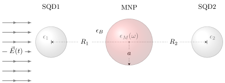
Figure 1: SQD — MNP — SQD geometry

This paper is organized as follows. In sect. 2, we present the theoretical model for the hybrid nanostructure in the presence of an applied external electromagnetic field and introduce a semi-classical scheme to describe the coupling of the pair of qubits directly to the applied field and through the MNP particle. While the direct SQD-SQD coupling is modeled quantum mechanically. Next, in sect. 3 we present the results for the time evolution of EoF and steady state results for EoF as a function of the various characteristic parameters of the hybrid system for both cw and pulsed fields. Finally, in sect. 4 we summarize our findings.

2 Theory

We consider a system as previously described in [9], where two identical SQDs (labeled by index $i(=1,2)$) mediated by a spherical metal nanoparticle of radius $\alpha$ are subject to a continuous sinusoidal wave (part 1) and pulsed laser (part 2) electric field (fig 1). The SQDs are at a center-to-center distance of $R_{i}$ from the MNP and the driving field of the applied cw is characterized by its magnitude $E_{0}$ and angular frequency $\omega$. For the pulsed laser field case, we assume a hyperbolic secant envelope, $f(t),E=E_{0}f(t)\cos(\omega t)$ with $f(t)=\textnormal{sech}\left((t-t_{0})/t_{p}\right)$, though the exact envelop shape is not of particular importance. The SQDs are directly coupled to the applied field, feel the electric field produced by the MNP and interact with each other.

We only consider two levels for the SQDs having exciton energies $\hbar\omega_{i}$, transition electric dipole moments $\mu_{i}$ and dielectric constants $\epsilon_{i}$. $\epsilon_{B}$ is the dielectric constant for the material in which the entire system is embedded.

The Hamiltonian for the system is

$$H_{\textnormal{t}otal}=H_{0}+H_{\textnormal{S}QD}+H_{\textnormal{i}nt}$$ (1)

where $H_{0}$ the unperturbed Hamiltonian, $H_{\textnormal{S}QD}$ describes the SQD — MNP interaction and $H_{\textnormal{i}nt}$ is the direct coupling between the SQDs.

We write $H_{0}$ as $H_{0}=\hbar\omega_{i}\hat{\alpha}_{i}^{\dagger}\alpha_{i}$, where repeated indexes imply summation over the indexes and $\hat{\alpha}^{(\dagger)}_{i}$ are the exciton annihilation (creation) operators for each SQD.

2.1 SQD — MNP interaction

We calculate $H_{\textnormal{S}QD}$ semi-classically, so $H_{\textnormal{S}QD}=-\mu_{i}(E_{SQDi}^{*}\hat{\alpha}_{i}^{\dagger}+E_{SQDi}\hat{\alpha}_{i})$. $E_{SQDi}$ is the electric field at the center of SQD$i$.

We write the electric field of the SQDs in terms of the screening factor ($\epsilon_{{\textnormal{eff}}i}=\frac{2\epsilon_{B}+\epsilon_{i}}{3\epsilon_{B}}$) and the induced field produced by the polarization of the MNP ($E_{M,i}$):

$$E_{SQDi}=\frac{1}{\epsilon_{{\textnormal{eff}}i}}(E(t)+E_{M,i})\,,$$

where the induced field and the polarization of the MNP are in turn [9]

$$E_{M,i} =\frac{1}{4\pi e_{B}}\frac{s_{\alpha}P_{\textnormal{MNP}}}{R_{i}^{3}}$$

$$P_{\textnormal{MNP}} =4\pi\gamma a^{3}e_{B}\left(E(t)+\frac{s_{\alpha}}{4\pi e_{B}}\sum_{i}\frac{P_{{\textnormal{SQD}}i}}{R_{i}^{3}\epsilon_{{\textnormal{eff}}i}}\right)$$

The polarization $P_{{\textnormal{SQD}}i}$ of each SQD is found from the density matrix elements, for the allowed transitions:

$$\frac{P_{{\textnormal{SQD}}i}}{\mu_{i}} =\ket{1}\rho\bra{\textnormal{SQD}i_{g}}+\ket{\textnormal{SQD}i_{g}}\rho\bra{1}+\ket{4}\rho\bra{\textnormal{SQD}i_{e}}+\ket{\textnormal{SQD}i_{e}}\rho\bra{4}$$

$$\frac{P_{{\textnormal{SQD}}1}}{\mu_{1}} =\rho_{1,2}+\rho_{2,1}+\rho_{4,3}+\rho_{3,4}$$

$$\frac{P_{{\textnormal{SQD}}2}}{\mu_{2}} =\rho_{1,3}+\rho_{3,1}+\rho_{4,2}+\rho_{2,4}$$

or, compactly, $\frac{P_{{\textnormal{SQD}}i}}{\mu_{i}}=\tilde{\rho}_{pi}+{\tilde{\rho}_{pi}}^{*}$, defining $\tilde{\rho}_{p1}=\rho_{1,2}+\rho_{3,4}$ and $\tilde{\rho}_{p2}=\rho_{1,3}+\rho_{2,4}$. Our basis is composed of four states, named $\ket{1}=\ket{g_{1}g_{2}}$, $\ket{2}=\ket{g_{1}e_{2}}$, $\ket{3}=\ket{e_{1}g_{2}}$ and $\ket{4}=\ket{e_{1}e_{2}}$, where $g_{i}$ and $e_{i}$ label the ground and the excited states of the $i$-qubit, respectively.

To simplify the expression for $P_{\textnormal{MNP}}$ we introduce the parameters $G_{i},\Omega_{i}$ and $F$:

$$G_{i} =\frac{\gamma\alpha^{3}s_{\alpha}^{2}\mu_{i}^{2}}{4\pi\epsilon_{B}\epsilon_{{\textnormal{eff}}i}^{2}R_{i}^{6}\hbar}$$

$$\Omega_{i} =\frac{E_{0}\mu_{i}}{2\hbar\epsilon_{{\textnormal{eff}}i}}(1+\frac{\gamma\alpha^{3}s_{\alpha}}{R_{i}^{3}})$$

$$F =\frac{1}{4\pi\epsilon_{B}}\frac{\gamma\alpha^{3}s_{\alpha}^{2}\mu_{1}\mu_{2}}{\hbar\epsilon_{{\textnormal{eff}}1}\epsilon_{{\textnormal{eff}}2}R_{1}^{3}R_{2}^{3}}$$

so we can now write:

$$E_{{\textnormal{S}QD}i} =\frac{G_{i}\hbar}{\mu_{i}^{2}}P_{{\textnormal{SQD}}i}+\frac{F\hbar}{\mu_{i}\mu_{\bar{\imath}}}P_{{\textnormal{SQD}}\bar{\imath}}+2f(t)\frac{\Omega_{i}\hbar}{\mu_{i}}\cos{\omega t}$$

$$H_{\textnormal{S}QD} =-\left(\frac{G_{i}\hbar}{\mu_{i}}P_{{\textnormal{SQD}}i}+\frac{F\hbar}{\mu_{\bar{\imath}}}P_{{\textnormal{SQD}}\bar{\imath}}+2f(t)\Omega_{i}\hbar\cos{\omega t}\right)\hat{\alpha}_{i}+\textnormal{h.c}$$ (2)

2.2 SQD direct coupling

For the direct coupling the Hamiltonian can be written [9, 42]

$$H_{\textnormal{i}nt}=\hbar\delta(\hat{\alpha}_{1}+\hat{\alpha}_{1}^{\dagger})(\hat{\alpha}_{2}+\hat{\alpha}_{2}^{\dagger})\,,$$ (3)

where $\delta$ is the interaction energy between the SQDs. In the model under study, all interaction fields are parallel to each other so we can write [8, 9, 42]

$$\delta(\omega,R_{1\leftrightarrow 2})=-\gamma_{\textnormal{e}m}\cdot\frac{3}{2}\left(\frac{\cos{\zeta}}{\zeta^{3}}+\frac{\sin{\zeta}}{\zeta^{2}}\right)$$

where $\zeta=\frac{\omega}{c}(R_{1}+R_{2})$ and $\gamma_{\textnormal{e}m}$ is the decay rate that characterizes the interaction.

In case we apply a semiclassical approximation for the direct coupling of the two quantum dots we report very different results that do not fully reveal the quantum mechanical nature of our system. However we have observed that the same (fully quantum treatment) is not necessary for the other interaction terms.

2.3 Rotating Wave Approximation and master equation

The final Hamiltonian is

$$H= \hbar\omega_{i}\hat{\alpha}_{i}^{\dagger}\alpha_{i}$$

$$-\hbar\alpha_{i}\cdot\left(2\Omega_{i}f(t)\cos{\omega t}+\frac{P_{{\textnormal{SQD}}i}}{\mu_{i}}G_{i}+\frac{P_{{\textnormal{SQD}}\bar{\imath}}}{\mu_{\bar{\imath}}}F\right)$$

$$-\hbar\alpha_{i}^{\dagger}\cdot\left(\textnormal{h.c.}\right)$$

$$+\hbar\delta(\hat{\alpha}_{1}+\hat{\alpha}_{1}^{\dagger})(\hat{\alpha}_{2}+\hat{\alpha}_{2}^{\dagger})\,,$$

We transform the Hamiltonian to a different basis:

$$\ket{1}\to e^{i\omega t}\ket{1},\ket{2}\to\ket{2},\ket{3}\to\ket{3},\ket{4}\to e^{-i\omega t}\ket{4}.$$

In this basis $P_{{\textnormal{SQD}}i}$ is

$$\frac{P_{{\textnormal{SQD}}i}}{\mu_{i}} =e^{i\omega t}\tilde{\rho}_{\textnormal{p}i}+e^{-i\omega t}\tilde{\rho}^{*}_{pi}$$

and the full Hamiltonian is, after a rotating wave approximation:

$$H_{\textnormal{t}otal}= \hbar(\omega_{i}-\omega)\hat{\alpha}_{i}^{\dagger}\alpha_{i}+\hbar\omega I_{4}$$

$$-\hbar\,\alpha_{i}\cdot\left(\Omega_{i}f(t)+G_{i}\tilde{\rho}_{pi}+F\tilde{\rho}_{p\bar{\imath}}\right)$$

$$-\hbar\,\alpha_{i}^{\dagger}\cdot\left(\textnormal{h.c}\right)$$

$$+\hbar\delta(\hat{\alpha}_{1}\cdot\hat{\alpha}_{2}^{\dagger})+\textnormal{h.c}$$

$$= -\hbar\begin{pmatrix}-\omega&H_{1}&H_{2}&0\\ H_{1}^{\star}&-\omega_{1}&0&H_{2}\\ {H_{2}}^{\star}&0&-\omega_{2}&H_{1}\\ 0&{H_{2}}^{\star}&{H_{1}}^{\star}&\omega-(\omega_{1}+\omega_{2})\end{pmatrix}+\hbar\begin{pmatrix}0&0&0&0\\ 0&0&\delta&0\\ 0&\delta&0&0\\ 0&0&0&0\end{pmatrix}$$ (4)

where $H_{1}=\Omega_{1}f(t)+G_{1}\tilde{\rho}_{p1}+F\tilde{\rho}_{p2}$ and $H_{2}=\Omega_{2}f(t)+G_{2}\tilde{\rho}_{p2}+F\tilde{\rho}_{p1}$

The master equation for the system is

$$\frac{d\rho}{dt}=\frac{i}{\hbar}[\rho,H]-\Gamma({\rho})\,,$$ (5)

where $\rho(t)$ is the density matrix of the system of the SQDs.

$\Gamma(\rho)$ is the relaxation matrix that describes the dissipative processes. We use the approximation by [9], treating the SQDs as non interacting. We calculate $\Gamma$ in terms of the density and relaxation matrices of each single SQD, The final relaxation matrix is given by

$$\Gamma(\rho)= \left(\frac{1}{T_{1}}(\mathbb{1}\otimes\sigma_{x})\circ\rho\right)+\left(\frac{1}{T_{2}}(\sigma_{x}\otimes\mathbb{1})\circ\rho\right)+$$

$$\left(-\frac{1}{\tau_{2}}(\sigma_{z}\otimes{[\rho]}_{34})\right)+\left(-\frac{1}{\tau_{1}}({[\rho]}_{24}\otimes\sigma_{z})\right)\,,$$

where $\mathbb{1}=\begin{pmatrix}1&1\\ 1&1\end{pmatrix}$, $\sigma_{i}$ the Pauli matrices, $\circ$ signifies pairwise product between matrices and ${[\rho]}_{ab}=\begin{pmatrix}\rho_{aa}&\rho_{ab}\\ \rho_{ba}&\rho_{bb}\end{pmatrix}$. The parameters $T_{i}$ and $\tau_{i}$ are relaxation times characteristic of the system: $\tau_{i}$ pertains to spontaneous decay of the exciton state, while $T_{i}$ pertains to decoherence by phonon interactions inside the SQD.

2.4 Entanglement measure

Finally, we present the measure of quantum correlations which is used in this work, i.e. the EoF. In order to find the EoF [2] we compute the matrix $R=\rho(t)(\sigma Ay\otimes\sigma By){\rho(t)}^{*}(\sigma Ay\otimes\sigma By)$, where $\rho(t)$ is the solution of the previous master equation and $\sigma iy$, with $i=A,B$ are the Pauli matrices of the two SQDs respectively. By diagonalising the matrix $R$, we compute its eigenvalues $\lambda_{j}$, with $j=1,2,3,4$, and then we calculate the concurrence, which is $C=\max[0,\sqrt{\lambda_{1}}-\sqrt{\lambda_{2}}-\sqrt{\lambda_{3}}-\sqrt{\lambda_{4}}]$ for $\lambda_{1}>\lambda_{2}>\lambda_{3}>\lambda_{4}$. Given that, we can compute the EoF expressed as

$$\textnormal{EoF}(\rho)=h(\frac{1+\sqrt{1-C^{2}(\rho)}}{2})\,,$$ (6)

where $h(x)=-x\log_{2}x-(1-x)\log_{2}(1-x)$ is the binary entropy function. The EoF takes values from 0 (no entanglement for the system) to 1 (maximum entanglement).

2.5 Parameters for the numerical calculations

We summarize the parameters $G_{i},F,\gamma,\Omega_{i},\delta$

$$G_{i} =\frac{\gamma\alpha^{3}s_{\alpha}^{2}\mu_{i}^{2}}{4\pi\epsilon_{B}\epsilon_{{\textnormal{eff}}i}^{2}R_{i}^{6}\hbar}$$

$$\Omega_{i} =\frac{E_{0}\mu_{i}}{2\hbar\epsilon_{{\textnormal{eff}}i}}(1+\frac{\gamma\alpha^{3}s_{\alpha}}{R_{i}^{3}})$$

$$F =\frac{1}{4\pi\epsilon_{B}}\frac{\gamma\alpha^{3}s_{\alpha}^{2}\mu_{1}\mu_{2}}{\hbar\epsilon_{{\textnormal{eff}}1}\epsilon_{{\textnormal{eff}}2}R_{1}^{3}R_{2}^{3}}$$

$$\delta =-\gamma_{\textnormal{e}m}\cdot\frac{6}{4}\left(\frac{\cos{\zeta}}{\zeta^{3}}+\frac{\sin{\zeta}}{\zeta^{2}}\right)$$

$$\zeta =\frac{\omega}{c}(R_{1}+R_{2})$$

$$\gamma =\frac{\epsilon_{M}(\omega)-\epsilon_{B}}{2\epsilon_{B}+\epsilon_{M}(\omega)}\,,$$

with $\epsilon_{M}(\omega)$ being the dielectric function of the MNP, which we consider as that of gold, found experimentally [43]. We set $\epsilon_{B}=\epsilon_{0}$ and $\epsilon_{1}=\epsilon_{2}=6\epsilon_{0}$ and use $\epsilon_{{\textnormal{eff}}i}=\frac{2\epsilon_{B}+\epsilon_{i}}{3\epsilon_{B}}$. We take $s_{\alpha}=2$ as all interaction fields are parallel to each other.

We set $\omega_{1}=\omega_{2}=$2.5\text{\,}\mathrm{e}\mathrm{V}$$, which is near the plasmon peak for gold (fig.2).

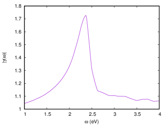
Figure 2: Experimentally found Dielectric response of gold [43]

For the radius of the MNP, $\alpha$, we use values in the range $0.1\text{\,}\mathrm{n}\mathrm{m}8\text{\,}\mathrm{n}\mathrm{m}$. We note that not all values in this range are practical but we use them nevertheless for completeness of the numerical analysis.

Also, we take $T_{1}=T_{2}=$0.3\text{\,}\mathrm{n}\mathrm{s}$$ and $\tau_{1}=\tau_{2}=$0.8\text{\,}\mathrm{n}\mathrm{s}$$. For $\gamma_{\textnormal{e}m}$ we use the geometric mean of the spontaneous decay rates of each SQD, $\gamma_{\textnormal{e}m}=\sqrt{1/T_{1}T_{2}}$

The characteristic times of the pulse are $t_{0}=$22.5\text{\,}\mathrm{p}\mathrm{s}$$ and $t_{p}=$3\text{\,}\mathrm{p}\mathrm{s}$$.

3 Results

In order to calculate the quantum correlations, we solve the set of differential equations of the density matrix elements of eq.5. We calculate the EoF which is a measure of the quantum correlations related to entanglement. In the present study our initial state is the most natural one, $\ket{1}=\ket{g_{1}g_{2}}$,, where both qubits are in the ground state. An external laser field is applied to the system. The intensity of the applied laser field is proportional to the square magnitude of $E_{0}$.

In fig. 3 we plot the time evolution of EoF for representative values of the geometric parameters of the hybrid system ($\alpha=$2\text{\,}\mathrm{n}\mathrm{m}$$, $\mu_{1}=\mu_{2}=$2.20\text{\,}\mathrm{e}\mathrm{n}\mathrm{m}$$ and $R_{1}=R_{2}=9$ nm). We apply a cw and pulsed laser field (of $t_{0}=$22.5\text{\,}\mathrm{p}\mathrm{s}$$ and $t_{p}=$3\text{\,}\mathrm{p}\mathrm{s}$$) with angular frequency of the field equals the excitonic transition eigenfrequency (resonance condition) and various characteristic intensities (for comparison and consistency see next figure, fig.4). First for the cw field we observe that EoF reaches a maximum value strongly depended on the magnitude of the applied field. For a value of 0.41 we get the maximum value (approximately 0.9). In all cases studied we have found that the maximum value is achieved at an early time and then the EoF performs an oscillatory decline, which is in accord o the characteristic relaxation times. Similarly, for the pulsed field the EoF reaches a maximum value of approximately 0.8 at the same intensity as in the cw case, and then smoothly declines. We emphasize here that we have observed this pattern in all cases that we investigated, for the same parameter set, the cw field achieves slightly higher EoF values that oscillate chaotically to lower values. Actually, two facts make the pulsed field more practical for use in quantum computation processes. First the gradual declination of EoF and second the observation that the maximum value of EoF can be related to the shape of the pulse (for example the peak position).

Then, in fig.4, we investigate the dependence of maximum EoF as a function of the intensity of the applied field for various angular frequencies of the field (on resonance and on off-resonance conditions). These are very informative plots and clearly reveal the importance of the intensity of the externally applied laser field on achieving high values of entanglement in a robust manner. A very significant observation is that in most cases investigated, above a characteristic value of the intensity the maximum EoF achieved has the same (relatively) high value. Moreover, in the off-resonance case there is a strong dependence on the position of the two SQDs (see the plot in the right column and middle row).

Then, we systematically study the dependence of EoF of the hybrid system on the various parameters of the system. In all cases studied we apply a cw and pulsed laser (of $t_{0}=$22.5\text{\,}\mathrm{p}\mathrm{s}$$ and $t_{p}=$3\text{\,}\mathrm{p}\mathrm{s}$$) with intensity, found under systematic numerical investigation, that maximizes the observed EoF. Hence, we mainly study maximum EoF as a function of the hybrid system geometrical parameters, i.e. size of MNP, dipole moments and the position of the SQDs, and the external parameters, i.e. the characteristic parameters of the external fields.

First, in fig. 5 we depict the density diagram of the maximum achieved EoF as a function of dipole moments of the two identical SQDs, $\mu_{1}=\mu_{2}$ and the radius of the MNP $\alpha$ for $R_{1}=R_{2}=9$ nm. From this diagram it appears that we have two distinct regions. One where we can find very high EoF values and a region of significantly lower EoF values. The observed behavior is in accordance to the one reported in top fig. 3 of ref. [9]. The region of high EoF corresponds to the EXIT and the transition chaotic region of the phase diagram there [9]. The transition suppression and the bistability region shows lower EoF. In the next figure (Fig. 6) we investigate the final EoF for the pulsed case, as the final EoF of the cw filed is always zero. We report that the shorter distance of $R_{1}=R_{2}=9$ nm case gives higher values of the EoF compared to the higher distance of $R_{1}=R_{2}=13$ nm case.

Finally, we have found a rather strong dependence of angular frequency of the laser field. In Fig. 7 we report for fixed radius of the MNP ($\alpha=1nm$) the maximum EoF as a function of the dipole moment of the SQDs and the detuning of the applied field and found a very strong dependence. Actually, fig. 7 is highly asymmetric, showing significant values of EoF only for negative detuning or for very close to resonance driving fields. We have found that for positive detuning, i.e. for incident photons of higher energy than the exciton energy, the EoF shows low values, strongly depending on the detuning

4 Summary

We have theoretically investigated the entanglement created in a hybrid nanostructure molecule consisting of two interacting SQDs coupled to a centrally located MNP driven by an external applied cw and pulsed laser field. The SQDs excitons are modeled quantum mechanically as two level systems and the MNP classically as a spherical MNP. Also, all interactions in the system are treated using a semiclassical approximation, except the direct SQDs coupling. The dynamics of the hybrid system is studied by means of the master equation of the density matrix of the two SQDs in the presence of the MNP. We use the density matrix elements and calculate the EoF numerically. In general, we have found that for proper values of the dipole moments of SQDs, the size of MNP and the distance of the SQDs from the MNP, as well as for the intensity of the applied, cw or pulsed field, we can produce steady state quantum correlations of significant value, and maximally entangled states so that they can be useful in quantum information and computation processes.

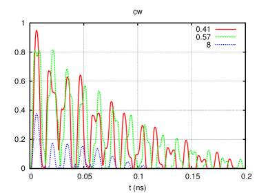
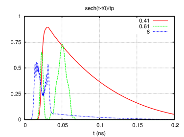
Figure 3: Plots of EoF as a function of time for a hybrid system on resonance. Radius of MNP is 2 nm, the dipole moment of each SQD is $2.20\text{\,}\mathrm{e}\mathrm{n}\mathrm{m}$ and the distance of each SQD from the MNP is $9\text{\,}\mathrm{n}\mathrm{m}$. Various plots are depicted for characteristic values for the intensity of the field ($1\text{\times}{10}^{6}\text{\,}\mathrm{V}\mathrm{/}\mathrm{m}$).

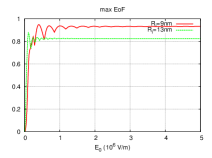
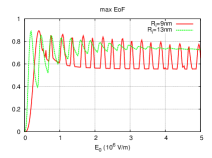
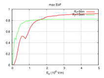
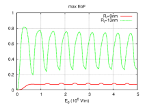
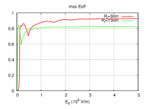
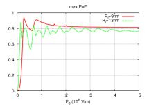
Figure 4: Plots of maximum EoF as a function of $E_{0}$ for a hybrid system on resonance (top), $\omega_{0}-\omega_{i}=-\delta$ (middle), $\omega_{0}-\omega_{i}=\delta$ (bottom). Radius of MNP is 2 nm, the dipole moment of each SQD is $2.20\text{\,}\mathrm{e}\mathrm{n}\mathrm{m}$ and the distance of each SQD from the MNP is $9\text{\,}\mathrm{n}\mathrm{m}$ (solid line) and $13\text{\,}\mathrm{n}\mathrm{m}$ (dashed). cw field (left) and secant pulse field (right).

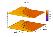
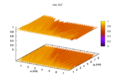
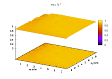
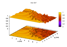
Figure 5: Dipole moment ($\mu_{1}=\mu_{2}$) vs. $\alpha$ phase diagram for maximum EoF achieved. cw field (top) and pulsed field (bottom). $R_{i}=$9\text{\,}\mathrm{n}\mathrm{m}$$ (left), $R_{i}=$13\text{\,}\mathrm{n}\mathrm{m}$$ (right). On the ($\mu$,$\alpha$) plane we depict the contour plot of the projection of the 3D picture.

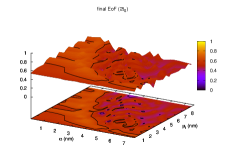
Figure 6: Comparison of maximum (see previous diagram) and final EoF for the dipole moment ($\mu_{1}=\mu_{2}$) vs. $\alpha$ phase diagram for the pulsed field. Final EoF is measured at $2t_{0}$. $R_{i}=$9\text{\,}\mathrm{n}\mathrm{m}$$ (left), $R_{i}=$13\text{\,}\mathrm{n}\mathrm{m}$$ (right).

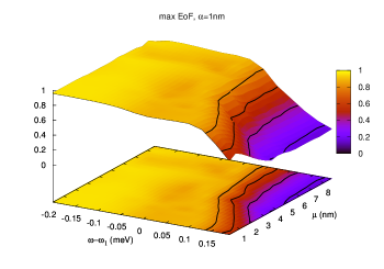
Figure 7: Dipole moment $\mu$ vs. detuning phase diagram for maximum EoF. The parameters are the same as in the previous phase diagram.

References

- [1] M.A. Nielsen and I.L. Chuang, Quantum Computation and Quantum Information (Cambridge University Press, Cambridge, 2000).
- [2] W. K. Wootters, Phys. Rev. Lett. 80, 2245 (1998).
- [3] A. Gonzalez-Tudela, D. Martin-Cano, E. Moreno, L. Martin-Moreno, C. Tejedor, and F. J. Garcia-Vidal, Phys. Rev. Lett. 106, 020501 (2011).
- [4] D. Martin-Cano, A. Gonzalez-Tudela, L. Martin-Moreno, F. J. Garcia-Vidal, C. Tejedor, and E. Moreno, Phys. Rev. B 84, 235306 (2011).
- [5] J. Xu, M. Al-Amri, Y. Yang, S.-Y. Zhu, and M. Suhail Zubairy, Phys. Rev. A 84, 032334 (2011).
- [6] Y. He and K.-D. Zhu, Nanosc. Res. Lett. 7, 95 (2012).
- [7] A. Gonzalez-Tudela, D. Martin-Cano, E. Moreno, L. Martin-Moreno, F. J. Garcia-Vidal, and C. Tejedor, Phys. Status Solidi C 9, 1303 (2012).
- [8] C. E. Susa, J. H. Reina, and L.L. Sanchez-Soto, J. Phys. B: At. Mol. Opt. Phys. 46, 224022 (2013).
- [9] R. D. Artuso and G. W. Bryant, Phys. Rev. B 87, 125423 (2013).
- [10] Q.-L. He, J.-B. Xu, and D.-X. Yao, Quant. Inf. Proc. 12, 3023 (2013).
- [11] S.-P. Liu, J.-H. Li, R. Yu, and Y. Wu, Phys. Rev. A 87, 042306 (2013).
- [12] C. Lee, M. Tame, C. Noh, J. Lim, S. A. Maier, J. Lee, and D. G. Angelakis, New J. Phys. 15, 083017 (2013).
- [13] C. E. Susa, J. H. Reina, and R. Hildner, Phys. Lett. A 378, 2371 (2014).
- [14] C. Racknor, M. R. Singh, Y. Zhang, D. J. S. Birch, and Y. Chen, Methods Appl. Fluoresc. 2, 015002 (2014).
- [15] J. Hou, K. Slowik, F. Lederer, and C. Rockstuhl Phys. Rev. B 89 235413 (2014).
- [16] K. V. Nerkararyan and S. I. Bozhevolnyi, Phys. Rev. B 92, 045410 (2015).
- [17] S. A. Hassani Gangaraj, A. Nemilentsau, G. W. Hanson, and S. Hughes, Optics Express 23, 22330 (2015).
- [18] Otten, Matthew and Shah, Raman A. and Scherer, Norbert F. and Min, Misun and Pelton, Matthew and Gray, Stephen K., Entanglement of two, three, or four plasmonically coupled quantum dots. Physical Review B 92, 125432 (2015).
- [19] Schindel, D. and Singh, M. R.., A study of energy absorption rate in a quantum dot and metallic nanosphere hybrid system. Journal of physics. Condensed matter 27, 345301 (2015).
- [20] Yang, Jianji and Perrin, Mathias and Lalanne, Philippe, Analytical Formalism for the Interaction of Two-Level Quantum Systems with Metal Nanoresonators. Physical Review X 5, 21008 (2015).
- [21] Nugroho, Bintoro S. and Malyshev, Victor A. and Knoester, Jasper, Tailoring optical response of a hybrid comprising a quantum dimer emitter strongly coupled to a metallic nanoparticle. Physical Review B 92, 165432 (2015).
- [22] Terzis, A. F. and Kosionis, S. G. and Boviatsis, J. and Paspalakis, E., Nonlinear optical susceptibilities of semiconductor quantum dot-metal nanoparticle hybrids. Journal of Modern Optics 63, 451 (2016).
- [23] Otten, Matthew and Larson, Jeffrey and Min, Misun and Wild, Stefan M. and Pelton, Matthew and Gray, Stephen, Origins and optimization of entanglement in plasmonically coupled quantum dots. Physical Review A 94, 022312 (2016).
- [24] Iliopoulos, Nikos and Terzis, Andreas F. and Yannopapas, Vassilios and Paspalakis, Emmanuel, Two-qubit correlations via a periodic plasmonic nanostructure. Annals of Physics 365, 38 (2016).
- [25] Sadeghi, Seyed M.; Mao, Chuanbin,Quantum sensing using coherent control of near-field polarization of quantum dot-metallic nanoparticle molecules. Journal of Applied Physics 121, 014309 (2017).
- [26] M. S. Tame, K. R. McEnery, S. K. Ozdemir, J. Lee, S. A. Maier, and M. S. Kim, Nature Physics 9, 329 (2013).
- [27] W. Zhang, A. O. Govorov, and G. W. Bryant, Phys. Rev. Lett. 97, 146804 (2006).
- [28] S. M. Sadeghi, Nanotechnology 20, 225401 (2009); Phys. Rev. B 79, 233309 (2009).
- [29] A. Ridolfo, O. Di Stefano, N. Fina, R. Saija, and S. Savasta, Phys. Rev. Lett. 105, 263601 (2010).
- [30] R. D. Artuso and G. W. Bryant, Phys. Rev. B 82, 195419 (2010).
- [31] A. V. Malyshev and V. A. Malyshev, Phys. Rev. B 84, 035314 (2011).
- [32] A. Hatef, D. G. Schindel, and M. R. Singh, Appl. Phys. Lett. 99, 181106 (2011).
- [33] S. G. Kosionis, A. F. Terzis, S. M. Sadeghi, and E. Paspalakis, J. Phys.: Condens. Matter 25, 045304 (2013).
- [34] E. Paspalakis, S. Evangelou, and A. F. Terzis, Phys. Rev. B 87, 235302 (2013).
- [35] A. Hatef, S. M. Sadeghi, S. Fortin-Deschênes, E. Boulais, and M. Meunier, Opt. Express 21, 5643 (2013).
- [36] B. S. Nugroho, A. A. Iskandar, V. A. Malyshev, and J. Knoester, J. Chem. Phys. 139, 014303 (2013).
- [37] M. E. Tasgin, Nanoscale 5, 8616 (2013).
- [38] S. M. Sadeghi, Phys. Rev. A 88, 013831 (2013).
- [39] M. A. Antón, F. Carreño, S. Melle, O. G. Calderón, E. Cabrera-Granado, and M. R. Singh, Phys. Rev. B 87, 195303 (2013).
- [40] J.-J. Li and K.-D. Zhu, Crit. Rev. Sol. State Mater. Sci. 39, 25 (2014).
- [41] Sadeghi, S. M., Dynamics of plasmonic field polarization induced by quantum coherence in quantum dot-metallic nanoshell structures. OPTICS LETTERS 39, 4986 (2014).
- [42] Lehmberg, R.H., Radiation from an N-atom system. I. General formalism. Physical Review A 2, 883 (1970).
- [43] B. Johnson and R. W. Christy, Phys. Rev. B 6, 4370 (1972).