Exact energy quantization condition for single Dirac particle in one- dimensional (scalar) potential well

Abstract

We present an exact quantization condition for the time independent solutions (energy eigenstates) of the one-dimensional Dirac equation with a scalar potential well characterized by only two ‘effective’ turning points (defined by the roots of $V(x)+mc^{2}=\pm E$) for a given energy $E$ and satisfying $mc^{2}+\min V(x)\geq 0$. This result generalizes the previously known non-relativistic quantization formula and preserves many physically desirable symmetries, besides attaining the correct non-relativistic limit. Numerical calculations demonstrate the utility of the formula for computing accurate energy eigenvalues.

I Introduction

In this paper we present a quantization formula for the one-dimensional Dirac equation using the analytical transfer matrix (ATM) method, thereby extending the non-relativistic analogue for the Schrödinger equation found by Cao et al. 1 ; 2 ; 3 . We focus on the relativistic energy levels offered by a simple confining scalar potential well with two turning points.

The high accuracy of the eigenvalues computable from this formula together with other applications like ground state reconstruction should prove to be useful in many applications of the Dirac equation, especially in the context of solid state physics 7 ; rev .

Our result can be thought of as a completion of well known semi-classical quantization formulae (like Bohr–Sommerfeld and WKB) in the following sense. The semi-classical quantization formulae provide reliable estimates of the energy eigenvalues only in the limit of large quantum numbers, while the ATM-quantization formula gives exact eigenvalues for all quantum numbers. As a result, Cao et al. additionally characterize this formula as an ‘exact quantization formula.’

In anticipation of the derivation given below, we would like to pursue this comparison a little further. The reader will recall that, in the WKB quantization formula, for instance, the boundary conditions at the turning points when applied to a suitably chosen approximate ansatz (for the actual wave function), lead to quantization of energy. However, the ATM method is based on transfer matrices which, in the appropriate limit ‘recovers’ the exact wave function $\Psi$ and the (corresponding) energy eigenvalue $E$. Structurally, the exact quantization formula contains the usual WKB term with a non-trivial correction contributed by the so-called ‘scattered sub- waves’, which is of great significance (discussed in Section II).

Particularly, for the Dirac equation the negative energy (antiparticle) solutions make the energy spectrum unbounded from below, which for general potentials is difficult to account for using the ATM method. Also, the generalization of this method for even the Schrödinger equation to potentials having more than two classical turning points ($x$ for which $V(x)=E$) is not clear at present. This difficulty translates to our inability to obtain the quantization condition for the Dirac problem for potential wells that either (1) give more than two classical turning points, or (2) satisfy $mc^{2}+\min V(x)<0$, or both. Owing to these limitations, we narrow our focus to potential wells with only two classical turning points and satisfying $mc^{2}+\min V(x)\geq 0$. For this restricted class of potential wells we can apply the ATM method successfully.

Following up with the derivation in Section II we point to some desirable symmetries of the quantization formula in Section III and discuss its non-relativistic limit. Section IV is devoted to numerical results and applications. We conclude in Section V outlining prospects of further study.

II Formulation

Consider the one-particle Dirac Hamiltonian $H=c\boldsymbol{\alpha}p+\boldsymbol{\beta}(mc^{2}+V)$, where $p=-i\hbar\mathrm{d}/\mathrm{d}x$ is the momentum operator and $m$ ($c$) is the rest mass of the particle (speed of light). We choose to represent the Dirac matrix $\boldsymbol{\alpha}(\boldsymbol{\beta})$ by the Pauli matrix $\boldsymbol{\sigma}_{y}(\boldsymbol{\sigma}_{z})$, which has the advantage that the two-component wave function $\Psi=\begin{pmatrix}\psi_{1}&\psi_{2}\end{pmatrix}^{\top}$ can be chosen to be real 4 ; 5 . The time independent Dirac equation prescribes the eigenvalue problem $H\Psi=E\Psi$, where $E$ is the energy of the particle. Further, the property $H\Psi^{\prime}=-E\Psi^{\prime}\Rightarrow\Psi^{\prime}=\boldsymbol{\sigma}_{x}\Psi$ shows that the positive and negative solutions occur in pairs. Hence, it suffices to consider positive energy solutions alone.

The (reduced) Compton wavelength $\hbar/mc$ and rest mass energy $mc^{2}$ provide natural length and energy scales in this problem. Thus, expressing every quantity in dimensionless form $x\rightarrow\hbar/mc\ \xi$, $E\rightarrow mc^{2}\varepsilon$, $V\rightarrow mc^{2}\vartheta$, the Dirac equation translates into the coupled first order system of equations

$$\dot{\psi}_{1}=(1+\vartheta(\xi)+\varepsilon)\psi_{2}$$ (1)

$$\dot{\psi}_{2}=(1+\vartheta(\xi)-\varepsilon)\psi_{1}$$ (2)

the overhead dot denoting differentiation w.r.t. $\xi$. We identify solutions of the equations $1+\vartheta(\xi)=\pm\varepsilon$ as effective turning points. For the schematic potential well depicted in Fig. 1, two turning points $\xi_{L,R}(\xi_{L}<\xi_{R})$ are obtained for a typical energy $\varepsilon$. Note that more than two effective turning points would result for $|\varepsilon|<-(1+\min\vartheta)$ unless the restrictions noted in Section I are enforced on $V$.

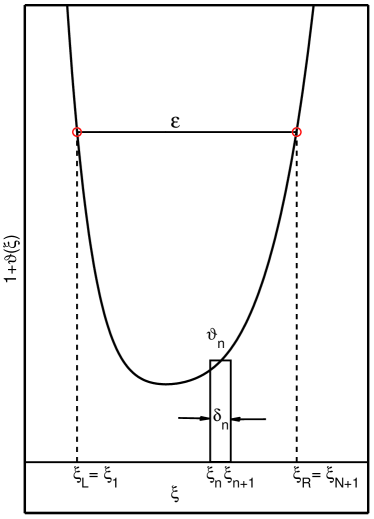
Figure 1: The (scalar) potential well $\vartheta(\xi)$, showing effective turning points $\xi_{L,R}$ for a typical energy $\varepsilon$.

Next, we partition the interval between the two turning points into $N$ segments $\xi_{L}=\xi_{1}<\xi_{2}\dotsm<\xi_{N}<\xi_{N+1}=\xi_{R}$. Denoting the width of the $n$^th segment by $\delta_{n}$, we choose an arbitrary point (a tag) $\xi^{\prime}_{n}$ within each segment and replace the scalar potential by a piecewise-constant approximation for which the potential in the $n$ ^th segment is given by $\vartheta_{n}=\vartheta(\xi^{\prime}_{n})$. Consequently, on this segment the system of Eqs. (1) and (2) admits a general solution of the form

$$\Psi^{n}=A_{n}\begin{pmatrix}1\\ {i\lambda_{n}}\end{pmatrix}e^{i\kappa_{n}(\xi-\xi_{n})}+B_{n}\begin{pmatrix}1\\ {-i\lambda_{n}}\end{pmatrix}e^{-i\kappa_{n}(\xi-\xi_{n})},$$ (3)

where $A_{n}$ and $B_{n}$ are arbitrary coefficients, and

$$\kappa_{n}=\sqrt{\varepsilon^{2}-(1+\vartheta_{n})^{2}},\ \lambda_{n}=\sqrt{\frac{\varepsilon-\vartheta_{n}-1}{\varepsilon+\vartheta_{n}+1}}.$$

Note that in the region of interest $\kappa_{n}$, $\lambda_{n}$ are real, hence the wave function components $\psi_{1,2}^{n}$ are oscillatory. In favor of a simpler notation, we drop the superscript $n$ from the wave function and infer the segment label from the context.

Ensuring the continuity of $\Psi^{n}$ at the ends of the segment leads to the ( transfer) matrix equation

$$\begin{pmatrix}\psi_{1}(\xi_{n})\\ \psi_{2}(\xi_{n})\end{pmatrix}=\begin{pmatrix}{\cos(\kappa_{n}\delta_{n})}&{-\frac{\sin(\kappa_{n}\delta_{n})}{\lambda_{n}}}\\ {\lambda_{n}\sin(\kappa_{n}\delta_{n})}&{\cos(\kappa_{n}\delta_{n})}\end{pmatrix}\begin{pmatrix}\psi_{1}(\xi_{n+1})\\ \psi_{2}(\xi_{n+1})\end{pmatrix}$$ (4)

Since we allow only two turning points at this stage, $\lambda_{n}$ is nonzero in each segment. Consequently, the transfer matrices are always well defined. Now, left multiplying Eq. (4) by $\begin{pmatrix}-\psi_{2}(\xi_{n})&\psi_{1}(\xi_{n})\end{pmatrix}$ and dividing the resulting equation by $\psi_{1}(\xi_{n})\psi_{1}(\xi_{n+1})$, we arrive at

$$\begin{pmatrix}P_{n}&1\end{pmatrix}\begin{pmatrix}{\cos(\kappa_{n}\delta_{n})}&{-\frac{\sin(\kappa_{n}\delta_{n})}{\lambda_{n}}}\\ {\lambda_{n}\sin(\kappa_{n}\delta_{n})}&{\cos(\kappa_{n}\delta_{n})}\end{pmatrix}\begin{pmatrix}1\\ -P_{n+1}\end{pmatrix}=0\\$$

where $P_{j}=-\psi_{2}(\xi_{j})/\psi_{1}(\xi_{j})$. Simplifying this matrix equation gives the recurrence formula

$$\frac{P_{n}}{\lambda_{n}}=\tan\bigg{(}\tan^{-1}\bigg{(}\frac{P_{n+1}}{\lambda_{n}}\bigg{)}-\kappa_{n}\delta_{n}\bigg{)},$$ (5)

$$\Rightarrow\tan^{-1}\bigg{(}\frac{P_{n}}{\lambda_{n}}\bigg{)}-\tan^{-1}\bigg{(}\frac{P_{n+1}}{\lambda_{n}}\bigg{)}=z\pi-\kappa_{n}\delta_{n},$$

$$\hskip 140.00021ptz=0,1,2,\ldots$$ (6)

Rearranging Eq. (6) and summing over $n$ from 1 to $N$ yields

$$\sum_{n=1}^{N}\kappa_{n}\delta_{n}+\sum_{n=1}^{N-1}\tan^{-1}\bigg{(}\frac{P_{n+1}}{\lambda_{n+1}}\bigg{)}-\tan^{-1}\bigg{(}\frac{P_{n+1}}{\lambda_{n}}\bigg{)}\\ =z\pi+\tan^{-1}\bigg{(}\frac{P_{N+1}}{\lambda_{N}}\bigg{)}-\tan^{-1}\bigg{(}\frac{P_{1}}{\lambda_{1}}\bigg{)}\ z=0,1,2,\ldots$$ (7)

The desired quantization condition emerges as a limit of Eq. (7) as $\delta(\mathrel{\hbox to0.0pt{\raisebox{1.29167pt}{$\cdot$}\hss}\raisebox{-1.29167pt}{$\cdot$}}=\max\delta_{n})\rightarrow 0$. In the limiting event, the continuous potential variation $\vartheta(\xi)$ is recovered, with $P_{1}\rightarrow P(\xi_{L})$ and $P_{N+1}\rightarrow P(\xi_{R})$. In Appendix A we prove that (for bound state wave functions) $P(\xi_{L})<0<P(\xi_{R})$ and $|P(\xi_{L,R})|<\infty$. Also, as $\delta\rightarrow 0$, $\lambda_{1,N}\rightarrow\lambda(\xi_{L,R})=0$. As a result, the ‘half phase losses’ at the effective turning points are given by

$$\lim_{\delta\rightarrow 0}\tan^{-1}\left(\frac{P_{N+1}}{\lambda_{N}}\right) =-\lim_{\delta\rightarrow 0}\tan^{-1}\left(\frac{P_{1}}{\lambda_{1}}\right)=\frac{\pi}{2},$$

$$\delta \mathrel{\hbox to0.0pt{\raisebox{1.29167pt}{$\cdot$}\hss}\raisebox{-1.29167pt}{$\cdot$}}=\max_{n}\delta_{n}.$$ (8)

Next, we account for the phase contribution of the so-called scattered sub- waves. Defining the phase contribution for each segment

$$\Delta\phi_{n} \mathrel{\hbox to0.0pt{\raisebox{1.29167pt}{$\cdot$}\hss}\raisebox{-1.29167pt}{$\cdot$}}=\tan^{-1}\left(\frac{P_{n+1}}{\lambda_{n+1}}\right)-\tan^{-1}\left(\frac{P_{n+1}}{\lambda_{n}}\right)$$

$$=\tan^{-1}\left(\frac{P_{n+1}\left(\lambda_{n}-\lambda_{n+1}\right)}{P^{2}_{n+1}+\lambda_{n}\lambda_{n+1}}\right)$$

$$=-\frac{P_{n+1}\left(\lambda_{n+1}-\lambda_{n}\right)}{P^{2}_{n+1}+\lambda_{n}\lambda_{n+1}}+\mathcal{O}\left(\left(\lambda_{n+1}-\lambda_{n}\right)^{3}\right),$$

which results from expanding the inverse tangent in a Taylor series in powers of $\left(\lambda_{n+1}-\lambda_{n}\right)$, we obtain the total phase contribution of the scattered sub-waves by

$$\lim_{\delta\rightarrow 0}\sum_{n=1}^{N-1}\Delta\phi_{n}=-\lim_{\delta\rightarrow 0}\sum_{n=1}^{N-1}\frac{P_{n+1}\left(\lambda_{n+1}-\lambda_{n}\right)}{P^{2}_{n+1}+\lambda_{n}\lambda_{n+1}}+\\ \lim_{\delta\rightarrow 0}\sum_{n=1}^{N-1}\mathcal{O}\left(\left(\lambda_{n+1}-\lambda_{n}\right)^{3}\right)=-\int_{\xi_{L}}^{\xi_{R}}\frac{P\dot{\lambda}}{P^{2}+\lambda^{2}}\mathrm{d}\xi$$ (9)

Thus, in the limit $\delta\rightarrow 0$, Eq. (7) takes the form

$$\int_{\xi_{L}}^{\xi_{R}}\kappa-\left(\frac{P\dot{\lambda}}{P^{2}+\lambda^{2}}\right)\mathrm{d}\xi=(z+1)\pi,\quad z=0,1,2...$$ (10)

We can phrase this result differently by substituting

$$\lambda^{2}=\frac{\varepsilon-\vartheta(\xi)-1}{\varepsilon+\vartheta(\xi)+1},\ P=-\frac{\psi_{2}}{\psi_{1}},$$ (11)

and using Eqs. (1) and (2), obtaining

$$\frac{P}{P^{2}+\lambda^{2}}\dot{\lambda}=\frac{\psi_{1}\psi_{2}(1+\vartheta(\xi)+\varepsilon)}{(1+\vartheta(\xi)+\varepsilon)\psi_{2}^{2}-(1+\vartheta(\xi)-\varepsilon)\psi_{1}^{2}}$$

$$\times\frac{-\varepsilon\dot{\vartheta}(\xi)}{\lambda(1+\vartheta(\xi)+\varepsilon)^{2}}=\frac{\varepsilon\dot{\vartheta}(\xi)}{\kappa}\left(\frac{\psi_{1}\psi_{2}}{\dot{\psi_{1}}\psi_{2}-\dot{\psi_{2}}\psi_{1}}\right)$$

$$=\frac{\varepsilon\dot{\vartheta}(\xi)}{2\kappa}\left(\frac{\Psi^{\dagger}\boldsymbol{\sigma}_{x}\Psi}{\Psi^{\dagger}\left(-i\boldsymbol{\sigma}_{y}\mathrm{d}/\mathrm{d}\xi\right)\Psi}\right)$$ (12)

$$=-\frac{\varepsilon\dot{\kappa}}{4i\sqrt{\varepsilon^{2}-\kappa^{2}}}\left(\frac{\Psi^{\dagger}[\boldsymbol{\sigma}_{y},\boldsymbol{\sigma}_{z}]\Psi}{\Psi^{\dagger}\left(-i\boldsymbol{\sigma}_{y}\mathrm{d}/\mathrm{d}\xi\right)\Psi}\right)$$

$$\hskip 110.00017pt\because\ 2i\boldsymbol{\sigma}_{x}=[\boldsymbol{\sigma}_{y},\boldsymbol{\sigma}_{z}].$$ (13)

Using this result and replacing the Pauli matrices with the Dirac matrices gives a representation independent form (Ref. Section III) of Eq. (10). Further, restoring the dimensions of the physical quantities and using $n$ (instead of $z$) for the quantum number yields

$$\int_{x_{L}}^{x_{R}}\frac{K}{\hbar c}+\bigg{(}\frac{E}{4\sqrt{K^{2}-E^{2}}}\frac{\mathrm{d}K}{\mathrm{d}x}\bigg{)}\bigg{(}\frac{\Psi^{\dagger}[\boldsymbol{\alpha},\boldsymbol{\beta}]\Psi}{\Psi^{\dagger}(c\boldsymbol{\alpha}p)\Psi}\bigg{)}\mathrm{d}x\\ =(n+1)\pi,\\ n=0,1,2,\ldots$$ (14)

where $K=\sqrt{E^{2}-(mc^{2}+V(x))^{2}}$, and the effective turning points satisfy $V(x_{L,R})+mc^{2}=\pm E$.

III Discussion

We begin by describing two symmetries of Eq. (14) that are physically desirable.

III.1 Representation independence

In Section II we chose a convenient representation of the Dirac matrices $\boldsymbol{\alpha}(\boldsymbol{\beta})=\boldsymbol{\sigma}_{y}(\boldsymbol{\sigma}_{z})$. However, the quantized energy levels are a property of the potential $V(x)$, hence should be independent of the chosen representation. This feature is already built into the quantization condition and can be shown in the following way. We know that the Dirac matrices satisfy the algebra: $\boldsymbol{\alpha}^{2}=\boldsymbol{\beta}^{2}=1\!\!1$ and $\{\boldsymbol{\alpha},\boldsymbol{\beta}\}=0$. Given any other representation of the Dirac matrices (denoted $\boldsymbol{\alpha}^{\prime},\boldsymbol{\beta}^{\prime}$) satisfying the same algebra, (a generalization of) Pauli’s fundamental theorem 6 asserts that there exists a unique (invertible) matrix $\boldsymbol{S}$ (up to a multiplicative complex constant) such that

$$\boldsymbol{\gamma}=\boldsymbol{S}^{-1}\boldsymbol{\gamma}^{\prime}\boldsymbol{S},\qquad\boldsymbol{\gamma}=\boldsymbol{\alpha},\boldsymbol{\beta}$$ (15)

A direct substitution shows that this transformation preserves the structure of the Dirac equation (for the same $E$) with the wave function transforming as $\Psi^{\prime}=\boldsymbol{S}\Psi$. Additionally, as the Dirac matrices are hermitian, we must have $\boldsymbol{S}^{\dagger}=\boldsymbol{S}^{-1}$ (unitarity of $\boldsymbol{S}$). Using the transformation Eq. (15) in Eq. (14) and noting that $[\boldsymbol{\alpha},\boldsymbol{\beta}]=\boldsymbol{S}^{\dagger}[\boldsymbol{\alpha}^{\prime},\boldsymbol{\beta}^{\prime}]\boldsymbol{S}$ gives

$$\frac{\Psi^{\dagger}[\boldsymbol{\alpha},\boldsymbol{\beta}]\Psi}{\Psi^{\dagger}(c\boldsymbol{\alpha}p)\Psi}\mapsto\frac{\Psi^{\prime\dagger}[\boldsymbol{\alpha^{\prime}},\boldsymbol{\beta^{\prime}}]\Psi^{\prime}}{\Psi^{\prime\dagger}(c\boldsymbol{\alpha^{\prime}}p)\Psi^{\prime}}$$

thus confirming the representation independence of the obtained quantization condition.

III.2 Symmetry w.r.t. the sign of $\boldsymbol{E}$

Although we assumed $E$ to be positive in the derivation of Eq. (14), the quantization condition should not depend on the sign of the eigenvalue. Since $K$ is a function of $E^{2}$, the apparent asymmetry stems from the factor

$$\varepsilon\frac{\Psi^{\dagger}\boldsymbol{\sigma}_{x}\Psi}{\Psi^{\dagger}\left(-i\boldsymbol{\sigma}_{y}\mathrm{d}/\mathrm{d}\xi\right)\Psi}$$

in Eq. (12). Using the properties $\boldsymbol{\sigma}_{x}^{2}=1\!\!1$, $\boldsymbol{\sigma}_{x}=\boldsymbol{\sigma}_{x}^{\dagger},\ \{\boldsymbol{\sigma}_{x},\boldsymbol{\sigma}_{y}\}=0$ we obtain

$$\varepsilon\frac{\Psi^{\dagger}1\!\!1\boldsymbol{\sigma}_{x}\Psi}{\Psi^{\dagger}1\!\!1\left(-i\boldsymbol{\sigma}_{y}\mathrm{d}/\mathrm{d}\xi\right)\Psi} =\frac{\varepsilon(\boldsymbol{\sigma}_{x}\Psi)^{\dagger}\boldsymbol{\sigma}_{x}(\boldsymbol{\sigma}_{x}\Psi)}{(\boldsymbol{\sigma}_{x}\Psi)^{\dagger}\left(-i\boldsymbol{\sigma}_{x}\boldsymbol{\sigma}_{y}\mathrm{d}/\mathrm{d}\xi\right)\Psi}$$

$$=\frac{(-\varepsilon)(\boldsymbol{\sigma}_{x}\Psi)^{\dagger}\boldsymbol{\sigma}_{x}(\boldsymbol{\sigma}_{x}\Psi)}{(\boldsymbol{\sigma}_{x}\Psi)^{\dagger}\left(-i\boldsymbol{\sigma}_{y}\mathrm{d}/\mathrm{d}\xi\right)(\boldsymbol{\sigma}_{x}\Psi)}$$

which in the light of our earlier observation $H\Psi=E\Psi\Leftrightarrow H(\boldsymbol{\sigma}_{x}\Psi)=-E(\boldsymbol{\sigma}_{x}\Psi)$ establishes the expected symmetry. As the effective turning points remain unchanged under $E\mapsto-E$, Eq. (14) also holds for the antiparticle solutions.

Finally, we look at the non-relativistic limit of Eq. (14) and affirm that it reproduces the Schrödinger quantization formula found by Cao et al. 1 ; 2 ; 3 in this limit. The non-relativistic limit con cerns energies $E\approx mc^{2}$; and is easily demonstrated by the replacements: (1) $mc^{2}+V(x)+E\approx 2mc^{2}$ and (2) $mc^{2}+V(x)-E\approx V(x)-E_{s}$, where $E_{s}\mathrel{\hbox to0.0pt{\raisebox{1.29167pt}{$\cdot$}\hss}\raisebox{-1.29167pt}{$\cdot$}}=E-mc^{2}$ (the ‘shifted’ energy) is a small quantity (Cf. Sec. 4.4 of Ref. [7, ]). Using this prescription, Eq. (1) and (2) (after replacing the dimensions) become

$$\frac{\mathrm{d}\psi_{1}}{\mathrm{d}x}\approx\frac{2mc}{\hbar}\psi_{2}$$ (16)

$$\frac{\mathrm{d}\psi_{2}}{\mathrm{d}x}\approx\frac{V(x)-E_{s}}{\hbar c}\psi_{1}$$ (17)

which further decouple to yield the one-dimensional Schrödinger equation

$$\frac{\mathrm{d}^{2}\psi_{1}}{\mathrm{d}x^{2}}\approx\frac{2m}{\hbar^{2}}\left(V(x)-E_{s}\right)\psi_{1}$$ (18)

From Eq. (11) we arrive at the limiting forms of $\lambda$ and $P$

$$\lambda\approx\sqrt{\frac{E_{s}-V(x)}{2mc^{2}}} P\approx\frac{\hbar}{2mc}P_{s}$$ (19)

with

$$P_{s}\mathrel{\hbox to0.0pt{\raisebox{1.29167pt}{$\cdot$}\hss}\raisebox{-1.29167pt}{$\cdot$}}=-\frac{1}{\psi_{1}}\frac{\mathrm{d}\psi_{1}}{\mathrm{d}x}$$ (20)

where the subscript $s$ is intended for notational homogeneity of later equations. Proceeding further, we substitute these results into Eq. (10) making the following observations

$$\kappa \approx\sqrt{\frac{2}{mc^{2}}\left(E_{s}-V(x)\right)}$$

$$=\frac{\hbar}{mc}\sqrt{\frac{2m}{\hbar^{2}}\left(E_{s}-V(x)\right)}\mathrel{\hbox to0.0pt{\raisebox{1.29167pt}{$\cdot$}\hss}\raisebox{-1.29167pt}{$\cdot$}}=\frac{\hbar}{mc}\kappa_{s}$$

$$\frac{P}{P^{2}+\lambda^{2}}\frac{\mathrm{d}\lambda}{\mathrm{d}\xi} \approx\frac{P_{s}}{P_{s}^{2}+\frac{2m}{\hbar^{2}}\left(E_{s}-V(x)\right)}\left(2\frac{\mathrm{d}\lambda}{\mathrm{d}x}\right)$$

$$=\frac{P_{s}}{P_{s}^{2}+\kappa_{s}^{2}}\left(-\frac{\mathrm{d}V/\mathrm{d}x}{\sqrt{2mc^{2}\left(E_{s}-V(x)\right)}}\right)$$

$$=\frac{P_{s}}{P_{s}^{2}+\kappa_{s}^{2}}\left(\frac{\mathrm{d}}{\mathrm{d}x}\sqrt{\frac{2}{mc^{2}}\left(E_{s}-V(x)\right)}\right)$$

$$=\frac{\hbar}{mc}\frac{P_{s}}{P_{s}^{2}+\kappa_{s}^{2}}\frac{\mathrm{d}\kappa_{s}}{\mathrm{d}x}$$

thus arriving at ($\mathrm{d}\xi=mc/\hbar\ \mathrm{d}x$)

$$\int_{x_{L_{s}}}^{x_{R_{s}}}\kappa_{s}-\frac{\mathrm{d}\kappa_{s}}{\mathrm{d}x}\left(\frac{P_{s}}{P_{s}^{2}+\kappa_{s}^{2}}\right)\mathrm{d}x\approx(z+1)\pi,\quad z=0,1,2...$$ (21)

where $x_{L_{s}}$($x_{R_{s}}$) denotes the left (right) ‘classical’ turning point given by the smaller (larger) of the two roots of the equation $V(x)=E_{s}$. The above equation is the correct non-relativistic limit of Eq. (14), which agrees with the well-known quantization formula describing the bound states of the Schrödinger equation 1 ; 2 ; 3 .

IV Numerical results

We turn now to a discussion of computational aspects of Eq. (14) and outline some applications of the same. Before proceeding, we point to an apparent impediment, namely, the integrand singularities at the turning points $x_{L,R}$ arising as a result of

$$\frac{E}{\sqrt{K^{2}-E^{2}}}\frac{\mathrm{d}K}{\mathrm{d}x}=i\frac{E}{K}\frac{\mathrm{d}V}{\mathrm{d}x},\quad K(x_{L,R})=0.$$ (22)

Without further qualification, such points might cause the integral to diverge. Luckily, this does not happen, as we rigorously show in Appendix B. Furthermore, convergence requirements do not restrict the class of admissible potentials to which our analysis applies. With that caveat, we look at the problem of determining energy eigenvalues of the Dirac equation for a given scalar potential $V(x)$.

The collection of one-dimensional potentials for which the Dirac equation is closed-form solvable is rather small. Even for the modest (scalar) ‘simple’ harmonic oscillator, the wave-functions cannot be obtained in closed analytic form. To our knowledge the one-dimensional Woods-Saxon potential 8 , the linear confining potential 5 ; 9 and the scalar exponential potential 10 have enjoyed closed form solutions so far. Thus, an accurate quantization formula becomes particularly useful.

Consider the linear confining potential $V=g|x|,\ g>0$ whose wave functions are written in terms of the Hermite function $H_{\nu}(x)$ hermit . Adopting the conventions $\hbar=c=1$, $\nu=E^{2}/2g$ given in Ref. [9, ], we wish to incorporate the known wave functions into Eq. (14) and reproduce the energy eigenvalues, which are otherwise obtained as solutions of the transcendental equation $H_{\nu}^{2}(\alpha)=2\nu H_{\nu-1}^{2}(\alpha)$, where $\alpha=m/\sqrt{g}$.

Note that the authors of 5 ; 9 solve this eigenvalue problem in the so called Jackiw–-Rebbi representation of the Dirac equation corresponding to $\mathbf{\alpha}=\mathbf{\sigma}_{y}$ and $\mathbf{\beta}=\mathbf{\sigma}_{x}$ in which case Eq. (14) takes the form

$$\int_{x_{L}}^{x_{R}}K+\frac{E\dot{V}}{2K}\left(\frac{\psi_{1}^{2}-\psi_{2}^{2}}{\dot{\psi}_{1}\psi_{2}-\dot{\psi}_{2}\psi_{1}}\right)\mathrm{d}x=(n+1)\pi,$$ (23)

where the overhead dot now denotes differentiation w.r.t. $x$. Substituting the wave functions in the l.h.s of Eq. (23), we obtain

$$I_{\alpha}(\nu)=\pi\nu-\alpha\sqrt{2\nu-\alpha^{2}}-2\nu\tan^{-1}\left(\frac{\alpha}{\sqrt{2\nu-\alpha^{2}}}\right)+\int_{\alpha}^{\sqrt{2\nu}}\left(\frac{H_{\nu}^{2}(x)-2\nu H_{\nu-1}^{2}(x)}{H_{\nu}^{2}(x)-H_{\nu-1}(x)H_{\nu+1}(x)}\right)\frac{\mathrm{d}x}{\sqrt{2\nu-x^{2}}}$$

the derivation of which makes use of the recurrence formula $H_{\nu+1}(x)=2xH_{\nu}(x)-2\nu H_{\nu-1}(x)$ hermit . The quantization condition can be rewritten as $I_{\alpha}(\nu)=(n+1)\pi$. Note that for $E<mc^{2}+\min V$ there can be no turning points. Therefore, bound state solutions can only be expected for $\nu>\alpha^{2}/2$.

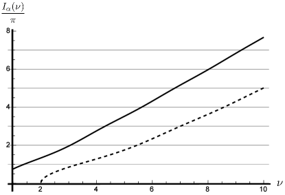
Figure 2: Plot of $\frac{I_{\alpha}(\nu)}{\pi}$ for $\alpha=1$ (continuous line ) $\alpha=2$ (broken line).

In Figure 2 we plot the graphs of $I_{\alpha}(\nu)/\pi$ for $\alpha=1,2$ as a function of $\nu$. These curves intersect the horizontal integer- lines (shown in the same figure) precisely at the locations of the energy eigenvalues, thus confirming remarkably the validity of Eq. (14). For comparison, we collect the graphical intersection points (computed using bisection search) in Table 1 where the exact eigenvalues obtained by Cavalcanti 9 are also listed.

Now, concerning potentials for which the wave functions are not obtainable in terms of known functions, a numerical routine can be outlined for the Dirac problem (following the prescription given in 11 for the non-relativistic ATM-quantization formula) yielding eigenvalue estimates, whose accuracy is only appreciable for larger eigenvalues–a feature that we do not understand completely at present. Therefore, a discussion of this scheme is not given here.

Table 1: First five values of $\nu=E^{2}/2g$ for select values of $\alpha=m/\sqrt{g}$. ($\hbar=c=1$).

	$\alpha=1$			$\alpha=2$
$\nu$	Exact	ATM		Exact	ATM
$\nu_{0}$	1.39627444057259	1.39627444809303		3.338595 40177509a	3.33859536647797
$\nu_{1}$	3.05676024015993	3.05676024192944		5.452160 76495126	5.45216075601056
$\nu_{2}$	4.30627664769999	4.30627665789798		7.006087 30469830	7.00608729608357
$\nu_{3}$	5.61521082352847	5.61521084997803		8.568945 86286508	8.56894588172436
$\nu_{4}$	6.80477121323347	6.80477123537566		9.978608 33615064	9.97860836439766

Next, we briefly mention another interesting application, to motivate further work. In fact, a detailed account of the same will be addressed in a follow- up paper. Particularly, we consider the problem of reconstructing the ground state wave function $\Psi_{o}$, for a given potential $V(x)$. The basic scheme is to assume the ground state energy $E_{o}$ to be a parameter and invert Eq. (14) to obtain $\Psi_{o}(E_{o})$. Although this is easier said than done, for simple power-law potentials $V(x)=g|x|^{n}(g>0,\ n\in\mathbb{N})$, using the ansatz

$$P=\exp\left(\int\frac{\mathrm{d}\xi}{\sum_{j=0}^{\infty}a_{j}\xi^{j}}\right)$$

in Eq. (10), one can obtain the coefficients $a_{j}$ by comparing powers of $\varepsilon_{o}$ on either side of the resulting equation. We would then resort to a variational principle to minimize the energy functional $E[\Psi]$, which is the expectation of the Dirac Hamiltonian w.r.t. the obtained parametric wave function, to find $E_{o}$. Similarly, recovery of the potential with knowledge of the ground state wave function is conceivable. However, this inversion problem is significantly complicated by the presence of the effective turning points, which depend on the potential implicitly.

V Conclusion

In this paper we analyzed the bound states of the one-dimensional Dirac equation for a scalar potential well $V(x)$ (satisfying two constraints laid in Section I), obtaining an exact energy quantization formula that extends the previously known analog for the Schrödinger equation. In fact, we could show that our formula reproduces this result in the appropriate non-relativistic limit. Further, we discussed the physically desirable symmetries of the quantization formula and applied the same to compute the energy eigenvalues for the potential $V=g|x|$.

Before concluding, we invite interested readers to strive for a completion of our relativistic quantization formula that would apply to an arbitrary scalar potential. Such a generalization must address two cases for which our analysis fails. First, the case of non-confining potentials: consider, for example, the one-dimensional Dirac equation with the scalar exponential potential $V(x)=Ae^{-\lambda x},\ \lambda>0$ 10 which, despite being repulsive everywhere, supports bound states for $A<0$. This is a consequence of the nature of coupling in the Dirac equation. Note that the exponential potential yields only one effective turning point, thus failing to satisfy ( at least) one of the constraints laid in Section I. As a result, our analysis would not apply to this case. Second, one must account for potentials that yield more than two effective turning points (a double well potential for instance). Unfortunately, the generalization of the analytic transfer matrix method to such potentials even for the non-relativistic problem stands open.

Acknowledgements

I would like to thank Dr. Hemalatha Thiagarajan, Dr. S.D. Mahanti and Dr. Mike Wilkes for critically reviewing the manuscript. Garv Chauhan and Avinash Prabhakar helped with the numerical results in Section IV. Thanks are also due to the anonymous reviewers for their valuable suggestions.

Appendix A

Let $\Psi$ be a bound state wave function, with its components $\psi_{1,2}$ satisfying Eqs. (1) and (2). Based on the properties of an admissible bound state wave function we deduce an useful property of the auxiliary function

$$P(\xi)=-\frac{\psi_{2}}{\psi_{1}}$$ (24)

which is well defined (and bounded) at any finite $\xi$ excepting the nodes of $\psi_{1}$. We show that

$$P(\xi_{L})<0<P(\xi_{R}),$$ (25)

where $\xi_{L}(\xi_{R})$ denotes the left(right) effective turning point (defined by $\vartheta(\xi_{L,R})+1=\varepsilon)$. Using this result we obtain the ‘ half phase losses’ at these turning points to be $\pi/2$ (Section II) . We recall that the chosen representation of the Dirac matrices allows us to work with a real $\Psi$ 4 . Hence, the inequality in proposition (25) is valid. In proving the above proposition, we require the following lemma.

Lemma 1.

The components of $\Psi$ cannot vanish simultaneously at any finite $\xi$. Equivalently, $\nexists~{}\xi\in\mathbb{R}|\Psi(\xi)=0$.

Proof.

Suppose there exists a $\xi_{o}$ such that $\Psi(\xi_{o})=0$. Consider a finite interval containing $\xi_{o}$ in which the wave function can be represented as ($A$, $B$ arbitrary coefficients)

$$\Psi(\xi)=\begin{pmatrix}1\\ \frac{~{}~{}~{}1}{1+\vartheta(\xi)+\varepsilon}\frac{\mathrm{d}}{\mathrm{d}\xi}\end{pmatrix}\left(A\psi_{1}^{(1)}(\xi)+B\psi_{1}^{(2)}(\xi)\right)$$ (26)

where $\psi_{1}^{(1)},\psi_{1}^{(2)}$ are the linearly independent solutions of the second order ODE

$$\ddot{\psi}_{1}-\left(\frac{\dot{\vartheta}(\xi)}{\varepsilon+\vartheta(\xi)+1}\right)\dot{\psi}_{1}+\left(\frac{\varepsilon+\vartheta(\xi)+1}{\varepsilon-\vartheta(\xi)-1}\right)\psi_{1}=0$$ (27)

that results from decoupling Eqs. (1) and (2).

Since $\Psi$ vanishes at $\xi_{o}$, the matrix equation

$$\begin{pmatrix}{\psi_{1}^{(1)}(\xi_{o})}&{\psi_{1}^{(2)}(\xi_{o})}\\ {\dot{\psi}_{1}^{(1)}(\xi_{o})}&{\dot{\psi}_{1}^{(2)}(\xi_{o})}\end{pmatrix}\begin{pmatrix}A\\ B\end{pmatrix}=0$$ (28)

must hold. Thus, in order to prevent the wave function from vanishing identically (i.e. $A=B=0$) on the interval, we must have $W(\psi_{1}^{(1)}(\xi_{o}),\psi_{1}^{(2)}(\xi_{o}))=0$ where $W$ is the Wronskian of the two functions. But this would contradict the linear independence of the solutions $\psi_{1}^{(1)},~{}\psi_{1}^{(2)}$ at $\xi_{o}$, hence such a $\xi_{o}$ does not exist. ∎

The regions where $\vartheta(\xi)+1<(>)\varepsilon$ are designated as allowed (forbidden) regions. Consider the properties

P1

$\psi_{1,2}\rightarrow 0$ as $|\xi|\rightarrow\infty$

P2

$\psi_{1,2}\neq 0$ for any $\xi$ (no nodes) in the forbidden region

which hold for any bound state wave function. We now prove inequality (25).

Proof.

Since Eqs. (1) and (2) remain form invariant under the transformation $\xi\mapsto-\xi(\Rightarrow\xi_{L}\mapsto\xi_{R})$ and $\psi_{1}\mapsto-\psi_{1}$ while $P\mapsto-P$, it suffices to prove any one of the two inequalities in (25). We focus on the right effective turning point $\xi_{R}$. The truth of proposition (25) rejects the possibility $\mathrm{sgn}[\psi_{1}(\xi_{R})]=\mathrm{sgn}[\psi_{2}(\xi_{R})]$ where $\mathrm{sgn}[~{}]$ is the signum function. To prove this we let $\psi_{1,2}(\xi_{R})>0$. From P2, it follows that $\psi_{1}>0$ for all $\xi>\xi_{R}$ (a forbidden region). Since $\psi_{2}(\xi_{R})>0$, Eq. (1) implies that $\dot{\psi}_{1}(\xi_{R})>0$. Since $\psi_{1}$ is increasing at $\xi_{R}$, it must attain at least one maximum before vanishing asymptotically as $\xi\rightarrow\infty$ (property P1), remaining positive-definite all along. Clearly, at the site of this maximum, $\dot{\psi}_{1}=0\Rightarrow\psi_{2}=0$, which contradicts property P2 for $\psi_{2}$. The other possibility $\psi_{1,2}(\xi_{R})<0$ (a ‘reflection’ of the previous case) is readily contradicted from form-invariance of Eqs. (1) and (2) under the transformation $\Psi\mapsto-\Psi$. Thus, $\mathrm{sgn}[\psi_{1}(\xi_{R})]=-\mathrm{sgn}[\psi_{2}(\xi_{R})]\Rightarrow P(\xi_{R})>0$. ∎

Finally, we show that

$$|P(\xi_{L,R})|<\infty$$ (29)

Proof.

Since $\psi_{1}$ and $\psi_{2}$ cannot vanish simultaneously (using the above Lemma), we need only show that an effective turning point cannot be a node of $\psi_{1}$. Consider $\xi_{R}$ as before. Assume $\psi_{1}(\xi_{R})=0$. From P1, $\psi_{1}\rightarrow 0$ as $\xi\rightarrow\infty$. Thus, $\psi_{1}$ must attain at least one minimum (maximum) if $\psi_{2}(\xi_{R})<0(>0)$ ($\because\mathrm{sgn}[\dot{\psi_{1}}]=\mathrm{sgn}[\psi_{2}]$), remaining negative (positive) definite all along. Similar to our earlier argument, at the site of this extremum $\psi_{2}=0$, which contradicts property P2 . Thus, $\psi_{1}(\xi_{R})\neq 0$. ∎

Appendix B

In this appendix we show that the integral (Eq. (10))

$$I=\int_{\xi_{L}}^{\xi_{R}}\frac{P\dot{\lambda}}{P^{2}+\lambda^{2}}\mathrm{d}\xi$$ (30)

exists for all potentials $\vartheta(\xi)$ that satisfy the constraints laid in Section I namely, (i) $\mathrm{min}\vartheta+1\geq 0$ and (ii) $1+\vartheta(\xi)=\varepsilon$ holds only at the two effective turning points $\xi_{L,R}$. In the analysis that follows, it is important to bear in mind that the components $\psi_{1,2}$ of a bound state wave function $\Psi$ have only finite number of zeros (or nodes) for $\xi_{L}<\xi<\xi_{R}$. Furthermore, between two consecutive nodes of $\psi_{1}$ there exists exactly one node of $\psi_{2}$ and vice-versa, which is a consequence of the fact that between two consecutive nodes of $\psi_{1}$ (say) there exists at least one extreme point of $\psi_{1}$ at which $\psi_{2}\propto\dot{\psi_{1}}=0$ (see Eq. (2)). Since this argument holds good for both $\psi_{1}$ and $\psi_{2}$, there could at the most be one node of $\psi_{2}$ between two consecutive nodes of $\psi_{1}$.

Now, we show that $I$ does not fail to exist due to the singularity at $\xi_{R}$. To do so, we focus on an interval $[\xi_{a},\xi_{R})$ where $\xi_{a}$ is greater than the largest among the nodes of $\psi_{1}$, $\psi_{2}$ and the (only) point of minimum of $\vartheta$ (denoted by $\xi_{c}$). Defining

$$I_{a}\mathrel{\hbox to0.0pt{\raisebox{1.29167pt}{$\cdot$}\hss}\raisebox{-1.29167pt}{$\cdot$}}=\int_{\xi_{a}}^{\xi_{R}}\frac{P\dot{\lambda}}{P^{2}+\lambda^{2}}\mathrm{d}\xi$$ (31)

we have

$$|I_{a}|\leq\int_{\xi_{a}}^{\xi_{R}}\left|\frac{P\dot{\lambda}}{P^{2}+\lambda^{2}}\right|\mathrm{d}\xi\leq\int_{\xi_{a}}^{\xi_{R}}\left|\frac{\dot{\lambda}}{P}\right|\mathrm{d}\xi$$ (32)

Using Eq. (11) we find

$$|\dot{\lambda}|=\frac{\varepsilon}{1+\vartheta+\varepsilon}\frac{|\dot{\vartheta}|}{\sqrt{\varepsilon^{2}-(1+\vartheta)^{2}}}$$

Also, as $1+\mathrm{min}\vartheta\geq 0$ (constraint (i)),

$$\frac{\varepsilon}{1+\vartheta+\varepsilon}\leq 1$$

combining these results, we obtain

$$|I_{a}|\leq\int_{\xi_{a}}^{\xi_{R}}\frac{|\dot{\vartheta}|}{\sqrt{\varepsilon^{2}-(1+\vartheta)^{2}}}\frac{\mathrm{d}\xi}{|P|}$$

$$=\int_{\xi_{a}}^{\xi_{R}}\frac{\dot{\vartheta}}{\sqrt{\varepsilon^{2}-(1+\vartheta)^{2}}}\frac{\mathrm{d}\xi}{|P|}$$ (33)

since $\dot{\vartheta}(\xi)>0$ for $\xi>\xi_{c}$. Integrating the r.h.s. of (33) by parts we obtain

$$|I_{a}| \leq\frac{\pi}{2|P(\xi_{R})|}-\frac{\sin^{-1}\left(\frac{1+\vartheta(\xi_{a})}{\varepsilon}\right)}{|P(\xi_{a})|}$$

$$-\int_{\xi_{a}}^{\xi_{R}}\sin^{-1}\left(\frac{1+\vartheta}{\varepsilon}\right)\frac{\mathrm{d}}{\mathrm{d}\xi}\left(\frac{1}{|P|}\right)\mathrm{d}\xi$$

Note that $|P(\xi_{a})|$ is non-zero and finite, owing to the choice of the point $\xi_{a}$ and so is $|P(\xi_{R})|$ (inequalities (25) and (29)). The r.h.s above can be bounded from above by its absolute value leading to

$$|I_{a}|\leq\frac{\pi}{2}\left(\frac{1}{|P(\xi_{R})|}+\frac{1}{|P(\xi_{a})|}+\int_{\xi_{a}}^{\xi_{R}}\left|\frac{\mathrm{d}}{\mathrm{d}\xi}\left(\frac{1}{|P|}\right)\right|\mathrm{d}\xi\right)$$ (34)

Note that, $\mathrm{sgn}(P(\xi))=\mathrm{sgn}(P(\xi_{R}))$ for all $\xi_{a}<\xi<\xi_{R}$, as $P$ doesn’t cross the $\xi$ axis (no nodes of $\psi_{2}$). Thus, $|P|=P$ (see inequality (25)). Furthermore, the derivative of $1/P$ has no zeros in this interval, since

$$\frac{\mathrm{d}}{\mathrm{d}\xi}\left(\frac{1}{P}\right)=0\Rightarrow P^{2}=\frac{1+\vartheta-\varepsilon}{1+\vartheta+\varepsilon}<0$$

which refutes the fact that $P$ is real in the chosen representation of the Dirac matrices. Therefore,

$$\int_{\xi_{a}}^{\xi_{R}}\left|\frac{\mathrm{d}}{\mathrm{d}\xi}\left(\frac{1}{|P|}\right)\right|\mathrm{d}\xi =\int_{\xi_{a}}^{\xi_{R}}\frac{\mathrm{d}}{\mathrm{d}\xi}\left(\frac{1}{P}\right)\mathrm{d}\xi$$

$$=\frac{1}{P(\xi_{R})}-\frac{1}{P(\xi_{a})}$$

Substituting this result in inequality (34) we obtain

$$|I_{a}|\leq\frac{\pi}{P(\xi_{R})}$$ (35)

which is finite (due to inequalities (25) and (29)). A similar argument works for the left turning point.

References

- (1) Cao, Zhuangqi, et al. “Quantization scheme for arbitrary one- dimensional potential wells.” Physical Review A 63.5 (2001): 054103.
- (2) Z. Cao, & C. Yin, Advances in One-Dimensional Wave Mechanics. Springer (2014).
- (3) H. Ying, Z. Fan-Ming, Y. Yan-Fang, & L. Chun-Fang, Energy eigenvalues from an analytical transfer matrix method. Chinese Physics B, 19(4), 040306 (2010).
- (4) Coutinho, F. A. B., Nogami, Y., & Toyama, F. M. (1988). General aspects of the bound state solutions of the one‐dimensional Dirac equation. American Journal of Physics, 56(10), 904-907.
- (5) Hiller, J. R. (2002). Solution of the one–dimensional Dirac equation with a linear scalar potential. American Journal of Physics, 70(5), 522-524.
- (6) Shirokov, D. S. (2014). Method of generalized contractions and Pauli’s theorem in Clifford algebras. arXiv preprint arXiv:1409.8163.
- (7) Strange, P. (1998). Relativistic Quantum Mechanics: with applications in condensed matter and atomic physics. Cambridge University Press.
- (8) Kennedy, P. (2002). The Woods–Saxon potential in the Dirac equation. Journal of Physics A: Mathematical and General, 35(3), 689.
- (9) Cavalcanti, R. M. (2002). Comment on “Fun and frustration with quarkonium in a 1+1 dimension,” by RS Bhalerao and B. Ram [Am. J. Phys. 69 (7 ), 817–818 (2001)]. American Journal of Physics, 70(4), 451-452.
- (10) de Castro, A. S., & Hott, M. (2005). Exact closed-form solutions of the Dirac equation with a scalar exponential potential. Physics Letters A, 342(1), 53-59.
- (11) A. Hutem, & C. Sricheewin, Ground-state energy eigenvalue calculation of the quantum mechanical well via analytical transfer matrix method. European Journal of Physics, 29(3), 577 (2008).
- (12) NIST Digital Library of Mathematical Functions. http:// dlmf.nist.gov/, Release 1.0.10 of 2015-08-07. Online companion to [OLBC10].
- (13) Lebedev, N. N., & Silverman, R. A. (1972). Special functions and their applications. Courier Corporation.
- (14) Vafek, O., & Vishwanath, A. (2013). Dirac fermions in solids- from high Tc cuprates and graphene to topological insulators and Weyl semimetals, Annual Review of Condensed Matter Physics, Vol: 5 Pages: 83-112, DOI: 10.1146/annurev-conmatphys-031113-133841 (2014)