Nonlinear modulation of the HI power spectrum on ultra-large scales. I

Abstract

Intensity mapping of the neutral hydrogen brightness temperature promises to provide a three-dimensional view of the universe on very large scales. Nonlinear effects are typically thought to alter only the small-scale power, but we show how they may bias the extraction of cosmological information contained in the power spectrum on ultra-large scales. For linear perturbations to remain valid on large scales, we need to renormalize perturbations at higher order. In the case of intensity mapping, the second-order contribution to clustering from weak lensing dominates the nonlinear contribution at high redshift. Renormalization modifies the mean brightness temperature and therefore the evolution bias. It also introduces a term that mimics white noise. These effects may influence forecasting analysis on ultra-large scales.

I Introduction

Mapping of the integrated 21cm emission from neutral hydrogen (HI) within unresolved sources will allow us to cover very large volumes of the observable universe with upcoming radio telescopes. This promises to deliver excellent precision in measuring the standard cosmological parameters Bull:2014rha , as well as new opportunities to probe signals on ultra-large scales, such as primordial non-Gaussianity and horizon-scale relativistic effects Hall:2012wd ; Camera:2013kpa ; Santos:2015gra ; Alonso:2015uua ; Raccanelli:2015vla ; Alonso:2015sfa ; Fonseca:2015laa ; Baker:2015bva .

The ability to extract precise cosmological information from an experiment is dependent on accurate understanding of the theoretical model. On scales $k\lesssim k_{\rm nl}=0.2h(1+z)^{2/(2+n_{s})}\,\text{Mpc}^{-1}$ (where $n_{s}=0.96$ is the primordial spectral index), gravitational evolution of large-scale structure can be analyzed via cosmological perturbations Smith:2002dz . For scales $k\ll k_{\rm nl}$, it is commonly assumed that one need not go beyond linear order. This is valid for cold dark matter (CDM) perturbations, which obey precise energy and momentum conservation, but not necessarily for tracers of the underlying CDM distribution.

It was shown in Heavens:1998es that mode coupling in the biased density field contributes power on large scales which becomes important on Hubble scales. This potential threat to the validity of linear perturbation theory on large scales can be mitigated by renormalization McDonald:2006mx ; McDonald:2009dh ; Chan:2012jx ; Nishizawa:2012db ; Assassi:2014fva . Renormalization leads to a change in the mean (zero-order) density and in the bias parameters for the tracer. In addition, it introduces a noise-like term McDonald:2006mx ; McDonald:2009dh ; Assassi:2014fva .

We employ this renormalization technique to study the HI brightness temperature after reionization. Up to second order in perturbation theory, the mean HI brightness temperature is modified by a term that depends on redshift and a coarse-graining scale. At $z\lesssim 1.5$, this term is proportional to a nonlinear bias parameter, while for $z\gtrsim 1.5$, it is dominated by a nonlinear weak lensing term. We point out that the renormalization of mean brightness temperature leads to a renormalization of the evolution bias parameter, which modifies the linear power spectrum on horizon scales. The main implication is that cosmological constraints on horizon scales need to incorporate nonlinear effects that flow from renormalization.

Our fiducial model is determined by the Planck 2015 best-fit values Ade:2015xua ; in particular, $h=H_{0}/100=0.673$, $\Omega_{m0}=1-\Omega_{\Lambda 0}=0.315$. A busy reader can skip section II which covers the perturbation theory (with details given in Appendix A). Section III covers the nonlinear (Gaussian) bias (with details for HI in Appendix B), and the basic ideas of renormalization are introduced and then implemented in redshift space. We discuss our results in section IV and conclude in section V.

II Fluctuations in HI brightness temperature

The brightness temperature observed (in redshift space) is given by Hall:2012wd

$$T^{\rm obs}(z,{{\bf{e}}}) = \frac{3\pi^{2}}{4}\frac{\hbar^{3}A_{10}}{k_{B}E_{21}}\,n(z,{\bf e})J(z,{\bf e})\,,$$ (1)

where $z$ is the redshift of the source, ${{\bf{e}}}$ is the unit direction of the source, $E_{21}$ is the proper energy of the emitted photons, and $A_{10}=2.869\times 10^{-15}{\rm s}^{-1}$ is the emission rate. The number density of HI atoms is $n$ and $J$ is the Jacobian of the map between real and redshift space [see (A)].

The observed temperature is expanded up to second order:

$$T^{\rm obs}(z,{{\bf{e}}}) = \bar{T}(z)\Big{[}1+\Delta_{T}^{\text{\tiny(1)}}(z,{{\bf{e}}})+\frac{1}{2}\Delta^{\text{\tiny(2)}}_{T}(z,{{\bf{e}}})\Big{]}\,,$$ (2)

where we use $\Delta_{T}$ to denote the quantity observed in redshift space. The mean brightness temperature is

$$\bar{T}(z) = \frac{3\pi^{2}}{4}\frac{\hbar^{3}A_{10}}{k_{B}E_{21}}\,\frac{\bar{n}(z)a(z)^{3}}{\mathcal{H}(z)}\approx 566h\frac{\Omega_{\text{\tiny{HI}}}(z)}{0.003}(1+z)^{2}\frac{H_{0}}{\mathcal{H}(z)}\,\,\mu{\rm K}.$$ (3)

Here $\Omega_{\text{\tiny{HI}}}$ is the comoving HI mass density in units of the current critical density.

The observed fractional temperature perturbation $\Delta_{T}$ is related to the fractional number overdensity $\delta_{n}$ in real space as follows (see Appendix A for details):

$$\Delta_{T}^{\text{\tiny(1)}}(z,{{\bf{e}}}) = \delta_{n}^{\text{\tiny(1)}}+\delta^{\text{\tiny(1)}}z-\delta^{\text{\tiny(1)}}k^{0}+\frac{1}{\mathcal{H}}\frac{\mbox{d}\delta^{\text{\tiny(1)}}z}{\mbox{d}\lambda}+\left(b_{e}-2\mathcal{H}-\frac{\mathcal{H}^{\prime}}{\mathcal{H}}\right)\delta^{\text{\tiny(1)}}\lambda\,,$$ (4)

$$\Delta^{\text{\tiny(2)}}_{T}(z,{{\bf{e}}}) = \delta^{\text{\tiny(2)}}_{n}+\delta^{\text{\tiny(2)}}z-\delta^{\text{\tiny(2)}}k^{0}-\omega_{{}_{{\text{\tiny$\|$}}}}^{\text{\tiny(2)}}+\frac{1}{\mathcal{H}}\frac{\mbox{d}\delta^{\text{\tiny(2)}}z}{\mbox{d}\lambda}+\left(b_{e}-2\mathcal{H}-\frac{\mathcal{H}^{\prime}}{\mathcal{H}}\right)\delta^{\text{\tiny(2)}}\lambda$$ (5)

$$+2\left[\delta^{\text{\tiny(1)}}k^{0}-\delta^{\text{\tiny(1)}}z-\frac{1}{\mathcal{H}}\frac{\mbox{d}\delta^{\text{\tiny(1)}}z}{\mbox{d}\lambda}\right]\left[\delta^{\text{\tiny(1)}}k^{0}-\delta_{n}^{\text{\tiny(1)}}\right]+2\left[\frac{1}{\mathcal{H}}\frac{\mbox{d}\delta^{\text{\tiny(1)}}z}{\mbox{d}\lambda}\right]^{2}$$

$$+2\delta^{\text{\tiny(1)}}\lambda\left[\left(\delta_{n}^{\text{\tiny(1)}}-\frac{1}{\mathcal{H}}\frac{\mbox{d}\delta^{\text{\tiny(1)}}z}{\mbox{d}\lambda}+\delta^{\text{\tiny(1)}}z-\delta^{\text{\tiny(1)}}k^{0}\right)\left(b_{e}-2\mathcal{H}-\frac{\mathcal{H}^{\prime}}{\mathcal{H}}\right)-\frac{\mathcal{H}^{\prime}}{\mathcal{H}^{2}}\frac{\mbox{d}\delta^{\text{\tiny(1)}}z}{\mbox{d}\lambda}\right]$$

$$+[\delta^{\text{\tiny(1)}}\lambda]^{2}\left[b_{e}^{2}+\frac{\mbox{d}b_{e}}{\mbox{d}\lambda}-4\mathcal{H}\left(b_{e}-\mathcal{H}\right)-2\frac{\mathcal{H}^{\prime}}{\mathcal{H}}\left(b_{e}-2\mathcal{H}-2\frac{\mathcal{H}^{\prime}}{\mathcal{H}}\right)-\frac{\mathcal{H}^{\prime\prime}}{\mathcal{H}}\right]$$

$$+2\left[\delta^{\text{\tiny(1)}}\lambda{\Delta_{T}^{\text{\tiny(1)}}}^{\prime}+\Delta x_{{}_{{\text{\tiny$\|$}}}}^{\text{\tiny(1)}}\partial_{{}_{{\text{\tiny$\|$}}}}\Delta_{T}^{\text{\tiny(1)}}+\Delta x_{\bot}^{\text{\tiny(1)}i}\nabla_{\bot i}\Delta_{T}^{\text{\tiny(1)}}\right]\,.$$

Here $k^{a}=\mbox{d}x^{a}/\mbox{d}\lambda$ is the photon 4-momentum, $\Delta x^{a}$ is the perturbed physical position, $\omega$ is the metric vector perturbation and $\|$ and $\bot$ denote projection along and transverse to ${\bf{e}}$. The evolution bias is defined by the mean number density:

$$b_{e}=-\mathcal{H}(z)\frac{\mbox{d}\ln[\bar{n}(1+z)^{-3}]}{\mbox{d}\ln(1+z)}.$$ (6)

From now on, for convenience we will often drop the superscript (1) for first-order perturbations.

• Background: We calculate $\Omega_{\text{\tiny{HI}}}$ from a simple halo model using

  $$\Omega_{\text{\tiny{HI}}}(z)=\frac{1}{(1+z)^{3}}\frac{\rho_{\text{\tiny{HI}}}(z)}{\rho_{c0}}\,,\quad\mbox{with}\quad\rho_{\text{\tiny{HI}}}(z)=\int_{M_{\text{min}}}^{M_{\text{max}}}\mbox{d}M\,n_{h}(M)M_{\text{\tiny{HI}}}(M)\,,$$ (7)

  where $\rho_{c0}=3H^{2}_{0}/(8\pi G)$ and $n_{h}$ is the halo mass function. See Appendix B for details.

• First-order perturbation: In Poisson gauge [see (49)], the full first-order perturbation is given by (A):

  $$\Delta_{T}^{\text{\tiny(1)}}(z,{{\bf{e}}}) = \delta_{n}^{\text{\tiny(1)}}-\frac{1}{\mathcal{H}}\partial^{2}_{{}_{{\text{\tiny$\|$}}}}v+\frac{1}{\mathcal{H}}\left(b_{e}-2\mathcal{H}-\frac{\mathcal{H}^{\prime}}{\mathcal{H}}\right)\partial_{{}_{{\text{\tiny$\|$}}}}v+\frac{1}{\mathcal{H}}\Psi^{\prime}-\frac{1}{\mathcal{H}}\left(b_{e}-3\mathcal{H}-\frac{\mathcal{H}^{\prime}}{\mathcal{H}}\right)\Phi$$

  $$+\frac{1}{\mathcal{H}}\left(b_{e}-2\mathcal{H}-\frac{\mathcal{H}^{\prime}}{\mathcal{H}}\right)\int_{\lambda_{o}}^{\lambda}\mbox{d}\tilde{\lambda}(\Phi^{\prime}+\Psi^{\prime})\,,$$

  where $v$ is the velocity potential. We have dropped the subscript $s$ for the source and set the observer-dependent monopole and dipole part to zero [see (A)]. Equation (• ‣ II) is in agreement with (17) of Hall:2012wd .

  The second term is the linear Kaiser redshift space distortion (RSD) term, followed by the Doppler term, the rate of change of the curvature potential, the gravitational redshift term and finally the integrated Sachs-Wolfe term. The third to the last terms are due to relativistic lightcone effects, and are suppressed on subhorizon scales Hall:2012wd . Note that there is no weak lensing contribution to the HI temperature at first order.

  A further horizon-scale term arises when we introduce the scale-independent bias. The relation $\delta_{n}=b\delta_{m}$, where $b=b(z)$, is only physical (and thus gauge-invariant) if expressed in the matter rest-frame, i.e. in comoving-synchronous gauge Hall:2012wd :

  $$\delta^{\text{\tiny(1)}}_{n}=b\delta^{{\rm cs}(1)}_{m}+(3\mathcal{H}-b_{e})v.$$ (9)

• Second-order perturbation: The second-order perturbations of the galaxy number counts that are observed on the lightcone in redshift space, were recently computed by Bertacca:2014dra ; Bertacca:2014wga ; Yoo:2014sfa ; DiDio:2014lka ; Bertacca:2014hwa . The extremely lengthy expressions are however not directly applicable to the case of intensity mapping which we are treating. In Appendix A we compute $\Delta^{\text{\tiny(2)}}_{T}(z,{{\bf{e}}})$, using the approach developed in Umeh:2012pn ; Umeh:2014ana . The full expression is unmanageable, and we make a consistent approximation that generalizes the Kaiser approximation Kaiser:1987qv to second order:

  $$\Delta^{\text{\tiny(2)}}_{T}(z,{{\bf{e}}}) = \delta_{n}^{\text{\tiny(2)}}-\frac{1}{\mathcal{H}}\partial^{2}_{{}_{{\text{\tiny$\|$}}}}v^{\text{\tiny(2)}}\overbrace{-\frac{2}{\mathcal{H}}\delta_{n}\partial^{2}_{{}_{{\text{\tiny$\|$}}}}v+2\left(\frac{1}{\mathcal{H}}\partial^{2}_{{}_{{\text{\tiny$\|$}}}}v\right)^{2}-\frac{2}{\mathcal{H}}\partial_{{}_{{\text{\tiny$\|$}}}}v\left[\partial_{{\text{\tiny$\|$}}}\delta_{n}-\frac{1}{\mathcal{H}}\partial_{{\text{\tiny$\|$}}}^{3}v\right]}^{\text{nonlinear RSD}}$$

  $$+\underbrace{2\left[\nabla_{\bot i}\delta_{n}-\frac{1}{\mathcal{H}}\nabla_{\bot i}\partial_{{\text{\tiny$\|$}}}^{2}v\right]\int_{0}^{\chi}\mbox{d}\tilde{\chi}(\tilde{\chi}-\chi)(\nabla^{i}_{\bot}\Phi+\nabla_{\bot}^{i}\Psi)}_{\text{nonlinear lensing}}+\underbrace{\frac{2}{\mathcal{H}}\partial_{{\text{\tiny$\|$}}}v\left[\delta^{\prime}_{n}-\frac{1}{\mathcal{H}_{s}}\partial_{{\text{\tiny$\|$}}}^{2}v^{\prime}\right]}_{\text{nonlinear time perturbation}}.$$

  The nonlinear RSD terms recover the result of Heavens:1998es ; Verde:1998zr for the galaxy number density. The nonlinear lensing term is $\Delta x_{\bot}^{\text{\tiny(1)}i}\nabla_{\bot i}\Delta_{T}^{\text{\tiny(1)}}$, i.e. the contraction of the weak lensing deflection angle with the transverse gradient of the first-order (density + RSD) term. This is the dominant nonlinear correction to Heavens:1998es ; Verde:1998zr . The time perturbation term is subdominant in the power spectrum – but it may be more important in the bispectrum. There are many further terms that we have neglected because they are strongly suppressed on sub-Hubble scales.

Relationship with galaxy number density

We derive a covariant mapping between the perturbation of observed brightness temperature and the perturbation of observed galaxy number density. If we count the observed number of HI atoms per solid angle and per redshift instead of galaxies, we find that the observed brightness temperature is given by Hall:2012wd

$$T^{\rm obs}(z,{\bf{e}}) = \frac{3\pi^{2}}{4}\frac{\hbar^{3}A_{10}}{k_{B}E_{21}^{2}}\frac{n^{\tiny{\text{obs}}}(z,{\bf{e}})}{D_{A}(z)^{2}}\,,$$ (11)

where $D_{A}$ is the angular diameter distance. Expanding in perturbations we find

$$\Delta_{T}^{\text{\tiny(1)}} = \Delta_{n}^{\text{\tiny(1)}}-2\frac{\delta D_{A}}{\bar{D}_{A}}\,,$$ (12)

$$\Delta^{(2)}_{T} = \Delta^{(2)}_{n}-2\frac{\delta^{\text{\tiny(2)}}D_{A}}{\bar{D}_{A}}-4\Delta_{n}\frac{\delta D_{A}}{\bar{D}_{A}}+6\left(\frac{\delta D_{A}}{\bar{D}_{A}}\right)^{2}-4\left[\delta\lambda\left(\frac{\delta D_{A}}{\bar{D}_{A}}\right)^{\prime}+\Delta x_{{}_{{\text{\tiny$\|$}}}}\partial_{{}_{{\text{\tiny$\|$}}}}\left(\frac{\delta D_{A}}{\bar{D}_{A}}\right)+\Delta x_{\bot}^{i}\nabla_{\bot i}\left(\frac{\delta D_{A}}{\bar{D}_{A}}\right)\right].$$ (13)

Here $\Delta_{n}$ is the fractional HI galaxy number overdensity observed in redshift space, before magnification bias is applied. At linear order, there is an accidental symmetry whereby $\Delta^{\text{\tiny(1)}}_{T}$ is obtained from the magnification bias corrected $\Delta_{n}$, by simply setting the slope of the luminosity function to $s=2/5$ Hall:2012wd . Equation (12) is in exact agreement with (23) of Hall:2012wd and (13) is its second-order extension.

III Nonlinear perturbations and renormalization

In order to illustrate the main idea, we start by ignoring the corrections due to observation in redshift space and by focusing on sub-Hubble scales, where the difference between comoving-synchronous and Newtonian gauges in (9) may be ignored. Fluctuations in number density should average to zero over large enough volumes, i.e.

$$\delta_{n}(z,{\bf{x}})=\frac{n(z,{\bf{x}})-\langle{n}\rangle(z)}{\langle{n}\rangle(z)}\quad\Rightarrow\quad\langle\delta_{n}(z,{\bf{x}})\rangle=0.$$ (14)

Within standard cosmological perturbation theory, we normally assume that $\langle{n}\rangle(z)=\bar{n}(z)=\bar{n}^{\text{FLRW}}(z)$, i.e we assume that $\bar{n}$ is determined by the background FLRW spacetime. However this does not take account of the complexities of relating a tracer to the underlying CDM distribution.

A bias model is needed to relate $\delta_{n}$ to the CDM overdensity $\delta_{m}$. We assume that the primordial perturbations are Gaussian, and use an Eulerian local bias model, applied up to second order:

$$\delta_{n}(z,{\bf{x}})=b_{1}(z)\delta_{m}(z,{\bf{x}})+\frac{1}{2}b_{2}(z)\big{[}\delta_{m}(z,{\bf{x}})\big{]}^{2}\,.$$ (15)

As a consequence, the average in (15) no longer vanishes:

$$\langle\delta_{n}\rangle(z)=b_{2}(z)\sigma^{2}_{S}(z),\quad\sigma^{2}_{S}(z)=\int_{k_{\text{min}}}^{k_{S}}{\mbox{d}^{3}k\over(2\pi)^{3}}P_{m}(z,k).$$ (16)

Here $\sigma^{2}_{S}$ is the variance of $\delta_{m}$ and $k_{S}$ is the small-scale cutoff.

A mathematically consistent way of ensuring zero average is via renormalization McDonald:2006mx ; McDonald:2009dh ; Assassi:2014fva ; Nishizawa:2012db . This involves subtracting $b_{2}\sigma^{2}_{S}/2$ from both sides of (15). The right-hand side will then have zero average, by (16), while the left-hand side will define a renormalized fluctuation $\delta^{R}_{n}=\delta_{n}-b_{2}\sigma^{2}_{S}/2$.

Renormalization of $\delta_{n}$ must leave invariant the physical number density $n$. This is achieved by renormalization of the background number density, $\bar{n}$, which in turn induces a renormalization of the bias parameters:

$$\bar{n}^{R}=\bar{n}\big{(}1+b_{2}\sigma^{2}_{S}/2\big{)},~{}~{}~{}b_{a}^{R}={b_{a}\over\big{(}1+b_{2}\sigma^{2}_{S}/2\big{)}}.$$ (17)

Putting this together, we have

$$\delta_{n}^{{R}}\equiv\frac{n-\bar{n}^{R}}{\bar{n}^{R}}=b_{1}^{R}\delta_{m}+\frac{1}{2}{b_{2}^{R}}\left[(\delta_{m})^{2}-\sigma^{2}_{S}\right]\quad\Rightarrow\quad\langle\delta_{n}^{{R}}\rangle=0.$$ (18)

Note that the fundamental physical quantity (i.e $n$) is independent of the cutoff scale chosen to regulate the integral in $\sigma^{2}_{S}$, i.e., $\partial n/\partial k_{S}=0$ Assassi:2014fva .

An important consequence of renormalization was not mentioned in McDonald:2009dh ; Assassi:2014fva ; Nishizawa:2012db , since these papers did not include the horizon-scale general relativistic terms that we have in (• ‣ II). This consequence is that the evolution bias $b_{e}$, which appears in the coefficients of most of the general relativistic terms, will be renormalized as a result of renormalization of the mean number density. Using equations (6) and (17), $b_{e}$ is modified by $n$-renormalization as

$$b_{e}^{R}=b_{e}-\mathcal{H}(z)\frac{\mbox{d}\ln(1+b_{2}\sigma^{2}_{S}/2)}{\mbox{d}\ln(1+z)}\,.$$ (19)

As a result, the linear power spectrum of the observed fractional temperature fluctuations will be modified on horizon scales by renormalization.

The power spectrum may be computed by expanding (18) in Fourier space (we suppress the $z$-dependence):

$$\delta_{n}^{R}({\bf{k}})=b_{1}^{R}\delta_{m}({\bf{k}})+\frac{1}{2}\bigg{[}\int\frac{\mbox{d}^{3}k_{1}}{(2\pi)^{3}}\frac{\mbox{d}^{3}k_{2}}{(2\pi)^{3}}\delta_{m}({\bf{k}}_{1})\delta_{m}({\bf{k}}_{2})(2\pi)^{3}\delta^{D}\!({\bf{k}}-{\bf{k}}_{1}-{\bf{k}}_{2})\left[b_{2}^{R}+b_{1}^{R}F_{2}({\bf{k}}_{1},{\bf{k}}_{2})\right]-b_{2}^{R}\sigma^{2}_{S}\,\delta^{D}\!({\bf{k}})\bigg{]},$$ (20)

where $P_{m}$ is the linear matter power spectrum and $F_{2}$ is the standard nonlinear density kernel, which we approximate using a matter-dominated model:

$$F_{2}({\bf{k}}_{1},{\bf{k}}_{2})=\frac{5}{7}+\frac{1}{2}\left({k_{1}\over k_{2}}+{k_{2}\over k_{1}}\right){{\bf{k}}_{1}\cdot{\bf{k}}_{2}\over k_{1}k_{2}}+\frac{2}{7}\left({{\bf{k}}_{1}\cdot{\bf{k}}_{2}\over k_{1}k_{2}}\right)^{2}.$$ (21)

Computing $\langle\delta_{n}^{R}({\bf{k}})\delta_{n}^{R}({\bf{k}}^{\prime})\rangle$, we find that the contributions of the $\sigma_{S}^{2}$ term exactly cancel out and the power spectrum of the renormalized fractional number overdensity is

$${P}_{\delta^{R}_{n}}(k)=\left(b_{1}^{R}\right)^{2}P_{m}(k)+\frac{1}{2}\int\frac{\mbox{d}^{3}k_{1}}{(2\pi)^{3}}\Big{[}b_{2}^{R}+b_{1}^{R}F_{2}({\bf{k}}_{1},{\bf{k}}-{\bf{k}}_{1})\Big{]}^{2}P_{m}(|{\bf{k}-{\bf{k}}_{1}|})P_{m}({k}_{1}).$$ (22)

The $b_{2}^{R}$ term leads to constant power on very large scales Heavens:1998es ; McDonald:2009dh ; BeltranJimenez:2010bb :

$$k\to 0~{}\Rightarrow~{}{P}_{\delta^{R}_{n}}(k)\to\frac{1}{2}\left(b_{2}^{R}\right)^{2}\int\frac{\mbox{d}^{3}k_{1}}{(2\pi)^{3}}P_{m}^{2}({k}_{1}),$$ (23)

where we used $F_{2}({\bf{k}},-{\bf{k}})=0$. It is possible to renormalize the power spectrum by subtracting this constant power from both sides of (22). In this approach, the constant-power contribution is treated as part of the noise budget Heavens:1998es ; McDonald:2006mx ; McDonald:2009dh :

$${P}^{R}_{\delta^{R}_{n}}(k) = \left(b_{1}^{R}\right)^{2}P_{m}(k)+\frac{1}{2}\int\frac{\mbox{d}^{3}k_{1}}{(2\pi)^{3}}\left\{\big{[}b_{2}^{R}+b_{1}^{R}F_{2}({\bf{k}}_{1},|{\bf{k}-{\bf{k}}_{1}|})\big{]}^{2}P_{m}(|{\bf{k}-{\bf{k}}_{1}|})-\left(b_{2}^{R}\right)^{2}P_{m}(k_{1})\right\}P_{m}({k}_{1}),$$ (24)

$${P}_{\delta^{R}_{n}}(k) = {P}^{R}_{\delta^{R}_{n}}(k)+N_{\rm eff},~{}~{}N_{\rm eff}=\frac{1}{2}\left(b_{2}^{R}\right)^{2}\int\frac{\mbox{d}^{3}k_{1}}{(2\pi)^{3}}P_{m}^{2}({k}_{1}).$$ (25)

Here we follow a different approach, consistent with Jeong:2008rj ; BeltranJimenez:2010bb . We see the constant-power term as containing cosmological information rather than noise, i.e. we treat it as a nonlinear correction to the power spectrum. In this view, we use the unrenormalized power spectrum (22). The two approaches differ only in the interpretation of the correction to the linear power spectrum on ultra-large scales.

Renormalization in redshift space for the brightness temperature

We now extend the established renormalization procedure from real space to the observed redshift space, in the case of the observed fractional HI brightness temperature perturbation:

$$\Delta_{T}(z,{\bf{e}})=\frac{T^{\text{obs}}(z,{\bf{e}})-\langle T^{\text{obs}}\rangle(z)}{\langle T^{\text{obs}}\rangle(z)}.$$ (26)

The sky average of $\langle\Delta_{T}\rangle$ is zero by definition, but if we assume that $\langle T^{\text{obs}}\rangle=\bar{T}^{\text{FLRW}}$, we get a nonzero value. In order to ensure that $\langle\Delta_{T}\rangle=0$, we have to renormalize the background temperature.

In observed redshift space, the average is more complicated because of the nonlinear lensing contribution in (• ‣ II). After performing the sky integral, we find that

$$\langle\Delta_{T}\rangle(z)=\frac{1}{2}\langle\Delta_{T}^{\text{\tiny(2)}}\rangle(z)=\left\{b_{2}(z)+4\Big{[}b_{1}(z)+\frac{1}{5}f(z)\Big{]}T_{\kappa}(z)\right\}\sigma^{2}_{S}(z)\,,$$ (27)

where $f=\mbox{d}\ln D/\mbox{d}\ln a$ is the growth rate and $D$ the growing mode of the linear matter overdensity, and

$$T_{\kappa}(z)=\frac{\Omega_{m0}H_{0}^{2}}{D(z)}\int_{0}^{\chi}\mbox{d}\tilde{\chi}\,[1+z(\tilde{\chi})]D(\tilde{\chi})(\tilde{\chi}-\chi){\tilde{\chi}\over\chi},$$ (28)

is a transfer function for the weak lensing convergence. The sky average of the nonlinear lensing term is the only redshift-space contribution to the monopole.

We renormalize the background temperature and its fluctuations by adding and subtracting $\langle\Delta_{T}\rangle$ to (26):

$$\bar{T}^{R} = \bar{T}\big{(}1+\langle\Delta_{T}\rangle\big{)},$$ (29)

$$\Delta_{T}^{R}({\bf{k}},\mu) = {\Delta_{T}^{R}}^{\text{\tiny(1)}}({\bf{k}},\mu)+\frac{1}{2}\left[{\Delta_{T}^{R}}^{\text{\tiny(2)}}({\bf{k}},\mu)-\langle\Delta_{T}\rangle\delta^{D}({\bf{k}})\right],\quad\mu={{\bf{k}}\cdot{{\bf{e}}}\over k},~{}~{}\langle\Delta_{T}^{R}({\bf{k}},\mu)\rangle=0,$$ (30)

where we suppressed the $z$-dependence. Here the renormalized first- and second-order parts are

$${\Delta_{T}^{R}}^{\text{\tiny(1)}}({\bf{k}},\mu) = {\delta_{m}({\bf{k}})\over 1+\langle\Delta_{T}\rangle}\left[b_{1}+f\mu^{2}+\mathcal{A}\,\frac{\mathcal{H}^{2}}{k^{2}}+i\mu\mathcal{B}\,\frac{\mathcal{H}}{k}\right]\,,$$ (31)

$${\Delta_{T}^{R}}^{\text{\tiny(2)}}({\bf{k}},\mu) = {1\over 1+\langle\Delta_{T}\rangle}\int\frac{\mbox{d}^{3}k_{1}}{(2\pi)^{3}}\frac{\mbox{d}^{3}k_{2}}{(2\pi)^{3}}\delta_{m}({\bf{k}}_{1})\delta_{m}({\bf{k}}_{2})(2\pi)^{3}\delta^{D}\!({\bf{k}}-{\bf{k}}_{1}-{\bf{k}}_{2})\bigg{[}b_{2}+b_{1}F_{2}({\bf{k}}_{1},{\bf{k}}_{2})$$ (32)

$$+f\mu^{2}G_{2}({\bf{k}}_{1},{\bf{k}}_{2})+\mathcal{K}_{\text{R}}({\bf{k}}_{1},{\bf{k}}_{2})+\mathcal{K}_{\text{L}}({\bf{k}}_{1},{\bf{k}}_{2})+i\mathcal{K}_{\text{T}}({\bf{k}}_{1},{\bf{k}}_{2})\bigg{]}.$$

In order to define the HI bias physically at linear order, we used the definition (9) and we applied (15) in comoving-synchronous gauge. For convenience we have omitted the cs superscript – i.e., $\delta_{m}$ in the above and following equations is understood to be $\delta^{\rm cs}_{m}$. Note that we do not need to extend the comoving-synchronous definition to second order, because the difference contains only terms that we are neglecting at second order.

The $\mathcal{A}$ and $\mathcal{B}$ terms in (31) are the coefficients of the first-order potential and Doppler terms in (• ‣ II):

$$\mathcal{A} = f\left(3-\frac{b_{e}^{R}}{\mathcal{H}}-\frac{3}{2}\Omega_{m}\right)-\left[2-\frac{b_{e}^{R}}{\mathcal{H}}+\frac{\mathcal{H}^{\prime}}{\mathcal{H}^{2}}\right]\left[\frac{3}{2}\Omega_{m}+3\int_{0}^{z}\mbox{d}\tilde{z}\,\Omega_{m}(\tilde{z})\frac{\mathcal{H}^{2}(\tilde{z})D(\tilde{z})}{\mathcal{H}^{2}(z)D(z)}[f(\tilde{z})-1]\right],$$ (33)

$$\mathcal{B} = -f\left(2-\frac{b_{e}^{R}}{\mathcal{H}}+\frac{\mathcal{H}^{\prime}}{\mathcal{H}^{2}}\right)\,.$$ (34)

The renormalized background temperature is equivalent to a renormalized background number density by (3), so that the evolution bias is renormalized:

$$b_{e}^{R}=b_{e}-\mathcal{H}(z)\frac{\mbox{d}\ln\big{(}1+\langle\Delta_{T}\rangle_{L}\big{)}}{\mbox{d}\ln(1+z)}\,.$$ (35)

We have introduced a smoothing scale $L$ (in units of ${h}^{-1}\,$Mpc). For a top-hat window function on a scale $L$, (27) becomes:

$$\langle\Delta_{T}\rangle_{L}=\int\frac{\mbox{d}^{3}k}{(2\pi)^{3}}P_{m}(k)\left[\big{|}W({kL})\big{|}^{2}b_{2}+4W({kL})\left(b_{1}+\frac{1}{5}f\right)T_{\kappa}\right]\,,\quad W({kL})=3\left[\frac{\sin(kL)}{(kL)^{3}}-\frac{\cos(kL)}{(kL)^{2}}\right].$$ (36)

We show the fractional difference, $\Delta b^{R}_{e}/b_{e}=(b_{e}^{R}-b_{e})/b_{e}$, in Fig. 1, for various values of $L$. For $L=10{h}^{-1}\,$Mpc, the difference is $\sim 1\%$ and for $L\gg 10{h}^{-1}\,$Mpc, we recover the FLRW limit as expected. The difference grows as $L$ is decreased below $10{h}^{-1}\,$Mpc. For $L\lesssim 2{h}^{-1}\,$Mpc, we need to go beyond second-order perturbation theory. The crossover point at $z\sim 1.5$ arises due to competititon between the nonlinear HI bias and the nonlinear lensing effect. The nonlinear bias in (35) is negative and the lensing contribution ${T}_{\kappa}$ is positive, and they cancel at $z\sim 1.5$. The fractional difference is dominated by the nonlinear bias for $z\lesssim 1.5$ and for $z\gtrsim 1.5$ by the nonlinear lensing effect.

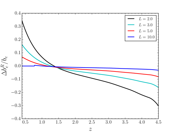
Figure 1: Fractional difference in the evolution bias due to nonlinear effects for different values of the smoothing scale $L$ (in units of $h^{-1}\,$Mpc).

The kernels in (32) are as follows. $G_{2}({\bf{k}}_{1},{\bf{k}}_{2})$ is the kernel for peculiar velocity at second order, which we approximate by its form in a matter-dominated universe:

$$G_{2}({\bf{k}}_{1},{\bf{k}}_{2})=\frac{3}{7}+\frac{1}{2}\left({k_{1}\over k_{2}}+{k_{2}\over k_{1}}\right){{\bf{k}}_{1}\cdot{\bf{k}}_{2}\over k_{1}k_{2}}+\frac{4}{7}\left({{\bf{k}}_{1}\cdot{\bf{k}}_{2}\over k_{1}k_{2}}\right)^{2}.$$ (37)

The ${\cal K}$ kernels encode the nonlinear effects from mode coupling: ${\cal K}_{\rm R}$ – RSD (velocity-velocity and velocity-density); ${\cal K}_{\rm L}$ – lensing (lensing-density and lensing-Kaiser); ${\cal K}_{\rm T}$ – time perturbation (velocity-density and velocity- velocity). These are given by:

$$\mathcal{K}_{\text{R}}({\bf{k}}_{1},{\bf{k}}_{2}) = {b_{1}f}\left[\mu_{1}^{2}+\mu_{2}^{2}+\mu_{1}\mu_{2}\left({k_{1}\over k_{2}}+{k_{2}\over k_{1}}\right)\right]+f^{2}\left[2\mu_{1}^{2}\mu_{2}^{2}+{\mu_{1}\mu_{2}}\left(\mu_{1}^{2}\frac{k_{1}}{k_{2}}+\mu_{2}^{2}\frac{k_{2}}{k_{1}}\right)\right]\,,$$ (38)

$$\mathcal{K}_{\text{L}}({\bf{k}}_{1},{\bf{k}}_{2}) = 3\sqrt{1-\mu^{2}_{1}}\sqrt{1-\mu_{2}^{2}}\bigg{[}\left({k_{1}\over k_{2}}+{k_{2}\over k_{1}}\right)b_{1}+f\left(\frac{k_{1}\mu^{2}_{1}}{k_{2}}+\frac{k_{2}\mu^{2}_{2}}{k_{1}}\right)\bigg{]}T_{\kappa}\,,$$ (39)

$$\mathcal{K}_{\text{T}}({\bf{k}}_{1},{\bf{k}}_{2}) = -(1+z)f\mathcal{H}\left[b_{1}f+\frac{\mbox{d}b_{1}}{\mbox{d}z}+\left(\mu^{2}_{1}+\mu_{2}^{2}\right)\left(f+\frac{\mbox{d}}{\mbox{d}z}\ln(f\mathcal{H})\right)\right]\left(\frac{\mu_{1}}{k_{1}}+\frac{\mu_{2}}{k_{2}}\right),$$ (40)

where

$$\mu_{a}={{\bf{k}}_{a}\cdot{{\bf{e}}}\over k_{a}},\quad a=1,2,\dots$$ (41)

The power spectrum of observed HI temperature fluctuations in a distant observer approximation then follows from (31) and (32):

$${P}_{T}({k},\mu) = \big{(}\bar{T}\big{)}^{2}\left[b_{1}+f\mu^{2}+\mathcal{A}\,\frac{\mathcal{H}^{2}}{k^{2}}+i\mu\mathcal{B}\,\frac{\mathcal{H}}{k}\right]\left[b_{1}+f\mu^{2}+\mathcal{A}\,\frac{\mathcal{H}^{2}}{k^{2}}-i\mu\mathcal{B}\,\frac{\mathcal{H}}{k}\right]P_{m}(k)$$ (42)

$$+\frac{\big{(}\bar{T}\big{)}^{2}}{2}\int\frac{\mbox{d}^{3}k_{1}}{(2\pi)^{3}}\bigg{[}b_{2}+b_{1}F_{2}({\bf{k}}_{1},{\bf{k}}-{\bf{k}}_{1})+f\mu^{2}G_{2}({\bf{k}}_{1},{\bf{k}}-{\bf{k}}_{1})$$

$$+\mathcal{K}_{\text{R}}({\bf{k}}_{1},{\bf{k}}-{\bf{k}}_{1})+\mathcal{K}_{\text{L}}({\bf{k}}_{1},{\bf{k}}-{\bf{k}}_{1})+i\mathcal{K}_{\text{T}}({\bf{k}}_{1},{\bf{k}}-{\bf{k}}_{1})\bigg{]}^{2}P_{m}(|{\bf{k}}-{\bf{k}}_{1}|)P_{m}({k}_{1}).$$

Once again, this power spectrum has a nonzero constant-power limit as $k\to 0$:

$${P}_{T}\to\frac{\bar{T}^{2}}{2}\int\frac{\mbox{d}^{3}k_{1}}{(2\pi)^{3}}\Big{[}b_{2}+3(1-\mu^{2}_{1})\left(b_{1}+\mu^{2}_{1}f\right)T_{\kappa}\Big{]}^{2}P^{2}_{m}({k}_{1}).$$ (43)

The monopole of the power spectrum is

$$P^{\ell=0}_{T}(k) = (\bar{T})^{2}\bigg{[}b_{1}^{2}+\frac{2}{3}b_{1}f+\frac{1}{5}f^{2}+\frac{1}{3}\left[\mathcal{B}^{2}+2\left(3b_{1}+f\right)\mathcal{A}\right]\frac{\mathcal{H}^{2}}{k^{2}}+\mathcal{A}^{2}\frac{\mathcal{H}^{4}}{k^{4}}\bigg{]}P_{m}(k)+\frac{1}{2}\int_{-1}^{1}\mbox{d}\mu\,P^{(2)}_{T}(k,\mu),$$ (44)

where $P^{(2)}_{T}$ is the second order part of (42).

IV Results and Discussion

There are two key nonlinear effects on the ultra-large scale power spectrum that we have identified – modification of the evolution bias and constant power that mimics white noise on horizon scales. These could potentially affect the standard analysis on horizon scales which assumes that linear theory is valid.

Here we compute the nonlinear modifications to the power spectrum $P_{T}$ of the renormalized HI temperature fluctuations, as given in (42) and (44). For this computation, we compute the HI bias parameters using a standard prescription in Appendix B. We set the limits of the convolution integral in (42) following Carlson:2009it : $(k_{1}^{\rm min},k_{1}^{\rm max})=(10^{-4},10^{4})h^{-1}\,$Mpc.

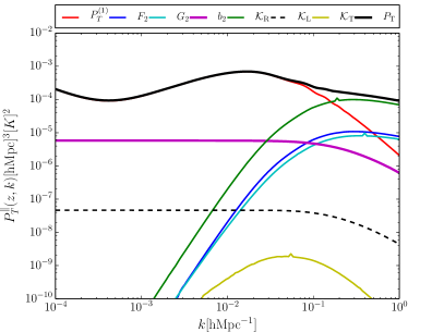
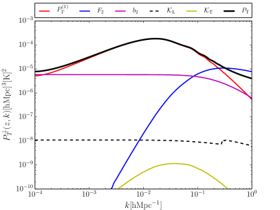
Figure 2: Power spectrum $P_{T}$ of the renormalized observed HI brightness temperature, at $z=0.5$. Left: along the line of sight; Right: transverse to the line of sight. The solid black curve shows the total power and the red curve is the linear part $P_{T}^{(1)}$ of (42). The remaining curves show the nonlinear effects from: $F_{2}$ – second-order density perturbations, $G_{2}$ – RSD from second-order velocity, $b_{2}$ – HI bias, $\mathcal{K}_{\rm R}$ – RSD from mode coupling, $\mathcal{K}_{\rm L}$ – lensing effect from mode coupling, $\mathcal{K}_{\rm T}$ – time perturbation from mode coupling.

In practice, the choice of the smoothing scale $1/k_{S}$ will be connected to the resolution of the experiment. This scale cannot however be smaller than the scale $1/k_{\rm nl}$ if we wish to remain in the regime of validity of the perturbative approach. In our calculations we set $k_{S}\sim k_{\rm nl}\sim L^{-1}$. We note that although the results can be sensitive to the exact value of $k_{\rm nl}$, this is not an issue as long as $1/k_{S}>1/k_{\rm nl}$. The calculations will then only depend on $k_{S}$ but this is just a statement that the power spectrum needs to be smoothed on the resolution scale of the experiment in order to compare to observations.

We do not use a window function to regulate the convolution integral in (42). Careful analysis using a smoothed density field and angular power spectrum will be presented elsewhere.

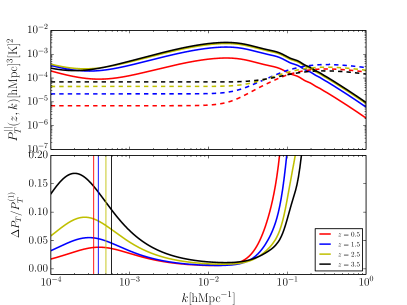
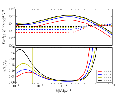
Figure 3: Power spectrum $P_{T}$ of the renormalized observed HI brightness temperature at various redshifts. Left panels: along the line of sight; right panels: monopole. Upper panels: Solid lines are the linear power spectrum, dashed lines the nonlinear power. Lower panels: The fractional difference due to nonlinear effects. Vertical lines indicate the comoving Hubble scale.

Figure 2 illustrates the amount of power contributed by the terms in (42), for $\mu=1,0$. The term responsible for non-vanishing of the average of $\Delta_{T}$ contributes constant power on large scales. At linear order, the horizon-scale GR effects in $P_{T}^{(1)}$ become important near the horizon ($k\sim\mathcal{H}$) and dominate on super-Hubble scales ($k<\mathcal{H}$). (We have not computed the horizon-scale GR effects at second order, since this in itself is a major task which is left for further work.) Along the line of sight ($\mu=1$), the nonlinear RSD from mode coupling (via $\mathcal{K}_{\text{R}}$) clearly dominates the nonlinear contribution $P_{T}^{(2)}$ at $k\gtrsim 0.05$. For $k\gtrsim 0.1$, it dominates over even the linear power spectrum $P_{T}^{\text{\tiny(1)}}$. At BAO scales, its contribution is $\sim 10\%$. As expected $\mathcal{K}_{\text{R}}$ vanishes for $\mu=0$.

We quantify in Fig. 3 the total second-order effect on the linear power spectrum, focusing on large scales. The fractional difference is defined as $\Delta P_{T}/P_{T}^{\text{\tiny(1)}}=\big{[}P_{T}-P_{T}^{\text{\tiny(1)}}\big{]}/P_{T}^{\text{\tiny(1)}}$. The contribution of the dominant constant power term peaks around the horizon scale $k=\mathcal{H}(z)$. The constant power from the lensing term $\mathcal{K}_{\text{L}}$ dominates over the constant power from nonlinear bias at about $z\sim 1$ .

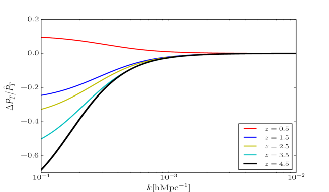
Figure 4: Effect of renormalized evolution bias on the monopole of the power spectrum on large scales. (The line of sight power spectrum is identical.) The smoothing scale for the evolution bias is set at $L=5(1+z)^{-{2}/{(2+n_{s})}}h^{-1}\,$Mpc.

We also quantify the error on the power spectrum associated with using the bare evolution bias (6), instead of the renormalized evolution bias (35). To this end, we define the fractional difference as $\Delta P_{T}/\tilde{P}_{T}\equiv\big{(}{{P_{T}}-\tilde{P}_{T}}\big{)}/{\tilde{P}_{T}}$, where $\tilde{P}_{T}$ is the power spectrum with bare evolution bias, given by (6). Figure 4) shows that the difference could be more than 20% on horizon scales.

Furthermore, what about third-order terms that we have neglected? These terms can contribute to the one-loop correction to the tree-level power spectrum through cross-correlation with first-order terms. Here we argue that the effect of third-order terms will be sub-dominant on the large scales that we are interested in. The brightness temperature up to third order is

$$T^{\rm obs}(z,{{\bf{e}}}) = \bar{T}(z)\Big{[}1+\Delta_{T}^{\text{\tiny(1)}}(z,{{\bf{e}}})+\frac{1}{2}\Delta^{\text{\tiny(2)}}_{T}(z,{{\bf{e}}})+\frac{1}{3!}\Delta_{T}^{\text{\tiny(3)}}(z,{{\bf{e}}})\Big{]}.$$ (45)

Assuming Gaussian initial conditions, the main contribution to the mean brightness temperature after renormalization will come from the third-order bias term. For a local Eulerian bias model, $\delta_{n}=b_{1}\delta_{m}+b_{2}\delta^{2}_{m}/2+b_{3}\delta^{3}_{m}/3!$, the ensemble average of the third-order term is given by Bernardeau:2001qr :

$$b_{3}\big{\langle}\delta_{m}^{3}\big{\rangle}=3b_{3}\big{\langle}\big{(}\delta_{m}^{\text{\tiny(1)}}\big{)}^{2}\delta_{m}^{\text{\tiny(2)}}\big{\rangle}=\frac{34}{7}b_{3}\big{(}\sigma^{2}_{S}\big{)}^{2}.$$ (46)

Using a Sheth-Torman mass function Sheth:1999mn ; Sheth:2001dp , we can show that $-1<b_{3}<1$ for $z\leq 3.5$, as seen in Fig. 5 (see appendix B). This implies that for $\sigma^{2}_{S}<1$, we have $(\sigma^{2}_{S})^{2}<\sigma^{2}_{S}$. Therefore $\langle\Delta^{\text{\tiny(3)}}_{T}\rangle<\langle\Delta^{\text{\tiny(2)}}_{T}\rangle$, i.e the contribution from third-order fluctuations to the mean brightness temperature is sub-dominant.

The mode coupling term $\langle\Delta_{T}^{\text{\tiny(1)}}(z,{\bf{k}})\Delta_{T}^{\text{\tiny(3)}}(z,{\bf{k}})\rangle$, will contribute to the power spectrum at one-loop as follows:

$$P^{(13)}_{T}(k,\mu) = \frac{1}{3}\left(b_{1}+f\mu^{2}+\mathcal{A}\,\frac{\mathcal{H}^{2}}{k^{2}}+i\mu\mathcal{B}\,\frac{\mathcal{H}}{k}\right)P_{m}(k)\int\frac{\mathrm{d}^{3}k_{1}}{(2\pi)^{3}}P_{m}(k_{1})\mathcal{K}^{\text{\tiny(3)}}(k,{\bf{k}}_{1},-{\bf{k}}_{1},\mu),$$ (47)

where $\mathcal{K}^{\text{\tiny(3)}}$ is the kernel for all third-order terms. Although (47) is a one-loop contribution to the tree-level power spectrum, it does not appear as a convolution of two power spectra, i.e. it does not produce a coupling of power on small scales to ultra-large scales that can modify our results on those large scales. Also if we set $k_{1}=kr$, and take the limit $k\rightarrow 0$, the pre-factor in (47) goes to zero faster than the rate at which the $r$-integral goes to larger values.

Finally, it is important to point out that the expression for HI brightness temperature given in equation (1) is a special limit of the HI brightness temperature during the Epoch of Reionization (EoR):

$$\delta T=\bar{T}\bar{x}_{\text{\tiny{HI}}}\left(1+\delta_{n}\right)\left(1+\frac{\delta{x_{\text{\tiny{HI}}}}}{\bar{x}_{\text{\tiny{HI}}}}\right)\left(1+\frac{\delta{J}}{\bar{J}}\right)\left(1-\frac{T_{\text{\tiny{CMB}}}}{T_{s}}\right)$$ (48)

where $\bar{x}_{\text{\tiny{HI}}}$ is neutral fraction of hydrogen, $\delta x_{\text{\tiny{HI}}}$ is the perturbation in neutral fraction of hydrogen, $T_{\text{\tiny{CMB}}}$ is the temperature of the CMB, $\delta J$ is the perturbed Jacobian and $T_{s}$ is the spin temperature. Equation (48) reduces to equation (1) in the limit $T_{\text{\tiny{CMB}}}\ll T_{s}$. Despite these differences, the modulation of the HI power spectrum on ultra-large scales by nonlinear effects we discussed at low-z will also be applicable during the EoR because the dominant nonlinear terms come from the perturbed Jacobian ($\delta J$) and not from $T_{s}$ and $T_{\text{\tiny{CMB}}}$ which we neglected.

V Conclusion

We derived for the first time the second-order perturbation of the HI brightness temperature in the post-reionization universe, focusing on the dominant nonlinear redshift space distortion terms and the nonlinear lensing term. We find that:

• The physical mean density of HI or the mean brightness temperature is modified by nonlinear terms that depend on redshift and the cutoff scale. By smoothing over structures on scales where perturbation theory may not be trusted, we showed that this could lead to more than 20% change to the power spectrum on large scales.

• The constant power on large scales associated with nonlinear evolution of biased tracers can significantly affect the power spectrum on horizon scales. The boost in amplitude could affect the signal to noise ratio for possible detection of general relativistic effects and primordial non-Gaussianity from intensity mapping.

However, the power spectrum is not observable. In order to determine whether these effects do lead to observable consequences, we need to compute the observed angular power spectrum $C_{\ell}(z,z^{\prime})$. This is a subject for further investigation.

Appendix A Brightness temperature in perturbation theory

Here we provide details for the perturbation calculation up to second order, using the approach developed in Umeh:2012pn ; Umeh:2014ana . We consider a perturbed FLRW spacetime in the Poisson gauge assuming a flat background metric

$$\mbox{d}\hat{s}^{2} = a^{2}\mbox{d}s^{2}=a^{2}\left[-(1+2\Phi+\Phi^{\text{\tiny(2)}})\mbox{d}\eta^{2}+2\omega_{i}\mbox{d}x^{i}\mbox{d}\eta+\left((1-2\Psi-\Psi^{\text{\tiny(2)}})\delta_{ij}+h_{ij}\right)\mbox{d}x^{i}\mbox{d}x^{j}\right]\,.$$ (49)

Here the proper time is related to conformal time by $\mbox{d}t=a\mbox{d}\eta$. $\Phi$ is the first-order Newtonian gravitational potential, $\Psi$ is scalar curvature perturbation, and $\omega_{i}=\omega_{i}^{\text{\tiny(V)}}$ and $h_{ij}=h_{ij}^{\text{\tiny(T)}}$ are the second-order vector and tensor contributions, their divergences vanish. Since the null structure is unchanged under conformal transformation, the metric $\hat{g}_{ab}$ associated with the line element $\mbox{d}\hat{s}^{2}$, i.e physical spacetime maps the null geodesic of the physical spacetime $\hat{g}_{ab}$ to a null geodesic on a perturbed Minkowski space time $g_{ab}$ with the affine parameter associated with each metric, transforming as $\mbox{d}\hat{\lambda}\rightarrow\mbox{d}\lambda=a^{-2}\mbox{d}{\lambda}$. The photon 4-vector transforms as $\hat{k}^{b}=a^{-2}k^{b}\Leftrightarrow\hat{k}_{a}=k_{a}$. For the matter 4-velocity, we have $\hat{u}^{a}=a^{-1}u^{a}\Leftrightarrow\hat{u}_{a}=au_{a}$ . Hence, the photon energy transforms as $\hat{E}=-\hat{u}_{b}\hat{k}^{b}=-a\,u_{b}k^{b}=aE$. For any tensor $S$ we expand it up to second order as

$$\hat{S}=\bar{S}+\delta^{\text{\tiny(1)}}S+\frac{1}{2}\delta^{\text{\tiny(2)}}S\,.$$ (50)

We expand the 4-velocity, $u^{a}$, of a matter field using (49) up to second order

$$u^{0} = 1-\Phi+\frac{3}{2}\Phi^{2}-\frac{1}{2}\Phi^{\text{\tiny(2)}}+\frac{1}{2}\bar{\partial}_{i}v\bar{\partial}^{i}v$$ (51)

$$u^{i} = \bar{\partial}^{i}v+\frac{1}{2}v^{i}{}^{\text{\tiny(2)}}+\frac{1}{2}\bar{\partial}^{i}v^{\text{\tiny(2)}}$$ (52)

The perturbed photon tangent vector is calculated from the geodesic $k^{a}\nabla_{a}k^{b}=0$ and the redshift is given by

$$1+\hat{z}=1+\delta z+\frac{1}{2}\delta^{\text{\tiny(2)}}z = \frac{k^{a}u_{a}|_{s}}{k^{b}u_{b}|_{o}}$$ (53)

The background conformal time or the conformal metric affine parameter is mapped to the conformal time in redshift space according to

$$\lambda=\nu+\delta\lambda+\frac{1}{2}\delta^{\text{\tiny(2)}}\lambda$$ (54)

Hence the physical scale factor is related to the background scale factor through Taylor series expansion

$$a(\lambda) = a(\nu_{s})\left[1+\mathcal{H}_{s}\delta\lambda+\frac{1}{2}\left(\mathcal{H}_{s}\,{\delta}^{\text{\tiny(2)}}\lambda+\left(\mathcal{H}^{\prime}_{s}+\mathcal{H}_{s}^{2}\right)(\delta\lambda)^{2}\right)\right]\,,$$ (55)

where we have performed the Taylor series expansion around the position of the physical position of the source. For consistency, we could define a homogeneous redshift in terms of the physical scale factor as

$$(1+z_{s}) = \frac{a(\nu_{o})}{a(\nu_{s})}\,.$$ (56)

We have also made the following replacements in (55)

$$\frac{1}{a}\frac{\mbox{d}a}{\mbox{d}\lambda}\bigg{|}_{\nu_{s}}=\mathcal{H}_{s},\qquad\frac{1}{a}\frac{\text{d}^{2}a}{\text{d}\lambda^{2}}\bigg{|}_{\nu_{s}}=\left(\mathcal{H}^{\prime}_{s}+\mathcal{H}^{2}_{s}\right)\,.\,,$$ (57)

Inverting (53) and using (55) leads to

$$\frac{1}{(1+z_{s})} = \frac{a(\nu_{s})}{a(\nu_{o})}\left[1+\left(\mathcal{H}_{s}\delta\lambda-\delta z\right)+\frac{1}{2}\left(\mathcal{H}_{s}\delta^{\text{\tiny(2)}}\lambda-\delta^{\text{\tiny(2)}}z+2(\delta z)^{2}-2\mathcal{H}_{s}\delta z\delta\lambda+\left(\mathcal{H}^{\prime}_{s}+\mathcal{H}^{2}_{s}\right)(\delta\lambda)^{2}\right)\right]\,.$$ (58)

Thus from (58), the background scale factor may now be re-defined in terms of the physical redshift using (56) and requiring that terms vanish at every order leads to

$$\delta\lambda = \frac{\delta z}{\mathcal{H}_{s}}\,,$$ (59)

$$\delta^{\text{\tiny(2)}}\lambda = \frac{1}{\mathcal{H}_{s}}\left[\delta^{\text{\tiny(2)}}z-(\delta z)^{2}\left(1+\frac{\mathcal{H}^{\prime}_{s}}{\mathcal{H}^{2}_{s}}\right)\right]\,.$$ (60)

For further details on this see Umeh:2014ana . In order to expand the Jacobian in (11), we need to relate the conformal time to the affine parameter associated with the physical metric according to ($\mbox{d}\eta\rightarrow\mbox{d}\lambda$)

$$\frac{\mbox{d}\lambda}{\mbox{d}{\hat{\lambda}}} = \frac{1}{a^{2}(\eta)}\left[1+\delta k^{0}+\frac{1}{2}\left(\omega_{{}_{{\text{\tiny$\|$}}}}+\delta^{\text{\tiny(2)}}k^{0}\right)\right]$$ (61)

and using (53) we link it to the physical redshift

$$\frac{\mbox{d}\lambda}{\mbox{d}{\hat{\lambda}}} = (1+\hat{z}_{s})^{2}\left[1+\left(\delta k^{0}-2\delta z\right)+\frac{1}{2}\left(\omega_{{}_{{\text{\tiny$\|$}}}}+\delta^{\text{\tiny(2)}}k^{0}-2\delta^{\text{\tiny(2)}}z+2\delta z\left(3\delta z-2\delta k^{0}\right)\right)\right]$$ (62)

Differentiating (53) wrt $\lambda$ gives

$$\frac{\mbox{d}\hat{z}}{\mbox{d}\lambda} = -\frac{\mathcal{H}(\eta)}{a(\eta)}\left[1+\delta z+\frac{1}{2}\delta^{\text{\tiny(2)}}z-\frac{1}{\mathcal{H}(\eta)}\left(\frac{\mbox{d}\delta z}{\mbox{d}\lambda}+\frac{1}{2}\frac{\mbox{d}\delta^{\text{\tiny(2)}}z}{\mbox{d}\lambda}\right)\right]$$ (63)

It is convenient now to re-express background $\mathcal{H}(\eta)$ and $a(\eta)$ in terms of the observed redshift

$$\frac{\mbox{d}\hat{z}}{\mbox{d}\lambda} = -\frac{\mathcal{H}(\nu)}{a(\nu)}\bigg{\{}1+\left[\delta z-\frac{1}{\mathcal{H}_{s}}\frac{\mbox{d}\delta z}{\mbox{d}\lambda}-\left(\mathcal{H}_{s}-\frac{\mathcal{H}^{\prime}_{s}}{\mathcal{H}_{s}}\right)\delta\lambda\right]+\frac{1}{2}\left[\delta^{\text{\tiny(2)}}z-\frac{1}{\mathcal{H}_{s}}\frac{\mbox{d}\delta^{\text{\tiny(2)}}z}{\mbox{d}\lambda}-\left(\mathcal{H}_{s}-\frac{\mathcal{H}^{\prime}_{s}}{\mathcal{H}_{s}}\right)\delta^{\text{\tiny(2)}}\lambda\right.$$

$$\left.+2\delta\lambda\left(\frac{\mbox{d}\delta z}{\mbox{d}\lambda}-\delta z\left(\mathcal{H}_{s}-\frac{\mathcal{H}^{\prime}_{s}}{\mathcal{H}_{s}}\right)\right)+(\delta\lambda)^{2}\left(\mathcal{H}_{s}^{2}-3\mathcal{H}^{\prime}_{s}+\frac{\mathcal{H}^{\prime\prime}_{s}}{\mathcal{H}_{s}}\right)\right]\bigg{\}}$$

Using (62), we substitute for $\mbox{d}\lambda$ and after some simplification we find

$$\frac{\mbox{d}\hat{z}}{\mbox{d}{\hat{\lambda}}} = -\frac{\mathcal{H}(\nu)}{a(\nu)^{3}}\bigg{\{}1+\left(\delta k^{0}-\delta z-\frac{1}{\mathcal{H}_{s}}\frac{\mbox{d}\delta z}{\mbox{d}\lambda}-\left(\mathcal{H}_{s}-\frac{\mathcal{H}^{\prime}_{s}}{\mathcal{H}_{s}}\right)\delta\lambda\right)+\frac{1}{2}\left[\delta^{\text{\tiny(2)}}k^{0}+\omega_{{}_{{\text{\tiny$\|$}}}}-\delta^{\text{\tiny(2)}}z-\frac{1}{\mathcal{H}_{s}}\frac{\mbox{d}\delta^{\text{\tiny(2)}}z}{\mbox{d}\lambda}\right.$$

$$\left.-\left(\mathcal{H}_{s}-\frac{\mathcal{H}^{\prime}_{s}}{\mathcal{H}_{s}}\right)\delta^{\text{\tiny(2)}}\lambda+2\left((\delta z)^{2}-\frac{2}{\mathcal{H}_{s}}\delta k^{0}\frac{\mbox{d}\delta z}{\mbox{d}\lambda}\right)+2\delta z\left(\frac{2}{\mathcal{H}_{s}}\frac{\mbox{d}\delta z}{\mbox{d}\lambda}-\delta k^{0}\right)+2\bigg{(}\frac{\mbox{d}\delta z}{\mbox{d}\lambda}+\delta z\left(\mathcal{H}_{s}-\frac{\mathcal{H}^{\prime}_{s}}{\mathcal{H}_{s}}\right)\right.$$

$$\left.-2\delta k^{0}\left(\mathcal{H}_{s}-\frac{\mathcal{H}^{\prime}_{s}}{\mathcal{H}_{s}}\right)\bigg{)}\delta\lambda+(\delta\lambda)^{2}\left(\mathcal{H}_{s}^{2}-3\mathcal{H}^{\prime}_{s}+\frac{\mathcal{H}^{\prime\prime}_{s}}{\mathcal{H}_{s}}\right)\right]\bigg{\}}$$

The Jacobian in (11) is then obtained by simply inverting (A)

$$J\equiv\bigg{|}\frac{\mbox{d}{\hat{\lambda}}}{\mbox{d}\hat{z}}\bigg{|} = \frac{a(\nu)^{3}}{\mathcal{H}(\nu)}\bigg{\{}1+\left(\delta z-\delta k^{0}+\frac{1}{\mathcal{H}_{s}}\frac{\mbox{d}\delta z}{\mbox{d}\lambda}+\left(\mathcal{H}_{s}-\frac{\mathcal{H}^{\prime}_{s}}{\mathcal{H}_{s}}\right)\delta\lambda\right)+\frac{1}{2}\left[\delta^{\text{\tiny(2)}}z-\delta^{\text{\tiny(2)}}k^{0}-\omega_{{}_{{\text{\tiny$\|$}}}}+\frac{1}{\mathcal{H}_{s}}\frac{\mbox{d}\delta^{\text{\tiny(2)}}z}{\mbox{d}\lambda}\right.$$

$$\left.+\left(\mathcal{H}_{s}-\frac{\mathcal{H}^{\prime}_{s}}{\mathcal{H}_{s}}\right)\delta^{\text{\tiny(2)}}\lambda+\delta\lambda\left[2\frac{\mbox{d}\delta z}{\mbox{d}\lambda}\left(1-2\frac{\mathcal{H}^{\prime}_{s}}{\mathcal{H}^{2}_{s}}\right)+2\delta z\left(\mathcal{H}_{s}-\frac{\mathcal{H}^{\prime}_{s}}{\mathcal{H}_{s}}\right)-2\delta k^{0}\left(\mathcal{H}_{s}-\frac{\mathcal{H}^{\prime}_{s}}{\mathcal{H}_{s}}\right)\right]+\right.$$

$$\left.(\delta\lambda)^{2}\left(\mathcal{H}^{2}_{s}-\mathcal{H}^{\prime}_{s}+2\left(\frac{\mathcal{H}^{\prime}_{s}}{\mathcal{H}_{s}}\right)-\frac{\mathcal{H}^{\prime\prime}_{s}}{\mathcal{H}_{s}}\right)-2\delta k^{0}\left(\delta z+\frac{1}{\mathcal{H}_{s}}\frac{\mbox{d}\delta z}{\mbox{d}\lambda}\right)+2\left((\delta k^{0})^{2}+\left(\frac{1}{\mathcal{H}_{s}}\frac{\mbox{d}\delta z}{\mbox{d}\lambda}\right)^{2}\right)\right]\bigg{\}}$$

For the HI number density we follow the standard prescription given in (50)to perturb it up to second order

$$n(\eta,x^{i})=\bar{n}(\eta)\left[1+\delta_{n}(\eta,x^{i})+\frac{1}{2}\delta^{\text{\tiny(2)}}_{n}(\eta,x^{i})\right]\,,$$ (67)

The background number density is then mapped to its equivalent in redshift space

$$\bar{n}({\eta}) = \bar{n}(\nu_{s})\left[1+\frac{\bar{n}^{\prime}}{\bar{n}}\delta\lambda+\frac{1}{2}\left(\frac{\bar{n}^{\prime}}{\bar{n}}\,{\delta}^{\text{\tiny(2)}}\lambda+\frac{\bar{n}^{\prime\prime}}{\bar{n}}(\delta\lambda)^{2}\right)\right]\,.$$ (68)

The rate of change of background number density along the line of sight define parameters that quantify our insufficient knowledge of the background spacetime, i.e the evolution bias parameters:

$$b_{e} = \frac{\mbox{d}\ln(a^{3}\bar{n}(\bar{\eta}))}{\mbox{d}\eta}=3\frac{a^{\prime}}{a}+\frac{\bar{n}^{\prime}}{\bar{n}}\,,$$ (69)

$$\frac{\mbox{d}b_{e}}{\mbox{d}\lambda} = -\left(b_{e}-3\mathcal{H}\right)\left(3\mathcal{H}-b_{e}\right)+3\mathcal{H}^{\prime}+\frac{\bar{n}^{\prime\prime}}{\bar{n}}\,.$$ (70)

Putting (A) and (67) into (11), we arrive at equations (4) and (5).

Using the photon geodesic $k^{a}\nabla_{a}k^{b}=0$, we calculate the weak lensing terms from the perturbed photon 4-vector, which at first order is given by

$$\delta k^{0}(\lambda_{s}) = -2(\Phi_{s}-\Phi_{o})+\int_{\lambda_{s}}^{\lambda_{o}}(\Phi^{\prime}+\Psi^{\prime})\mbox{d}\lambda$$ (71)

$$\delta k_{\|}(\lambda_{s}) = -(\Phi_{s}-\Phi_{o})+(\Psi_{s}-\Psi_{o})-\int_{\lambda_{s}}^{\lambda_{o}}(\Phi^{\prime}+\Psi^{\prime})\mbox{d}\lambda$$ (72)

$$\delta k^{i}_{\bot}(\lambda_{s}) = -\int_{\lambda_{s}}^{\lambda_{o}}\nabla^{i}_{\bot}(\Phi+\Psi)\mbox{d}\lambda\,,$$ (73)

where we have set the perturbation of the geodesic at the observer to zero, $\delta k^{a}(\lambda_{o})=0$. The radial component is obtained by projecting on $e^{i}$, while the transverse component comes from projecting with the screen space metric, $N_{ij}=\bar{g}_{ij}+u_{i}u_{j}-e_{i}e_{j}$. The perturbed position of the photon at first order is obtained by solving the following equation

$$\frac{\mbox{d}\delta x^{b}}{\mbox{d}\lambda}=\delta k^{b}-\delta k^{c}\partial_{c}x^{b}\,.$$ (74)

Using equations (71)–(73) in (74) we find

$$\delta\lambda = \frac{\delta z}{\mathcal{H}_{s}}=\frac{1}{\mathcal{H}_{s}}\left[(\partial_{{}_{{\text{\tiny$\|$}}}}v_{s}-\partial_{{}_{{\text{\tiny$\|$}}}}v_{o})-(\Phi_{s}-\Phi_{o})+\int_{\lambda_{o}}^{\lambda_{s}}(\Phi^{\prime}+\Psi^{\prime})\mbox{d}\lambda\right]\,,$$ (75)

$$\Delta x_{\|} = -\left(\Psi_{o}+\Phi_{o}\right)\left(\lambda_{o}-\lambda_{s}\right)+\int^{\lambda_{s}}_{\lambda_{o}}\left(\Phi+\Psi\right)\mbox{d}\lambda-\frac{1}{\mathcal{H}_{s}}\left[(\partial_{{}_{{\text{\tiny$\|$}}}}v_{s}-\partial_{{}_{{\text{\tiny$\|$}}}}v_{o})-(\Phi_{s}-\Phi_{o})+\int_{\lambda_{o}}^{\lambda_{s}}(\Phi^{\prime}+\Psi^{\prime})\mbox{d}\lambda\right],$$ (76)

$$\Delta x_{\bot}^{i} = -\int_{\lambda_{o}}^{\lambda_{s}}(\lambda_{s}-\lambda)(\nabla^{i}_{\bot}\Phi+\nabla_{\bot}^{i}\Psi)\mbox{d}\lambda=\int_{0}^{\chi_{s}}(\chi-\chi_{s})(\nabla^{i}_{\bot}\Phi+\nabla_{\bot}^{i}\Psi)\mbox{d}\chi\,.$$ (77)

Then the first order brightness temperature fluctuation (4) is given by

$$\Delta_{T}^{\text{\tiny(1)}}(z,{{\bf{e}}}) = \delta_{n}-\frac{1}{\mathcal{H}_{s}}\partial^{2}_{{}_{{\text{\tiny$\|$}}}}v_{s}+\frac{1}{\mathcal{H}_{s}}\left(b_{e}-2\mathcal{H}_{s}-\frac{\mathcal{H}^{\prime}_{s}}{\mathcal{H}_{s}}\right)\partial_{{}_{{\text{\tiny$\|$}}}}v_{s}+\frac{1}{\mathcal{H}_{s}}\Psi^{\prime}_{s}-\frac{1}{\mathcal{H}_{s}}\left(b_{e}-3\mathcal{H}_{s}-\frac{\mathcal{H}^{\prime}_{s}}{\mathcal{H}_{s}}\right)\Phi_{s}$$

$$+\frac{1}{\mathcal{H}_{s}}\left(b_{e}-2\mathcal{H}_{s}-\frac{\mathcal{H}^{\prime}_{s}}{\mathcal{H}_{s}}\right)\int_{\lambda_{o}}^{\lambda_{s}}(\Phi^{\prime}+\Psi^{\prime})\mbox{d}\lambda+\Delta_{T}^{\text{\tiny(1)}}(z,{\bf{x}}_{o})$$

where $\Delta_{T}^{\text{\tiny(1)}}(z,{\bf{x}}_{o})$ is a collection of all the terms measured at observer

$$\Delta_{T}^{\text{\tiny(1)}}(z,{\bf{x}}_{o}) = -\frac{1}{\mathcal{H}_{s}}\left(b_{e}-\mathcal{H}_{s}-\frac{\mathcal{H}^{\prime}_{s}}{\mathcal{H}_{s}}\right)\partial_{{}_{{\text{\tiny$\|$}}}}v_{o}+\frac{1}{\mathcal{H}_{s}}\left(b_{e}-3\mathcal{H}_{s}-\frac{\mathcal{H}^{\prime}_{s}}{\mathcal{H}_{s}}\right)\Phi_{o}$$ (79)

Recently, the second-order large-scale perturbations to the observed galaxy number counts have been computed by Bertacca:2014dra ; Bertacca:2014wga ; Yoo:2014sfa ; DiDio:2014lka ; Bertacca:2014hwa . These results do not cover the case of HI intensity mapping. Substituting for all the terms in the second-order fluctuation (5) leads to an unmanageably long expression. We take a consistent extension of the Kaiser approximation Kaiser:1987qv from first to second order, so as to reduce the complexity of the calculation. The full calculation will be presented elsewhere. Obtaining a consistent Kaiser limit up to second order requires that we set

$$\delta k^{0}\longrightarrow 0\,,\quad\delta k_{{\text{\tiny$\|$}}}\longrightarrow 0\,,\quad\delta^{\text{\tiny(2)}}k^{0}\longrightarrow 0\,,\quad\delta^{\text{\tiny(2)}}k_{{\text{\tiny$\|$}}}\longrightarrow 0\,,\quad\delta z\longrightarrow 0\,,\quad\delta^{\text{\tiny(2)}}z\longrightarrow 0\,.$$ (80)

These terms contain a Doppler term and gravitational potential terms, and products of these two terms. We do not set these terms to zero in the post-Born correction terms because post-Born correction terms already contain higher number of derivatives than other terms in the equation. Implementing the approximation of (80) in equations (4) and (5), we find

$$\Delta_{T}^{\text{\tiny(1)}}(z,{\bf{e}}) \approx \delta_{n}+\frac{1}{\mathcal{H}_{s}}\frac{\mbox{d}\delta z}{\mbox{d}\lambda}\,,$$ (81)

$$\Delta_{T}^{\text{\tiny(2)}}(z,{\bf{e}}) \approx \delta_{n}^{\text{\tiny(2)}}+\frac{1}{\mathcal{H}}\frac{\mbox{d}\delta^{\text{\tiny(2)}}z}{\mbox{d}\lambda}+2\left(\frac{1}{\mathcal{H}}\frac{\mbox{d}\delta z}{\mbox{d}\lambda}\right)^{2}+2\delta_{n}\left(\frac{1}{\mathcal{H}}\frac{\mbox{d}\delta z}{\mbox{d}\lambda}\right)+2\bigg{[}\frac{\delta z}{\mathcal{H}_{s}}{\Delta_{T_{b}}^{\text{\tiny(1)}}}^{\prime}+\Delta x_{{}_{{\text{\tiny$\|$}}}}\partial_{{}_{{\text{\tiny$\|$}}}}\Delta_{T_{b}}^{\text{\tiny(1)}}+\Delta x_{\bot}^{i}\nabla_{\bot i}\Delta_{T_{b}}^{\text{\tiny(1)}}\bigg{]}\,.$$ (82)

The last set of terms in (82) clearly show how the effect of weak lensing appears in an HI intensity map. Its appearance is solely due to the post-Born correction that must be included if one goes beyond linear order Hagstotz:2014qea . The derivative of the redshift with respect to $\lambda$ contains the redshift space distortion terms and they are given by

$$\frac{\mbox{d}\delta z}{\mbox{d}\lambda}=\partial{{}_{{\text{\tiny$\|$}}}}v^{\prime}-\partial_{{\text{\tiny$\|$}}}^{2}v+\partial{{}_{{\text{\tiny$\|$}}}}\Phi+\Phi^{\prime}\approx-\partial^{2}_{{}_{{\text{\tiny$\|$}}}}v\,,\qquad\frac{\mbox{d}\delta^{\text{\tiny(2)}}z}{\mbox{d}\lambda}\approx-\partial^{2}_{{}_{{\text{\tiny$\|$}}}}v^{\text{\tiny(2)}},$$ (83)

where we have implemented the derivatives of the conditions listed in (80).

Considering only the dominant terms in each case and putting these terms together, we obtain finally the key result of (• ‣ II).

Appendix B HI bias from halo bias

We calculate the bias parameters from a simple Sheth-Torman mass function Sheth:1999mn ; Sheth:2001dp :

$$b_{1} = 1+\left\langle\frac{(q\nu-1)}{\delta_{c}}+\frac{2p}{\delta_{c}\left(1+(q\nu)^{p}\right)}\right\rangle_{\tiny{\text{M}}}\,,$$ (84)

$$b_{2} = \frac{8}{21}\left(b_{1}-1\right)+\left\langle\frac{4\left(p^{2}+\nu pq\right)-(q\nu-1)\left(1+(q\nu)^{p}\right)-2p}{\delta^{2}_{c}\left(1+(q\nu)^{p}\right)}+\frac{1}{\delta_{c}^{2}}\left((q\nu)^{2}-2q\nu-1\right)\right\rangle_{\tiny{\text{M}}}\,$$ (85)

$$b_{3} = -\frac{236}{189}\left(b_{1}-1\right)-\frac{13}{7}\left(b_{2}-\frac{8}{21}\left(b_{1}-1\right)\right)+\bigg{<}-\frac{\left(3+3\nu q+3\nu^{2}q^{2}-\nu^{3}q^{3}\right)}{\delta_{c}^{3}}$$

$$+\frac{\left(8p^{3}+12p^{2}\left(1+\nu q\right)+p\left(6\nu^{2}q^{2}-2\right)\right)}{\delta_{c}^{3}\left(1+1+(\nu q)^{p}\right)}+6\frac{\left(1+2\nu q-\nu^{2}q^{2}\right)}{\delta_{c}^{3}}-24\frac{\left(p^{2}+\nu pq\right)}{\delta_{c}^{3}\left(1+(\nu q)^{p}\right)}$$

$$-4\frac{(1-\nu q)}{\delta_{c}^{3}}+8\frac{p}{\delta_{c}^{3}\left(1+(q\nu)^{p}\right)}\bigg{>}_{\rm M}\,,$$

where $q=0.707$ and $p=0.3$ are obtained from a fit to numerical simulations. The peak height is related to the variance $\sigma(M)$ of the density field smoothed on mass scale $M$ by $\nu=\left({\delta_{\text{c}}}/{\sigma_{\text{G}}}\right)^{2}.$ The averaging notation is defined by

$$X(z,{\bf{x}})=\left\langle X_{h}(z,{\bf{x}})\right\rangle_{\tiny{\text{M}}}=\frac{\int_{M_{-}}^{M_{+}}\mbox{d}M\left[X_{h}(z,{\bf{x}},M)M_{\text{\tiny{HI}}}(M)n_{h}(z,{\bf{x}},M)\right]}{\int_{M_{-}}^{M_{+}}\mbox{d}M\left[M_{\text{\tiny{HI}}}(M)n_{h}(z,{\bf{x}},M)\right],}$$ (87)

where $M_{-}$ and $M_{+}$ are the lower and upper limits of masses, which are related to the limits of circular velocity of galaxies that could house HI. These are obtained from the circular velocity constraint

$$v_{\text{circ}}=30\sqrt{1+z}\left(\frac{M}{10^{10}M_{\odot}}\right)^{1/3}~{}{\rm km\,s}^{-1}\,,$$ (88)

where we assumed that only halos with circular velocities between $30-200\,$kms^-1 are able to host HI. This range of circular velocity is motivated by observation Bull:2014rha .

We adopt a fitting function based on simulations for the HI mass function Santos:2015gra

$$M_{\text{\tiny{HI}}}(M)=CM^{0.6}\,,$$ (89)

where the normalization factor is chosen to match the measurement of $\Omega_{\text{\tiny{HI}}}$ at $z=0.8$ Switzer:2013ewa . In general the local number of halos with mass $M$ is given by

$$n_{h}(M)=\nu f(\nu)\frac{\bar{\rho}}{M^{2}}\frac{\mbox{d}\ln\nu}{\mbox{d}\ln M},$$ (90)

where the peak height $\nu$ is related to the non-gaussian dark matter variance, $\sigma_{nG}$, $\nu=(\delta_{c}/\sigma_{nG})^{2}$ and $\delta_{c}=1.686$ is the threshold of linear density contrast. We show in Fig. 5 the shape of each of the bias parameters given in equations (84-B).

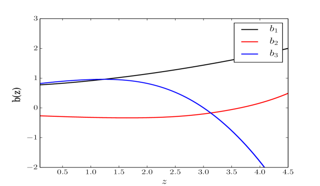
Figure 5: The HI bias parameters used in the paper.

References

(1)
P. Bull, P. G. Ferreira, P. Patel and M. G. Santos,
Astrophys. J. 803, 21 (2015)
[arXiv:1405.1452 [astro-ph.CO]].
(2)
A. Hall, C. Bonvin and A. Challinor,
Phys. Rev. D 87, 064026 (2013)
[arXiv:1212.0728 [astro-ph.CO]].
(3)
S. Camera, M. G. Santos, P. G. Ferreira and L. Ferramacho,
Phys. Rev. Lett. 111, 171302 (2013)
[arXiv:1305.6928 [astro-ph.CO]].
(4)
M. G. Santos et al.,
arXiv:1501.03989 [astro-ph.CO].
(5)
D. Alonso, P. Bull, P. G. Ferreira, R. Maartens and M. G. Santos,
arXiv:1505.07596 [astro-ph.CO].
(6)
A. Raccanelli, F. Montanari, D. Bertacca, O. Doré and R. Durrer,
arXiv:1505.06179 [astro-ph.CO].
(7)
D. Alonso and P. G. Ferreira,
arXiv:1507.03550 [astro-ph.CO].
(8)
J. Fonseca, S. Camera, M. Santos and R. Maartens,
arXiv:1507.04605 [astro-ph.CO].
(9)
T. Baker and P. Bull,
arXiv:1506.00641 [astro-ph.CO].
(10)
R. E. Smith et al. [VIRGO Consortium Collaboration],
Mon. Not. Roy. Astron. Soc. 341, 1311 (2003)
[astro-ph/0207664].
(11)
A. F. Heavens, S. Matarrese and L. Verde,
Mon. Not. Roy. Astron. Soc. 301, 797 (1998)
[astro-ph/9808016].
(12)
P. McDonald,
Phys. Rev. D 74, 103512 (2006)
[Phys. Rev. D 74, 129901 (2006)]
[astro-ph/0609413].
(13)
P. McDonald and A. Roy,
JCAP 0908, 020 (2009)
[arXiv:0902.0991 [astro-ph.CO]].
(14)
K. C. Chan and R. Scoccimarro,
Phys. Rev. D 86, 103519 (2012)
[arXiv:1204.5770 [astro-ph.CO]].
(15)
A. J. Nishizawa, M. Takada and T. Nishimichi,
Mon. Not. Roy. Astron. Soc. 433, 209 (2013)
[arXiv:1212.4025 [astro-ph.CO]].
(16)
V. Assassi, D. Baumann, D. Green and M. Zaldarriaga,
JCAP 1408, 056 (2014)
[arXiv:1402.5916 [astro-ph.CO]].
(17)
P. A. R. Ade et al. [Planck Collaboration],
arXiv:1502.01589 [astro-ph.CO].
(18)
D. Bertacca, R. Maartens and C. Clarkson,
JCAP 1409, 037 (2014)
[arXiv:1405.4403 [astro-ph.CO]].
(19)
D. Bertacca, R. Maartens and C. Clarkson,
JCAP 1411, 013 (2014)
[arXiv:1406.0319 [astro-ph.CO]].
(20)
J. Yoo and M. Zaldarriaga,
Phys. Rev. D 90, 023513 (2014)
[arXiv:1406.4140 [astro-ph.CO]].
(21)
E. Di Dio, R. Durrer, G. Marozzi and F. Montanari,
JCAP 1412, 017 (2014)
[JCAP 1506, no. 06, E01 (2015)]
[arXiv:1407.0376 [astro-ph.CO]].
(22)
D. Bertacca,
arXiv:1409.2024 [astro-ph.CO].
(23)
O. Umeh, C. Clarkson and R. Maartens,
Class. Quantum Grav. 31, 202001 (2014)
[arXiv:1207.2109 [astro-ph.CO]].
(24)
O. Umeh, C. Clarkson and R. Maartens,
Class. Quant. Grav. 31, 205001 (2014)
[arXiv:1402.1933 [astro-ph.CO]].