Sculpting a quasi-one-dimensional Bose-Einstein condensate to generate calibrated matter-waves

Abstract

We explore theoretically how to tune the dynamics of a quasi one-dimensional harmonically trapped Bose-Einstein condensate (BEC) due to an additional red- and blue-detuned Hermite-Gaussian dimple trap (HGdT). To this end we study a BEC in a highly non-equilibrium state, which is not possible in a traditional harmonically confined trap. Our system is modeled by a time-dependent Gross-Pitaevskii equation, which is numerically solved by the Crank-Nicolson method in both imaginary and real time. For equilibrium, we obtain a condensate with two bumps/dips which are induced by the chosen TEM₀₁ mode for the red/blue-detuned HGdT, respectively. Afterwards, in time-of-flight dynamics, we examine the adherence/decay of the two bumps/dips in the condensate, which are induced by the still present red/blue-detuned HGdT, respectively. On the other hand, once the red/blue HGdT potential is switched off, shock-waves or bi-trains of gray/dark pair-solitons are created. During this process it is found that the generation of gray/dark pair-solitons bi-trains are generic phenomena of collisions of moderately/fully fragmented BEC. Additionally, it turns out that the special shape of generated solitons in the harmonically trapped BEC firmly depends upon the geometry of the HGdT.

I Introduction

The development of laser cooling has accelerated a tremendous interest in the confinement and manipulation of cold atoms. In particular, using optical dipole traps generated by red/blue-detuned resonance laser light has become a versatile tool for the manipulation of atoms. Recently, optical dipole traps created by a red-detuned laser beam have become common, experimentally Stamper-Kurn et al. (1998); Madison et al. (2000, 2001); Barrett et al. (2001); Gustavson et al. (2001); Hammes et al. (2002); Comparat et al. (2006); Scherer et al. (2007); Schulz et al. (2007); Tuchendler et al. (2008); Jacob et al. (2011); Garrett et al. (2011) as well as theoretically Diener et al. (2002); Proukakis et al. (2006); Carpentier et al. (2008); Aioi et al. (2011); Uncu et al. (2011); Weitenberg et al. (2011); Akram and Pelster (2015), they are known as a “tweezer” or “dimple-trap” provided that the trap is quite sharp. Red-detuned dimple traps have become important tools for BEC production Stamper-Kurn et al. (1998); Barrett et al. (2001); Jacob et al. (2011), transport of a BEC over long distances Gustavson et al. (2001), and formation of shock-waves in harmonic plus a dimple trap Akram and Pelster (2015). Blue-detuned optical dipole traps, instead, are mostly used as a repulsive obstacle for atoms Raman et al. (1999); Onofrio et al. (2000); Raman et al. (2001); Neely et al. (2010); Akram and Pelster (2015). The HG laser beams are higher order solutions of the paraxial wave equation with rectangular symmetry about their axes of propagation Saleh and Teich (2007); Milonni and Eberly (2010). Due to their enormous application areas, there have been several attempts to develop such higher order beam modes Kozawa and Sato (2005); Flores-Pérez et al. (2006); Novitsky and Barkovsky (2006). For example, the resonator of a laser is manipulated such that the beam is emitted in a desired beam mode structure Mushiake et al. (1972), or transforms a general Gaussian laser-beam with interferometric methods into the desired modes Dorn et al. (2003); Török and Munro (2004); Toussaint et al. (2005). These interferometric methods are typically based on the addition or subtraction of different scalar laser beam modes Tidwell et al. (1993). To switch between different modes, a more flexible way is to use a spatial light modulator to generate the desired higher order laser modes Stalder and Schadt (1996); Neil et al. (2002). It is already known that HG laser modes possess interesting properties, however, to the best of our knowledge, so far only two experimental papers have been published about the confinement of atoms in higher order optical dipole traps Meyrath et al. (2005); Smith et al. (2005).

In this paper, we consider a theoretical analysis of a quasi one-dimensional (1D) Bose-Einstein condensate confined by both a harmonic trap and a Hermite-Gaussian dimple trap (HGdT). The red/blue-detuned HGdT can be generated by using the Hermite-Gaussian (HG) laser beam. The mean-field description of the one-dimensional macroscopic BEC wave function is based upon the Gross-Pitaevskii equation Pitaevskii and Stringari (2003); Pethick and Smith (2008); Kevrekidis et al. (2008). A truly 1D mean-field regime, also known as Tonks-Girardeau regime, requires transverse dimensions of the trap on the order of or less than the atomic s-wave scattering length Olshanii (1998); Petrov et al. (2000); Bergeman et al. (2003). In contrast, the quasi one-dimensional regime of the Gross-Pitaevskii equation holds when the transverse dimension of the trap is larger than or of the order of the s-wave scattering length and much smaller than the longitudinal extension Pérez-García et al. (1998); Jackson et al. (1998); Carr et al. (2000a, b); Adhikari (2006). Here we focus our attention to a quasi one-dimensional Gross-Pitaevskii equation (1DGPE). This regime is quite interesting, as it is well-known to feature bright solitons for attractive s-wave scattering lengths Strecker et al. (2003); Abdullaev et al. (2004); Herring et al. (2005); C. Becker et al. (2008), gray/dark solitons for repulsive s-wave scattering lengths Denschlag et al. (2000); Huang et al. (2002); Radouani (2004); Yan et al. (2012); Hans et al. (2015) or the formation of shock waves in a BEC Chang et al. (2008); Meppelink et al. (2009).

With this, we organize our paper as follows. We derive the underlying quasi one-dimensional Gross-Pitaevskii equation (1DGPE) in Sec. 1, where, we also outline the system geometry and relate our simulation parameters to tunable experimental parameters. Afterwards in Sec. III, for the equilibrium properties of the system, we compare a Thomas-Fermi approximate solution with numerical results and show that the HGdT imprint upon the condensate wave function strongly depends upon whether the HGdT is red or blue-detuned. Later, in Sec. IV we assume that the magnetic trap is switched off and we determine the time-of-flight (TOF) dynamics of the condensate wave function, when the HGdT is still present. On the one hand we obtain that for red-detuning the HGdT imprint does not decay, but for the blue-detuning the HGdT imprint decreases during TOF. On the other hand, we discuss in detail how the collision of the condensate with the HGdT potential during the non-ballistic expansion leads to characteristic matter-wave stripes. In Sec. V, we investigate instead matter-wave interferences in form of the formation of shock-waves/gray(dark) pair-soliton bi-trains in the harmonic trap, after having switched off the red/blue-detuned HGdT potential. There, we also find out that the generation of gray/dark pair-solitons bi-trains represents a generic phenomenon of collisions of moderately/fully fragmented BEC, which strongly depends upon the equilibrium values of the red/blue-detuned HGdT depth. Finally, Sec. VI provides a summary and conclusions.

II modified quasi 1D model

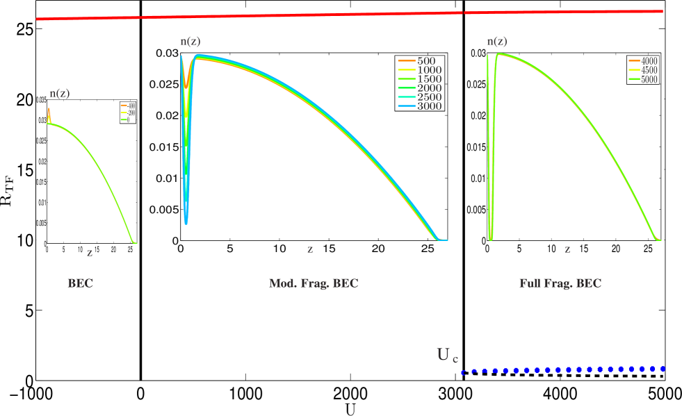
Figure 1: (Color online) Outer Thomas-Fermi radius $\text{R}_{\text{TF1}}$ (red solid), central Thomas-Fermi radius $\text{R}_{\text{TF2}}$ (blue dashed) and inner Thomas-Fermi radius $\text{R}_{\text{TF3}}$ (dotted black) as a function of HGdT depth $U$ in dimensionless units for the coupling constant value $G_{\text{B}}=11435.9$. Below the critical value HGdT depth $U<U_{\text{c}}$, the BEC is moderately (Mod.) fragmented (Frag.), with one exceptional case at $U=0$, where the BEC is completely confined in one-dimensional harmonic trap. The BEC fully fragments into three parts above the critical value $U_{\text{c}}\approx 3079$, as can be seen in the specific regional inset density plots.

We consider a one-component BEC with time-dependent two-particle interactions described by the three-dimensional GPE

$$i\hbar\frac{\partial}{\partial t}\psi\left(\mathbf{r},t\right)=\left\{-\frac{\hbar^{2}}{2m_{B}}\nabla^{2}+V(\mathbf{r})+U_{\text{dT}}^{\text{3D}}\right.$$ (1)

$$\left.+G_{\text{B}}^{\text{3D}}\parallel\psi\left(\mathbf{r},t\right)\parallel^{2}\right\}\psi\left(\mathbf{r},t\right),$$

where $\psi\left(\mathbf{r},t\right)$ denotes the macroscopic condensate wave function for the ${}^{87}\text{Rb}$ BEC with the spatial coordinates $\mathbf{r}=\left(x,\;y,\;z\right)$. Here $m_{\text{B}}$ stands for the mass of the ${}^{87}\text{Rb}$ atom, $G_{\text{B}}^{\text{3D}}=N_{\text{B}}4\pi\hbar^{2}a_{\text{B}}/m_{\text{B}}$ represents the three-dimensional ${}^{87}\text{Rb}$ coupling constant, where $N_{\text{B}}=20\times 10^{4}$ denotes the number of ${}^{87}\text{Rb}$ atoms, and the s-wave scattering length is $a_{\text{B}}=94.7~{}{\rm{a}_{0}}$ with the Bohr radius ${\rm{a}_{0}}$. Furthermore, $V\left(\mathbf{r}\right)=m_{\text{B}}\omega_{\text{z}}^{2}z^{2}/2+m_{\text{B}}\omega_{\text{r}}^{2}\left(x^{2}+y^{2}\right)/2$ describes a three-dimensional harmonic confinement, which has rotational symmetry with respect to the $z$-axis. The oscillator lengths for experimental parameters are $l_{\text{z}}=\sqrt{\hbar/m_{\text{B}}\omega_{\text{z}}}=4.12\,\mu\text{m}$ and $l_{\text{r}}=\sqrt{\hbar/m_{\text{B}}\omega_{\text{r}}}=0.84\,\mu\text{m}$ for the trap frequencies $\omega_{\text{z}}=2\pi\times 6.8\,\text{Hz}$ and $\omega_{\text{r}}=2\pi\times 160\,\text{Hz}$, respectively.

An additional three-dimensional narrow Hermite-Gaussian laser beam polarizes the neutral atoms which yields the HGdT potential $U_{\text{dT}}^{\text{3D}}=U_{\text{0}}\text{I}_{nm}\left(\mathbf{r}\right)$. Within the rotating-wave approximation its amplitude is $U_{\text{0}}=3\pi c^{2}\Gamma/\left(2\omega_{\text{A}}^{3}\Delta\right)$ Allen and Eberly (1987); Scully and Zubairy (1997); Saleh and Teich (2007); Milonni and Eberly (2010), where $\Gamma=\left|<e|{\bf d}|g>\right|^{2}\omega_{\text{A}}^{3}/\left(3\pi\epsilon_{0}\hbar c^{3}\right)$ denotes the damping rate due to energy loss via radiation, which is detected by the dipole matrix element between ground and excited state. Furthermore, $\Delta=\omega-\omega_{\text{A}}$ represents the detuning of the laser, here $\omega$ is the laser frequency and $\omega_{\text{A}}$ stands for the atomic frequency. And $\text{I}_{nm}\left(\mathbf{r}\right)$ describes the intensity profile of the TEM_nm Hermite-Gaussian laser beam, which is assumed to propagate in $y$-direction and is determined via

$$\text{I}_{nm}\left(\mathbf{r}\right)= \frac{2P}{2^{n+m}n!m!\pi}H_{n}\left(\frac{\sqrt{2}x}{W_{\text{x}}\left(y\right)}\right)^{2}H_{m}\left(\frac{\sqrt{2}z}{W_{\text{z}}\left(y\right)}\right)^{2}$$

$$\times\frac{e^{-\left[\frac{2x^{2}}{W_{\text{x}}^{2}\left(y\right)}+\frac{2z^{2}}{W_{\text{z}}^{2}\left(y\right)}\right]}}{W_{\text{x}}\left(y\right)W_{\text{z}}\left(y\right)}\,,$$

with $P=\int\int\text{I}_{nm}\left(\mathbf{r}\right)dxdz$ being the normalization constant. Furthermore $W_{\text{x/z}}^{2}(y)=W_{\text{0x/z}}^{2}\left(1+y^{2}/y_{\text{Rx/z}}^{2}\right)$ denotes the Gaussian beam radius in the $x$- and $z$-direction, where the intensity decreases to $1/e^{2}$ of its peak value, $y_{Rx/z}=\pi W_{0x/z}^{2}/\lambda$ represents the so-called Rayleigh-lengths, which are defined as the distance from the focus $W_{\text{0x/z}}$ position where the beam radius increases by a factor of $\sqrt{2}$ Saleh and Teich (2007). Here $H_{n}\left(q\right)$ and $H_{m}\left(q\right)$ are Hermite polynomials of order $n$ and $m$ in $x$- and $z$-directions, respectively. In the following we restrict ourselves to a HGdT potential for a BEC, which is based on a Hermite-Gaussian TEM₀₁ laser beam mode and thus carries a dark spot in the center of the profile:

$$\text{I}_{01}\left(\mathbf{r}\right)=\frac{8Pz^{2}}{\pi W_{\text{x}}\left(y\right)W_{\text{z}}^{3}\left(y\right)}e^{-\left[\frac{2x^{2}}{W_{\text{x}}^{2}\left(y\right)}+\frac{2z^{2}}{W_{\text{z}}^{2}\left(y\right)}\right]}\,.$$ (3)

For the TEM₀₁ laser beam, we use the width along the $x$-axis $W_{\text{0x}}=1.1\,\mu\text{m}$ and along the $z$-axis $W_{\text{0z}}=3.2\,\mu\text{m}$. Therefore, the Rayleigh lengths for the red-detuned laser light with $\lambda=840\,\text{nm}$ Garrett et al. (2011) yield $y_{\text{Rx}}=4.526\,\mu\text{m}$ and $y_{\text{Rz}}=38.29\,\mu\text{m}$ as well as for the blue detuned laser light with $\lambda=772\,\text{nm}$ Xu et al. (2010) we get $y_{\text{Rx}}=4.92\,\mu\text{m}$ and $y_{\text{Rz}}=41.6\,\mu\text{m}$. With keeping in mind the fact $y_{\text{Rx}/\text{z}}\gg l_{\text{r}}$, we can approximate the widths of the HG laser beam in $x$- and $z$-direction according to $W_{\text{x}/\text{z}}(y)\approx W_{0\text{x}/\text{z}}$. This simplifies the HGdT potential to

$$U_{\text{dT}}^{\text{3D}}\left(\mathbf{r}\right) =\frac{8U_{0}Pz^{2}}{\pi W_{\text{0x}}W_{\text{0z}}^{3}}e^{-\left(\frac{2x^{2}}{W_{0\text{x}}^{2}}+\frac{2z^{2}}{W_{0\text{z}}^{2}}\right)}.$$ (4)

As we have an effective one-dimensional setting due to $\omega_{\text{z}}\ll\omega_{\text{r}}$, which implies $l_{\text{z}}>l_{\text{r}}$, and $y_{\text{Rx}/\text{z}}\gg l_{\text{r}}$, we factorize the BEC wave-function via $\psi(\mathbf{r},t)=\psi(z,t)\phi(r_{\perp},t)$ with ${\bf r}_{\perp}=\left(x,\;y\right)$ and

$$\phi({\bf r}_{\perp},t) = \frac{e^{-\frac{x^{2}+y^{2}}{2l_{\text{r}}^{2}}}}{\sqrt{\pi}l_{\text{r}}}e^{-i\omega_{\text{r}}t}\,.$$ (5)

We follow Ref. Kamchatnov (2004) and integrate out the two transversal dimensions of the three-dimensional GPE. After some algebra, the resulting quasi one-dimensional GPE reads

$$i\hbar\frac{\partial}{\partial t}\psi\left(z,t\right)=\left\{-\frac{\hbar^{2}}{2m_{B}}\frac{\partial^{2}}{\partial z^{2}}+V\left(z\right)+Uz^{2}e^{-\frac{2z^{2}}{W_{\text{0z}}^{2}}}\right.$$ (6)

$$\left.+G_{\text{B}}\parallel\psi\left(z,t\right)\parallel^{2}\right\}\psi\left(z,t\right),$$

where $V\left(z\right)=m_{\text{B}}\omega_{z}^{2}z^{2}/2$ represents an effective one-dimensional harmonic potential from the MOT, and the one-dimensional two-particle interaction strength turns out to be

$$G_{\text{B}}=2N_{\text{B}}a_{\text{B}}\hbar\omega_{\text{r}}\,.$$ (7)

Furthermore, the one-dimensional HGdT depth results in

$$U=\frac{8U_{0}P}{\pi W_{\text{0z}}^{3}\sqrt{W_{\text{0x}}^{2}+2l_{\text{r}}^{2}}}\,,$$ (8)

In order to make the 1DGPE in (6) dimensionless, we introduce the dimensionless time as $\tilde{t}=\omega_{\text{z}}t$, the dimensionless coordinate $\tilde{z}=z/l_{\text{z}}$, and the dimensionless wave function $\tilde{\psi}=\psi\sqrt{l_{\text{z}}}$. With this Eq. (6) can be written in dimensionless form

$$i\frac{\partial}{\partial\tilde{t}}\tilde{\psi}\left(\tilde{z},\tilde{t}\right)=\left\{-\frac{1}{2}\frac{\partial^{2}}{\partial\tilde{z}^{2}}+\frac{1}{2}\tilde{z}^{2}+\tilde{U}\tilde{z}^{2}e^{-\frac{\tilde{z}^{2}}{\tilde{\alpha}^{2}}}\right.$$ (9)

$$\left.+\tilde{G}_{\text{B}}\parallel\tilde{\psi}\left(\tilde{z},\tilde{t}\right)\parallel^{2}\right\}\tilde{\psi}\left(\tilde{z},\tilde{t}\right),$$

here $\tilde{G}_{\text{B}}=2N_{\text{B}}\omega_{\text{r}}a_{\text{B}}/\omega_{\text{z}}l_{\text{z}}$, and $\tilde{U}=8U_{0}Pl_{\text{z}}/\left(\pi\omega_{\text{z}}W_{\text{0z}}^{3}\sqrt{W_{\text{0x}}^{2}+2l_{\text{r}}^{2}}\right)$ are the dimensionless two-particle coupling strength and the dimensionless HGdT depth, respectively. The above mentioned experimental values yield the dimensionless Rb-Rb coupling constant $\tilde{G}_{\text{B}}=11435.9$ and $\tilde{\alpha}=W_{\text{0z}}/\left(\sqrt{2}l_{\text{z}}\right)=0.548$ represents the ratio of the width of the HGdT potential and the harmonic oscillator length along the $z$-axis. Furthermore, the typical depth of dipole potential traps ranges from micro-kelvin to nano-kelvin Bongs and Sengstock (2004); Yin (2006), which yields $\tilde{U}$ to be of the order of up to few thousands. From here on, we will drop all tildes for simplicity.

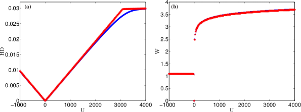
Figure 2: (Color online) (a) Height/depth and (b) width of red/blue-detuned HGdT induced bumps/dips according to Eq. (13) and $\text{W}=2z_{\text{Max}}$, respectively, versus red/blue-detuned HGdT depth $U$ in dimensionless units for the experimental BEC coupling constant $G_{\text{B}}=11435.9$ determined numerically by solving the quasi 1DGPE (9) in dimensionless imaginary time (blue circles) and analytically (red stars) from the BEC TF wave function (10).

III Stationary Condensate Wave Function

In order to determine the equilibrium properties of the red/blue-detuned HGdT potential imprint on the condensate wave function, we solve the quasi 1DGPE (9) numerically by using the split-operator method in imaginary time Vudragović et al. (2012); Kumar et al. (2015); Lončar et al. (2016); Satarić et al. (2016). The HGdT imprint induces two bumps/dips at the center of the BEC density for red/blue-detuned HGdT as shown in the insets of Fig. 1. For stronger red-detuned HGdT depth values the two bumps increase further, but for stronger blue-detuned HGdT depth the two dips in the BEC density get deeper and deeper until the BEC fragments into three parts as shown in the inset of Fig. 1. To investigate this scenario in more detail, we argue that, due to $G_{\text{B}}\gg 1$, the TF approximation is valid, as the inequality ${\rm E_{\text{{\rm int,pot}}}/E_{\text{{\rm kin}}}\gg 1}$ holds within the whole region of interest for the HGdT depth $U$ Akram and Pelster (2015).

Therefore we perform for the condensate wave function the ansatz $\psi(z,t)=\psi(z)e^{-i\mu t}$, insert it into the modified quasi 1DGPE (9), and neglect the kinetic energy term, yielding the density profile

$$\psi\left(z\right)=\sqrt{\frac{\mu}{G_{\text{B}}}\left(1-\frac{z^{2}}{2\mu}-\frac{Uz^{2}}{\mu}e^{-\frac{z^{2}}{\alpha^{2}}}\right)}$$ (10)

$$\times\Theta\left(1-\frac{z^{2}}{2\mu}-\frac{Uz^{2}}{\mu}e^{-\frac{z^{2}}{\alpha^{2}}}\right)\,.$$

In view of the normalization $2\intop_{0}^{\infty}\parallel\psi\left(z\right)\parallel^{2}dz=1$, which fixes the chemical potential $\mu$, we determine the Thomas-Fermi radii $\text{R}_{\text{TF}}$ from the condition that the condensate wave function vanishes:

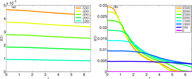
Figure 3: (Color online) Height/depth versus dimensionless time during TOF for different (a) red-detuned and (b) blue-detuned HGdT depths $U$ in dimensionless units.

Figure 4: (Color online) Time-of-flight evolution of depleted density $\parallel\psi\left(z,t\right)\parallel_{\text{DD}}^{2}=\parallel\psi\left(z,t\right)\parallel_{U\neq 0}^{2}-\break\parallel\psi\left(z,t\right)\parallel_{U=0}^{2}$ from solving the modified quasi 1DGPE equation for different values of $|U|$: (a) $U=-500$, (b) $U=1500$, (c) $U=2500$, and (d) $U=3500$ in dimensionless units.

$$\mu=\frac{\text{R}_{\text{TF}}^{2}}{2}+U\text{R}_{\text{TF}}^{2}e^{-\frac{\text{R}_{\text{TF}}^{2}}{\alpha^{2}}}\,.$$ (11)

As can be read off from the inset of the Fig. 1 the number of solutions of Eq. (10) changes for increasing red/blue-detuned HGdT depth U. In the case, when $U$ is smaller than $U_{\text{c}}$, Eq. (10) defines only the BEC cloud radius $\text{R}_{\text{TF1}}$. But for the case $U>U_{\text{c}}$, the blue-detuned HGdT drills two holes at the center of the ${}^{87}\text{Rb}$ condensate, so the BEC fragments into three parts as shown in Fig. 1. Thus, we have then, apart from the outer condensate radius $\text{R}_{\text{TF1}}$, also two inner condensate radii $\text{R}_{\text{TF2}}$ and $\text{R}_{\text{TF3}}$. With this the normalization condition $2\intop_{0}^{\text{R}_{\text{TF3}}}\parallel\psi\left(z\right)\parallel^{2}dz+2\intop_{\text{R}_{\text{TF2}}}^{\text{R}_{\text{TF1}}}\parallel\psi\left(z\right)\parallel^{2}dz=1$ yields

$$\mu\left(\text{R}_{\text{TF1}}-\text{R}_{\text{TF2}}+\text{R}_{\text{TF3}}\right)-\frac{1}{6}\left(\text{R}_{\text{TF1}}^{3}-\text{R}_{\text{TF2}}^{3}+\text{R}_{\text{TF3}}^{3}\right)\,\,\,$$ (12)

$$+\frac{\alpha^{2}U}{2}\left(\text{R}_{\text{TF1}}e^{-\frac{\text{R}_{\text{TF1}}^{2}}{\alpha^{2}}}-\text{R}_{\text{TF2}}e^{-\frac{\text{R}_{\text{TF2}}^{2}}{\alpha^{2}}}+\text{R}_{\text{TF3}}e^{-\frac{\text{R}_{\text{TF3}}^{2}}{\alpha^{2}}}\right)=$$

$$\frac{\alpha^{3}\sqrt{\pi}U}{4}\left[\text{Erf}\left(\frac{\text{R}_{\text{TF1}}}{\alpha}\right)-\text{Erf}\left(\frac{\text{R}_{\text{TF2}}}{\alpha}\right)+\text{Erf}\left(\frac{\text{R}_{\text{TF3}}}{\alpha}\right)\right]\,,$$

where $\text{Erf}(y)=\frac{2}{\sqrt{\pi}}\int_{0}^{y}e^{-x^{2}}dx$ denotes the error function. In case of $U<U_{\text{c}}$, the BEC’s inner two radii $\text{R}_{\text{TF2}}$ and $\text{R}_{\text{TF3}}$ vanish and the BEC outer radius is approximated via $\text{R}_{\text{TF1}}\approx\sqrt{2\mu}$ due to Eq. (11). Thus, for $U<U_{\text{c}}$ the BEC chemical potential is determined explicitly from (12): $\mu\approx 3^{2/3}/2^{7/2}\left(2G_{\text{B}}+\sqrt{\pi}\alpha^{3}U\right)^{2/3}$. Provided that $U>U_{\text{c}}$, two inner cloud radii $\text{R}_{\text{TF2}}$ and $\text{R}_{\text{TF3}}$ have to be taken into account according to Fig. 1. We observe that the Thomas-Fermi value of the critical red/blue-detuned HGdT depth $U_{\text{c}}\approx 3079$ is close to the numerical one $U_{\text{c}}\approx 3090$. Figure 1 also shows the resulting outer and inner Thomas-Fermi radius as a function of the red/blue-detuned HGdT depth U. Here, the two inner radii behave symmetric, e.g., for $U>3079$ the $\text{R}_{\text{TF2}}$ is increasing and $\text{R}_{\text{TF3}}$ is decreasing correspondingly, however after $U\gtrsim 4500$, they both become approximately constant as shown in Fig. 1. We also read off that $\text{R}_{\text{TF1}}\approx\sqrt{2\mu}$ remains approximately constant for $U>U_{\text{c}}$, so we conclude that the chemical potential $\mu$ is then sealed to its critical value $\mu_{c}\approx 341.28$.

In the perspective of a quantitative comparison between the analytical and the numerical calculation, we characterize the red/blue-detuned HGdT induced imprint upon the condensate wave function by the following two quantities. The first one is the red/blue-detuned HGdT induced imprint height/depth

$$\begin{array}[]{r@{}l@{\,}l}\text{HD}=\left\{\begin{array}[]{r@{}l@{\,}l}\text{Max}\left(\parallel\Psi\left(z\right)\parallel^{2}\right)-\parallel\Psi\left(0\right)\parallel^{2}\quad U\leq 0\vspace{5mm}\\ \parallel\Psi\left(0\right)\parallel^{2}-\text{Min}\left(\parallel\Psi\left(z\right)\parallel_{z\rightarrow 0}^{2}\right)\quad U>0\end{array}\right.\end{array}$$ (16)

and the second one is the red/blue-detuned HGdT induced imprint width $\text{W}=2z_{\text{Max}},$ where $z_{\text{Max}}$ denotes the coordinate of maximal density. To find out a one-to-one resemblance between analytical and numerical calculation of HD and W, we determine the solution of the dimensionless 1DGPE (9) and compare it with the TF solution of Eq. (10), as shown in Fig. 2. The case $U=0$, i.e., when the HGdT potential is switched off, corresponds to a BEC in a quasi one-dimensional harmonic trap. Furthermore, in the range $U<U_{\text{c}}$ we observe that the red/blue-detuned HGdT induced imprint height/depth changes linearly with the optical dipole trap depth $U$ according to

$$\text{HD}\approx\frac{\alpha^{2}|U|e^{T\left(-e/2|U|\right)-1}}{G_{\text{B}}}\, U\neq 0\,,\alpha\neq 0\,,$$ (17)

where $T=xe^{x}$ abbreviates the productlog function. In case of $U>U_{\text{c}}$ the blue-detuned HGdT induced imprint depth yields the constant value $\text{\text{HD}}_{\text{c}}\approx 0.0296$ as follows from Eq. (17), which slightly deviates from the corresponding numerical value $\text{\text{HD}}_{\text{c}}=0.027$. Similarly, the red/blue-detuned HGdT induced imprint width follows from $\text{W}=2\alpha\sqrt{1-T\left(-e/2|U|\right)}$ according to the TF approximation, which reduces at the critical blue-detuned optical dipole depth to $\text{W}_{\text{c}}\approx 3.60$ whereas the corresponding numerical value is $\text{W}_{\text{c}}\approx 3.64$, as shown in Fig. 2.

IV Time-of-Flight dynamics of red/blue-detuned HGdT induced imprint

The time-of-flight (TOF) expansion has been used to measure various BEC properties since the field’s inception. By suddenly turning off the magnetic trap, when the HGdT is still present, the atom cloud is allowed to expand in all directions. This expansion proceeds according to the momenta of the atoms at the initial time $t=0$ and an additional tiny acceleration results from inter-particle interactions. The red-detuned HGdT induced two bumps remain approximately constant during the temporal evolution as shown in Fig. 3(a). But the blue-detuned HGdT induced two dips at the center of the condensate start decaying with a characteristic time scale after having switched off the trap as shown in Fig. 3(b). Furthermore, the dips of the HGdT induced imprint start decaying faster with increasing blue-detuned HGdT depth for smaller time as shown in Fig. 3(b). Note that the relative speed of the bumps or dips from each other turns out to vanish.

Furthermore, we investigate in detail the possible occurrence of matter-wave stripes at the top of the condensate during the non-ballistic expansion of the moderately/fully fragmented BEC cloud by plotting the density distribution of the released cloud correspondingly as shown in Fig. 4. According to Fig. 4(a) we do not observe any particular structure for the red-detuned HGdT induced imprint, but Fig. 4(b-d) shows for the blue-detuned HGdT induced imprint that characteristic matter-wave stripes occur, which are generated, while the freely expanding BEC collides with the HGdT potential. For small blue-detuned HGdT depth, the generation of matter-wave stripes can be seen at later time, as compared to higher blue-detuned HGdT depth, as shown in Fig. 4(b-d). The matter-wave stripes are directly visible for $U<U_{\text{c}}$, as can be explained as follows. In Fig. 4(b), the height of the blue-detuned HGdT induced two dips is smaller as compared to Fig. 4(c), therefore they need more time to drill a hole in the condensate during TOF. For the HGdT potential depth $U=1500$, the BEC fragments into three parts at the dimensionless time $t=2.4$, afterwards the three fragmented condensates start to interact as separate identities with the HGdT potential, which leads to the formation of characteristic matter-wave stripes. The similar phenomenon happens in Fig. 4(c), but in this example the initial HGdT potential depth $U=2500$ is larger than the previous one in Fig. 4(b), so the BEC becomes fragmented at the earlier time $t=1.3$. In the example of Fig. 4(d), when $U>U_{\text{c}}$, the BEC is already initially, i.e. at time $t=0$, fragmented according to Fig. 1. Therefore the matter-wave stripes can be seen just after $t>0$, but the stripes are not as visible as in the two previous cases.

Figure 5: (Color online) Coherent matter-waves evolution in the BEC density, when red/blue-detuned HGdT potential is switched off, versus time and position for different values of (a) $U=-500$, (b) $U=1500$, (c) $U=2500$, and (d) $U=3500$. Graphs (e-h) show the BEC density at time $t=5.3$, and in graphs (i-l) we plotted the corresponding energies $E(t)=E(t)/\text{Max}(E(t))$ versus time for the HGdT depths $U$ of the graphs (a-d) in dimensionless units.

V Shock-waves and gray/dark pair-solitons bi-trains

In this section, we show that matter-wave self-interferences emerge, once the red/blue-detuned HGdT potential is suddenly switched off, within the remaining harmonic confinement, as this leads to shock waves and gray/dark pair-solitons bi-trains, respectively as shown in Fig. 5(a-d). A shock-wave is a special kind of propagating disturbance in the BEC, whose amplitude, unlike for solitons, decreases relatively quickly with large distance. Furthermore, gray/dark solitons have a characteristic property that they can pass through one another without any change of shape, amplitude, or speed. We can see from Fig. 5(b-d) that the pair-solitons bi-trains do, indeed, pass through one another and that they are reflected from the end of the trapping potential.

Once the red/blue-detuned HGdT potential is switched off, the system quasi-instantaneously adjusts its energy to the new equilibrium, paving the way for the creation of shock-waves and bi-trains of gray/dark pair-solitons, respectively. The total normalized energy ${\rm E({\rm t)={\rm E(t)/\text{Max}({\rm E(t))}}}}$ as shown in Fig. 5(i-l), changes quite quickly from its initial value to a new equilibrium value, thus generating the shock-waves or the pair-solitons bi-trains. For an initial red- and blue-detuned HGdT depth, we observe that two excitations of the condensate are created at the position of the red/blue-detuned HGdT potential, which travel in the opposite direction with the same center-of-mass speed, are reflected back from the harmonic trap boundaries, and then collide at the red/blue-detuned HGdT potential position as shown in Fig. 5(a-d).

We have performed calculations for different red-detuned HGdT potential depths $U<0$ and in all cases we observe the formation of the shock-wave structures as shown in Fig. 5(a). The density of atoms around the shocks is mostly enhanced in comparison with the density far away from these perturbations. And for the blue-detuned HGdT potential trap, we detect gray/dark pair-solitons bi-trains, traveling in opposite directions with the same speed as shown in Fig. 5(b-d). The creation of these calibrated gray/dark pair-solitonic bi-trains are generic collision phenomena of moderately/fully fragmented BEC, which is strongly depending upon the equilibrium values of the red/blue-detuned HGdT potential depth, respectively.

The dynamics of one gray/dark soliton in a BEC cloud is well described by $\ddot{z}=-(1/2)\partial V_{\text{ext}}/\partial z$, where $V_{\text{ext}}$ is the dimensionless confining potential and $z$ denotes the position of the gray/dark soliton. In the case of harmonic confinement with a potential $V_{\text{ext}}=z^{2}/2$ the solution of this evolution equation leads to an oscillation of the soliton described by $z(t)=\text{R}_{\text{TF1}}\sin\left(t/\sqrt{2}\right)$. Thus the frequency of the oscillating soliton and the frequency of the dipole oscillation of the Bose-Einstein condensate in the trap differ by the factor $\sqrt{2}$ Busch and Anglin (2001). In our system, pair-solitons bi-trains generally oscillate with the average frequency $\Omega=2\pi\times 4.80~{}{\rm Hz}$ irrespective of the sign and the size of $U$ as shown in Fig. 5. With this, we get the ratio $\Omega/\omega_{{\rm z}}\approx 0.705$, which is quite close to the dimensionless soliton frequency $1/\sqrt{2}\approx 0.707$ in a harmonic trap as predicted in Ref. Busch and Anglin (2001). Note that previously the generation of solitons was studied theoretically by investigating the collision of two condensates Scott et al. (1998) and experimentally for different quasi one-dimensional trap geometries Weller et al. (2008); Shomroni et al. (2009). Although in the latter experiments only one potential maximum occurs instead of two as in our work, so there single solitons and here pairs of solitons are observed, the basic physics is the same.

We also observe an intriguing substructure of each soliton, which we call pair-soliton. Normally, we find that there are solitons which always move in pairs, and the mean distance between each other is less than the neighboring solitons as shown in Fig. 5(b-d) and Fig. 5(f-h). Numerically, we have observed that the averaged distance between pair-solitons is less for dark solitons as compared to the gray solitons as shown in Fig. 5(f-h). We also observe that, in general, a minimal time of about $4.6\,$ms is required to generate shock-waves/pair-solitons bi-trains as shown in Fig. 5. The number of shock-waves is not effected by the red/blue-detuned HGdT potential depth, but the number of interference fringes increases. On the other hand, we observe that the number of gray/dark pair-solitons depends on the depth of the red/blue-detuned HGdT potential as shown in Fig. 6, the highest number of pair-solitons in every train is 7. For the blue-detuned HGdT depth $U<U_{\text{c}}$, the number of pair-solitons grows linearly in the condensate and after the critical value $U_{\text{c}}$, the number of pair-solitons remains approximately constant.

Note that in case of the collision of two condensates in Ref. Scott et al. (1998), it turned out that the number of observable solitons depends sensitively on the initial phase difference of both condensates. Thus, if the two condensates have an initial phase difference of 0($\pi$), the number of solitons is even(odd). In our case, we have a single BEC fragmenting into three parts, which have the same phase, therefore we observe an even number of pair-solitons in the condensate in agreement with Ref. Scott et al. (1998). Indeed, Fig. 6 shows the number of pair-solitons in each solitonic train, so the total number of pair-solitons in the whole condensate is twice as large. But, in Fig. 6 it turns out that the number of pair-solitons depends crucially on the depth of the red/blue-detuned HGdT potential as shown in Fig. 6.

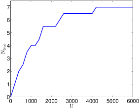
Figure 6: (Color online) Number of pair-solitons $\text{N}_{\text{Sol}}$ in each solitonic train versus HGdT potential depth $U$ in dimensionless units.

VI Summary and Conclusion

We have developed a simple quasi 1D model both analytically and numerically to calculate the statics and dynamics of the red/blue-detuned HGdT imprint upon the ${}^{87}\text{Rb}$ condensate. First of all, we showed a quantitative comparison between the Thomas-Fermi approximation and numerical solutions for the underlying 1D Gross-Pitaevskii equation for the equilibrium properties of the proposed system. Later we discussed that the HGdT potential imprint upon the condensate wave function strongly depends upon whether the effective HGdT is red- or blue-detuned. With this we found out that the HGdT imprint generates two bumps/dips at the center of the BEC density of the red/blue-detuned HGdT. Later we discussed that the red-detuned HGdT induced two bumps did not decay when we switched off the harmonic trap but the blue-detuned HGdT induced two dips decay. During the time of flight, we saw the emergence of matter-wave stripes at the top of the condensate, which arise as the BEC decomposes into a fraction at rest in the center and two moving condensates at the borders. We have used the quasi one-dimensional time-dependent GPE to analyze the creation of gray/dark pair-solitons bi-trains within the moderately/fully fragmented BEC, which is strongly depending upon the HGdT potential depth. The Hermite-Gaussian dimple trap geometry maybe more applicable to soliton interferometry rather than the Gaussian barrier adopted in Refs. J. H. V. Nguyen et al. (2014); Akram and Pelster (2015), because one can shape solitons. Additionally, we also showed that the number of pair-solitons in the system is depending on the initial HGdT potential depth $U$. During the generation of pair-solitons it was astonishing to find that the special shape of the newly generated solitons in the harmonically trapped BEC is sculptured by the external potential and the generation of gray/dark pair-solitons bi-trains is a generic phenomenon of collisions of moderately/fully fragmented BEC. With this we conclude that it maybe possible in the future to frame complex shapes of solitons in the harmonically trapped BEC by imposing a unique geometrical configuration for the external potential.

The ability of sculpting a quasi one-dimensional harmonic trapped Bose-Einstein condensate by a HGdT has many exciting prospects. For instance, it can be used to generate a truly continuous atom laser, which has many applications in atom interferometry Cronin et al. (2009); B. G. Kleine et al. (2010). To construct such an atom laser one needs a device that continuously converts a source of condensed atoms into a laser-like beam. In Sec. IV, we saw in the time-of-flight picture for the case $U>U_{\text{c}}$ that a BEC reservoir occurs at the center of the trap. By suitably tuning the HGdT depth a fraction of this fragmented condensate could be coupled out, serving as a source for an atomic beam.

VII Acknowledgment

We thank Thomas Bush for insightful comments. Furthermore, we gratefully acknowledge financial support from the German Academic Exchange Service (DAAD). This work was also supported in part by the German-Brazilian DAAD-CAPES program under the project name “Dynamics of Bose-Einstein Condensates Induced by Modulation of System Parameters” and by the German Research Foundation (DFG) via the Collaborative Research Center SFB/TR49 “Condensed Matter Systems with Variable Many-Body Interactions”.

References

- Stamper-Kurn et al. (1998) D. M. Stamper-Kurn, H.-J. Miesner, A. P. Chikkatur, S. Inouye, J. Stenger, and W. Ketterle, Phys. Rev. Lett. 81, 2194 (1998).
- Madison et al. (2000) K. W. Madison, F. Chevy, W. Wohlleben, and J. Dalibard, Phys. Rev. Lett. 84, 806 (2000).
- Madison et al. (2001) K. W. Madison, F. Chevy, V. Bretin, and J. Dalibard, Phys. Rev. Lett. 86, 4443 (2001).
- Barrett et al. (2001) M. D. Barrett, J. A. Sauer, and M. S. Chapman, Phys. Rev. Lett. 87, 010404 (2001).
- Gustavson et al. (2001) T. L. Gustavson, A. P. Chikkatur, A. E. Leanhardt, A. Görlitz, S. Gupta, D. E. Pritchard, and W. Ketterle, Phys. Rev. Lett. 88, 020401 (2001).
- Hammes et al. (2002) M. Hammes, D. Rychtarik, H.-C. Nägerl, and R. Grimm, Phys. Rev. A 66, 051401 (2002).
- Comparat et al. (2006) D. Comparat, A. Fioretti, G. Stern, E. Dimova, B. L. Tolra, and P. Pillet, Phys. Rev. A 73, 043410 (2006).
- Scherer et al. (2007) D. R. Scherer, C. N. Weiler, T. W. Neely, and B. P. Anderson, Phys. Rev. Lett. 98, 110402 (2007).
- Schulz et al. (2007) M. Schulz, H. Crepaz, F. Schmidt-Kaler, J. Eschner, and R. Blatt, J. Mod. Opt. 54, 1619 (2007).
- Tuchendler et al. (2008) C. Tuchendler, A. M. Lance, A. Browaeys, Y. R. P. Sortais, and P. Grangier, Phys. Rev. A 78, 033425 (2008).
- Jacob et al. (2011) D. Jacob, E. Mimoun, L. D. Sarlo, M. Weitz, J. Dalibard, and F. Gerbier, New J. Phys. 13, 065022 (2011).
- Garrett et al. (2011) M. C. Garrett, A. Ratnapala, E. D. van Ooijen, C. J. Vale, K. Weegink, S. K. Schnelle, O. Vainio, N. R. Heckenberg, H. Rubinsztein-Dunlop, and M. J. Davis, Phys. Rev. A 83, 013630 (2011).
- Diener et al. (2002) R. B. Diener, B. Wu, M. G. Raizen, and Q. Niu, Phys. Rev. Lett. 89, 070401 (2002).
- Proukakis et al. (2006) N. P. Proukakis, J. Schmiedmayer, and H. T. C. Stoof, Phys. Rev. A 73, 053603 (2006).
- Carpentier et al. (2008) A. Carpentier, J. Belmonte-Beitia, H. Michinel, and M. Rodas-Verde, J. Mod. Opt. 55, 2819 (2008).
- Aioi et al. (2011) T. Aioi, T. Kadokura, T. Kishimoto, and H. Saito, Phys. Rev. X 1, 021003 (2011).
- Uncu et al. (2011) H. Uncu, D. Tarhan, E. Demiralp, and O. Mustecaplioglu, Laser Physics 18, 331 (2011).
- Weitenberg et al. (2011) C. Weitenberg, S. Kuhr, K. Mølmer, and J. F. Sherson, Phys. Rev. A 84, 032322 (2011).
- Akram and Pelster (2015) J. Akram and A. Pelster, ArXiv:1508.05482 (2015).
- Raman et al. (1999) C. Raman, M. Köhl, R. Onofrio, D. S. Durfee, C. E. Kuklewicz, Z. Hadzibabic, and W. Ketterle, Phys. Rev. Lett. 83, 2502 (1999).
- Onofrio et al. (2000) R. Onofrio, C. Raman, J. M. Vogels, J. R. Abo-Shaeer, A. P. Chikkatur, and W. Ketterle, Phys. Rev. Lett. 85, 2228 (2000).
- Raman et al. (2001) C. Raman, J. R. Abo-Shaeer, J. M. Vogels, K. Xu, and W. Ketterle, Phys. Rev. Lett. 87, 210402 (2001).
- Neely et al. (2010) T. W. Neely, E. C. Samson, A. S. Bradley, M. J. Davis, and B. P. Anderson, Phys. Rev. Lett. 104, 160401 (2010).
- Saleh and Teich (2007) B. Saleh and M. Teich, Fundamentals of Photonics (Wiley, New York, 2007).
- Milonni and Eberly (2010) P. Milonni and J. Eberly, Laser Physics (Wiley, New York, 2010).
- Kozawa and Sato (2005) Y. Kozawa and S. Sato, Opt. Lett. 30, 3063 (2005).
- Flores-Pérez et al. (2006) A. Flores-Pérez, J. Hernández-Hernández, R. Jáuregui, and K. Volke-Sepúlveda, Opt. Lett. 31, 1732 (2006).
- Novitsky and Barkovsky (2006) A. V. Novitsky and L. M. Barkovsky, J. Phys. A: Math. Gen. 39, 13355 (2006).
- Mushiake et al. (1972) Y. Mushiake, K. Matsumura, and N. Nakajima, Proceedings of the IEEE 60, 1107 (1972).
- Dorn et al. (2003) R. Dorn, S. Quabis, and G. Leuchs, Phys. Rev. Lett. 91, 233901 (2003).
- Török and Munro (2004) P. Török and P. Munro, Opt. Exp. 12, 3605 (2004).
- Toussaint et al. (2005) K. C. Toussaint, S. Park, J. E. Jureller, and N. F. Scherer, Opt. Lett. 30, 2846 (2005).
- Tidwell et al. (1993) S. C. Tidwell, G. H. Kim, and W. D. Kimura, Appl. Opt. 32, 5222 (1993).
- Stalder and Schadt (1996) M. Stalder and M. Schadt, Opt. Lett. 21, 1948 (1996).
- Neil et al. (2002) M. A. A. Neil, F. Massoumian, R. Juškaitis, and T. Wilson, Opt. Lett. 27, 1929 (2002).
- Meyrath et al. (2005) T. Meyrath, F. Schreck, J. Hanssen, C. Chuu, and M. Raizen, Opt. Exp. 13, 2843 (2005).
- Smith et al. (2005) N. L. Smith, W. H. Heathcote, G. Hechenblaikner, E. Nugent, and C. J. Foot, J. Phys. B: At., Mol. Opt. Phys. 38, 223 (2005).
- Pitaevskii and Stringari (2003) L. Pitaevskii and A. Stringari, Bose-Einstein Condensation (Clarendon Press, Oxford, 2003).
- Pethick and Smith (2008) C. J. Pethick and H. Smith, Bose-Einstein Condensation in Dilute Gases, 2nd ed. (Cambridge University Press, Cambridge, 2008).
- Kevrekidis et al. (2008) P. G. Kevrekidis, D. Frantzeskakis, and R. Carretero-González, Emergent Nonlinear Phenomena in Bose-Einstein Condensates (Springer, Berlin, 2008).
- Olshanii (1998) M. Olshanii, Phys. Rev. Lett. 81, 938 (1998).
- Petrov et al. (2000) D. S. Petrov, G. V. Shlyapnikov, and J. T. M. Walraven, Phys. Rev. Lett. 85, 3745 (2000).
- Bergeman et al. (2003) T. Bergeman, M. G. Moore, and M. Olshanii, Phys. Rev. Lett. 91, 163201 (2003).
- Pérez-García et al. (1998) V. M. Pérez-García, H. Michinel, and H. Herrero, Phys. Rev. A 57, 3837 (1998).
- Jackson et al. (1998) A. D. Jackson, G. M. Kavoulakis, and C. J. Pethick, Phys. Rev. A 58, 2417 (1998).
- Carr et al. (2000a) L. D. Carr, M. A. Leung, and W. P. Reinhardt, J. Phys. B: At., Mol. Opt. Phys. 33, 3983 (2000a).
- Carr et al. (2000b) L. D. Carr, C. W. Clark, and W. P. Reinhardt, Phys. Rev. A 62, 063611 (2000b).
- Adhikari (2006) S. K. Adhikari, Las. Phys. Lett. 3, 553 (2006).
- Strecker et al. (2003) K. E. Strecker, G. B. Partridge, A. G. Truscott, and R. G. Hulet, New J. Phys. 5, 73 (2003).
- Abdullaev et al. (2004) F. K. Abdullaev, A. Gammal, and L. Tomio, J. Phys. B: At. Mol. Opt. Phys. 37, 635 (2004).
- Herring et al. (2005) G. Herring, P. Kevrekidis, R. Carretero-González, B. Malomed, D. Frantzeskakis, and A. Bishop, Phys. Lett. A 345, 144 (2005).
- C. Becker et al. (2008) C. Becker, S. Stellmer, P. Soltan-Panahi, S. Dorscher, M. Baumert, E.M. Richter, J. Kronjager, K. Bongs, and K. Sengstock, Nature Phys. 4, 496 (2008).
- Denschlag et al. (2000) J. Denschlag, J. E. Simsarian, D. L. Feder, C. W. Clark, L. A. Collins, J. Cubizolles, L. Deng, E. W. Hagley, K. Helmerson, W. P. Reinhardt, S. L. Rolston, B. I. Schneider, and W. D. Phillips, Science 287, 97 (2000).
- Huang et al. (2002) G. Huang, J. Szeftel, and S. Zhu, Phys. Rev. A 65, 053605 (2002).
- Radouani (2004) A. Radouani, Phys. Rev. A 70, 013602 (2004).
- Yan et al. (2012) D. Yan, J. J. Chang, C. Hamner, M. Hoefer, P. G. Kevrekidis, P. Engels, V. Achilleos, D. J. Frantzeskakis, and J. Cuevas, J. Phys. B: At. Mol. Opt. Phys. 45, 115301 (2012).
- Hans et al. (2015) I. Hans, J. Stockhofe, and P. Schmelcher, Phys. Rev. A 92, 013627 (2015).
- Chang et al. (2008) J. J. Chang, P. Engels, and M. A. Hoefer, Phys. Rev. Lett. 101, 170404 (2008).
- Meppelink et al. (2009) R. Meppelink, S. B. Koller, J. M. Vogels, P. van der Straten, E. D. van Ooijen, N. R. Heckenberg, H. Rubinsztein-Dunlop, S. A. Haine, and M. J. Davis, Phys. Rev. A 80, 043606 (2009).
- Allen and Eberly (1987) L. Allen and J. H. Eberly, Optical Resonance and Two-Level Atoms (Wiley, New York, 1987).
- Scully and Zubairy (1997) M. O. Scully and M. S. Zubairy, Quantum Optics, 1st ed. (Cambridge University Press, 1997).
- Xu et al. (2010) P. Xu, X. He, J. Wang, and M. Zhan, Opt. Lett. 35, 2164 (2010).
- Kamchatnov (2004) A. Kamchatnov, J. Exp. Theor. Phys. 98, 908 (2004).
- Bongs and Sengstock (2004) K. Bongs and K. Sengstock, Rep. Prog. Phys. 67, 907 (2004).
- Yin (2006) J. Yin, Phys. Rep. 430, 1 (2006).
- Vudragović et al. (2012) D. Vudragović, I. Vidanović, A. Balaž, P. Muruganandam, and S. K. Adhikari, Comp. Phys. Commun. 183, 2021 (2012).
- Kumar et al. (2015) R. K. Kumar, L. E. Young-S., D. Vudragović, A. Balaž, P. Muruganandam, and S. Adhikari, Comput. Phys. Commun. 195, 117 (2015).
- Lončar et al. (2016) V. Lončar, A. Balaž, A. Bogojević, S. Škrbić, P. Muruganandam, and S. K. Adhikari, Comput. Phys. Commun. 200, 406 (2016).
- Satarić et al. (2016) B. Satarić, V. Slavnić, A. Belić, A. Balaž, P. Muruganandam, and S. K. Adhikari, Comput. Phys. Commun. 200, 411 (2016).
- Busch and Anglin (2001) T. Busch and J. R. Anglin, Phys. Rev. Lett. 87, 010401 (2001).
- Scott et al. (1998) T. F. Scott, R. J. Ballagh, and K. Burnett, J. Phys. B: At., Mol. Opt. Phys. 31, L329 (1998).
- Weller et al. (2008) A. Weller, J. P. Ronzheimer, C. Gross, J. Esteve, M. K. Oberthaler, D. J. Frantzeskakis, G. Theocharis, and P. G. Kevrekidis, Phys. Rev. Lett. 101, 130401 (2008).
- Shomroni et al. (2009) I. Shomroni, E. Lahoud, S. Levy, and J. Steinhauer, Nature Phys. 5, 193 (2009).
- J. H. V. Nguyen et al. (2014) J. H. V. Nguyen, P. Dyke, D. Luo, B. A. Malomed, and R. G. Hulet, Nature Phys. 10, 918 (2014).
- Cronin et al. (2009) A. D. Cronin, J. Schmiedmayer, and D. E. Pritchard, Rev. Mod. Phys. 81, 1051 (2009).
- B. G. Kleine et al. (2010) B. G. Kleine, J. Will, W. Ertmer, C. Klempt, and J. Arlt, Appl. Phys. B 100, 117 (2010).