Parareal convergence for 2D unsteady flow around a cylinder

Abstract

In this technical report we study the convergence of Parareal for 2D incompressible flow around a cylinder for different viscosities. Two methods are used as fine integrator: backward Euler and a fractional step method. It is found that Parareal converges better for the implicit Euler, likely because it under-resolves the fine-scale dynamics as a result of numerical diffusion.

1 Introduction

The potential of parallel-in-time integration methods to increase the degree of concurrency in the numerical solution of time-dependent partial differential equations has been widely acknowledged, e.g. in the report Applied Mathematics Research for Exascale Computing by Dongarra et al. (2014). A variety of different methods exists, see e.g. the review by Gander (2015), and principle efficiency of parallel-in-time integration in large- and extreme-scale parallel computations has been demonstrated, e.g. in  Speck et al. (2012); Ruprecht et al. (2013), and Gander and Neumueller (2014).

Many problems in computational fluid dynamics require massive computational capacities and suffer from long solution times. Exploring the potential of parallel-in-time methods to speed up such simulations can therefore be a beneficial endeavour. The performance of the parallel-in-time integration method Parareal, introduced by Lions et al. (2001), when applied to the Navier-Stokes equations has been a topic of research since shortly after its introduction. First studies have been conducted by Trindade and Pereira (2004, 2006), including reports of speedup for an MPI implementation; laminar flow around a cylinder is used as benchmark problem and it is shown that Parareal can correctly reproduce the Nusselt number. Fischer et al. (2005) investigate Parareal for spatial discretisations based on finite and spectral element methods, and discuss using fewer spatial degrees-of-freedom for the coarse integrator. The performance of Parareal for simulations of non-Newtonian fluids has been investigated by Celledoni and Kvamsdal (2009). Finally, parallel scaling of Parareal for 3D unsteady flow is investigated by Croce et al. (2014) on up to $2048$ cores.

Based on predictions from linear stability analysis by Gander and Vandewalle (2007), it has been shown by Steiner et al. (2015)) that convergence of Parareal deteriorates as the Reynolds number increases. However, the studies only analysed a rather simple driven cavity problem, which eventually approaches a steady-state and thus may underestimate the problem because of weak transient dynamics towards the end of the simulation. In this report, we continue this investigation for a different, more complex benchmark involving unsteady flow around a cylinder. It was introduced by Schäfer et al. (1996) as the case $2$D-$3$ and further analyzed by e.g. John (2004). Eventually, the here presented benchmarks will be extended to a comprehensive exploration of Parareal’s performance for 3D flow, including a study of the influence of spatial resolution.

2 Parareal and model problem

2.1 Parareal

Parareal parallelises the solution of initial value problems

$$u_{t}=f(t,u(t)),\quad u(0)=u_{0},\quad t\in[0,T],$$ (1)

by decomposing the time domain $[0,T]$ into time slices $[t_{j-1},t_{j}]$, $j=1,\ldots,N_{\text{pr}}$ with $N_{\text{pr}}$ equal to the number of processing units. It then iterates between two time integration methods: a coarse integrator $\mathcal{C}$ used to serially propagate corrections, which has to be computationally cheap, and an accurate integrator $\mathcal{F}$ run in parallel. The Parareal iteration reads

$$u^{k+1}_{j+1}=\mathcal{C}(u^{k+1}_{j})+\mathcal{F}(u^{k}_{j})-\mathcal{C}(u^{k}_{j}),\quad j=1,\ldots,N_{\text{pr}},$$ (2)

with $k$ being the iteration index and $u_{j}\approx u(t_{j})$. Note how the computationally expensive computation of the fine method can be done concurrently for all time slices. A detailed presentation including a theoretical model for projected speedup is given e.g. by Minion (2010).

2.2 Model problem

As model problem, we consider the Navier-Stokes equations

$$(\partial_{t}+\boldsymbol{U}\boldsymbol{\nabla})\boldsymbol{U}=-\frac{\boldsymbol{\nabla}p}{\varrho}+\nu\boldsymbol{\nabla}^{2}\boldsymbol{U}$$ (3)

for an incompressible fluid, i.e. for a fluid with $\boldsymbol{\nabla}\boldsymbol{U}=0$, at density $\varrho\mathrel{\mathop{:}}=1\ (\text{kg}/\text{m}^{2})$. We focus on the benchmark problem defined in Schäfer et al. (1996) as $2$D-$3$, which is for unsteady flow around a cylinder in two dimensions, i.e. in $2$D (see also John (2004)). We make use of the definitions

$$\boldsymbol{\nabla}\mathrel{\mathop{:}}=(\partial_{x},\partial_{y})^{\text{T}},\qquad\boldsymbol{U}\mathrel{\mathop{:}}=\boldsymbol{U}(t,x,y),\qquad\boldsymbol{U}\mathrel{\mathop{:}}=(u,v)^{\text{T}}.$$ (4)

The Reynolds number for a cylinder with diameter $d$ (the reference length) located inside a square cuboid with longest edge along the $x$-coordinate is

$$R_{d}\mathrel{\mathop{:}}=\bar{u}_{\text{in}}\frac{d}{\nu},$$ (5)

where the reference velocity $\bar{u}_{\text{in}}$ is chosen to be the mean velocity of inflow in $x$-direction and $\nu$ the kinematic viscosity. Notice that $R_{d}$ can be time dependent, as is the case for the problem considered here.

In the $2$D case the mean velocity is

$$\bar{u}(t)\mathrel{\mathop{:}}=\int_{0}^{h}\frac{u(t,0,y)}{h}\ \text{\text{d}}y=\frac{2}{3}u\left(t,0,\frac{h}{2}\right),\qquad\bar{v}(t)\mathrel{\mathop{:}}=0,$$ (6)

where $h\mathrel{\mathop{:}}=0.41\ (\text{m})$. In the $2$D-$3$ case we have the inflow velocity

$$u_{\text{in}}(t,0,y)\mathrel{\mathop{:}}=4u^{\text{x}}_{\text{in}}\sin\left(\frac{\pi}{8}t\right)\frac{y(h-y)}{h^{2}},\qquad v_{\text{in}}(t,0,y)\mathrel{\mathop{:}}=0,$$ (7)

for which Equation (6) is valid. We choose $u^{\text{x}}_{\text{in}}\mathrel{\mathop{:}}=3/2\ (\text{m}/\text{s})$ so that

$$R_{d}(t)=\sin\left(\frac{\pi}{8}t\right)\frac{d}{\nu}\in\left[0,\frac{d}{\nu}\right].$$ (8)

Thus, setting $d\mathrel{\mathop{:}}=0.1\ (\text{m})$, it follows for $\nu\in\{0.1,0.01,0.001\}\ (\text{m}/\text{s})$ that

$$R^{\text{x}}_{d}\in\{1,10,100\}$$ (9)

defines the maximum-over-time Reynolds number for the chosen $\nu$.

In this report, the primary goal is to outline the performance of Parareal for the $2$D-$3$ benchmark problem for the three mentioned viscosities, i.e. ranges of Reynolds numbers.

2.3 Implementation details

The governing equations were implemented using Q2-Q1 finite elements in the UG4 software toolbox (see Vogel et al. (2013); Vogel (2014)). For the parallelisation in time via Parareal, we used the library Lib4PrM, which was first applied in Kreienbuehl et al. (2015).

3 Results

Instead of measuring convergence of Parareal by comparing the discretisation error with the defect as discussed e.g. by Arteaga et al. (2015), we focus here on how well Parareal reproduces important characteristic numbers of the dynamics, namely the drag coefficient $C_{\text{dr}}$, the lift coefficient $C_{\text{li}}$ and the pressure difference $\Delta_{p}$ between the front and end point of the cylinder over time. These parameters are respectively defined as follows:

$$C_{\text{dr}}\mathrel{\mathop{:}}=\frac{2F_{\text{dr}}}{\varrho\bar{u}^{2}_{\text{in}}d},\qquad C_{\text{li}}\mathrel{\mathop{:}}=\frac{2F_{\text{li}}}{\varrho\bar{u}^{2}_{\text{in}}d},\qquad\Delta_{p}\mathrel{\mathop{:}}=p_{\text{fr}}-p_{\text{en}},$$ (10)

where $F_{\text{dr}}$ is the drag force and $F_{\text{li}}$ the lift force, and $p_{\text{fr}}$ together with $p_{\text{en}}$ define the pressure at the front and end of the cylinder. Again, we assume here that the density is $1\ (\text{kg}/\text{m}^{2})$ and set $t\in[0,8]\ (\text{s})$ as time domain.

For $\nu=0.001\ (\text{m}/\text{s})$, Schäfer et al. (1996) report on a maximum-over-time drag coefficient of $C^{\text{ma}}_{\text{dr}}\approx 2.9500\pm 0.0200$, a maximum-over-time lift coefficient of $C^{\text{ma}}_{\text{li}}\approx 0.4800\pm 0.0100$, and a final pressure difference at $t=8\ (\text{s})$ of $\Delta^{\text{fi}}_{p}\approx-0.1100\pm 0.0050\ (\text{kg}/\text{s}^{2})$.

3.1 Numerical setup

We use $N_{\text{pr}}\in\{2,4,8,16\}$ processors without parallelization in space and with $13,\!212$ spatial degrees-of-freedom for both the fine and coarse level. For each $\nu$, we consider the following two Parareal solvers “S” comprised of a coarse $\text{M}_{\text{co}}$ and fine $\text{M}_{\text{fi}}$ serial time integration method as well as number of time steps $N_{\text{co}}$ and $N_{\text{fi}}$:

$$(\text{M}_{\text{co}},N_{\text{co}})\times(\text{M}_{\text{fi}},N_{\text{fi}}) =(\text{IE},16)\times(\text{IE},32), \text{S}_{1}$$ ()

$$(\text{M}_{\text{co}},N_{\text{co}})\times(\text{M}_{\text{fi}},N_{\text{fi}}) =(\text{IE},16)\times(\text{FS},32), \text{S}_{2}$$ ()

where “IE” stands for implicit Euler (first-order) and “FS” for fractional step (second-order). Errors in the three physical quantities discussed above are measured by

$$E_{\text{ph}}\mathrel{\mathop{:}}=\frac{\|u^{\text{pa}}_{\text{ph}}-u^{\text{fi}}_{\text{ph}}\|_{\text{ti}}}{\|u^{\text{fi}}_{\text{ph}}\|_{\text{ti}}},$$ (11)

where the parameter “ph” is in $\{$dr,li,$p\}$ for drag and lift coefficient or pressure difference. We use the $l_{2}$-norm over the solutions at the end of all time-slices

$$\|u\|^{2}_{\text{ti}}\mathrel{\mathop{:}}=\frac{8}{N_{\text{pr}}}\sum_{n=1}^{N_{\text{pr}}}|u(t^{n})|^{2}$$ (12)

weighted by the time slice length $8/N_{\text{pr}}$.

3.2 Problem dynamics

Figure 1 shows the flow field at $t=5.25\ (\text{s})$ for the three different viscosities. As viscosity decreases, the maximum Reynolds number increases and the flow becomes more turbulent. While for $\nu=0.1\ (\text{m}/\text{s})$ and $\nu=0.01\ (\text{m}/\text{s})$ the flow is essentially laminar, smaller vortices start to form behind the cylinder for $\nu=0.001\ (\text{m}/\text{s})$.

Figure 1: Flow field at $t=5.25\ (\text{s})$ for three different viscosities: $\nu=0.1\ (\text{m}/\text{s})$ at the top, $\nu=0.01\ (\text{m}/\text{s})$ in the middle, and $\nu=0.001\ (\text{m}/\text{s})$ at the bottom.

The resulting evolution over time of the three characteristic numbers for $\nu=0.1\ (\text{m}/\text{s})$ using serial time integration is shown in Figure 2. Both fine integrators $S_{1}$ and $S_{2}$ produce essentially identical profiles and their profiles closely match the one generated by the corresponding reference simulation (not shown).

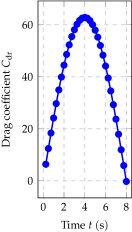
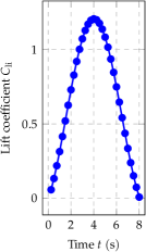
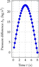
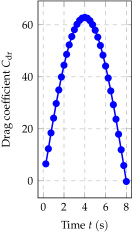
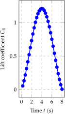
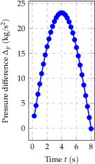
Figure 2: Drag and lift coefficient, and pressure difference for $\nu=0.1\ (\text{m}/\text{s})$ for $S_{1}$ (top) and $S_{2}$ (bottom). The curves match the values from the reference simulation (not shown).

Figure 3 shows the same profiles for the simulation with $\nu=0.01\ (\text{m}/\text{s})$. Again, both $S_{1}$ and $S_{2}$ produce profiles that match and agree with the results from the corresponding reference (not shown).

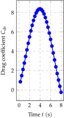
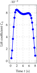
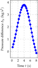
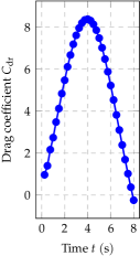
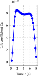
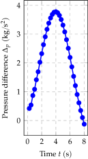
Figure 3: Drag and lift coefficient, and pressure difference for $\nu=0.01\ (\text{m}/\text{s})$ for reference (top), $S_{1}$ (middle) and $S_{2}$ (bottom).

Lastly, Figure 4 shows three profiles for $\nu=0.001\ (\text{m}/\text{s})$, one for the reference simulation, one for $S_{1}$ and one for $S_{2}$. While the drag coefficient and pressure difference agree across all three configurations, $S_{1}$ produces a lift coefficient profile that is distinctly different from the corresponding reference and $S_{2}$. The relatively high numerical diffusion of $S_{1}$ in combination with a rather low spatial resolution probably prevents $S_{1}$ from correctly capturing the more turbulent dynamics in this case. In contrast, although $S_{2}$ fails to fully reproduce the frequency of oscillations, it still achieves a qualitatively correct representation of the dynamics of the corresponding reference simulation.

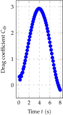
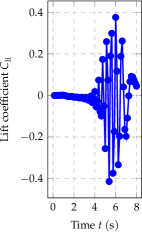
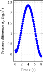
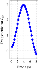
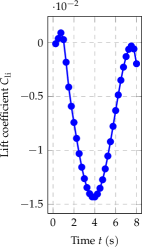
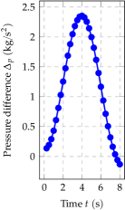
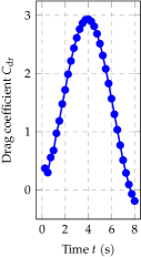
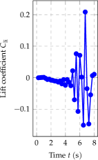
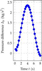
Figure 4: Drag and lift coefficient, and pressure difference for $\nu=0.001\ (\text{m}/\text{s})$ for reference (top), $S_{1}$ (middle) and $S_{2}$ (bottom).

3.3 Convergence of Parareal

Here, we analyse how accurately Parareal reproduces the three characteristic values studied above. Figure 5 shows the defect or error according to Equation (11) in the characteristic values accumulated over all time slices versus the number of iterations. Here, defect refers to the difference between the solution computed by Parareal and the solution computed by running the fine integrator serially. For $S_{1}$, the error for all three quantities, i.e. drag coefficient, lift coefficient and pressure difference, quickly goes to zero, that is Parareal rapidly produces values identical to ones obtained from the serial simulation. As the number of time slices is increased, convergence becomes slower but the increase is not drastic: for $N_{\text{pr}}=16$ after seven iterations all three characteristic values have converged up to round-off error. In a production run, where the main goal is to push the defect from Parareal below the discretisation error (see the discussion in Arteaga et al. (2015)), significantly fewer iterations will likely suffice.

Decreasing viscosity and thus increasing the Reynolds number range does negatively affect convergence. For $\nu=0.001\ (\text{m}/\text{s})$, the simulation with $N_{\text{pr}}=16$ time slices already requires $13$ iterations to converge up to round-off error. Depending on the desired accuracy, speedup is still possible here but parallel efficiency will likely be lower than in the more laminar case. Since $S_{1}$ fails to resolve the full dynamics of the problem, its convergence behaviour is probably not representative of the actual physical dynamics.

This is supported by the fact that for $S_{2}$ and $\nu=0.001\ (\text{m}/\text{s})$, Parareal essentially no longer converges. Since $S_{2}$ does resolve the turbulent dynamics at least partially, in contrast to $S_{1}$, this suggests that the good convergence of Parareal for $S_{1}$ and $\nu=0.001\ (\text{m}/\text{s})$ is an artefact produced by excessive numerical diffusion. The dynamics of the numerical solution are more laminar than they should be, leading to an unrealistic convergence behaviour of Parareeal. Supposedly, when using $S_{1}$ on a significantly finer spatial and temporal mesh, a similar deterioration of convergence would be observed, as the numerical solution better resolves the turbulent features of the flow.

Interestingly, this difference between $S_{1}$ and $S_{2}$ can already be seen for $\nu=0.1\ (\text{m}/\text{s})$, where the physical dynamics are still quite laminar as well. Although Parareal for $S_{2}$ does converge, particularly for larger numbers of time slices, its rate of convergence is lower than for $S_{1}$. The benefit of using an integrator with damping properties as coarse integrator has been pointed out before by Bal (2005) but apparently numerical diffusion from the fine method does help Parareal convergence, too. Since here the fine method realistically represents the flow features, using a diffusive integrator as fine method in Parareal when simulating turbulent flow could be an easy way to obtain decent convergence.

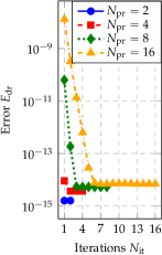
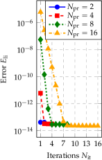
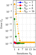
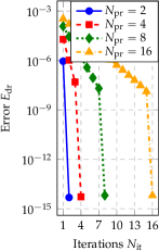
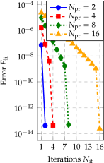
Figure 5: Fine solver convergence errors for drag and lift coefficient, and pressure difference for $\nu=0.1\ (\text{m}/\text{s})$ and $S_{1}$ (top) and $S_{2}$ (bottom).

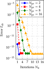
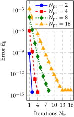
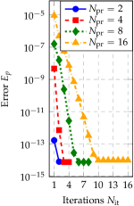
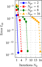
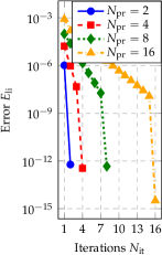
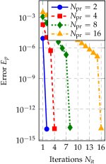
Figure 6: Fine solver convergence errors for drag and lift coefficient, and pressure difference for $\nu=0.01\ (\text{m}/\text{s})$ for $S_{1}$ (top) and $S_{2}$ (bottom).

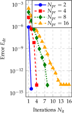
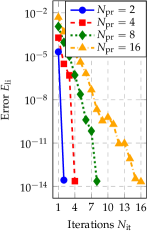
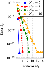
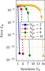
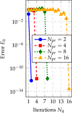
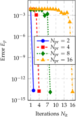
Figure 7: Fine solver convergence errors for drag and lift coefficient, and pressure difference for $\nu=0.001\ (\text{m}/\text{s})$ for $S_{1}$ (top) and $S_{2}$ (bottom).

4 Conclusions

This report extends the investigation by Steiner et al. (2015) about how a decreasing viscosity in the Navier-Stokes equations affects the convergence behaviour of the Parareal parallel-in-time method. An unsteady 2D flow around a cylinder is used as a benchmark. Two different configurations are tested, one using an implicit Euler as coarse and fine method, the other an implicit Euler as coarse but a second-order fractional step integrator as fine method. For larger viscosities, both base methods correctly reproduce the evolution of characteristic quantities like drag and lift coefficient and pressure difference. However, the numerical diffusion from the backward Euler method as fine integrator leads to significantly better convergence of Parareal.

As viscosity decreases, convergence of Parareal becomes slower similarly to the results in Steiner et al. (2015). However, while for the fractional step method Parareal stalls completely, the backward Euler retains reasonable convergence even for small viscosities. A comparison of the profiles for characteristic numbers with a reference solution suggests that the good convergence for the backward Euler is likely artificial. The fine integrator alone captures the relatively smooth profiles of the drag coefficient and pressure difference quite well. However, the high frequency oscillations in the lift coefficient, which are clearly seen in serial runs using the fractional step integrator, are not present when using backward Euler. Most likely, the rather high numerical diffusion leads to an artificially laminar flow, so that the good convergence of Parareal is not representative of the used viscosity parameter. Clearly, when assessing Parareal’s convergence for flow problems, care must be taken to ensure that the fine base method correctly resolves the important features of the flow. Intrinsic convergence of Parareal alone is not a reliable indicator.

There are several works proposing strategies to stabilise Parareal for advection-dominated problems, e.g. by Farhat et al. (2006), Gander and Petcu (2008), Ruprecht and Krause (2012) or Chen et al. (2014). An interesting continuation of the work presented here would be to analyse whether these strategies improve convergence of Parareal for turbulent flows.

References

- Arteaga et al. [2015] A. Arteaga, Daniel Ruprecht, and Rolf Krause. A stencil-based implementation of Parareal in the C++ domain specific embedded language STELLA. Applied Mathematics and Computation, 2015. URL http://dx.doi.org/10.1016/j.amc.2014.12.055.
- Bal [2005] Guillaume Bal. On the convergence and the stability of the parareal algorithm to solve partial differential equations. In Ralf Kornhuber and et al., editors, Domain Decomposition Methods in Science and Engineering, volume 40 of Lecture Notes in Computational Science and Engineering, pages 426–432, Berlin, 2005. Springer. URL http://dx.doi.org/10.1007/3-540-26825-1_43.
- Celledoni and Kvamsdal [2009] E. Celledoni and T. Kvamsdal. Parallelization in time for thermo-viscoplastic problems in extrusion of aluminium. International Journal for Numerical Methods in Engineering, 79(5):576–598, 2009. URL http://dx.doi.org/10.1002/nme.2585.
- Chen et al. [2014] Feng Chen, Jan S. Hesthaven, and Xueyu Zhu. On the Use of Reduced Basis Methods to Accelerate and Stabilize the Parareal Method. In Alfio Quarteroni and Gianluigi Rozza, editors, Reduced Order Methods for Modeling and Computational Reduction, volume 9 of MS&A - Modeling, Simulation and Applications, pages 187–214. Springer International Publishing, 2014. URL http://dx.doi.org/10.1007/978-3-319-02090-7_7.
- Croce et al. [2014] Roberto Croce, Daniel Ruprecht, and Rolf Krause. Parallel-in-Space-and-Time Simulation of the Three-Dimensional, Unsteady Navier-Stokes Equations for Incompressible Flow. In Hans Georg Bock, Xuan Phu Hoang, Rolf Rannacher, and Johannes P. Schlöder, editors, Modeling, Simulation and Optimization of Complex Processes – HPSC 2012, pages 13–23. Springer International Publishing, 2014. URL http://dx.doi.org/10.1007/978-3-319-09063-4_2.
- Dongarra et al. [2014] Jack Dongarra et al. Applied Mathematics Research for Exascale Computing. Technical Report LLNL-TR-651000, Lawrence Livermore National Laboratory, 2014. URL http://science.energy.gov/~/media/ascr/pdf/research/am/docs/EMWGreport.pdf.
- Farhat et al. [2006] Charbel Farhat, Julien Cortial, C. Dastillung, and H. Bavestrello. Time-parallel implicit integrators for the near-real-time prediction of linear structural dynamic responses. International Journal for Numerical Methods in Engineering, 67:697–724, 2006. URL http://dx.doi.org/10.1002/nme.1653.
- Fischer et al. [2005] P. F. Fischer, F. Hecht, and Yvon Maday. A parareal in time semi-implicit approximation of the Navier-Stokes equations. In Ralf Kornhuber and et al., editors, Domain Decomposition Methods in Science and Engineering, volume 40 of Lecture Notes in Computational Science and Engineering, pages 433–440, Berlin, 2005. Springer. URL http://dx.doi.org/10.1007/3-540-26825-1_44.
- Gander [2015] Martin J. Gander. 50 years of Time Parallel Time Integration. In Multiple Shooting and Time Domain Decomposition. Springer, 2015. URL {http://www.unige.ch/%7Egander/Preprints/50YearsTimeParallel.pdf}.
- Gander and Neumueller [2014] Martin J. Gander and M. Neumueller. Analysis of a Time Multigrid Algorithm for DG-Discretizations in Time. 2014. URL http://arxiv.org/abs/1409.5254.
- Gander and Petcu [2008] Martin J. Gander and M. Petcu. Analysis of a Krylov Subspace Enhanced Parareal Algorithm for Linear Problem. ESAIM: Proc., 25:114–129, 2008. URL http://dx.doi.org/10.1051/proc:082508.
- Gander and Vandewalle [2007] Martin J. Gander and Stefan Vandewalle. On the Superlinear and Linear Convergence of the Parareal Algorithm. In Olof B. Widlund and David E. Keyes, editors, Domain Decomposition Methods in Science and Engineering, volume 55 of Lecture Notes in Computational Science and Engineering, pages 291–298. Springer Berlin Heidelberg, 2007. URL http://dx.doi.org/10.1007/978-3-540-34469-8_34.
- John [2004] Volker John. Reference values for drag and lift of a two-dimensional time-dependent flow around a cylinder. International Journal for Numerical Methods in Fluids, 44(7):777–788, Mar 2004. doi: 10.1002/fld.679.
- Kreienbuehl et al. [2015] Andreas Kreienbuehl, Arne Naegel, Daniel Ruprecht, Robert Speck, Gabriel Wittum, and Rolf Krause. Numerical simulation of skin transport using Parareal. Computing and Visualization in Science, Aug 2015. doi: 10.1007/s00791-015-0246-y. URL http://arxiv.org/abs/1502.03645.
- Lions et al. [2001] J.-L. Lions, Yvon Maday, and Gabriel Turinici. A ”parareal” in time discretization of PDE’s. Comptes Rendus de l’Académie des Sciences - Series I - Mathematics, 332:661–668, 2001. URL http://dx.doi.org/10.1016/S0764-4442(00)01793-6.
- Minion [2010] Michael L. Minion. A Hybrid Parareal Spectral Deferred Corrections Method. Communications in Applied Mathematics and Computational Science, 5(2):265–301, 2010. URL http://dx.doi.org/10.2140/camcos.2010.5.265.
- Ruprecht and Krause [2012] Daniel Ruprecht and Rolf Krause. Explicit parallel-in-time integration of a linear acoustic-advection system. Computers & Fluids, 59(0):72–83, 2012. URL http://dx.doi.org/10.1016/j.compfluid.2012.02.015.
- Ruprecht et al. [2013] Daniel Ruprecht, Robert Speck, Matthew Emmett, Matthias Bolten, and Rolf Krause. Poster: Extreme-scale space-time parallelism. In Proceedings of the 2013 Conference on High Performance Computing Networking, Storage and Analysis Companion, SC ’13 Companion, 2013. URL http://sc13.supercomputing.org/sites/default/files/PostersArchive/tech_posters/post148s2-file3.pdf.
- Schäfer et al. [1996] Michael Schäfer, Stefan Turek, Franz Durst, Egon Krause, and Rolf Rannacher. Benchmark Computations of Laminar Flow Around a Cylinder. In Ernst Heinrich Hirschel, editor, Flow Simulation with High-Performance Computers II, volume 48 of Notes on Numerical Fluid Mechanics (NNFM), pages 547–566. Vieweg+Teubner Verlag, 1996. ISBN (13) 9783322898517. doi: 10.1007/978-3-322-89849-4“˙39.
- Speck et al. [2012] Robert Speck, Daniel Ruprecht, Rolf Krause, Matthew Emmett, Michael L. Minion, Mathias Winkel, and Paul Gibbon. A massively space-time parallel N-body solver. In Proceedings of the International Conference on High Performance Computing, Networking, Storage and Analysis, SC ’12, pages 92:1–92:11, Los Alamitos, CA, USA, 2012. IEEE Computer Society Press. URL http://dx.doi.org/10.1109/SC.2012.6.
- Steiner et al. [2015] J. Steiner, Daniel Ruprecht, Robert Speck, and Rolf Krause. Convergence of Parareal for the Navier-Stokes equations depending on the Reynolds number. In Assyr Abdulle, Simone Deparis, Daniel Kressner, Fabio Nobile, and Marco Picasso, editors, Numerical Mathematics and Advanced Applications - ENUMATH 2013, volume 103 of Lecture Notes in Computational Science and Engineering, pages 195–202. Springer International Publishing, 2015. URL http://dx.doi.org/10.1007/978-3-319-10705-9_19.
- Trindade and Pereira [2004] J. M. F. Trindade and J. C. F. Pereira. Parallel-in-time simulation of the unsteady Navier-Stokes equations for incompressible flow. International Journal for Numerical Methods in Fluids, 45(10):1123–1136, 2004. URL http://dx.doi.org/10.1002/fld.732.
- Trindade and Pereira [2006] J. M. F. Trindade and J. C. F. Pereira. Parallel-in-Time Simulation of Two-Dimensional, Unsteady, Incompressible Laminar Flows. Numerical Heat Transfer, Part B: Fundamentals, 50(1):25–40, 2006. URL http://dx.doi.org/10.1080/10407790500459379.
- Vogel [2014] Andreas Vogel. Flexible und kombinierbare Implementierung von Finite-Volumen-Verfahren höherer Ordnung mit Anwendungen für die Konvektions-Diffusions-, Navier-Stokes- und Nernst-Planck-Gleichungen sowie dichtegetriebene Grundwasserströmung in porösen Medien. PhD thesis, Johann Wolfgang Goethe-Universität Frankfurt, 2014.
- Vogel et al. [2013] Andreas Vogel, Sebastian Reiter, Martin Rupp, Arne Nägel, and Gabriel Wittum. UG 4: A novel flexible software system for simulating PDE based models on high performance computers. Computing and Visualization in Science, 16(4):165–179, Aug 2013. ISSN 1433-0369. doi: 10.1007/s00791-014-0232-9. URL http://dx.doi.org/10.1007/s00791-014-0232-9.