Neuron detection in stack images: a persistent homology interpretation

Abstract

Automation and reliability are the two main requirements when computers are applied in Life Sciences. In this paper we report on an application to neuron recognition, an important step in our long-term project of providing software systems to the study of neural morphology and functionality from biomedical images. Our algorithms have been implemented in an ImageJ plugin called NeuronPersistentJ, which has been validated experimentally. The soundness and reliability of our approach are based on the interpretation of our processing methods with respect to persistent homology, a well-known tool in computational mathematics.

Keywords: Neuron tracing; Dendrite recognition; Persistent Homology; Algebraic Topology.

1 Introduction

The pioneer works of Ramón y Cajal suggested that neuronal morphology and physiology were intrinsically correlated. The specificity of connections and information flux, as Cajal proposed, were closely dependent of neuronal structure [3].

Neuronal reconstruction and recognition were, since Cajal’s work, hindered by a similar problem: the discerning of a single neuron over hundreds of millions. Several staining techniques are employed to identify a single neuron [22]; for instance, Golgi staining, iontophoretic intracellular injection [10, 1] and Diolostic gun [13]. The use of optical and confocal microscopy and digital reconstruction of neuronal morphology has become a powerful technique for investigating the nervous system structure, providing us with a large scale collection of images.

On the other hand, dendritic neuronal trees and axonal growing are involved in neuronal computation and brain functions. Dendritic growing and axonal pathfinding are modified during brain development [15, 26] neuronal plasticity process [12] and neural disorders such autism [4] or degenerative diseases such Alzheimer; for instance, in this neurodegenerative process brains are characterized by the presence of numerous atrophic neurons near the amyloidal plaques [27, 11]. Therefore, visualization and analysis of neuronal morphology and structure is of a critical importance to elucidate physiological changes.

The majority of reconstruction available software are manual or semiautomatic (see [19]), in which axonal and dendritic process are drawing by hand and consequently are not suitable for the analysis of large arrays of data sets. Subsequently the traces would transform into a geometrical format suitable for quantitative analysis and computational modeling. Algorithmic automation of neuronal tracing promises to increase the speed, accuracy, and reproducibility of morphological reconstructions. In this way, large scale analysis is feasible and would allow a high throughput strategy for the study of nervous system morphology in pharmacology or degenerative diseases [8]. The properties of optical microscopes images make it difficult to identify and automatically trace dendrites accurately, the presence of noise and biological contaminations, i.e. dendritic segments from neighbors neurons make difficult the digital encoding and reconstruction of a single neuronal structure.

To solve these problems, here, we employ geometric persistence models to extract the dendrites and neuronal morphology from a series of inmunohistochemical images. The application developed is based on the idea that the neuron that we want to study persists in all the levels of the z-stack. The method presented in this paper is not just theoretical but also has been implemented as a new plugin, called NeuronPersistentJ [17], for the systems ImageJ [23] and Fiji [25].

The rest of this paper is organized as follows. The following section is devoted to describe the cell cultures and image acquisition methods. The procedure that we have developed for tracking neuronal morphology and its interpretation in terms of persistent homology is presented in Section 3. The experimental results obtained with our software are discussed in Section 4. The paper ends with a discussion section and the bibliography.

2 Methods

2.1 Cell cultures

Primary cultures of hippocampal neurons were prepared from postnatal (P0-P1) rat pups as described previously in [2, 20, 7]. Briefly, glass coverslips ($12$ mm diameter) were coated with poly-L-lysine ($100$ $\mu$g/ml) and laminin ($4$ $\mu$g/ml). In brief, hippocampal neurons were seeded at 15000/cm² in culture medium consisting on Neurobasal medium (Invitrogen, USA) supplemented with glutamine $0.5$ mM, $50$ mg/ml penicillin, $50$ units/ml streptomycin, $4\%$ FBS and $4\%$ B27 supplement (Invitrogen). At $4$, $7$, $14$ and $21$ days in culture, $100$ $\mu$l (from a $500$ ml total) of culture medium were replaced by $120$ ml of fresh medium. At day $4$, $4$ $\mu$M of cytosine-D-arabinofuranoside was added to prevent overgrowth of glial cells. Electroporation prior to plating was achieved using a square pulse electroporator (GenePulseXCell, BioRad). Usually, $4\times 106$ cells resuspended in $400$ $\mu$l of volumen, were mixed with $10$ $\mu$g plasmid (PDGF-GFP-Actin) and electroporated following the following protocol: Voltage $200$ V, Capacitance $250$ $\mu$F in $400$ into a $4$ mm cuvette.

The expression vector encoding the protein chimeric with the N-terminus of chick b-actin under the control the platelet-derived growth factor promoter region was kindly provided by Yukiko Goda [6].

2.2 Imaging and data analysis

Culture plates were mounted in the stage of a Leica DMITCS SL laser scanning confocal spectral microscope (Leica Microsystems Heidelberg, GmbH) with Argon laser attached to a Leica DMIRE2 inverted microscope. For visualization and reconstruction of GFP-Actin, z-stacks images were acquired using $63$x oil immersion objective lens (NA $1.32$), $488$ nm laser line, excitation beam splitter RSP $500$, emission range detection: $500-600$ nm, pixel size of: $58$ nm $\times$ $58$ nm and confocal pinhole set to 1 Airy units and $1,01$ $\mu$m between planes. The maximum intensity projection is computed from the z-stack.

3 Algorithmic background and method

3.1 The method

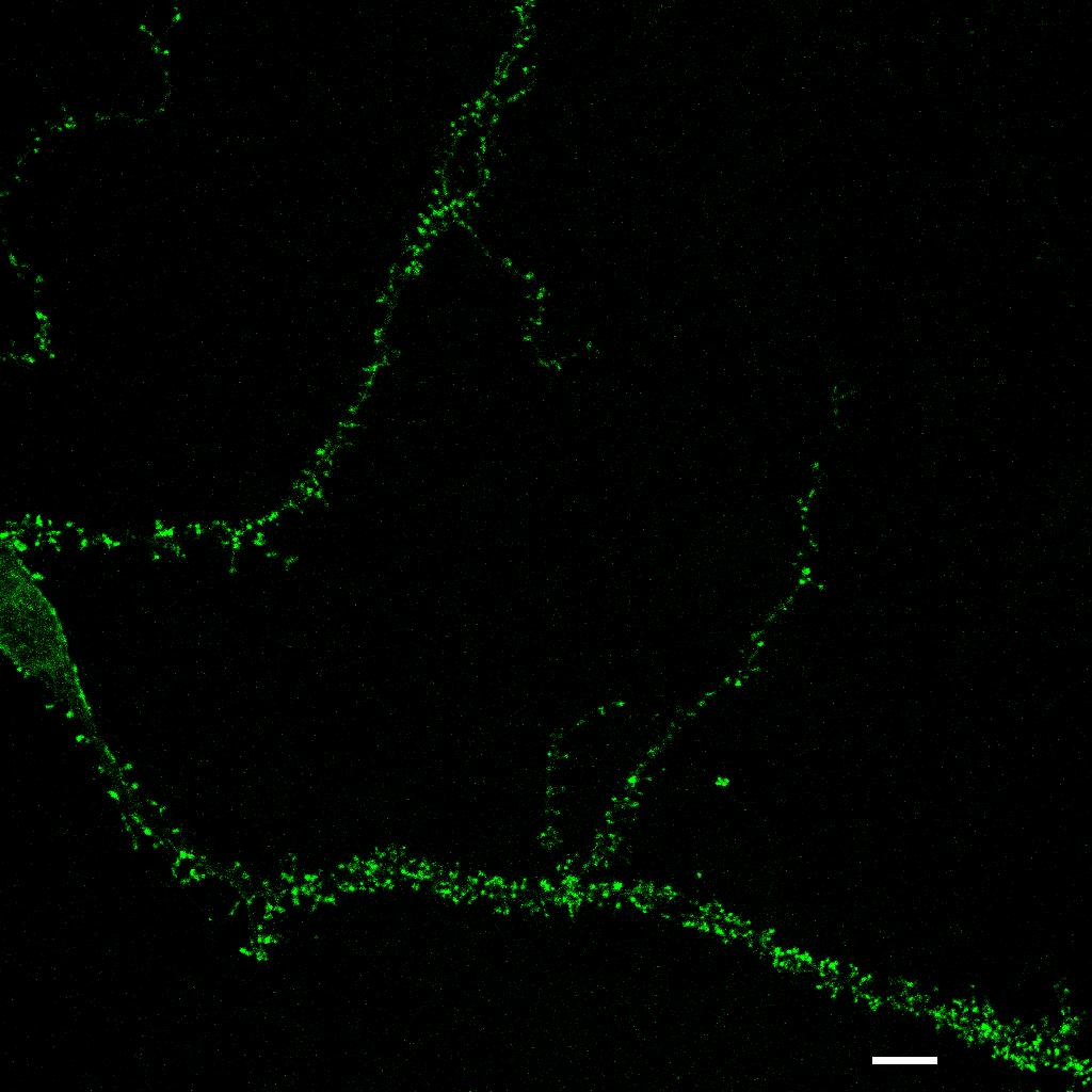
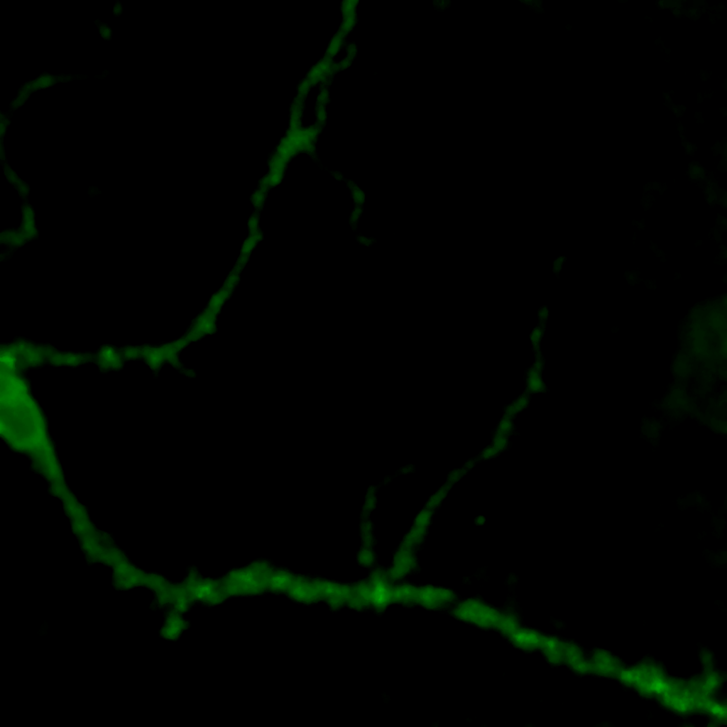
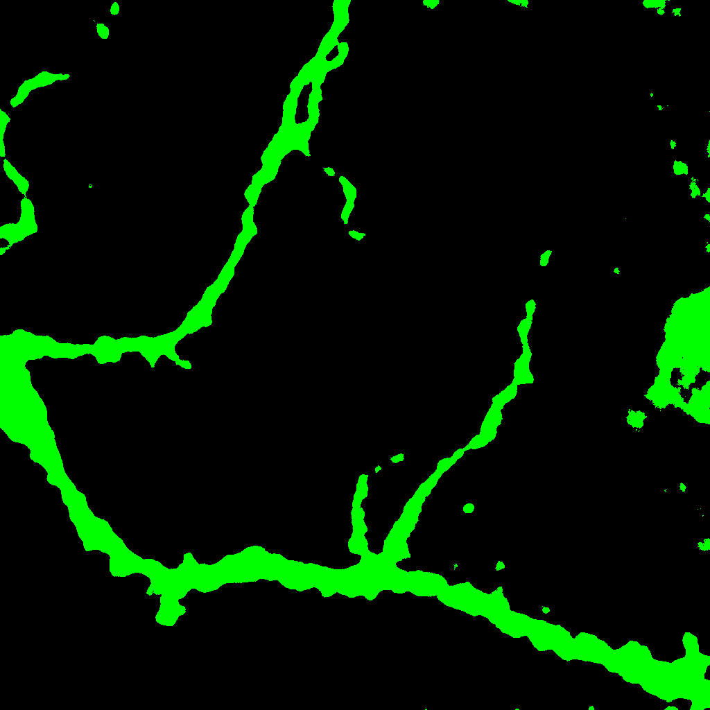
Figure 1: A 21 days in culture rat hippocampal neuron in culture, transfected with Actin-GFP. (a) Maximum intensity projection from a z-stack. (b) Median filter of the same image. (c) Huang’s thresholding method applied to the same image. Scale bar 5 $\mu$M.

Our method to detect the neuronal structure from images, like the one of Figure 1, can be split into two steps, which will be called respectively salt-and-pepper removal and persistent. In the former one, we reduce the salt-and-pepper noise, and in the latter one we dismiss the elements which appear in the image but which are not part of the structure of the main neuron (astrocytes, other neurons and so on).

In order to carry out the task of reducing the salt-and-pepper noise, we apply the following process both to the images of the stack and to the maximum intensity projection image. Firstly, we apply a low-pass filter [5] to the images. In our case, the filter which fits better with our problem is the median one, since such a filter reduces speckle noise while retaining sharp edges. The filter length is set to $10$ pixels for the situation described in Section 2, this value has been pragmatically determined and it is the only parameter of the whole method which must be changed if the acquisition procedure is modified. The result produced for the maximum intensity projection image of Figure 1 is shown in Figure 1.

Afterwards, we obtain binary images using Huang’s method [14]. This procedure automatically determines an adequate threshold value for the images. Applying that method to the image of Figure 1, we obtain the result depicted in Figure 1.

However, in the image of Figure 1 we can see elements which does not belong to the main neuronal structure. Let us explain how we manage to remove those undesirable elements.

It is worth noting that in every slide of a z-stack appears part of the neuronal structure. On the contrary, irrelevant elements just appear in some of the slides. This will be the key idea of our method.

More concretely, we proceed as follows. As we have explained previously, we apply the salt-and-pepper removal step to all the slides of the z-stack, the result of that in our case study can be seen in Figure 2.

Figure 2: Processed median and Huang’s filter of each z-stack plane from Figure 1 neuron.

In the persistent step, we firstly construct a filtration of the binary image associated with the maximum projection image. A monochromatic image, ${\mathcal{D}}$, can be seen as a set of black pixels (which represent the foreground of the image), and a filtration of ${\mathcal{D}}$ is a nested subsequence of images $D^{0}\subseteq D^{1}\subseteq\ldots\subseteq D^{m}=\mathcal{D}$.

In order to construct a filtration of the binary image associated with the maximum projection image we proceed as follows. $D^{m}$ is the maximum projection image. $D^{m-1}$ consists of the connected components of $D^{m}$ whose intersection with the first slide of the stack is non empty. $D^{m-2}$ consists of the connected components of $D^{m-1}$ whose intersection with the second slide of the stack is non empty, and so on. In general, $D^{m-n}$ consists of the connected components of $D^{m-n+1}$ whose intersection with the $n$-th slide of the stack is non empty. In this way, a filtration of the maximum projection image is obtained, see Figure 3.

Figure 3: A series of pictures depicting the process of filtration from the z-stack of Figure 1. From $D^{0}$ to $D^{8}$: Starting on $D^{0}$ and following to $D^{8}$ each level of the filtration represent the containing, $\subseteq$ information from the previous level. $D^{8}$ contains all the connected components from the image.

As we know that the neuron appears in all the slides of the stack, the component $D^{0}$ of our filtration will be the structure of the neuron. As a final remark, we can notice that the construction of the filtration reaches a point where it is stable; that is, a level of the filtration $D^{i}$ of the filtration such that $D^{j}$ is equal to $D^{i}$ for all $0\leq j<i$. An example can be seen in the components $D^{0}$ to $D^{4}$ of Figure 3. This observation will be important in the next subsection.

3.2 Interpretation in terms of persistent homology

The persistent adjective of the second step of the method presented in the previous subsection comes from the nice interpretation which can be given in terms of the persistent homology theory [9], a branch of Algebraic Topology [18]. In a nutshell, persistent homology is a technique which allows one to study the lifetimes of topological attributes. A detailed description of persistent homology can be seen in [9, 28], here we just present the main ideas.

One of the most important notions in Algebraic Topology is the one of homology groups. The homology group in dimension $n$ of an object $X$, denoted by $H_{n}(X)$, is a set which consists of the $n$ dimensional holes of $X$, also called $n$ dimensional homology classes of $X$. To be more concrete, $H_{0}(X)$ measures the number of connected components of $X$, and the homology groups $H_{n}(X)$, with $n>0$, measure higher dimensional connectedness. In the case of $2$ dimensional monochromatic images, the $0$ and $1$ dimensional homology classes are, respectively, the connected components and the holes of the image; there are not homology classes in higher dimensions.

Now, given a $2$ dimensional monochromatic digital image ${\mathcal{D}}$ and a filtration $D^{0}\subseteq D^{1}\subseteq\ldots\subseteq D^{m}=\mathcal{D}$ of ${\mathcal{D}}$, a $n$-homology class $\alpha$ is born at $D^{i}$ if it belongs to the set $H_{n}(D^{i})$ but not to $H_{n}(D^{i-1})$. Furthermore, if $\alpha$ is born at $D^{i}$ it dies entering $D^{j}$, with $i<j$, if it belongs to the set $H_{n}(D^{j-1})$ but not to $H_{n}(D^{j})$. The persistence of $\alpha$ is $j-i$. We may represent the lifetime of a homology class as an interval, and we define a barcode to be the set of resulting intervals of a filtration.

In the case of the filtrations presented in the previous subsection, the outstanding barcode is the one of $0$ dimensional homology classes. It is worth noting that the structure of the neuron lives from the beginning to the end of the filtration while external elements are short-lived.

For example, the barcode associated with the filtration of Figure 3 is the one depicted in Figure 4.

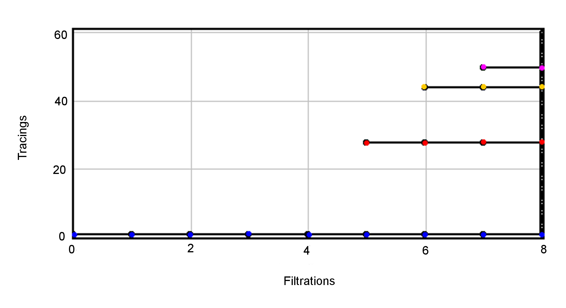
Figure 4: Barcode summary of the filtration process from Figure 3 obtained using NeuronPersistentJ

Let us analyze the information which can be extracted from such barcode. There are several connected components which live is reduced to the maximum projection image, the green connected components of Figure 5, and can be considered as noise. Notwithstanding that the components $x_{1},x_{2}$ and $x_{3}$ (which are respectively the red, yellow and orange connected components of Figure 5) live a bit longer than green components; they are also short-lived; so, they cannot be part of the main structure of the neuron, it is likely that these components come from other biological elements. Eventually, we have the $x_{0}$ component, the blue connected component of Figure 5, which lives from the beginning to the end of the filtration; therefore, as it lives from the beginning to the end of the filtration, it represents the structure of the neuron.

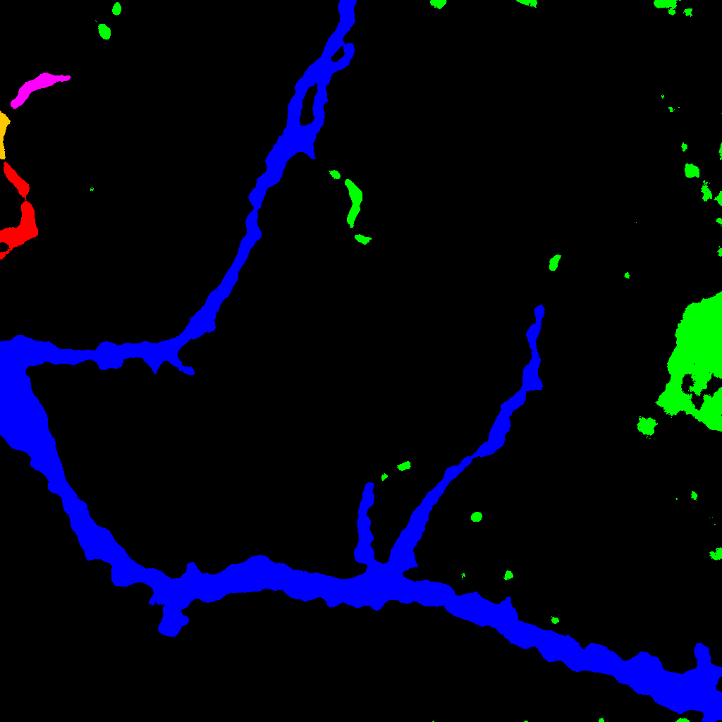
Figure 5: Summary picture of the connected components from Figure 1 projection. Color code: green, components that last one plane. Orange, 2 planes. Yellow, three planes. Red, four planes and blue, components that are present in the eight planes.

We have devised an efficient algorithm to obtain the barcode of $0$ dimensional homology classes associated with the images that we have presented in the previous subsection. This method takes advantage of both the way of building the filtration and the stability of such a filtration. Firstly, we obtain the connected components of the level $0$ of the filtration, $D^{0}$; this is a well-known process called connected component labeling which can be solved using different efficient algorithms, see [21, 16]. Such connected components are $0$ dimensional homology classes which are born at $D^{0}$ and live until the end of the filtration, this fact comes from the filtration construction process. Now, we focus on the level $1$ of the filtration, $D^{1}$. As we have seen at the end of the previous subsection, the filtration has a stability level; therefore, we consider two feasible cases. If $D^{0}$ is equal to $D^{1}$, we can pass to the next level of the filtration. Otherwise, we obtain the connected components which appear at $D^{1}$ but not at $D^{0}$, such components are $0$ dimensional homology classes which are born at $D^{1}$ and live until the end of the filtration. In order to check if $D^{0}$ and $D^{1}$ are equal, we use the MD6 Message-Digest Algorithm [24]. Such algorithm is a cryptographic hash function which given an image returns a unique string; therefore, if the result produced for $D^{0}$ and $D^{1}$ is the same, we can claim that both images are equal. This procedure is faster than comparing pixel by pixel the images.

The above process is iterated for the rest of the levels of the filtration. In general, if we are in the level $i$ of the filtration, there are two cases: if $D^{i-1}=D^{i}$ (this is tested with MD6 algorithm) then pass to level $i+1$; otherwise the connected components which appear in $D^{i}$ but not in $D^{i-1}$ are the $0$ dimensional homology classes which are born at $D^{i}$ and live until the end of the filtration. In this way, we can obtain the barcode of $0$ dimensional homology classes without explicitly computing persistent homology.

4 Experimental results

The procedure to detect neural structure presented in the previous section has been implemented as a new plugin for ImageJ [23] called NeuronPersistentJ [17]. Figure 6 illustrates the results which are obtained with NeuronPersistentJ using three different examples considering $10$ as the length of the median filter. As can be seen in such examples both the noise and structures of neighbor neurons are removed from the final result.

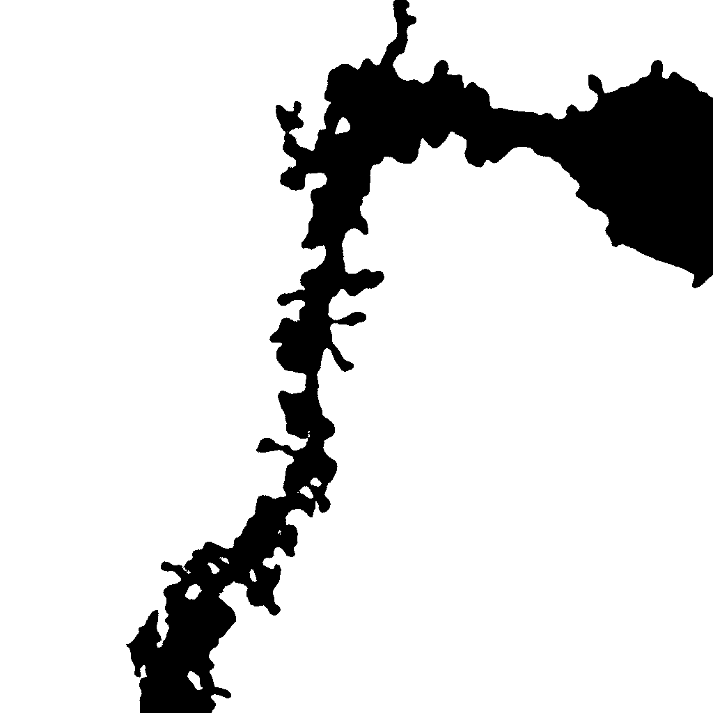
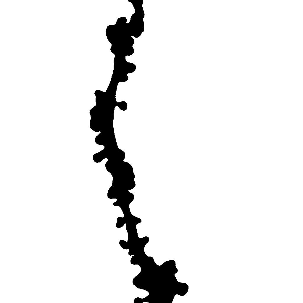
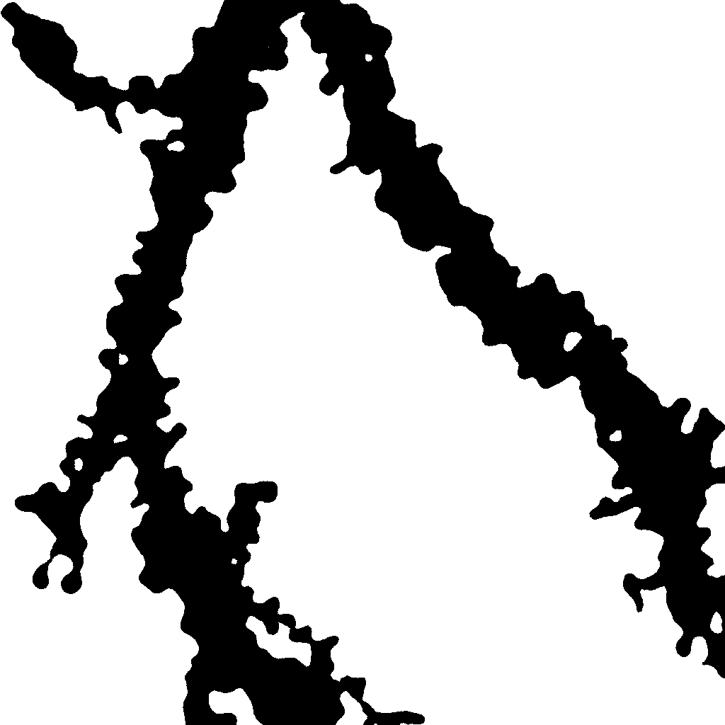
Figure 6: Top (from a to c): Three examples of dendritic fragments of hippocampal neurons in culture transfected with Actin-GFP. Bottom (from a’ to c’): Structures obtained with the NeuronpersistentJ application with a median filter 10.

We have validated our method and plugin with a set of image stacks of real 3D neuron dendrites acquire using the procedure explained in Section 2. In order to test the suitability of our software, we have compared a manual selection of the region of interest with the results obtained using NeuronPersistentJ. The manual selection was performed using the polygonal selection tool from ImageJ. In order to compare the two tracings (the manual and the one obtained using NeuronPersistentJ), we have considered both the accuracy and the efficiency.

The accuracy of the plugin is measured with the three following relevant features: $(1)$ the number of branches obtained with the manual tracing compared with the number of branches detected with NeuronPersistentJ, $(2)$ the area of the region selected manually recognized with NeuronPersistentJ (that is, the intersection, $\cap$, of the region selected manually and the one obtained with NeuronPersistentJ) and $(3)$ the area of the region detected by NeuronPersistentJ which does not appear in the manual tracing with respect to the area which does not contain the manual tracing (i.e. the area of the region recognized by NeuronPersistentJ minus, $\setminus$, the region manually selected with respect to the complement, $\_^{C}$, of the region manually selected). To compute the percentages associated with these features, we use the following formulas.

$$(1) = \frac{\texttt{Number of branches of NeuronPersistentJ tracing}}{\texttt{Number of branches of manual tracing}}\times 100$$

$$(2) = \frac{\texttt{Area (NeuronPersistentJ tracing}\cap\texttt{Manual tracing)}}{\texttt{Area (Manual tracing)}}\times 100$$

$$(3) = \frac{\texttt{Area (NeuronPersistentJ tracing}\setminus\texttt{Manual tracing)}}{\texttt{Area((Manual tracing)}^{C})}\times 100$$

It is worth noting that the higher the values for both $(1)$ and $(2)$ the better since this means that we are close to detect all the branches and the whole region of interest. On the contrary, the value of $(3)$ should be small in order to avoid the inclusion of regions which are not relevant.

The experimental results that we have obtained with our dataset, considering different lengths for the median filter, using NeuronPersistentJ are shown in Table 1. As we are seeking an equilibrium between the values of the features $(2)$ and $(3)$, the best value for the length of the filter is $10$.

	$(1)$	$(2)$	$(3)$
5	$96.2\%$	$78.06\%$	$4.43\%$
10	$98.2\%$	$93.3\%$	$4.19\%$
15	$98.7\%$	$94.9\%$	$6.25\%$

Table 1: Percentages of accuracy of NeuronPersistentJ. $(1)$ Percentage of components detects with NeuronPersistentJ versus manual tracking. $(2)$ Percentage of area detected with NeuronPersistentJ versus manual tracking. $(3)$ Percentage of area draw by NeuronPersintentJ not present in the manual tracking. Percentage is the mean value from eight images.

Let us consider the efficiency of the plugin. As we have explained previously the manual method to select the region of interest consists in using the polygonal tool of ImageJ in the maximum projection image. This manual procedure takes approximately three minutes per neuron. On the contrary, the results are obtained in half the time using NeuronPersistentJ. This is quite relevant since in order to test the effect of some experimental treatments over neurons we do not study just one neuron but batteries of neurons. Therefore, the use of NeuronPersistentJ means a decreasing of the time invested to detect the neuronal structure.

In view of the results, our method can be considered as a good approach, both from the accuracy and efficiency point of view, to automatically trace neuronal morphology from z-stacks.

5 Discussion

The geometric persistence method reported here has been used to develop an ImageJ/Fiji plugin able to extract the neuronal structure. In particular, the contour of the neuron is segmented and therefore the region of interest is recognized.

The application is based on the fact that the neuron structure is present, “or persists”, in all the levels of z-stack images. Our plugin, automatically, generates a digital 2D representation of a three-dimensional neuron in the final picture. After the extraction process, structures from neighbor neurons, background noise and unspecific staining are eliminated from the final image.

The plugin works analyzing every optical plane and comparing the maximum intensity projection with the slides of the z-stack. After a preprocessing step where the salt-and-paper noise is removed, using the median filter, from the slides of the z-stack and the maximum intensity projection, the plugin removes from the maximum intensity projection the elements which does not live enough (i.e. the elements which do not appear in all the slices of the stack) obtaining as result the structure of the neuron.

Histological and imaging protocols are crucial to determine the number of neurons that would be stained and their relative signal to the background of the images. In this report we have chosen the transfection of a GFP protein (Actin-GFP) in hippocampal neurons in culture. Electroporation after plating renders a large number of transfected cells 48 hours after electroporation [20]. During the successive days in culture neuronal density of transfected cells decay slowly to a final density of $20-30$ neurons in a $12$ mm coverlips. Therefore, this culture conditions allows the growing of fully develop neurons withing a broad distance from another transfected neuron. The high GFP quantal yield, results in a excellent contrast staining, improving signal/background ratio. Moreover the plasmid vector employed a PDGF-neuronal promoter, ensuring physiologic levels of expression; as it was previously reported cells could undergo Actin-GFP expression without further developmental problems [20].

To validate our method we have compared a manual surface tracking employing the polygonal selection from ImageJ. The validation uses as a control the total area delimiting by a manual tracing and compares it with the area delimited by NeuronPersistentJ. It is worth noting that the result of the comparison depends on the value of the length of the low pass filter selected; large values will led to a broad structure, on the contrary small values will produce sharp and more defined images. Employing this validation method our results indicate that NeuronPersistentJ is suitable to carry out the recognition of the neuron structure.

The number of manipulations during the reconstruction process is always a drawback for a fully automatic process. NeuronPersitentJ requires a set of binary images; thus, selection of the length of a low-pass filter value that retains the maximal information from the z-stack pictures is the only parameter determined by the experimenter and clearly it depends on the images conditions. NeuronPersitentJ, as other public or commercial available plugins, works better with highly contrasted images, such the ones obtained by inmunofluorescence. The topological approach employed here and the use of binary pictures is independent from the nature of the picture. However, as mentioned, highly contrasted pictures and a clear and continuous staining are key elements for a fine reconstruction.

Skeletonization of neuronal structure has been a popular solution to neuronal reconstruction and structure extraction [19]. Most of the public and commercial solutions available require a manual or semi manual process. Drawing the structure, connecting the dendritic fragments or selecting end or branching points are typical approximations. NeuronPersitentJ renders an automatically structure into a 2D image that contains only the connected dendrites of the neuron. The image can easily been implemented to an automatic Sholl analysis to quantify changes in dendritic morphology. Even though, our plugin must be consider as a first step in the full process of reconstruction.

As mentioned, NeuronPersistentJ would be used a basic towards the automatic detection and clasification of diferent features of neuronal structure, such spine density or dendritic arborization.

Information Sharing Statement

NeuronPersistentJ is available through the ImageJ wiki (http://imagejdocu.tudor.lu/) using the link http://imagejdocu.tudor.lu/doku.php?id=plugin:utilities:neuronpersistentj:start. NeuronPersistentJ is open source; it can be redistributed and/or modified under the terms of the GNU General public License.

References

- [1] Ballesteros-Yáñez, I., et al.: Density and morphology of dendritic spines in mouse neocortex. Neuroscience 138(2), 403–409 (2006)
- [2] Bankder, G., Goslin, K.: Culturing nerve cells. Cellular and Molecular Neuroscience Series. The MIT Press (1998)
- [3] Cajal, S.R.: Conexión general de los elementos nerviosos. La Medicina Práctica 2, 341–346 (1889)
- [4] Calderón de Anda, F., et al.: Autism spectrum disorder susceptibility gene TAOK2 affects basal dendrite formation in the neocortex. Natural Neuroscience 15(7), 1022–1031 (2012)
- [5] Castleman, K.: Digital Image Processing. Prentice-Hall (1996)
- [6] Colicos, M.A., Collins, B.E., Sailor, M., Goda, Y.: Remodeling of Synaptic Actin Induced by Photoconductive Stimulation. Cell 107(5), 605–616 (2001)
- [7] Cuesto, G., et al.: Phosphoinositide-3-Kinase Activation Controls Synaptogenesis and Spinogenesis in Hippocampal Neurons. The Journal of Neuroscience 31(8), 2721–2733 (2011)
- [8] Donohue, D.E., Ascoli, G.A.: Automated reconstruction of neuronal morphology: an overview. Brain Research Reviews 67(1–2), 94–102 (2011)
- [9] Edelsbrunner, H., Letscher, D., Zomorodian, A.: Topological persistence and simplification. Discrete Computional Geometry 28, 511–533 (2002)
- [10] Elston, G.N., DeFelipe, J.: Spine distribution in cortical pyramidal cells: a common organizational principle across species. Progress in Brain Research 136, 109–133 (2002)
- [11] Goedert, M., Spillantini, M.G.: A Century of Alzheimer’s Disease. Science 314, 777 (2006)
- [12] Govindarajan, A., et al.: The dendritic branch is the preferred integrative unit for protein synthesis-dependent LTP. Neuron 69(1), 132–146 (2011)
- [13] Heck, N., et al.: A deconvolution method to improve automated 3D-analysis of dendritic spines: application to a mouse model of Huntington’s disease. Brain Structure and Function 217(2), 421–434 (2012)
- [14] Huang, L.K., Wang, M.J.J.: Image thresholding by minimizing the measure of fuzziness. Pattern Recognition 28(1), 41–51 (1995)
- [15] Landmesser, L.: Axonal outgrowth and pathfinding. Progress in Brain Research 103, 67–73 (1994)
- [16] Lee, D.R., et al.: FPGA based connected component labeling. In: Proceedings International Conference on Control, Automation and System, pp. 2313–2317 (2007)
- [17] Mata, G.: NeuronPersistentJ. Centro Investigación Biomédica de La Rioja - University of La Rioja (2012). http://imagejdocu.tudor.lu/doku.php?id=plugin:utilities:neuronpersisten%tj:start
- [18] Maunder, C.: Algebraic Topology. Dover (1996)
- [19] Meijering, E.: Neuron tracing in perspective. Cytometry Part A 77(7), 693–704 (2010)
- [20] Morales, M., Colicos, M.A., Goda, Y.: Actin-dependent regulation of neurotransmitter release at central synapses. Neuron 27(3), 539–550 (2000)
- [21] Rakhmadi, A., et al.: Connected Component Labeling Using Components Neighbors-Scan Labeling Approach. Journal of Computer Science 6(10), 1096–1104 (2010)
- [22] Ramón-Moliner, E.: The Golgi-Cox technique. Contemporary Methods in Neuroanatomy pp. 32–55 (1970)
- [23] Rasband, W.S.: ImageJ: Image Processing and Analysis in Java (2003). http://rsb.info.nih.gov/ij/
- [24] Rivest, R.L., et al.: The MD6 hash function A proposal to NIST for SHA-3. Tech. rep. (2008)
- [25] Schindelin, J., et al.: Fiji: an open-source platform for biological-image analysis. Nature Methods 9(7), 676–682 (2012)
- [26] Tessier-Lavigne, M., Goodman, C.S.: The molecular biology of axon guidance. Science 274(5290), 1123–1133 (1996)
- [27] Velez-Pardo, C., et al.: CA1 hippocampal neuronal loss in familial Alzheimer’s disease presenilin-1 E280A mutation is related to epilepsy. Epilepsia 45(7), 751–756 (2004)
- [28] Zomorodian, A.: Computing and comprehending topology: Persistence and hierarchical morse complexes. Ph.D. thesis, University of Illionois at Urbana-Champaign (2001)